


1. Introduction
Rolls and streaks, and their role in instability dynamics and laminar–turbulent transition, have been extensively studied in the context of wall-bounded shear flows (Butler & Farrell Reference Butler and Farrell1992; Jiménez Reference Jiménez2013). Rolls, defined as vortices in the cross-plane of the flow, transport high-speed fluid towards the wall and low-speed fluid away from the wall, thereby creating streaks in the main flow velocity (‘lift-up effect’; Landahl Reference Landahl1975). These streaks are themselves subject to instabilities (Park, Hwang & Cossu Reference Park, Hwang and Cossu2011), and are even assumed to play a central role in the self-sustained process of wall-bounded turbulence (Waleffe Reference Waleffe1997; Hwang & Cossu Reference Hwang and Cossu2010). However, the very presence of rolls and streaks in free shear flows such as jets has seldom been recognised until recently. Nogueira et al. (Reference Nogueira, Cavalieri, Jordan and Jaunet2019) documented the appearance of streaky structures in the turbulent velocity field of a high-speed jet, by processing particle image velocimetry data with spectral proper orthogonal decomposition. A linear analysis of the mean flow confirmed that the transient growth of these structures is caused by the lift-up effect. Pickering et al. (Reference Pickering, Rigas, Nogueira, Cavalieri, Schmidt and Colonius2020) investigated the formation of streaks in developing jets, obtained from large-eddy simulation, in response to harmonic forcing input, concluding that streaks may be expected to dominate perturbations in jets at low frequencies.
A linear analysis of the growth of streaks in round jets was conducted by Jiménez-González & Brancher (Reference Jiménez-González and Brancher2017), who computed optimal initial conditions for transient energy growth. These were found to take the shape of rolls, leading to the creation of streaks. Marant & Cossu (Reference Marant and Cossu2018) performed similar transient growth calculations for a parallel plane shear layer. Those authors then went on to characterise the influence of finite-amplitude streaks on the linear Kelvin–Helmholtz instability. It was found that ‘sinuous’ streak structures have a stabilising effect, whereas ‘varicose’ structures destabilise the Kelvin–Helmholtz eigenmode over certain parameter regimes. A similar analysis of wake flows was conducted by Del Guercio, Cossu & Pujals (Reference Del Guercio, Cossu and Pujals2014), where the situation was found to be different: both the sinuous and varicose structures reduce the maximal growth rate, and the varicose streaks have a more stabilising effect than sinuous streaks of the same amplitude. A quadratic variation of the eigenvalues with respect to the streak amplitude was found in both of these works, consistent with results from a second-order sensitivity analysis.
On the basis of these recent studies, the present article investigates how the presence of rolls and streaks modifies the linear instability characteristics of round jets. The scope and study programme are quite similar to the plane shear-layer investigation of Marant & Cossu (Reference Marant and Cossu2018). As streaks in turbulent jets are well modelled using a transient growth analysis (Nogueira et al. Reference Nogueira, Cavalieri, Jordan and Jaunet2019), we evaluate here how optimal rolls and streaks, obtained with a similar procedure, affect the Kelvin-Helmholtz mechanism in jets, which is relevant for understanding the interplay between streaks and the well-documented wavepackets in jets (Jordan & Colonius Reference Jordan and Colonius2013; Cavalieri, Jordan & Lesshafft Reference Cavalieri, Jordan and Lesshafft2019). Differently from (Marant & Cossu Reference Marant and Cossu2018), the curvature of a jet shear layer induces self-interaction effects, and in particular ‘jet-column’ dynamics, which scale with the jet diameter and are absent in single plane shear layers. Jet-column dynamics are similar to the interaction dynamics between the two shear layers that form a plane jet or wake; the absolute mode in round jets without counterflow is of the jet-column type (Lesshafft & Huerre Reference Lesshafft and Huerre2007). While our present study considers only streamwise-invariant base flow settings, the role of streaks in jets is not limited to these. For instance, streak structures have been observed to appear prominently in the braid regions between convecting ring vortices, as shown most recently in the experiments of Kantharaju et al. (Reference Kantharaju, Courtier, Leclaire and Jacquin2020) and in the optimal perturbation analysis of Nastro, Fontane & Joly (Reference Nastro, Fontane and Joly2020).
The paper is organised as follows. In § 2, linearly optimal roll structures are computed, consistent with Jiménez-González & Brancher (Reference Jiménez-González and Brancher2017), that maximise the transient temporal growth of streaks in an axisymmetric jet base flow. The nonlinear flow development, in the presence of finite-amplitude rolls, is then simulated in time. In § 3, frozen instances of streaky parallel jets, obtained in this way, are taken as base flows for linear stability analysis, and the sensitivity of temporal eigenmodes with respect to rolls and streaks is discussed. The maximum temporal mode as well as the absolute growth rate in jets distorted by rolls and streaks are investigated. Conclusions and perspectives are given in § 4.
2. Evolution of rolls and streaks in a parallel jet
We seek roll structures that lead to the fastest growth of streaks in a parallel and initially axisymmetric jet (Jiménez-González & Brancher Reference Jiménez-González and Brancher2017). The initial velocity in the streamwise  $z$ direction is given by the usual profile of Michalke (Reference Michalke1971):
 \begin{equation} W(r)=\frac{1}{2} +\frac{1}{2}\tanh \left[ \frac{1}{4b} \left (\frac{1}{r}-r \right ) \right ], \end{equation}
where  $b$ represents the non-dimensional momentum shear-layer thickness and
  $r$ the radial coordinate. The profile, as all quantities in what follows, is scaled with respect to the jet radius
  $R$ and the centreline velocity
  $W_c$. The viscosity
  $\nu$ of an incompressible fluid is characterised by the Reynolds number,
  $Re = W_c R/\nu$. Values
  $Re=10^{4}$ and
  $b=\frac {1}{20}$ are used throughout this study.
We define rolls as a set of counter-rotating vortices in the cross-stream plane, with radial and azimuthal velocity components  $u_r(r,\theta )$ and
  $u_\theta (r,\theta )$, where
  $\theta$ is the azimuthal coordinate. Through convection, the rolls distort the axisymmetric profile (2.1), such that the streamwise velocity changes in time as
  $W(r)+u_z(r,\theta ,t)$. The perturbation
  $u_z$ represents the streaks. As we limit all following instability analysis to streamwise-invariant base flows, rolls and streaks are assumed to be independent of the streamwise coordinate
  $z$.
$z$.
It is to be clarified at this point that the computation of optimal initial conditions for the transient growth of streaks is not the focus of this study, but only a necessary step for the following instability analysis of streaky base flows. The transient growth scenario over short and long time horizons has been amply documented by Jiménez-González & Brancher (Reference Jiménez-González and Brancher2017). Furthermore, in accordance with that work as well as with Marant & Cossu (Reference Marant and Cossu2018) and the connected studies cited in § 1, we deliberately stay within the classical assumption of a streamwise-invariant base flow (including the rolls and streaks), in order to provide a first characterisation of the effect of streaks on the shear instability in round jets. This choice allows us to restrict the number of parameters, and to arrive at general conclusions from local instability analysis. It is hoped that these will be beneficial for the future analysis of non-parallel streaky jet base flows, which will necessitate a three-dimensional global framework, including nozzle conditions and justifications for turbulent mean flow modelling.
2.1. Optimisation in the linear limit
Following the approach of Jiménez-González & Brancher (Reference Jiménez-González and Brancher2017) and Marant & Cossu (Reference Marant and Cossu2018), and references therein, optimal roll shapes for streak generation are sought in the linear limit of small velocities  $(u_r, u_\theta , u_z) \ll 1$. The number of rolls and streaks around the azimuth is prescribed by an azimuthal wavenumber
  $m$, such that the variations of
  $u_r$,
  $u_\theta$ and
  $u_z$ in
  $\theta$ are given by a factor
  $\mathrm {e}^{\mathrm {i}m\theta }$. In the following, we refer to
  $m$ as the ‘streak wavenumber’.
For a given value of  $m$, temporal eigenmodes of the axisymmetric profile (2.1) are computed, under the restriction of
  $z$-invariance (zero axial wavenumber). These computations are performed in polar coordinates, such that only the radial coordinate is discretised via Chebyshev collocation (Lesshafft & Huerre Reference Lesshafft and Huerre2007), and non-oscillatory eigenmodes (in time) are recovered. The full spectrum of these eigenmodes, which satisfy the incompressibility condition of zero velocity divergence, is then used as a non-orthogonal basis for the optimisation of transient perturbation growth.
The optimal rolls and streaks are identified such that their kinetic energy is maximised in a linear framework. For a perturbation  $\boldsymbol {u}(r,m,t)$, the initial perturbation
  $\boldsymbol {u}_0=\boldsymbol {u} (r,m,t=0)$ is sought such that the quotient
 \begin{equation} \sigma^{2}=\frac{\left \| \boldsymbol{u}(T) \right \|^{2}}{\left \| \boldsymbol{u}_0 \right \|^{2}} \end{equation}
is maximised, where  $T$ is a prescribed finite evolution time. The norm is defined as
  $\| \boldsymbol {u} \|^{2}=\int _{0}^{r_{max}} ( |u_r|^{2}+|u_{\theta }|^{2}+|u_z|^{2} )r\,\textrm {d}r$, where
  $r_{max}$ denotes the maximal radial coordinate in the computation domain. An orthogonal set of optimal and suboptimal initial perturbations
  $\boldsymbol {u}_0$ can then be obtained by singular value decomposition (Schmid & Henningson Reference Schmid and Henningson2001). All three components of perturbation velocity are included in the norms in (2.2), which means that the energies of both rolls and streaks are taken into account.
Identical optimal structures as shown by Jiménez-González & Brancher (Reference Jiménez-González and Brancher2017) are recovered, for the same base flow (2.1) and the same gain definition (2.2), characterised by roll structures in the initial condition  $\boldsymbol {u}_0$ (vorticity in the cross-plane), which give rise to streaks in
  $\boldsymbol {u}(T)$ (axial velocity). These structures, obtained over a time horizon
  $T=1$, are presented in figure 1 for
  $m=2$ and
  $m=6$. Note that the shapes of these rolls and streaks are insensitive to the choice of sufficiently short time horizons, so that
  $T=0.1$ or
  $T=10$ give practically identical results for the optimal initial condition. According to Jiménez-González & Brancher (Reference Jiménez-González and Brancher2017), viscous decay of rolls and streaks becomes important at time scales
  $T=O(1000)$, much larger than the turbulent coherence scales in the jet flows that motivate the present study.

Figure 1. Optimal (a,c,e,g) and first suboptimal (b,d,f,h) linear rolls and streaks for streak wavenumbers  $m=2$ (a,b,e,f) and
  $m=6$ (c,d,g,h). (a–d) Streamwise perturbation vorticity (rolls) at
  $t=0$; (e–h) streamwise perturbation velocity (streaks) at
  $t=T=1$. Red colour is positive, blue colour is negative.
While Jiménez-González & Brancher (Reference Jiménez-González and Brancher2017) computed, through direct–adjoint looping, the optimal initial conditions that lead to the highest gain, the present singular value decomposition technique also allows us to recover the following suboptimals. The optimal and first suboptimal initial perturbations for both example values of  $m$ are shown in figure 1; in analogy with the plane shear-layer results of Marant & Cossu (Reference Marant and Cossu2018), we refer to the optimal structures in figure 1(a,c,e,g) as ‘sinuous’, and to the first suboptimal ones in figure 1(b,d,f,h) as ‘varicose’. Subsequent suboptimal structures are characterised by an increasing number of radial oscillations.
2.2. Nonlinear time stepping
In the following simulations, optimal and suboptimal initial conditions ( $u_r, u_\theta$) are projected onto a two-dimensional Cartesian mesh in the (
 $x,y$) cross-plane, and are added with a finite amplitude to the initially axisymmetric streamwise base flow velocity profile (2.1). This perturbed base flow is then advanced in time, according to the complete nonlinear Navier–Stokes equations for incompressible flow,
 \begin{gather} \partial_t \boldsymbol{u}+(\boldsymbol{u}\boldsymbol{\cdot} \boldsymbol{\nabla} )\boldsymbol{u}={-}\boldsymbol{\nabla} p + {Re}^{{-}1} \nabla^{2} \boldsymbol{u}, \end{gather}
 \begin{gather}\boldsymbol{\nabla} \boldsymbol{\cdot} \boldsymbol{u} =0, \end{gather}
expressed in Cartesian velocity components. Finite elements, provided by the FEniCS library (Logg & Wells Reference Logg and Wells2010), are used to discretise these equations in the ( $x,y$) plane, and time stepping is performed by use of the Crank–Nicolson method. The velocity components in these Cartesian calculations are denoted
  $\boldsymbol {u} = (U, V, W)$.
Example results from these simulations, with  $m=6$, are shown in figure 2: the first case (figure 2a–d) develops from a sinuous initial condition;the second case (figure 2e–h) starts from a varicose one. The jet deformation due to the sinuous perturbation is more apparent, and reminiscent of the profile shapes of jets from corrugated nozzles (Lajús et al. Reference Lajús, Sinha, Cavalieri, Deschamps and Colonius2019). While the sinuous rolls mostly lead to azimuthal variations of the radial position of the shear layer, the varicose rolls lead to a thickening and thinning of the shear layer at different azimuthal positions. These effects correspond to the parameters
  $R$ and
  $\varTheta$, respectively, of the velocity profiles in Lajús et al. (Reference Lajús, Sinha, Cavalieri, Deschamps and Colonius2019).

Figure 2. Nonlinear time evolution of  $m=6$ streaks in jets: streamwise velocity. (a–d) Sinuous rolls as initial condition (see figure 1g); (e–h) varicose rolls as initial condition (see figure 1h). Both cases start from initial roll perturbations with amplitude
  $A_r(t=0)=3\,\%$, as defined in (2.5). (a)
  $t=2$,
  $A_s=28\,\%$; (b)
  $t=4$,
  $A_s=49\,\%$; (c)
  $t=6$,
  $A_s=63\,\%$; (d)
  $t=16$,
  $A_s=90\,\%$; (e)
  $t=2$,
  $A_s=7\,\%$; (f)
  $t=4$,
  $A_s=13\,\%$; (g)
  $t=6$,
  $A_s=19\,\%$; (h)
  $t=16$,
  $A_s=35\,\%$.
To quantify the intensity of rolls and streaks, their amplitudes  $A_r$ and
  $A_s$ are defined in the same way as in Marant & Cossu (Reference Marant and Cossu2018) and references therein:
 \begin{equation} A_s(t)=\frac{1}{2\max_{x,y}(W_b)}\left ( \max_{x,y}[W(t)-W(0)]-\min_{x,y}[W(t)-W(0)] \right ) \end{equation}
and
 \begin{equation} A_r(t)=\frac{1}{4 \max_{x,y}(W_b)}\left ( \max_{x,y}[U(t)]+ \max_{x,y}[V(t)]-\min_{x,y}[U(t)]- \min_{x,y}[V(t)] \right ). \end{equation}
 The growth of streak amplitude, caused by sinuous and varicose rolls, is shown in figure 3: these computations are initialised with rolls of amplitude  $1\,\% \leqslant A_r \leqslant 3\,\%$, and the streak wavenumber is again chosen as
  $m=6$. The streak amplitude, which initially is zero, is found to increase approximately linearly in time, and the linear growth rate in the initial stage scales with the roll amplitude. The amplitude growth of varicose streaks is slower. As the rolls experience viscous dissipation, their amplitude
  $A_r(t)$ decreases slowly in time. Note that in our parallel-flow setting, rolls generate streaks, but streaks have no influence on rolls, even in the nonlinear regime. Therefore, the roll amplitude may be set as an initial condition parameter, whereas the streak amplitude is simply a function of time in the base flow evolution. The streak amplitude is then chosen as a parameter instead of evolution time, because it indicates more directly the intensity of the jet deformation. Snapshots of these time-evolving streaky jets, characterised by the values of
  $m$,
$m$,  $A_r$ and
  $A_s$, and by their sinuous or varicose symmetry, are now taken as base flows for the purpose of linear stability analysis.

Figure 3. Time evolution of (a) the streak amplitude  $A_s(t)$ and (b) the roll amplitude
  $A_r(t)$, both normalised by
  $A_{r}(0)$, with sinuous and varicose rolls of
  $m=6$ as initial perturbations of amplitude
  $A_{r}(0)=1\,\%,2\,\%,3\,\%$.
3. Linear stability analysis
Linear stability analysis is carried out in Cartesian coordinates ( $x,y,z$). Velocity perturbations (
 $u_x', u_y', u_z'$) and pressure
  $p'$ are assumed to take the form of normal modes
  $[u_x',u_y',u_z',p'](x,y,t)=[u_x(x,y),u_y(x,y),u_z(x,y),p(x,y)]\exp (-\mathrm {i}\omega t+ \mathrm {i} kz)$. The linear perturbation equations are
 \begin{align} &-\mathrm{i}\omega u_x+U\partial_x u_x+\partial_x U u_x+V \partial_y u_x + \partial_y U u_y +\mathrm{i} k W u_x + \partial_x p \nonumber\\ &\quad - Re^{{-}1}(\partial_{xx}u_x+\partial_{yy}u_x-k^{2}u_x)=0, \end{align}
 \begin{align} &-\mathrm{i}\omega u_y+U\partial_x u_y+\partial_x V u_x+V \partial_y u_y +\partial_y V u_y +\mathrm{i} k W u_y + \partial_y p \nonumber\\ &\quad - Re^{{-}1}(\partial_{xx}u_y+\partial_{yy}u_y-k^{2}u_y)=0, \end{align}
 \begin{align} &-\mathrm{i}\omega u_z+U\partial_x u_z+\partial_x W u_x+V \partial_y u_z + \partial_y W u_y +\mathrm{i} k W u_z + \textrm{i}k p \nonumber\\ &\quad -Re^{{-}1}(\partial_{xx}u_z+\partial_{yy}u_z-k^{2}u_z)=0, \end{align}
 \begin{align} & \partial_x u_x+\partial_y u_y+\mathrm{i} k u_z=0.\end{align}
Finite-element discretisation is applied by use of the FEniCS library on a two-dimensional mesh in the ( $x,y$) plane. Second- and first-order Lagrangian elements are used to discretise perturbation velocity and pressure, respectively. The discretised equations are assembled as an eigenvalue problem
  ${\boldsymbol{\mathsf{A}}}\boldsymbol {q}=\omega {\boldsymbol{\mathsf{B}}}\boldsymbol {q}$, where the eigenvalues
  $\omega$ and the associated eigenvectors
  ${\boldsymbol {q}=(u_x,u_y,u_z,p)}$ for a fixed
  $k$ are computed via the Arnoldi algorithm. Eigenvalue calculations on the two-dimensional (
 $x,y$) mesh have been validated against the one-dimensional polar formulation used in § 2.1, discretised only in
  $r$, for a strictly axisymmetric base flow. For a wavenumber
  $k=5$, the seven most unstable eigenmodes are compared in figure 4(a), and excellent agreement is found between these two different formulations. Grid convergence is then examined to determine the required number of grid points
  $N$ in the (
 $x,y$) plane, to be used for linear stability analysis. Real and imaginary parts of the dominant eigenvalue (
 $n=0, k=5$) are tracked. The eigenvalue obtained with the largest number of points (
 $N = 22\,041$) is taken as reference, and the relative error
  $\epsilon$, as a function of
  $N$, with respect to this reference value is presented in figure 4(b). A number of
  $N = 15\,821$ grid points is deemed satisfactory, giving convergence within five significant digits, and is kept for the following computations. As nomenclature, we define the temporal growth rate as
  $\omega _i=\textrm {Im}[{\omega }]$ and the frequency as
  $\omega _r=\textrm {Re}[{\omega }]$. We denote the azimuthal wavenumber of eigenmodes
  $n$, so as to distinguish it from the streak wavenumber
  $m$, which characterises the azimuthal periodicity of the streaky base flow.

Figure 4. Validation and mesh convergence of the linear stability results computed in the ( $x,y$) plane. Eigenmodes with streamwise wavenumber
  $k=5$ of an axisymmetric base flow (2.1) are shown. (a) Validation against a polar formulation, where only the radial coordinate is discretised: the seven leading eigenmodes (
 $n=0,\ldots ,6$) computed in the (
 $x,y$) plane (
 $\circ$, red) and in polar coordinates (
 $\times$, blue). (b) Relative error
  $\epsilon$ of the growth rate
  $\omega _i$ (solid line) and the frequency
  $\omega _r$ (dashed line) of the
  $n=0$ eigenmode, as a function of the number of grid points
  $N$ in the (
 $x,y$) plane. Results for
  $N=22\,041$ are taken as reference.
3.1. Linear sensitivity analysis
In the limit of infinitesimal base flow modifications, the effect of streaks on instability eigenvalues (growth rate and frequency) can be predicted by way of sensitivity analysis (Hill Reference Hill1992; Marquet, Sipp & Jacquin Reference Marquet, Sipp and Jacquin2008). In the context of streaks in plane shear layers, Marant & Cossu (Reference Marant and Cossu2018) demonstrated that this analysis needs to be expanded to second order, if one wishes to correctly retrieve the quadratic dependency of eigenmodes on streak amplitude. The same observation had been reported before from studies of instability control in plane two-dimensional flows via spanwise-periodic base flow modifications (Hwang & Choi Reference Hwang and Choi2006; Tammisola et al. Reference Tammisola, Giannetti, Citro and Juniper2014; Boujo, Fani & Gallaire Reference Boujo, Fani and Gallaire2019). If, however, in the present configuration, rolls and streaks in jets cause first-order variations in the instability eigenvalues, then a sensitivity analysis will allow us to identify roll shapes that optimally destabilise linear eigenmodes.
A given base flow variation  $\delta \boldsymbol {Q}=(\delta U_r,\delta U_{\theta },\delta U_z$) induces a variation
  $\delta {\boldsymbol{\mathsf{A}}}$ of the matrix of the linearised Navier–Stokes operator. The resulting first-order variation
  $\delta \omega$ of the eigenvalue associated with a direct eigenvector
  $\boldsymbol {q}$ and an adjoint eigenvector
  $\boldsymbol {q}^{+}$ (appropriately normalised; see Chomaz (Reference Chomaz2005) for details) is given by
 \begin{equation} \delta\omega=\boldsymbol{q}^{+{\boldsymbol{\mathsf{H}}}}\delta {\boldsymbol{\mathsf{A}}} \boldsymbol{q} = \boldsymbol{s}^{\boldsymbol{\mathsf{H}}} {\boldsymbol{\mathsf{M}}} \delta\boldsymbol{Q}. \end{equation}
The superscript  ${\boldsymbol{\mathsf{H}}}$ denotes the transpose conjugate, the matrix
  ${\boldsymbol{\mathsf{M}}}$ contains mesh-dependent quadrature coefficients for a scalar product and
  $\boldsymbol {s}$ is the base flow sensitivity field (nomenclature as in Lesshafft & Marquet (Reference Lesshafft and Marquet2010)). The effect of a given base flow variation
  $\delta \boldsymbol {Q}$ on the eigenvalue is given by its projection onto the sensitivity field; consequently, if we restrict the norm of
  $\delta \boldsymbol {Q}$ to a fixed value, its optimal shape for maximum destabilisation of an eigenmode is given by the imaginary part of the associated
  $\boldsymbol {s}$.
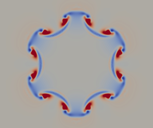
Such a sensitivity field (imaginary part) is shown in figure 5, for an eigenmode with wavenumbers ( $n=3, k=5$) in an axisymmetric (non-streaky) base flow. It can be seen that, at first order, the temporal growth rate is only sensitive to changes in the shear. All components of the sensitivity are found to be axisymmetric, although the underlying eigenmode is not. This result, consistent with the shear layer and wake studies cited above, indicates that rolls and streaks, here defined as non-axisymmetric base flow modifications with zero mean along the azimuth, can only have a second-order effect, but not a first-order effect, on the eigenmodes. Optimisation could be performed on the second-order sensitivity operator to identify azimuthally non-uniform base flow modifications for maximum change of an eigenmode (Boujo, Fani & Gallaire Reference Boujo, Fani and Gallaire2015; Boujo et al. Reference Boujo, Fani and Gallaire2019).

Figure 5. First-order sensitivity of the growth rate with respect to base flow modifications: (a) an instability eigenmode ( $n=3, k=5$) of the axisymmetric base flow (axial velocity); associated sensitivity with respect to (b) radial velocity, (c) azimuthal velocity and (d) streamwise velocity changes in the base flow.
3.2. Linear stability of finite-amplitude streaky jets
Linear stability analysis is now carried out to identify the temporal growth rate  $\omega _i$ of eigenvalues in frozen instances of streaky base flows. For illustrative purposes, the effect of rolls and streaks on the shapes of some eigenmode shapes is shown in figure 6: basic eigenmodes in the axisymmetric case, with azimuthal wavenumbers
  $n=0$, 1 and 2, have been continuously tracked towards high amplitudes
  $A_r$ and
  $A_s$ in base flows with sinuous and with varicose roll and streak structures. In the caption, we extend the use of
  $n$ to the high-amplitude cases in this loose sense of mode tracking, fully aware that the implied symmetries are not strictly preserved in these cases (see the detailed discussion of mode tracking in Lajús et al. (Reference Lajús, Sinha, Cavalieri, Deschamps and Colonius2019)).

Figure 6. Eigenmodes ( $n=0$, 1, 2 and
  $k=5$) of axisymmetric and streaky jets, with streak wavenumber
  $m=6$. Sinuous case:
  $A_r=10\,\%$,
  $A_s=40\,\%$; varicose case:
  $A_r=10\,\%$,
  $A_s=51\,\%$. Streamwise velocity is shown. (a)
  $n=0$, no streaks; (b)
  $n=0$, sinuous streaks; (c)
  $n=0$, varicose streaks; (d)
  $n=1$, no streaks; (e)
  $n=1$, sinuous streaks; (f)
  $n=1$, varicose streaks; (g)
  $n=2$, no streaks; (h)
  $n=2$, sinuous streaks; (i)
  $n=2$, varicose streaks.
Systematic variations of the dominant temporal growth rate ( $n=0$) over streamwise wavenumber
  $k$ are represented in figure 7. Amplitudes
  $A_r=A_s=5\,\%$ are fixed, and instability growth rates are plotted for streak wavenumbers
  $m=1,\ldots ,10$. The range of unstable wavenumbers is narrowed in the presence of sinuous streaks, but largely widened for cases with varicose streaks.

Figure 7. Temporal growth rate  $\omega _i$ as a function of
  $k$ and
  $m$ for
  $A_r=A_s=5\,\%$. Only positive (unstable) values are represented. The first row with label ‘none’ represents the growth rate found for the axisymmetric base flow without streaks. (a) Sinuous rolls/streaks. (b) Varicose rolls/streaks.
In figure 8(a), the maximum  $\omega _i$ over all streamwise wavenumbers
  $k$, denoted as
  $\omega _{i,max}$, is presented as a function of
  $A_s(t)$. The sinuous perturbations, decreasing
  $\omega _{i,max}$, have a stabilising effect, whereas the varicose perturbations, increasing
  $\omega _{i,max}$, destabilise the jets. The maximum temporal growth rate of a streaky jet with sinuous perturbations does not strongly change as the streaks gain amplitude, whereas that with varicose perturbations increases monotonically with the streak amplitude. These results are consistent with the findings of Lajús et al. (Reference Lajús, Sinha, Cavalieri, Deschamps and Colonius2019): the sinuous streaks lead to an azimuthal change of the shear layer position (parameter
  $R$ in Lajús et al. (Reference Lajús, Sinha, Cavalieri, Deschamps and Colonius2019)), which has little effect on jet stability. In contrast, the varicose streaks lead to azimuthal variations of the shear-layer thickness (parameter
  $\varTheta$ in Lajús et al. (Reference Lajús, Sinha, Cavalieri, Deschamps and Colonius2019)), which has a destabilising effect. While it is tempting to discuss these tendencies on the basis of the azimuthally averaged base flow distortions, Marant & Cossu (Reference Marant and Cossu2018) and Lajús et al. (Reference Lajús, Sinha, Cavalieri, Deschamps and Colonius2019) have demonstrated that such a discussion is incomplete, because the periodic variations of the base flow contribute to the change of eigenvalues on the same order as their average.

Figure 8. Parameter studies of the temporal growth rate  $\omega _i$. Blue and red symbols represent sinuous and varicose variations of the base flow, respectively. The temporal growth of the purely axisymmetric jet is shown for comparison (dashed line). Maximum growth rate
  $\omega _{i,max}$ (a) as a function of streak amplitude
  $A_s(t)$ for
  $m=6$ and
  $A_{r}(0)=5\,\%$ (circle),
  $10\,\%$ (square) and (b) as a function of streak number
  $m$ for the most destablising
  $k$ for
  $A_r=5\,\%$ and
  $A_s=5\,\%$. (c) Growth rate
  $\omega _i$ as a function of
  $A_{r}$ for
  $m=6$,
  $k=6$ and
  $A_s=0$. The initially axisymmetric (
 $n=0$) eigenmode is tracked in (c).
The effect of the streak wavenumber  $m$ on
  $\omega _{i,max}$ is presented in figure 8(b) for
  $A_r=A_s=5\,\%$. Over all
  $m$ studied, the varicose perturbations lead to an increase of temporal growth rate, while the sinuous perturbations always decrease the temporal growth rate. The same qualitative behaviour, as demonstrated here only for
  $m=6$, is observed at all values of
  $m$, including the special case
  $m=1$ (‘shift-up’ as opposed to ‘lift-up’; see Jiménez-González & Brancher (Reference Jiménez-González and Brancher2017)). In figure 8(c), the changes of the temporal growth rate of the dominant
  $n=0$ eigenmode as a function of small roll amplitude are tracked. It is found that the growth rate variations are initially quadratic in
  $A_r$, which indicates a second-order sensitivity. This is consistent with our findings in § 3.1 that the first-order sensitivity of azimuthally periodic base flow modifications, rolls and streaks, is zero. A quantitative second-order sensitivity analysis is not attempted here, as the result can be expected to be similar to that of Marant & Cossu (Reference Marant and Cossu2018).
3.3. Absolute instability of streaky jets
Although the results of our jet study so far display the same trends as revealed by Marant & Cossu (Reference Marant and Cossu2018) for plane shear layers, the effect of streaks on the absolute instability mode in jets deserves to be examined. In jets, the absolute mode is of the jet-column type (Lesshafft & Huerre Reference Lesshafft and Huerre2007), and therefore physically distinct from the plane shear layer case. In a similar study of parallel wakes, Del Guercio et al. (Reference Del Guercio, Cossu and Pujals2014) observed that sinuous as well as varicose spanwise perturbations may reduce the absolute growth rate and even suppress the absolute instability. Brandt et al. (Reference Brandt, Cossu, Chomaz, Huerre and Henningson2003) demonstrated a similar stabilising effect of streaks on the absolute mode in a Blasius boundary layer.
For our standard jet base flow, variations of the absolute growth rate  $\omega _{0,i}$ (see Huerre & Monkewitz Reference Huerre and Monkewitz1990) with roll amplitude
  $A_r$ are shown in figure 9. The streak amplitude is set to zero in this example. In the case of varicose perturbations, increasing
  $A_r$ slightly increases the absolute growth rate
  $\omega _{0,i}$ for streak wavenumbers
  $m<6$, but even a very high roll amplitude does not give rise to absolute instability. Varicose rolls with
  $m \geqslant 6$ are seen to decrease
  $\omega _{0,i}$. Sinuous rolls are found to have a stabilising effect on the absolute growth rate, higher
  $m$ being more stabilising. Additional computations, not presented here, show that non-zero values of the streak amplitude
  $A_s$ do not lead to further significant destabilisation of the absolute jet-column mode. In conclusion, a situation where rolls and streaks would give rise to absolute instability in jets could not be identified.

Figure 9. Variations of the absolute growth rate  $\omega _{0,i}$ with roll amplitude
  $A_r$. The streak amplitude
  $A_s$ is zero.
4. Conclusions
The effect of rolls and streaks on the local instability properties of round jets has been investigated in this work for various control parameters. First, optimal sinuous and varicose rolls and streaks, in the sense of maximal energy growth, have been identified for prescribed numbers of streaks along the azimuth. Optimal and suboptimal rolls and streaks take a form similar to the sinuous and varicose perturbations found in plane mixing layers. In both scenarios, streaks grow within the jet shear layer due to the lift-up mechanism. Sinuous roll structures impart wavy displacements of the shear layer, whereas varicose rolls lead to periodic variations of its thickness. Nonlinear simulations show that rolls evolve slowly in time, only subject to viscous decay, while streaks experience linear amplitude growth in their initial stage.
Linear stability analysis has been performed on frozen instances from nonlinearly evolved streaky jet flows. The observed trends are clear and easily summarised: sinuous rolls and streaks, which themselves represent the fastest-growing transient structures, induce a decrease in the growth rate of Kelvin–Helmholtz instability modes. Varicose rolls and streaks, in contrast, lead to increased instability. The first-order sensitivity of Kelvin–Helmholtz eigenmodes in a non-streaky jet has been computed, and found to be strictly axisymmetric, even for non-axisymmetric mode shapes. Therefore, the effect of low-amplitude rolls and streaks, with zero axisymmetric projection, cannot be explained from such an analysis. Consistent with this result, the variations of instability growth rates with roll amplitude have been shown to be nonlinear, presumably quadratic, analogous to the more detailed sensitivity studies of plane shear flows in the recent literature.
Finally, the absolute growth rate of the axisymmetric jet-column mode in streaky jets has been examined. Although varicose rolls do lead to a slight destabilisation of this mode, the instability has been found to remain convective over the investigated parameter space. On this basis, the presence of rolls and streaks in jets, although certain to change the quantitative instability properties, is not expected to lead to self-sustainedp oscillations.
The results from the present investigation lead to the conclusion that the presence of rolls and streaks affects the instability properties of round jets in ways similar to those described by Marant & Cossu (Reference Marant and Cossu2018) for the setting of plane shear layers. The inclusion of roll structures in the base flow, compared to the roll-free settings of Marant & Cossu (Reference Marant and Cossu2018), has been found to have a similarly strong, but not qualitatively different effect as the streaks alone. An important limiting assumption in the present study, which is to be relaxed in future work, lies in the restriction to streamwise-invariant rolls and streaks. Despite this limitation, the significant modification of Kelvin–Helmholtz instability growth rates clearly indicates that roll and streak perturbations in jets must be accounted for in future modelling of jet instability behaviour.
Acknowledgements
This work has received funding from the Clean Sky 2 Joint Undertaking under the European Unions Horizon 2020 research and innovation programme under grant agreement no. 785303. The article reflects only the authors' view; the Joint Undertaking is not responsible for any use that may be made of the information it contains.
Declaration of interests
The authors report no conflict of interest.


