


1. Introduction
The operation of marine propellers results in the generation of intense tip vortices. They are problematic for a number of reasons. In particular, they are locations of cavitation phenomena, due to the local minima of pressure achieved within their core (Zhang et al. Reference Zhang, Zhang, Peng, Wang and Shao2015; Park & Seong Reference Park and Seong2017; Peng et al. Reference Peng, Zhang, Wang, Xu, Song, Cao, Liu, Hong and Yan2019). As a result, they affect the structural integrity of the propeller blades at their onset, and all devices placed downstream, such as rudders. In addition, they are source of vibrations and noise, causing additional fatigue and discomfort, and increasing the environmental impact of marine propulsion (Farcas, Thompson & Merchant Reference Farcas, Thompson and Merchant2016; Vakili, Ölçer & Ballini Reference Vakili, Ölçer and Ballini2020, Reference Vakili, Ölçer and Ballini2021). They are also detrimental to the stealth and tactical capabilities of military vessels.
With the purpose of mitigating the above issues, conventional propellers are designed to reduce the load at the tips of their blades. This way, lower gradients are generated between their pressure and suction sides, reducing the intensity of the tip vortices. However, this solution has a negative impact on the efficiency of propulsion. An alternative solution is represented by the use of winglets at the tips of the blades, similar to those adopted on the wings of airplanes. These devices allow splitting the single tip vortex typically generated by a conventional blade into two vortices. This way, the load at the tips of the blades can be increased, resulting in tip-loaded propellers, achieving higher performance and efficiency, equivalent to lower fuel consumption and pollution coming from marine propulsion.
Unfortunately, we are currently very far from a full understanding of the flow physics of tip-loaded propellers with winglets, which would be useful to optimize these devices. Experiments are expensive and challenging, and can provide important but limited information, usually dealing with visualizations of the dynamics of the tip vortices. For instance, Bertetta et al. (Reference Bertetta, Brizzolara, Canepa, Gaggero and Viviani2012) reported laser doppler velocimetry experiments conducted in a cavitation channel, coupled with computations performed by both potential and Reynolds-averaged Navier–Stokes (RANS) solvers. Their study revealed the generation of a couple of vortices from each blade of a propeller with winglets, produced respectively at the leading edge and at the tip of each winglet. A detailed experimental study in this field is also attributable to Amini et al. (Reference Amini, Reclari, Sano, Iino and Farhat2019). They reported experiments on a simplified elliptical blade, exploring a number of geometries of winglets. They were demonstrated to be effective in delaying the inception of cavitation phenomena, while their effect on the lift to drag ratio was found to be almost negligible.
Potentially, more details may be inferred from computational fluid dynamics, but the simulation of the flow physics is very demanding already for conventional propellers, shedding a single tip vortex from each blade. It is not only the onset of the tip vortices that needs to be resolved. In addition, their downstream evolution, mutual interaction and instability require to be reproduced, which is possible only through expensive, high-fidelity, eddy-resolving methodologies on very fine grids. Of course, this challenge is even reinforced in the case of winglets propellers, due to the increased complexity of the geometry and the need to resolve two smaller tip vortices shed by each blade.
To date, only a few works were able to reproduce the dynamics and downstream development of the tip vortices shed by marine propellers by using eddy-resolving methodologies, as detached-eddy simulation (DES) or large-eddy simulation (LES). For instance, DES computations were conducted by Muscari & Di Mascio (Reference Muscari and Di Mascio2013), Muscari, Di Mascio & Verzicco (Reference Muscari, Di Mascio and Verzicco2013), Guilmineau et al. (Reference Guilmineau, Deng, Leroyer, Queutey, Visonneau and Wackers2015), Gong et al. (Reference Gong, Guo, Zhao, Wu and Song2018), Viitanen et al. (Reference Viitanen, Hynninen, Sipilä and Siikonen2018) and Sun et al. (Reference Sun, Wang, Guo, Zhang, Sun and Liu2020). LES was instead utilized by Balaras, Schroeder & Posa (Reference Balaras, Schroeder and Posa2015), Kumar & Mahesh (Reference Kumar and Mahesh2017), Posa et al. (Reference Posa, Broglia, Felli, Falchi and Balaras2019), Asnaghi, Svennberg & Bensow (Reference Asnaghi, Svennberg and Bensow2020), Liao et al. (Reference Liao, Wang, Yang and He2020), Wang et al. (Reference Wang, Wu, Gong and Yang2021), Zhang, Ding & Liang (Reference Zhang, Ding and Liang2021) and Posa, Broglia & Balaras (Reference Posa, Broglia and Balaras2022b). However, those works focused on conventional propellers, with no winglets at the tips of their blades.
A few computational studies are actually available in the literature on tip-loaded propellers with winglets. However, they are based on the solution of the RANS equations on grids consisting of a few million points (Sánchez-Caja, Sipila & Pylkkanen Reference Sánchez-Caja, Sipilä and Pylkkänen2006; Sánchez-Caja et al. Reference Sánchez-Caja, González-Adalid, Pérez-Sobrino and Saisto2012, Reference Sánchez-Caja, González-Adalid, Pérez-Sobrino and Saisto2014a,Reference Sánchez-Caja, González-Adalid, Pérez-Sobrino and Sipiläb; Haimov, Vicario & Del Corral Reference Haimov, Vicario and Del Corral2011; Brown et al. Reference Brown, Sánchez-Caja, Adalid, Black, Pérez-Sobrino, Duerr, Schroeder and Saisto2014; Shin & Andersen Reference Shin and Andersen2017; Gao et al. Reference Gao, Zhu, Liu and Yan2019; Maeda et al. Reference Maeda, Sano, Iino, Farhat and Amini2021) and are not targeted at analysing the wake dynamics. They typically provide results dealing with global performance, load on the blades and cavitation phenomena in the vicinity of the propeller. RANS is also sometimes utilized to verify the results produced by lower-fidelity methodologies, as in the works by Gaggero, González-Adalid & Pérez-Sobrino (Reference Gaggero, González-Adalid and Pérez-Sobrino2016a,Reference Gaggero, González-Adalid and Pérez-Sobrinob) and Kim & Kinnas (Reference Kim and Kinnas2021), where results from boundary element methods are validated through comparisons against more accurate RANS computations. In the studies above, no discussion was reported on the downstream dynamics of the couple of tip vortices shed by each blade as well as that of the overall wake system. This is consistent with the limitations in terms of both grid resolution and computational technique, negatively affecting the simulation of the wake flow and resulting in the quick diffusion of the wake structures. An exception in this field is the work reported by Zhu & Gao (Reference Zhu and Gao2019). However, they adopted LES on a grid consisting of only 11 million points, similar to those typical of lower-fidelity, RANS computations and not well suited to eddy-resolving simulations.
In the present work, the interest in the dynamics of the tip vortices shed by propellers with winglets is driven by the complex flow physics revealed by visualizations from recent experiments, such as those reported in the work by Brown, Schroeder & Balaras (Reference Brown, Schroeder and Balaras2015): a system of helical vortices was generated, consisting of pairs of tip vortices from each blade, joining at a short distance downstream of the propeller plane. Therefore, LES computations were conducted, dealing with the same tip-loaded propeller with winglets as in Brown et al. (Reference Brown, Schroeder and Balaras2015) and a similar, conventional one without winglets, to compare the dynamics of the tip vortices populating their wakes. In particular, results are compared in terms of intensity of tip vortices and instability of the two wake systems as well as resulting turbulent stresses. The additional effect of the interaction between primary and secondary tip vortices shed by the propeller with winglets is included, performing a detailed vortex core analysis dealing with them as well as with the single vortex arising from their joining process. A similar vortex core analysis is reported on the tip vortices shed by the propeller without winglets. In addition, in this study the analysis is extended to the root vortices shed by both conventional and tip-loaded blades, which are demonstrated to have also a significant impact on the wake signature. LES computations were carried out using an immersed-boundary (IB) technique on a cylindrical grid consisting of 5 billion points, orders of magnitude beyond those typically available in the literature. This LES/IB approach was already validated extensively for the simulation of marine propellers in earlier works (Balaras et al. Reference Balaras, Schroeder and Posa2015; Posa et al. Reference Posa, Broglia, Felli, Falchi and Balaras2019, Reference Posa, Broglia and Balaras2022b), where more conventional design solutions were simulated.
This work is organized as the discussion of the methodology in § 2, the overall set-up of the computations in § 3, the analysis of the results in § 4, and conclusions in § 5. In particular, the results section presents an overview of the dynamics of the tip vortices (§ 4.1), a comparison with references in the literature (§ 4.2), the merging process between the couple of tip vortices shed by each blade with a winglet (§ 4.3), and a comparison between the tip and root vortices from the tip-loaded and conventional propellers (§ 4.4).
2. Methodology
The filtered Navier–Stokes (NS) equations for incompressible flows were resolved in non-dimensional form. The subgrid scales (SGS) were accounted for by using the wall-adaptive local eddy-viscosity (WALE) model by Nicoud & Ducros (Reference Nicoud and Ducros1999). This SGS model was already utilized successfully in a variety of flow problems of practical interest (Posa & Broglia Reference Posa and Broglia2021a; Posa, Broglia & Balaras Reference Posa, Broglia and Balaras2021, Reference Posa, Broglia and Balaras2022a). It computes the eddy-viscosity by means of both the deformation and rotation tensors of the resolved velocity field, and is able to reproduce its correct behaviour in the vicinity of walls without ad hoc corrections or damping functions. It also automatically switches off in regions of laminar flow. The enforcement of the no-slip boundary condition on the surface of bodies was achieved by using an IB methodology. This introduces, within the momentum equation, a forcing term that accounts for the action of the body on the flow. This strategy allows relaxing the requirement for the Eulerian grid discretizing the computational domain to fit the geometry of the bodies immersed within the flow. They are represented by means of Lagrangian grids, ‘immersed’ within the Eulerian grid and discretizing the surface of the bodies. This feature of the IB methodology is especially convenient for handling moving bodies, as in the present case: the Lagrangian grids can move within the Eulerian grid with no need of grid deformation or regeneration, by just updating the forcing terms representing the action of the immersed boundaries within the momentum equation. For more details about the particular IB technique utilized to carry out this study, see the works by Balaras (Reference Balaras2004) and Yang & Balaras (Reference Yang and Balaras2006). Several studies using the same solver, dealing with marine propellers and including extensive validations against experiments, are available in earlier publications (Posa & Broglia Reference Posa and Broglia2021b, Reference Posa and Broglia2022a,Reference Posa and Brogliab). Although it should be acknowledged that the use of an IB technique typically requires grids consisting of a much larger number of points, in comparison with body-fitted methodologies, regular grids result in more efficient numerical schemes, reducing the CPU cost per grid point. So the increase in the computational cost is significant, but it is not proportional to the size of the grid. It is also worth noting that regular grids are also convenient in terms of accuracy of the adopted numerical schemes and their conservation properties, which are especially important in eddy-resolving techniques, such as LES. This advantage is actually reinforced in the case of moving bodies, for which body-fitted methods typically require grid deformation/regeneration and interpolations of the solution between grids, which are also detrimental to efficiency and accuracy.
The NS equations were discretized in space on a staggered cylindrical grid, using second-order central differences. As demonstrated by Fukagata & Kasagi (Reference Fukagata and Kasagi2002), this strategy achieves the exact conservation of mass, momentum and kinetic energy by the discretized version of the NS equations, with beneficial outcomes on the accuracy of the solution. The singularity of the grid at the axis is not a problem for the pressure variable and the azimuthal and axial velocity components. The former is defined at the cell centres, while the azimuthal and axial velocities are defined at the cell faces orthogonal to the azimuthal and axial directions, respectively. Therefore all of them are not defined at the grid axis. Their value there comes instead from interpolations between the first layer of cells in the radial direction and a neighbouring layer of ghost cells. For the radial velocity variable, the problem of the singularity at the axis is avoided by resolving the radial component of the momentum equation for  $q_r=r u_r$, which is by definition equal to zero at the axis. More details on the subject can be found in Verzicco & Orlandi (Reference Verzicco and Orlandi1996). The advancement of the solution in time was conducted using a fraction-step technique (Van Kan Reference Van Kan1986). The discretization in time of all convective, viscous and SGS terms utilized the explicit three-step Runge–Kutta scheme. However, to relax the stability requirements on the time step, the terms of azimuthal derivative in the vicinity of the wake axis were discretized using the implicit Crank–Nicolson scheme. This is also the case for the terms of radial derivative in the vicinity of the tips of the propeller blades, where the grid was refined to resolve properly the onset and downstream evolution of the tip vortices. The hepta-diagonal Poisson problem arising from the enforcement of the continuity requirement was decomposed into a series of penta-diagonal systems of equations across the radial and axial directions by means of trigonometric transformations along the periodic azimuthal direction. Then each penta-diagonal system was inverted using an efficient direct solver (Rossi & Toivanen Reference Rossi and Toivanen1999). More details about the adopted NS solver can be found in Balaras (Reference Balaras2004), Yang & Balaras (Reference Yang and Balaras2006) and Yang, Preidikman & Balaras (Reference Yang, Preidikman and Balaras2008), where it was demonstrated globally second-order accurate in both space and time on canonical flow problems.
3. Set-up
3.1. Flow problem
Two propellers were simulated, shown in figure 1(a,b), dealing with conventional and tip-loaded geometries, respectively. In particular, the latter is equipped with winglets at the tips of its blades. They are the same propellers analysed by means of experiments and RANS computations in the work by Brown et al. (Reference Brown, Sánchez-Caja, Adalid, Black, Pérez-Sobrino, Duerr, Schroeder and Saisto2014). They will be referred to as BASE and TLP cases, respectively. The TLP propeller was developed by the Naval Surface Warfare Center, Carderock Division, of the US Navy. It includes a pressure side winglet at the tip of each blade. The conventional propeller was designed by Bailar Marine Consulting, enforcing the same design requirements as for the TLP geometry, with the purpose of producing a reference for assessing the performance of the tip-loaded design. Both propellers were required to be five-bladed, fixed-pitch and right-handed, to have a  $30^\circ$ projected skew and a ratio between the radii at the hub and at the tips of the blades equal to 0.225. The design requirements included also the ability to produce a minimum value of thrust (1383 kN at full scale in open-water conditions) for a nominal advance coefficient equal to
  $J=0.923$. Note that the advance coefficient is defined as
  $J=V/nD$, where
  $V$ is the advance velocity,
  $n$ is the frequency of the rotation, and
  $D$ is the diameter of the propeller. Both propellers were designed to achieve their peak performance and not to experience pressure and suction side cavitation at the nominal advance coefficient.

Figure 1. Geometries of the (a) BASE and (b) TLP propellers.
In addition to the evident difference between the two propellers in figure 1, due to the winglets in the TLP case, the conventional blades are characterized by a more dramatic reduction of their chord towards outer radii. Moreover, they feature a decreasing pitch from the root to the tip, that is, a decreasing angle relative to the azimuthal direction, while the tip-loaded blades have an almost constant distribution of their pitch. As a result, the load on the propeller blades is decreasing towards outer radii in the BASE case, while the radial distribution of the load is more uniform in the TLP case. It should be noted that Brown et al. (Reference Brown, Sánchez-Caja, Adalid, Black, Pérez-Sobrino, Duerr, Schroeder and Saisto2014) designed the two propellers for comparison purposes. Of course, just changing the conventional design by adding winglets to its blades would make this comparison easier. Meanwhile, this would result in an unrealistic geometry of the winglets propeller. In contrast, the two propellers were designed to meet the same requirements and provide similar performance. This implies changes affecting the entire span of the blades, in order to distribute the overall load in a different way. In conventional propellers, it achieves its peak at about  $70\,\%$ of the radial extent, and undergoes a drop in the vicinity of the tip. In contrast, winglets propellers are designed by prescribing a more uniform spanwise distribution of the circulation. Additional details dealing with the two geometries can be found in the work by Brown et al. (Reference Brown, Sánchez-Caja, Adalid, Black, Pérez-Sobrino, Duerr, Schroeder and Saisto2014).
In the framework of this study, the two propellers were simulated at the design advance coefficient  $J=0.923$. The Reynolds number of a marine propeller is typically computed considering its characteristic length and velocity scales (blade chord and relative velocity of the flow, respectively) at
  $70\,\%R$, where
  $R$ is the radial extent of the propeller. The Reynolds number of the simulation dealing with the TLP case was equal to
 \begin{equation} Re_{TLP} = \frac{c(70\,\%R) \sqrt{V^2 + (0.7 \times 2 {\rm \pi}n \times R)^2} }{\nu} = 432\,000, \end{equation}
where  $c(70\,\%R)$ is the chord of the propeller blades at
  $70\,\%R$, while
  $\nu$ is the kinematic viscosity of the fluid. This Reynolds number is the same as the one adopted in both model-scale experiments and RANS computations by Brown et al. (Reference Brown, Sánchez-Caja, Adalid, Black, Pérez-Sobrino, Duerr, Schroeder and Saisto2014) to verify the performance of the TLP design and assumed in this study as a reference. It should be also noted that the chord length at
  $70\,\%$ of the tip radius for the BASE geometry is about
  $10\,\%$ smaller than for the TLP propeller, resulting in a similar, but slightly smaller Reynolds number. Both propellers were simulated in open-water conditions, again in agreement with Brown et al. (Reference Brown, Sánchez-Caja, Adalid, Black, Pérez-Sobrino, Duerr, Schroeder and Saisto2014), which means that they ingested a uniform flow, operating in isolated conditions. To reproduce the same set-up adopted in the reference experiments and computations, their geometries included a downstream shaft, as illustrated in figure 1, which prevents the generation of a hub vortex in their wake. This choice has no effect on the blade loads, but it is able to influence the wake dynamics, due to the significant signature on it by the hub vortex (Posa et al. Reference Posa, Broglia, Felli, Falchi and Balaras2019, Reference Posa, Broglia and Balaras2022b). In the experiments, although a downstream shaft does not allow investigating the effect by the hub vortex on the wake dynamics, it makes easier the generation of the clean, uniform inflow conditions of the open-water configuration. The use of an upstream shaft, in contrast, requires the presence of a support placed upstream of the propeller, affecting the flow that it ingests.
3.2. Computational grids and boundary conditions
A cylindrical grid consisting of  $1192 \times 2050 \times 2050$ (5 billion) points across the radial, azimuthal and axial directions was adopted. This grid was designed based on earlier studies conducted on the INSEAN E1658 propeller in open-water conditions, operating at similar values of Reynolds number (Posa et al. Reference Posa, Broglia, Felli, Falchi and Balaras2019, Reference Posa, Broglia and Balaras2022b), where a close agreement with reference experiments (Felli & Falchi Reference Felli and Falchi2018) was verified on both parameters of global performance and wake features. Actually, in comparison with the validation study in Posa et al. (Reference Posa, Broglia, Felli, Falchi and Balaras2019), the resolution was improved in the azimuthal direction across the whole extent of the domain, in the streamwise direction in the wake region, and in the radial direction at the tips of the propeller blades. The geometry of tip-loaded propellers with winglets is indeed significantly more complex at outer radial coordinates, in comparison with that of a conventional propeller. Although a grid refinement study was not conducted, due to computational cost considerations, the comparison with the experiments by Brown et al. (Reference Brown, Sánchez-Caja, Adalid, Black, Pérez-Sobrino, Duerr, Schroeder and Saisto2014) in § 4.2 will show a good agreement.
The grid was stretched in the radial and axial directions, with the purpose of clustering nodes in the vicinity of the propeller blades. The radial and streamwise distributions of the grid spacing are reported in figure 2. The axis of the cylindrical grid was placed on the axis of each propeller, which is the origin of the radial coordinates in the cylindrical reference frame. The origin of the streamwise coordinates was placed on the propeller plane. Figure 2(a) shows that the finest radial spacing of the grid is achieved at the tips of the propeller blades ( $r/D=0.5$), while the minimum axial spacing spans the whole region of the propeller blades. The grid was instead characterized by a uniform angular spacing in the azimuthal direction. It is worth noting that this choice also allowed clustering points in the region of interest of the computational domain, thanks to the cylindrical topology of the grid and its decreasing linear azimuthal spacing from outer to inner radii, where the propeller was placed. In the vicinity of the immersed boundaries, the adopted Eulerian grid resulted in a near-wall resolution of about 4 wall-units. It should be noted that this is an average value, since in the present case the immersed boundaries move through the Eulerian grid. Therefore, the grid resolution actually ranges between 0 and 8 wall-units as the Lagrangian grid rotates during the simulations. Nonetheless, the distance of the interface points of the Eulerian grid from the Lagrangian grid, which are the first points off the wall, always stays small enough to make the linear reconstruction of the solution at the interface points accurate across the whole range of distances. The cylindrical grid discretized a computational domain extending
  $2.5D$ upstream of the propeller plane and
  $5.0D$ downstream, and having a radial extent equal to
  $5.0D$. Uniform axial velocity conditions were enforced at the inlet, convective conditions at the outlet, and Neumann conditions at the lateral cylindrical boundary. A schematic of the dimensions of the domain and boundary conditions is provided in figure 3. The radial size of the domain results in a blockage generated by the propeller equal to only
  $1\,\%$. This is well below the
  $10\,\%$ limit prescribed in the literature (Segalini & Inghels Reference Segalini and Inghels2014).

Figure 2. (a) Radial and (b) axial distributions of the grid spacing.

Figure 3. Dimensions of the cylindrical domain and conditions at its boundaries.
The geometries of both BASE and TLP propellers were discretized using surface grids of triangular elements (see figure 4). They were represented by about 158 000 and 172 000 triangles, respectively. It should be noted that in the regions of the blade geometry characterized by low levels of curvature, the two Lagrangian grids in figure 4 have different levels of resolution. Actually, it was verified that the resolution of the Lagrangian grid in those areas has a negligible influence on the solution, but a significant effect on the efficiency of the solver and the resulting computational cost. The present study adopted an Eulerian IB method. In contrast with Lagrangian IB techniques, the accuracy of the solution is driven mostly by the resolution of the Eulerian grid, while the Lagrangian grid is required only to discretize properly the geometry of the body immersed within the flow. More details can be found in Vanella, Posa & Balaras (Reference Vanella, Posa and Balaras2014) and Posa, Vanella & Balaras (Reference Posa, Vanella and Balaras2017). It should be also considered that the geometry of the tip-loaded blades is more uniform across the spanwise direction, in terms of pitch, camber and chord length. Therefore, although the discretization of their tips needs more elements than for conventional blades, fewer triangles are required at inner radial coordinates. For these reasons the blades with winglets were discretized by a smaller number of elements in the areas of low curvature, reducing in this way the already significant computational cost of the simulations. Thanks to the adopted IB methodology, the rotation of the propeller blades was accounted for by just rotating the Lagrangian grids of the bodies within the stationary Eulerian grid discretizing the computational domain. This rotation was prescribed by the selected value of the advance coefficient. Therefore, no tasks of grid deformation/regeneration were required, with beneficial effects on the accuracy and efficiency of the solution.

Figure 4. Details of the Lagrangian grids of the BASE (a,b) and TLP (c,d) propellers looking from upstream (a,c) and downstream (b,d).
3.3. Time resolution and CPU cost of the simulations
Computations were carried out enforcing a constant Courant–Friedrichs–Lewy number equal to 1, based on the stability requirements of the Runge–Kutta scheme. This stability condition resulted in more than 9000 steps per revolution, or less than  $0.04^\circ$ of rotation of the propeller blades per time step. The flow was developed during two flow-through times, to achieve statistically steady conditions. Then statistics were sampled across 10 full revolutions of the propeller blades. It is worth noting that phase-averaged statistics – i.e. statistics synchronized with the rotation of the propeller – were computed at run time considering a cylindrical grid rotating with the propeller. This strategy avoided the need to store a large number of files of the instantaneous solutions of the flow, while increasing substantially the size of the statistical sample, since all time steps during the simulations were included in the sample. It should be acknowledged that phase averaging is affected by the instability of the wake system. Indeed, phase averages include both the fluctuations due to small-scale turbulence and those associated with the oscillations of the major structures populating the wake flow, as the tip and root vortices, away from their average trajectories. The use of phase averaging was preferred to time averaging for the statistical analysis of the flow features, since the latter is affected by the rotation of the propeller and is not suitable to capture the coherence of the wake flow as well as to identify its break-up, due to instability phenomena.
Simulations were conducted in a high-performance computing environment, using a solver with parallel capabilities on 2048 cores of a distributed-memory cluster (Yang & Balaras Reference Yang and Balaras2006). The overall cylindrical grid was decomposed into cylindrical subdomains in the streamwise direction, and communications between subdomains were handled using calls to message-passing interface (MPI) libraries. The overall computational cost of the simulations was equivalent to about 16 million core hours.
4. Results
4.1. Overview of the flow
Visualizations of the major structures shed by the two propellers are provided in figure 5. Both instantaneous and phase-averaged results are shown, in figures 5(a,b) and figures 5(c,d), respectively. It should be noted that the tip vortices generated by the TLP propeller were found more intense than those from the BASE geometry, so different values of the pressure coefficient were considered for extracting the isosurfaces in figure 5. The pressure coefficient is defined as  $c_p=(p-p_\infty )/(0.5 \rho U_\infty ^2)$, where
  $p$ is the local pressure,
  $p_\infty$ is its free-stream value,
  $\rho$ is the density of the fluid, and
  $U_\infty$ is the free-stream velocity, in this case equal to the advance velocity,
  $V$.
$V$.

Figure 5. Instantaneous (a,b) and phase-averaged (c,d) visualizations through isosurfaces of the pressure coefficient from the (a,c) BASE,  $c_p=-0.4$, and (b,d) TLP,
  $c_p=-0.6$, simulations. Colours show the magnitude of vorticity, scaled by
  $U_\infty /D$.
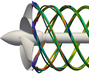
In figure 5, the wake of the BASE propeller displays the typical helical vortices shed from the tips of its blades. The system of tip vortices shed by the propeller with winglets is more complex, consisting in the near wake of a couple of helical structures from each blade. This special feature of the wake is consistent with the visualizations from the experiments reported by Bertetta et al. (Reference Bertetta, Brizzolara, Canepa, Gaggero and Viviani2012) and Brown et al. (Reference Brown, Schroeder and Balaras2015). Details are shown in figure 6, where a lower value of the pressure coefficient is considered. While the BASE propeller generates the typical tip vortex, due to roll-up of vorticity from the pressure side towards the suction side of its blades, the TLP propeller sheds a vortex, indicated as  $\alpha$, from the edge of its winglets, and an additional vortex, indicated as
  $\beta$, produced downstream of the junction between the blades and their winglets. The visualizations in figure 6 also suggest, as discussed more in detail later, that the vortices
  $\alpha$ shed by the TLP propeller are more intense than the tip vortices from the blades of the BASE propeller; the former can be tracked further downstream for the particular value of the pressure coefficient, compared to the latter. However, the tip vortices in figure 6(a) affect a wider area of the surface of the propeller. Although the present simulations do not include a cavitation model, this result suggests that the propeller with winglets is indeed able to limit the intensity of the cavitation phenomena on the surface of the propeller: the region of low pressure on the suction side of the propeller blades extends over a smaller area than for the BASE geometry. This is consistent with the design criteria utilized for the TLP geometry by Brown et al. (Reference Brown, Sánchez-Caja, Adalid, Black, Pérez-Sobrino, Duerr, Schroeder and Saisto2014), targeted at limiting the amount of suction side cavitation. This is also illustrated by means of the contours of figure 7, showing the phase-averaged distribution of the pressure coefficient on the suction side of the propeller blades, looking from upstream. It is evident that the design including winglets is able to maintain higher levels of pressure, relative to the free-stream value, especially at outer radial coordinates, in comparison with the conventional geometry. Meanwhile, it is also able to generate a larger thrust, as discussed later, in § 4.2. This point is also clear in figure 8, dealing with the phase-averaged pressure coefficient on the pressure side of the blades. The highest values are achieved at the tip of the TLP propeller, while for the BASE design, the pressure coefficient undergoes a reduction at the outer radii. In addition, the chord at the tip of the tip-loaded blades is larger than that of the BASE propeller. This also contributes to the generation of higher levels of thrust in the former case.

Figure 6. Phase-averaged visualizations through isosurfaces of the pressure coefficient ( $c_p=-1.6$) from the (a) BASE and (b) TLP simulations. Colours show the magnitude of vorticity, scaled by
  $U_\infty /D$.

Figure 7. Phase-averaged contours of the pressure coefficient over the suction side of the propeller blades from the (a) BASE and (b) TLP simulations.

Figure 8. Phase-averaged contours of the pressure coefficient over the pressure side of the propeller blades from the (a) BASE and (b) TLP simulations.
The vortices  $\alpha$ and
  $\beta$ from the TLP propeller interact with each other and eventually merge into a single helical structure at a short distance downstream, as shown in figure 5. Also, this feature of the wake flow is in agreement with the experiments reported by Bertetta et al. (Reference Bertetta, Brizzolara, Canepa, Gaggero and Viviani2012) and Brown et al. (Reference Brown, Schroeder and Balaras2015). Then these helical vortices remain coherent across a few diameters away from the propeller, in a similar way as for the BASE geometry, as shown in figures 9 and 10 by means of instantaneous and phase-averaged visualizations, respectively. However, both figures 9 and 10 reveal a faster instability of the tip vortices shed by the BASE propeller. In the phase-averaged statistics of figure 10, this result is indicated by the faster diffusion of the signature of the tip vortices in figure 10(a). This difference in the wake development between the BASE and TLP cases and its source will be discussed in more detail in the subsections below. Figure 9 also displays, in the near wake, smaller structures within the wake core, populating the shear layers shed from the trailing edge of the blades. They are more evident in the details of figure 11, especially in the wake of the BASE propeller. They are significantly smaller and not as coherent as the tip vortices, therefore their signature is missing in the phase-averaged visualizations of the wake in figure 10. Figure 11 also highlights that: (i) the single tip vortex resulting from the joining process of the primary and secondary vortices shed by the blades with winglets is larger that that from the conventional ones; (ii) short-wave fluctuations affect the core of the tip vortices already in the near wake; (iii) the root vortices shed by the BASE propeller are much stronger than those from the TLP one.

Figure 9. Instantaneous visualizations through isosurfaces of the pressure coefficient ( $c_p=-0.2$) from the (a) BASE and (b) TLP simulations. Colours show the magnitude of vorticity, scaled by
  $U_\infty /D$.

Figure 10. Phase-averaged visualizations through isosurfaces of the pressure coefficient ( $c_p=-0.2$) from the (a) BASE and (b) TLP simulations. Colours show the magnitude of vorticity, scaled by
  $U_\infty /D$.

Figure 11. Instantaneous visualizations through isosurfaces of the pressure coefficient ( $c_p=-0.4$) from the (a) BASE and (b) TLP simulations. Colours show the magnitude of vorticity, scaled by
  $U_\infty /D$.
Figures 12 and 13 show contours of vorticity magnitude from an instantaneous realization of the solution for the TLP propeller. They highlight the ability of the computational grid to capture the small scales populating the wake. Details are provided in figures 12(b,c) and 13(b,c), where the grid lines are shown respectively at the inner radii of the wake, in the vicinity of the shaft, and at its outer radii, in the vicinity of the tips of the blades.

Figure 12. (a) Instantaneous contours of vorticity magnitude, scaled by  $U_\infty /D$, on a meridian slice of the cylindrical grid in the wake of the TLP propeller. (b) Detail of the grid at the inner radii in the vicinity of the shaft. (c) Detail of the grid at the outer radii in the vicinity of the tip of a blade.

Figure 13. (a) Instantaneous contours of vorticity magnitude, scaled by  $U_\infty /D$, on the cross-section of the cylindrical grid at
  $z/D=0.2$ in the wake of the TLP propeller. (b) Detail of the grid at the inner radii in the vicinity of the shaft. (c) Detail of the grid at the outer radii in the vicinity of the tip of a blade.
4.2. Comparison with the results by Brown et al. (Reference Brown, Sánchez-Caja, Adalid, Black, Pérez-Sobrino, Duerr, Schroeder and Saisto2014)
The work by Brown et al. (Reference Brown, Sánchez-Caja, Adalid, Black, Pérez-Sobrino, Duerr, Schroeder and Saisto2014) provides results on the global parameters of performance for both BASE and TLP propellers, utilized here as a reference. It should be noted that the TLP propeller was actually manufactured and tested experimentally in a towing tank. This is not the case for the BASE propeller, which was instead simulated by RANS.
Table 1 reports a comparison between the results of the present LES/IB computations with those published by Brown et al. (Reference Brown, Sánchez-Caja, Adalid, Black, Pérez-Sobrino, Duerr, Schroeder and Saisto2014) in terms of thrust coefficient, torque coefficient and efficiency. They are defined as
 \begin{equation} K_T = \frac{T }{\rho n^2 D^4},\quad K_Q = \frac{Q}{\rho n^2 D^5}, \quad \eta = \frac{J K_T}{2{\rm \pi} K_Q}, \end{equation}
where  $T$ is the thrust generated by the propeller, and
  $Q$ is the torque acting on its blades.
Table 1. Comparison of the global parameters of performance of the BASE and TLP propellers operating in open-water conditions with the results reported by Brown et al. (Reference Brown, Sánchez-Caja, Adalid, Black, Pérez-Sobrino, Duerr, Schroeder and Saisto2014) for  $J=0.923$.

The results in table 1 display a close agreement between the RANS computations reported by Brown et al. (Reference Brown, Sánchez-Caja, Adalid, Black, Pérez-Sobrino, Duerr, Schroeder and Saisto2014) and the present LES for the BASE propeller, with errors remaining below  $1\,\%$. They are actually larger on the TLP propeller, for which LES/IB provides a slightly higher value of thrust and a lower value of torque in comparison with the experiments by Brown et al. (Reference Brown, Sánchez-Caja, Adalid, Black, Pérez-Sobrino, Duerr, Schroeder and Saisto2014), resulting in a higher efficiency of propulsion. However, the agreement remains quite satisfactory. In addition, it should be noted that the physics shown in § 4.1 is consistent with that discussed by Brown et al. (Reference Brown, Schroeder and Balaras2015) on the same US Navy TLP propeller through both experiments and computations: they revealed the generation of a system of two tip vortices from each blade. Also those vortices were generated at the junction between the blade and the winglet, and at the edge of the winglet, respectively. They were separated initially, but eventually merged at about half a diameter downstream of the propeller. Table 1 also shows how the TLP geometry proposed by Brown et al. (Reference Brown, Sánchez-Caja, Adalid, Black, Pérez-Sobrino, Duerr, Schroeder and Saisto2014) is actually successful in achieving improved performance, compared to the conventional one. This improvement is especially evident in the results from the present simulations.
4.3. Interaction and merging of the tip vortices in the near wake
Figure 5 shows the mutual interaction between the couple of tip vortices shed by each blade with winglet, leading them eventually to merge. For more details, figure 14(a) provides contours of phase-averaged vorticity magnitude at the streamwise coordinate  $z/D=0.2$. The signature of the two tip vortices from each blade is well distinguishable as maxima of vorticity. The tip vortices from the edges of the winglets, characterized by higher values of vorticity, are indicated again as
  $\alpha$, while the ones from the junctions between the blades and the winglets are indicated as
  $\beta$. As the wake develops downstream, the shear between the two tip vortices causes the vortices
  $\alpha$ to rotate around the vortices
  $\beta$, eventually merging with them at about
  $z/D=0.7$ in figure 14( f). Note that the colour scale is shrinking across the panels of figure 14, due to the decreasing streamwise evolution of the maxima of vorticity at the core of the tip vortices.

Figure 14. Contours of phase-averaged vorticity magnitude, scaled by  $U_\infty /D$, downstream of the TLP propeller. Streamwise locations at
  $z/D$ coordinates (a) 0.2, (b) 0.3, (c) 0.4, (d) 0.5, (e) 0.6, ( f) 0.7, (g) 0.8, (h) 0.9, and (i) 1.0. Arrows show the rotational speed of the propeller.
The intense shear between the couple of tip vortices  $\alpha$ and
  $\beta$ is demonstrated in figure 15, where the turbulent shear stress
  $u_r'u_z'$ is shown from phase-averaged statistics. The stress
  $u_r'u_z'$ was computed as a time-averaged product of the fluctuations in time of the radial and streamwise velocity components, relative to their phase averages. Although the behaviour of the other shear stresses was found to be similar, in the region of the interface between the
  $\alpha$ and
  $\beta$ vortices,
  $u_r'u_z'$ achieved the highest values. The highest levels of stress are indeed achieved between
  $\alpha$ and
  $\beta$, which is also consistent with their rotation relative to each other as they develop downstream: note that the vortices
  $\alpha$ gradually move to inner radial coordinates relative to the vortices
  $\beta$. In figure 15, they are identified as local minima of the pressure coefficient, indicated by means of isolines. When the merging process between
  $\alpha$ and
  $\beta$ completes, the levels of shear stresses undergo a substantial decay, confirming that in the near wake, the major source of the stress
  $u_r'u_z'$ is associated with the interaction between
  $\alpha$ and
  $\beta$. Note that the colour scale in figure 15 is again shrinking towards downstream coordinates.

Figure 15. Contours of phase-averaged turbulent shear stress  $u_r'u_z'$, scaled by
  $U_\infty ^2$, downstream of the TLP propeller. Streamwise locations at
  $z/D$ coordinates (a) 0.2, (b) 0.3, (c) 0.4, (d) 0.5, (e) 0.6, ( f) 0.7, (g) 0.8, (h) 0.9, and (i) 1.0. Arrows show the rotational speed of the propeller. White isolines show locations of pressure coefficient
  $c_p=-0.8$.
More details are provided in figure 16, where azimuthal profiles through the cores of the tip vortices are illustrated. Two streamwise locations are considered,  $z/D=0.3$ and
  $z/D=0.7$, corresponding to figures 14(b, f) and 15(b, f). It should be noted that at
  $z/D=0.3$, the tip vortices
  $\alpha$ and
  $\beta$ are still separated, but are roughly aligned along the azimuthal direction, so the same azimuthal profile goes through the core of both tip vortices. At
  $z/D=0.7$, their merging process is already complete. It is also worth noting that figure 16 exploits the symmetry of the phase-averaged statistics, therefore the range of azimuthal coordinates on the horizontal axis goes from
  $0^\circ$ to
  $72^\circ$. In figure 16(a), the position of the core of the two tip vortices is indicated by the minima of the pressure coefficient (dashed lines). At
  $z/D=0.3$, the highest values of shear stress (solid lines) are achieved between them, in the region between
  $62^\circ$ and
  $5^\circ$. At
  $z/D=0.7$, the couple of minima of the pressure coefficient are replaced by a single negative peak, of intermediate magnitude between the minima at
  $z/D=0.3$, coming from the merging of the two vortices
  $\alpha$ and
  $\beta$. The reduction of the shear stresses is dramatic. In figure 16(b), azimuthal profiles for turbulent kinetic energy (solid lines) and vorticity magnitude (dashed lines) are shown. The turbulent kinetic energy was computed as
  $k=0.5 (u_r'u_r' + u_\vartheta 'u_\vartheta ' + u_z'u_z')$, where
  $u_r'u_r'$,
  $u_\vartheta 'u_\vartheta '$ and
  $u_z'u_z'$ are the mean squares of the fluctuations of the radial, azimuthal and streamwise velocity components, relative to their phase averages. As expected, the maxima of turbulence and vorticity correlate with the minima of the pressure coefficient in figure 16(a). At
  $z/D=0.3$, the shear between the vortices
  $\alpha$ and
  $\beta$ results in large levels of turbulent kinetic energy also at azimuthal coordinates between them (see the region around
  $\vartheta =72^\circ$), in addition to the locations of their cores. Again, at
  $z/D=0.7$, the pairs of maxima of both vorticity and turbulent kinetic energy seen upstream are replaced by isolated, weaker peaks associated with a single tip vortex from each propeller blade.

Figure 16. Azimuthal profiles through the core of the tip vortices at the streamwise locations  $z/D=0.3$ and
  $z/D=0.7$ in the wake of the TLP propeller: (a) phase-averaged turbulent shear stress
  $u_r'u_z'$ (solid lines) and pressure coefficient (dashed lines); (b) phase-averaged turbulent kinetic energy (solid lines) and vorticity magnitude (dashed lines). Arrows indicate the azimuthal locations of the cores of the vortices.
4.4. Comparison between the tip and root vortices shed by the two propellers
4.4.1. Intensity of the tip vortices
Contours of phase-averaged azimuthal vorticity are shown in figure 17 in the near wake, providing a comparison between the BASE and TLP cases. They highlight again the presence of two sharp maxima at outer radii just downstream of the TLP geometry, eventually merging into a single vortex. Although also in figure 17(a) a smaller peak of positive vorticity is visible in the near wake in the vicinity of the signature of the tip vortex, it is not actually associated with a secondary tip vortex. As discussed by Kumar & Mahesh (Reference Kumar and Mahesh2017) and Posa et al. (Reference Posa, Broglia, Felli, Falchi and Balaras2019), the propeller wake is characterized by a system of helical vortices across the span of the wake of each blade. They are also distinguishable at inner radii in the wake of the TLP propeller as local minima of azimuthal vorticity. These smaller helical vortices are less intense in comparison with the tip vortices, so their signature is weaker and lost more quickly as the wake develops downstream.

Figure 17. Contours of phase-averaged azimuthal vorticity, scaled by  $U_\infty /D$, on the meridian plane
  $x/D=0$: (a) BASE and (b) TLP cases.
The visualizations in figure 17 point also to significant differences between the two panels across all radii of the propeller wake. These differences will be shown to have an important influence on the downstream development of the tip vortices. Conventional propellers are characterized by a reduction of the load of their blades at outer radii, with the purpose of producing less intense tip vortices. This result is also achieved by decreasing the pitch of the blades, that is, the angle of their profile relative to the azimuthal direction, from the root to the tip. This design results in a wake of each blade having also a decreasing pitch from inner towards outer radii, as shown by figure 17(a), where the wake of each blade stretches across a wide range of streamwise coordinates as it develops downstream. The pitch of the blades of tip-loaded propellers is much more uniform along the radial direction, influencing this way also the wake features, as demonstrated by the contours in figure 17(b): it is larger than for conventional propellers at outer radii, and smaller at inner radii. This feature of the flow results in a delayed shear by the wake of each blade with the tip vortices shed by the preceding blade.
A more detailed comparison is reported in figure 18. In figure 18(a,c,e,g), profiles of vorticity magnitude are shown across the cores of the tip vortices visualized in figure 17. In the label of the horizontal axes of figure 18, the quantity  $l$ refers to the local coordinate centred at the vortex core, while
  $L$ was selected as
  $L=0.05D$. In figure 18, the solid and dashed lines deal with the profiles across the streamwise and radial directions, respectively. At the first location, indicated as
  $\boldsymbol {A}$ in figure 17, the comparison across tip vortices shows that while the vortex
  $\beta$ from the TLP propeller is characterized by a similar intensity as the tip vortex from the BASE propeller, the values of vorticity achieved by the vortex
  $\alpha$ are almost three times higher, indicating that the geometry with winglets fails in producing weaker tip vortices, as a result of the larger level of load at the tip of the propeller blades, in comparison with the BASE design. This is still the case at location
  $\boldsymbol {B}$, where the gap in vorticity values between the two vortices from the TLP propeller declines, as a result of their interaction. Eventually, at location
  $\boldsymbol {C}$, the tip vortices
  $\alpha$ and
  $\beta$ merged into a single structure, characterized by higher levels of vorticity, in comparison with that shed by the BASE propeller. Similar features are still visible at location
  $\boldsymbol {D}$.

Figure 18. Profiles of phase-averaged vorticity magnitude (a,c,e,g) and pressure coefficient (b,d, f,h) through the core of the tip vortices at the locations (a,b)  $\boldsymbol {A}$, (c,d)
  $\boldsymbol {B}$, (e, f)
  $\boldsymbol {C}$, and (g,h)
  $\boldsymbol {D}$ in figure 17. Solid and dashed lines show the profiles through the streamwise and radial directions, respectively. On the horizontal axes, the local coordinate
  $l$ relative to the vortex core is scaled by
  $L=0.05D$.
The differences affecting the intensity of the tip vortices are especially important, since they have an impact on the minima of pressure achieved at their core. They are problematic for the cavitation phenomena that they are potentially able to generate, and the resulting acoustic signature. Therefore, figures 18(b,d, f,h) provide profiles of the pressure coefficient. It is clear that lower levels of pressure are produced at the core of both tip vortices shed by the TLP propeller, in comparison with the single tip vortex shed by the BASE one.
The contours in figure 19 allow us to follow the development of the propeller wake further downstream. They show that the signature of the tip vortices originating from the TLP geometry remains more distinguishable at downstream locations, in comparison with that from the conventional propeller. As noted above and discussed in more detail later, this behaviour is tied not only to the higher intensity of the vortices, but also to their slower process of instability, resulting into a slower diffusion of their signature in the phase-averaged statistics of the flow.

Figure 19. Contours of phase-averaged azimuthal vorticity, scaled by  $U_\infty /D$, on the meridian plane
  $x/D=0$: (a) BASE and (b) TLP cases.
4.4.2. Turbulence at the core of the tip vortices
Contours of phase-averaged turbulent kinetic energy are shown across the near wake in figure 20. Significant differences between figures 20(a) and 20(b) affect not only the tip vortices, extending across all radial coordinates. For instance, the different distribution of the load across the blades results in the generation of intense root vortices at inner radii of the wake of the BASE propeller. They are much weaker downstream of the TLP one. Again, the wake of each blade is much more elongated in the streamwise direction in figure 20(a) than in figure 20(b), as already seen in the vorticity fields. The contours in figure 20 also show that while at their onset the tip vortices shed by the TLP propeller are characterized by higher levels of turbulent kinetic energy, this is no longer the case already at about a diameter downstream. Also in this case, a more detailed comparison between BASE and TLP cases is reported in figure 21, by means of profiles crossing the core of the tip vortices. Again, the solid and dashed lines deal with the profiles along the streamwise and radial directions, respectively.

Figure 20. Contours of phase-averaged turbulent kinetic energy, scaled by  $U_\infty ^2$, on the meridian plane
  $x/D=0$: (a) BASE and (b) TLP cases.

Figure 21. Profiles of phase-averaged turbulent kinetic energy through the core of the tip vortices at the locations (a)  $\boldsymbol {A}$, (b)
  $\boldsymbol {B}$, (c)
  $\boldsymbol {C}$, and (d)
  $\boldsymbol {D}$ in figure 20. Solid and dashed lines show the profiles across the streamwise and radial directions, respectively. On the horizontal axes, the local coordinate
  $l$ relative to the vortex core is scaled by
  $L=0.05D$.
The comparison in figure 21(a), dealing with the location  $\boldsymbol {A}$ in figure 20, is qualitatively similar to that reported above for the vorticity magnitude: the highest levels of turbulent kinetic energy are achieved by far in
  $\alpha$, while
  $\beta$ shows values similar to those within the single tip vortex shed by the BASE propeller. For
  $\boldsymbol {B}$, the values in
  $\alpha$ are closer to those in
  $\beta$, as shown in figure 21(b). Again,
  $\beta$ does not display substantial differences from the tip vortex in the BASE case. Comparisons change for
  $\boldsymbol {C}$. The above discussion, dealing with vorticity maxima and pressure minima, pointed out that the single vortex originating from the merging process between
  $\alpha$ and
  $\beta$ is more intense than the tip vortex from the BASE propeller. Nonetheless, turbulence in figure 21(c) is higher in the latter case. This result is confirmed at the downstream location
  $\boldsymbol {D}$ in figure 21(d). Phase-averaged turbulent kinetic energy is associated with fluctuations relative to statistics synchronized with the rotation of the propeller, due to deviations of the tip vortices from their helical trajectories originating at the tips of the blades. Therefore, the results in figure 21 indicate that in the BASE case, the tip vortices develop a faster instability, leading to their faster break-up, as also shown by the visualizations reported in § 4.1.
The process of faster instability of the tip vortices in the BASE case is illustrated at more downstream locations in figure 22. The outer radii are characterized by a gradual increase of turbulence levels, due to the growing meandering of the tip vortices. This rise is faster for the tip vortices shed by the BASE propeller. Actually, this behaviour affects also inner radial coordinates, although there turbulence is significantly lower. Also figures 22(a) and 22(b) highlight the substantial differences affecting the shear layer shed from the trailing edge of each propeller blade, which will be demonstrated below to be an important source of the faster instability of the tip vortices in the BASE case.

Figure 22. Contours of phase-averaged turbulent kinetic energy, scaled by  $U_\infty ^2$, on the meridian plane
  $x/D=0$: (a) BASE and (b) TLP cases.
Results for the instability of the wake system of both propellers are summarized in figure 23, where the streamwise evolution of the phase-averaged turbulent kinetic energy and shear stresses is reported. At each streamwise coordinate, those quantities were averaged within the fluid domain in the region of radial coordinates  $r/D<0.5$. The highest turbulent stresses are achieved just downstream of the TLP propeller. The initial sharp drop of turbulence levels is followed by a gradual increase, due to the development of instability by the wake system. This is faster downstream of the BASE propeller, as demonstrated by all turbulent stresses. More details are provided in figure 24, where the wake was divided into four regions:
  $0.000 < r/D < 0.125$ (
 ${\boldsymbol {R1}}$),
  $0.125 < r/D < 0.250$ (
 ${\boldsymbol {R2}}$),
  $0.250 < r/D < 0.375$ (
 ${\boldsymbol {R3}}$) and
  $0.375 < r/D < 0.500$ (
 ${\boldsymbol {R4}}$). Averages of the phase-averaged turbulent kinetic energy were computed in each of them. Both BASE and TLP cases show that the growth of turbulence, due to the instability of the wake system, is faster moving from inner to outer radii: it is dominated by the instability of the tip vortices. In contrast, the root vortices, as discussed in detail below, remain more stable and provide a more limited contribution to the downstream rise of the turbulent stresses. The results of figure 24 show also that the streamwise evolution of turbulent kinetic energy in
  ${\boldsymbol {R1}}$ is characterized by a sharp peak at
  $z/D \approx 0.25$. This is due to the separation of the boundary layer on the shaft, because of the contraction of its cross-section.

Figure 23. Streamwise evolution of the phase-averaged turbulent stresses downstream of the BASE and TLP propellers: averages in the region  $r/D<0.5$ for (a)
  $k$, (b)
  $|u_r'u_z'|$, (c)
  $|u_r'u_\vartheta '|$, and (d)
  $|u_\vartheta 'u_z'|$.

Figure 24. Streamwise evolution of the phase-averaged turbulent kinetic energy downstream of the (a) BASE and (b) TLP propellers: averages in the regions  $0.000 < r/D < 0.125$ (
 ${\boldsymbol {R1}}$),
  $0.125 < r/D < 0.250$ (
 ${\boldsymbol {R2}}$),
  $0.250 < r/D < 0.375$ (
 ${\boldsymbol {R3}}$) and
  $0.375 < r/D < 0.500$ (
 ${\boldsymbol {R4}}$).
4.4.3. Root vortices
Figure 19 reveals the signature of additional structures populating the core of the propeller wake. In particular, the vortices shed from the root of the blades are especially intense for the BASE propeller. This is illustrated by means of phase-averaged contours of axial vorticity in figure 25, dealing with cross-stream sections of the propeller wake at increasing downstream distances. At  $z/D=0.5$ (figure 25a), the wake coherence is dominated by the tip and root vortices, which are counter-rotating and co-rotating with the propeller, respectively. The roll-up of the vorticity of the shear layer shed from each blade reinforces the intensity of the root vortices, indicated by
  $\gamma$ and characterized by well-distinguishable maxima of negative vorticity. They remain evident also at downstream coordinates, in contrast with the tip vortices. Although initially the latter have intensity similar to that of the root vortices, they undergo a faster instability, leading to diffusion of the phase-averaged maxima of vorticity, first because of vortex meandering and eventually due to break-up into smaller structures. This is very evident in figure 25( f), dealing with the streamwise coordinate
  $z/D=3.0$.

Figure 25. Contours of phase-averaged streamwise vorticity, scaled by  $U_\infty /D$. Streamwise locations at
  $z/D$ coordinates (a) 0.5, (b) 1.0, (c) 1.5, (d) 2.0, (e) 2.5, and ( f) 3.0, in the wake of the BASE propeller. Arrows show the rotational speed of the propeller.
Figure 26 deals with the wake of the TLP propeller. Significant differences from figure 25 affect not only the tip vortices at the outer radii. This is not surprising, since the design of the TLP propeller is based on a more uniform distribution of the load across the span of the blades, resulting into a reduction at the inner radii and an increase at the outer ones, in comparison with the BASE propeller. In figure 26(a), more, smaller and less intense negative maxima of axial vorticity are visible at inner radii, in contrast with the contours of figure 25(a). In particular, the roll-up of the vorticity populating the wake of the propeller blades into the root vortices, observed in figure 25(a), is missing in the visualization of figure 26(a). Actually, the results at  $z/D=1.0$ in figure 26(b) reveal that the roll-up of the vorticity shed by each propeller blade gives rise to additional structures, at intermediate radii between the tip vortices and the root vortices. In the following, they will be indicated by
  $\delta$, to distinguish them from the root vortices, denoted by
  $\gamma$. The other panels of figure 26 show that also in the wake of the TLP propeller, the downstream decay of the intensity of the maxima of negative vorticity is slower, compared to the positive peaks associated with the tip vortices, because of the slower instability of the vortices at inner radii.

Figure 26. Contours of phase-averaged streamwise vorticity, scaled by  $U_\infty /D$. Streamwise locations at
  $z/D$ coordinates (a) 0.5, (b) 1.0, (c) 1.5, (d) 2.0, (e) 2.5, and ( f) 3.0, in the wake of the TLP propeller. Arrows show the rotational speed of the propeller.
An overview of the differences between BASE and TLP cases is provided through instantaneous isosurfaces of the pressure coefficient in figure 27. Figure 27(a) shows that the root vortices have actually a more significant signature than the tip vortices. The former produce lower values of pressure and are more likely to develop cavitation phenomena and noise. As demonstrated above, the tip vortices in the wake region illustrated in figure 27(a) are still coherent, but they are less intense, so they generate lower pressure minima at their core. Actually, the opposite phenomena occur in the wake of the TLP propeller, since the load across the span of its blades is redistributed towards outer radii. As a result, in the visualization of figure 27(b), using the same value of the pressure coefficient as in figure 27(a), the tip vortices are well captured, while the root ones are not visible, since they are less intense and characterized by weaker pressure minima at their core.

Figure 27. Instantaneous visualizations through isosurfaces of the pressure coefficient ( $c_p=-0.8$) from the (a) BASE and (b) TLP simulations. Colours show the magnitude of vorticity, scaled by
  $U_\infty /D$.
The isosurfaces of the second invariant of the velocity gradient tensor ( $\mathcal {Q}$-criterion; Hunt, Wray & Moin Reference Hunt, Wray and Moin1988) from phase-averaged statistics, visualized in figure 28, are able to isolate the inner helical vortices populating the wake of the propeller. Actually, just downstream of it, the roll-up of the vorticity of the shear layer shed by each blade originates several vortices across the span, but they are not a long-standing feature of the wake flow. An exception is represented by the helical structures, indicated as
  $\delta$, that populate mid-radial coordinates between the root and the tip downstream of the TLP propeller. Therefore, moving away from the propeller plane, while the wake of the BASE propeller is characterized by a system of only two major helical vortices, the tip and root vortices, as shown in figure 28(a), the wake of the TLP propeller is populated by additional inner vortices
  $\delta$, well-distinguishable in figure 28(b), coming from the roll-up of the wake of each blade.

Figure 28. Phase-averaged visualizations through isosurfaces of the second invariant of the velocity gradient tensor ( $\mathcal {Q}D^2/U_\infty ^2=40$) from the (a) BASE and (b) TLP simulations. Colours show the magnitude of vorticity, scaled by
  $U_\infty /D$.
Azimuthal profiles at the radial coordinates of the core of the root vortices are shown in figure 29 for the phase-averaged vorticity magnitude (solid lines) and the pressure coefficient (dashed lines). Exploiting again the symmetry of the configuration, only an angular sector of  $72^\circ$ is considered. Figure 29(a) deals with the streamwise location at
  $z/D=0.5$. It is evident that the root vortices are way more intense in the wake of the BASE propeller, since across its blades the load is shifted towards inner radii. As a result, the peaks of vorticity and negative pressure associated with its root vortices are stronger and sharper than those in the wake of the TLP propeller. At
  $z/D=1.0$ in figure 29(b), the comparison includes also the vortices
  $\delta$ downstream of the TLP propeller, in addition to the vortices
  $\gamma$, which are the root vortices. While the root vortices from the BASE propeller remain much more intense than those from the TLP one, the large structures
  $\delta$ coming from the roll-up of the vorticity in the wake of the tip-loaded blades feature an intensity similar to that for the root vortices
  $\gamma$. This is also the case at the more downstream locations considered in figures 29(c–f), although the fading maxima of vorticity and minima of pressure remain better distinguishable for
  $\delta$ than for
  $\gamma$, since in the latter case the azimuthal profiles are also affected by the boundary layer on the surface of the shaft.

Figure 29. Azimuthal profiles of phase-averaged vorticity magnitude (solid lines) and pressure coefficient (dashed lines) through the core of the vortices  $\gamma$ and
  $\delta$ at the streamwise locations of
  $z/D$ coordinates (a) 0.5, (b) 1.0, (c) 1.5, (d) 2.0, (e) 2.5, and ( f) 3.0. Arrows indicate the azimuthal locations of the cores of the vortices.
The results for turbulent kinetic energy in figure 30 are actually very similar to those in figure 29. Also the maxima of turbulence at the core of the root vortices shed by the BASE propeller are sharper and higher than those in the wake of the TLP propeller. Again, for the latter, the maxima of the azimuthal profiles are mostly hidden by the boundary layer over the shaft, since the root vortices are closer to its surface in comparison with the BASE case. In the wake of the TLP propeller, the levels of turbulent kinetic energy achieved at the core of the vortices  $\delta$ are similar to those at the core of the root vortices
  $\gamma$.

Figure 30. Azimuthal profiles of phase-averaged turbulent kinetic energy (solid lines) and pressure coefficient (dashed lines) through the core of the vortices  $\gamma$ and
  $\delta$ at the streamwise locations of
  $z/D$ coordinates (a) 0.5, (b) 1.0, (c) 1.5, (d) 2.0, (e) 2.5, and ( f) 3.0. Arrows indicate the azimuthal locations of the cores of the vortices.
Overall, the weaker signature of the root vortices in the TLP case, compared to the BASE case, is attributable to the lower load at the root of the TLP propeller. In its wake, the different distribution of the load results in the generation of a couple of major additional vortices within the wake core at intermediate radii between the tip and root vortices, while most of vorticity at inner radial coordinates rolls up into stronger root vortices in the wake of the BASE propeller.
4.4.4. Shear between wake structures
Section 4.4.2 discussed the development of higher levels of phase-averaged turbulent kinetic energy in the near wake of the BASE propeller, due to faster instability phenomena affecting its tip vortices. This behaviour was found tied to the interaction of the tip vortex shed by each blade with the wake from the trailing edge of the following blade. As discussed in earlier works (Posa et al. Reference Posa, Broglia, Felli, Falchi and Balaras2019, Reference Posa, Broglia and Balaras2022b), dealing with the INSEAN E1658 propeller, the tip vortices are characterized by a smaller pitch, compared to the shear layer shed by each blade, which means a slower advancement along the streamwise direction. This feature eventually leads each tip vortex to experience shear with the wake of the following blade at some distance downstream of the propeller, promoting the development of instability, according to the mechanisms of short waves, long waves and mutual inductance discussed in detail by Widnall (Reference Widnall1972) and Felli, Camussi & Di Felice (Reference Felli, Camussi and Di Felice2011). The visualizations above demonstrated that the distribution of the pitch across the spanwise extent of the conventional blades results in more elongated wakes than downstream of the TLP design, leading to their faster interaction with the tip vortices shed by the preceding blades. This is shown by the contours of phase-averaged shear stress  $u_r'u_z'$ in figure 31, whose values at the outer boundary of the propeller wake are higher in the wake of the BASE propeller than downstream of the TLP one, despite the lower intensity of the tip vortices shed by the former. Their signature is identified through minima of the pressure coefficient, indicated again by means of isolines. This signature is better distinguishable in the TLP case, due to the higher intensity of the tip vortices, resulting in stronger minima of pressure at the outer boundary of the propeller wake. The trend observed in the near wake is even reinforced further downstream (figure 32), as the interaction involving the wake structures becomes more complex and their process of instability develops, producing higher levels of shear stress. In addition, the signature of the tip vortices in figure 32 through isolines of
  $c_p$ is lost more quickly downstream of the BASE propeller, because of the faster instability affecting its wake.

Figure 31. Contours of phase-averaged turbulent shear stress  $u_r'u_z'$, scaled by
  $U_\infty ^2$, on the meridian plane
  $x/D=0$: (a) BASE and (b) TLP cases. White isolines show locations of
  $c_p=-0.4$.

Figure 32. Contours of phase-averaged turbulent shear stress  $u_r'u_z'$, scaled by
  $U_\infty ^2$, on the meridian plane
  $x/D=0$: (a) BASE and (b) TLP cases. White isolines show locations of
  $c_p=-0.2$.
This mechanism of interaction within the wake is illustrated in more detail in figures 33 and 34, dealing with cross-sections downstream of the BASE and TLP propellers, respectively. Also in these figures, the signature of the tip vortices is identified by means of isolines of the pressure coefficient, useful to isolate the regions of pressure minima at their core. It should be noted that the selected value of the pressure coefficient changes across panels, due to the instability affecting the tip vortices: vortex meandering and eventual break-up cause diffusion of the phase-averaged minima of the pressure coefficient as the wake develops downstream. The highest values of  $u_r'u_z'$ are achieved in the area of shear between the tip vortices and the wake of the following blades. It is interesting to notice that the values of turbulent shear stress achieved in figure 33 are significantly higher than those in figure 34, especially at the interface between the tip vortices and the wake from each blade. Meanwhile, the minima of pressure are weaker in the former case, dealing with the wake of the BASE propeller. This is due to both the lower intensity of the tip vortices and their faster instability, spreading their signature on the phase-averaged statistics of the flow. For instance, while for the selected values of the pressure coefficient the minima at the core of the tip vortices are still visible in figures 34(d–f), this is no longer the case in figures 33(d–f). Note that in both figures 33 and 34, the colour scale for the turbulent shear stress becomes wider at downstream locations, due to the rising shear at the outer boundary of the propeller wake.

Figure 33. Contours of phase-averaged turbulent shear stress  $u_r'u_z'$, scaled by
  $U_\infty ^2$. Streamwise locations at
  $z/D$ coordinates (a) 1.0, (b) 1.5, (c) 2.0, (d) 2.5, (e) 3.0, and ( f) 3.5, in the wake of the BASE propeller. Arrows show the rotational speed of the propeller. White isolines show locations of
  $c_p$ (a)
  $-0.50$, (b)
  $-0.50$, (c)
  $-0.40$, (d)
  $-0.40$, (e)
  $-0.20$, and ( f)
  $-0.10$.

Figure 34. Contours of phase-averaged turbulent shear stress  $u_r'u_z'$, scaled by
  $U_\infty ^2$. Streamwise locations at
  $z/D$ coordinates (a) 1.0, (b) 1.5, (c) 2.0, (d) 2.5, (e) 3.0, and ( f) 3.5, in the wake of the TLP propeller. Arrows show the rotational speed of the propeller. White isolines show locations of
  $c_p$ (a)
  $-0.50$, (b)
  $-0.50$, (c)
  $-0.40$, (d)
  $-0.40$, (e)
  $-0.20$, and ( f)
  $-0.10$.
Interestingly, figures 33 and 34 highlight also that the levels of shear stress achieved at inner radii, populated by the root vortices, are substantially lower than those affecting the wake boundary. This result is consistent with the discussion in § 4.4.3: the signature of the root vortices in the phase-averaged statistics of the wake flow experiences a slower decline at downstream coordinates, in comparison with the tip vortices, because of the slower development of instability phenomena.
A more in-depth comparison between BASE and TLP cases is provided in figure 35, where azimuthal profiles are shown through the minima of pressure identified in figures 33(a,c,e) and 34(a,c,e), dealing with the streamwise locations  $z/D=1.0$,
  $z/D=2.0$ and
  $z/D=3.0$, respectively. Figure 35 shows profiles for both
  $u_r'u_z'$ (solid lines) and
  $c_p$ (dashed lines). Again, the range of azimuthal coordinates in figure 35 goes from
  $\vartheta =0^\circ$ to
  $\vartheta =72^\circ$, exploiting the statistical symmetry of the phase averages. Once again, it is clear that the tip vortices from the TLP propeller are more intense, leading to stronger minima of pressure. Nonetheless, the levels of shear are higher downstream of the BASE propeller in figures 35(a,b). In contrast, in figure 35(c), the peak achieved in the BASE case is lower. This is due to the faster instability of the wake system, resulting in a faster diffusion of its phase-averaged statistics, as also demonstrated by the increased azimuthal uniformity; as a result, also in figure 35(c), the levels of shear stress in the BASE case are higher, with the exception of the peak associated with the core of the tip vortices. In figure 35, the shear stresses are a growing function of the streamwise coordinate, which is consistent with the increasing evolution of the phase-averaged turbulence discussed in § 4.4.2 and visualized in more details in figures 36 and 37.

Figure 35. Azimuthal profiles of phase-averaged turbulent shear stress  $u_r'u_z'$ (solid lines) and pressure coefficient (dashed lines) through the core of the tip vortices at the streamwise locations of
  $z/D$ coordinates (a) 1.0, (b) 2.0, and (c) 3.0. Arrows indicate the azimuthal locations of the cores of the vortices.

Figure 36. Contours of phase-averaged turbulent kinetic energy, scaled by  $U_\infty ^2$. Streamwise locations at
  $z/D$ coordinates (a) 1.0, (b) 1.5, (c) 2.0, (d) 2.5, (e) 3.0, and ( f) 3.5, in the wake of the BASE propeller. Arrows show the rotational speed of the propeller. White isolines show locations of
  $c_p$ (a)
  $-0.50$, (b)
  $-0.50$, (c)
  $-0.40$, (d)
  $-0.40$, (e)
  $-0.20$, and ( f)
  $-0.10$.

Figure 37. Contours of phase-averaged turbulent kinetic energy, scaled by  $U_\infty ^2$. Streamwise locations at
  $z/D$ coordinates (a) 1.0, (b) 1.5, (c) 2.0, (d) 2.5, (e) 3.0, and ( f) 3.5, in the wake of the TLP propeller. Arrows show the rotational speed of the propeller. White isolines show locations of
  $c_p$ (a)
  $-0.50$, (b)
  $-0.50$, (c)
  $-0.40$, (d)
  $-0.40$, (e)
  $-0.20$, and ( f)
  $-0.10$.
Already in figures 36(a) and 37(a), dealing with the streamwise coordinate  $z/D=1.0$, the levels of turbulent kinetic energy associated with the tip vortices are significantly higher in the wake of the BASE propeller. The contours in figures 36 and 37 clearly show the differences affecting the development of the wakes of the conventional and tip-loaded blades, due to the different spanwise distributions of their pitch angle, and resulting in higher levels of shear in the former case. Differences are also evident at inner radii, again as a result of the spanwise distribution of the load across the blades of the BASE and TLP propellers. Also, figures 36 and 37 highlight the achievement of lower levels of turbulent stresses at the inner radii than at the outer ones. In particular, the root vortices are more stable than the tip vortices. Therefore, their core is characterized by lower values of turbulent kinetic energy. The values of turbulent kinetic energy in figure 36 remain higher than those in figure 37 up to figures 36(e) and 37(e), referring to the location
  $z/D=3.0$. There, the diffusion of the phase-averaged statistics, due to wake instability and vortex meandering, causes the peaks of turbulence in figure 36(e) to spread in the azimuthal direction, becoming also slightly smaller than those in figure 37(e). However, although delayed, similar phenomena affect also the wake of the TLP propeller as its instability develops.
The comparison between figures 36 and 37 is clarified in figure 38, where azimuthal profiles across the core of the tip vortices are shown at the streamwise coordinates  $z/D=1.0$,
  $2.0$ and
  $3.0$ for both turbulent kinetic energy (solid lines) and vorticity magnitude (dashed lines). Both figures 38(a,b) keep the behaviour observed in the near wake: the tip vortices shed by the TLP propeller are more intense (higher vorticity), but also more stable (lower turbulent kinetic energy). In contrast, in figure 38(c), the peak of turbulent kinetic energy for the TLP case becomes eventually higher than that for the BASE case, in agreement with the results observed for the turbulent shear stresses in figure 35(c). The instability of the tip vortices in the latter case smears out their signature in the phase-averaged flow fields, leading the peak value of phase-averaged turbulent kinetic energy to switch from an increasing to a decreasing trend between the streamwise coordinates
  $z/D=2.0$ and
  $z/D=3.0$.

Figure 38. Azimuthal profiles of phase-averaged turbulent kinetic energy (solid lines) and vorticity magnitude (dashed lines) through the core of the tip vortices at the streamwise locations of  $z/D$ coordinates (a) 1.0, (b) 2.0, and (c) 3.0. Arrows indicate the azimuthal locations of the cores of the vortices.
5. Conclusions
Large-eddy simulation was utilized to compare the tip vortices generated by a tip-loaded propeller with winglets, designed by Brown et al. (Reference Brown, Sánchez-Caja, Adalid, Black, Pérez-Sobrino, Duerr, Schroeder and Saisto2014), against those shed by a conventional propeller, developed by prescribing the same design requirements. The results of the present study can be summarized as follows.
(i) Each blade with winglet sheds two tip vortices, from the edge of the winglet and from its junction with the blade, respectively.
(ii) The two tip vortices keep separated in the near wake, but merge at less than a diameter downstream of the propeller.
(iii) The tip vortex produced at the edge of the winglet is smaller, but more intense than the single tip vortex generated by the conventional design.
(iv) The tip vortex originating from the merging process between the two tip vortices shed by each blade with winglet is characterized by an intensity similar to that of the tip vortex from the conventional blade.
(v) The instability of the tip vortices from the propeller with winglets is slower than for the BASE propeller.
(vi) The slower instability is tied to the more uniform spanwise distribution of the pitch across the blades of the TLP propeller and their wakes, resulting in a delayed shear of the tip vortices with the wake of the following blades.
(vii) The root vortices shed by the TLP propeller are weaker than those from the BASE one, because of the lower load of the blades at inner spanwise locations.
(viii) For both BASE and TLP propellers, the root vortices are more stable than the tip vortices: they keep coherent further away from the propeller, and develop lower values of turbulence.
The generation of a system of pairs of tip vortices, quickly merging downstream of the propeller with winglets, was found to be in agreement with the results of the experiments discussed by Bertetta et al. (Reference Bertetta, Brizzolara, Canepa, Gaggero and Viviani2012) and Brown et al. (Reference Brown, Schroeder and Balaras2015). Based on the results of the present study, although an improved performance is achieved by the TLP propeller, in comparison with the conventional one, more intense tip vortices are generated. They are locations of pressure minima, which are detrimental in terms of cavitation, affecting the integrity of rudders operating downstream and the acoustic signature of the wake system. Brown et al. (Reference Brown, Schroeder and Balaras2015) suggested that by splitting the single tip vortex, typical of conventional propeller blades, into two separated tip vortices, propellers with winglets may be able to generate weaker structures, delaying the inception of cavitation. Although this may be the case with an optimized design of the end plate at the tip, the present results highlight that in the presence of tip-loading, the generation of two weaker tip vortices is not a straightforward outcome of the use of winglets; in this case, even more intense helical structures are shed, producing stronger pressure minima at the outer boundary of the propeller wake.
These results are actually in agreement with the analysis of the same TLP propeller reported by Brown et al. (Reference Brown, Sánchez-Caja, Adalid, Black, Pérez-Sobrino, Duerr, Schroeder and Saisto2014): their experiments visualized the onset of cavitation phenomena at the core of the tip vortices. Meanwhile, cavitation performance was improved on the suction side of the propeller blades, where also the present computations demonstrated the generation of weaker pressure minima, compared to the conventional geometry. This is also consistent with the design of the TLP propeller by Brown et al. (Reference Brown, Sánchez-Caja, Adalid, Black, Pérez-Sobrino, Duerr, Schroeder and Saisto2014), which prescribed no cavitation on the suction side of its blades, but without requirements on cavitation inception within the tip vortices. Although the adopted numerical approach does not include a cavitation model, the results of the present study highlight that tip-loading, even in presence of winglets, can be problematic in terms of cavitation phenomena affecting the wake structures, potentially giving rise to more intense tip vortices than in conventional design solutions. They suggest that the design process should carefully take into account the cavitation inception within the wake structures, due to the potential by tip-loading of generating even more intense tip vortices than conventional design solutions, despite the use of winglets.
Acknowledgements
I am grateful to M. Brown (Naval Surface Warfare Center, Carderock Division, Maryland) for providing the geometries of the two propellers simulated in the present study, to R. Broglia (CNR-INM) for generating the Lagrangian grid of the propellers, and to M. Guarrasi (CINECA) for his support for access to HPC resources. I acknowledge EuroHPC JU for awarding access to HPC Vega at IZUM, Maribor, Slovenia, with an allocation granted to the project ‘Wake analysis of a tip-loaded marine propeller using high-fidelity large-eddy simulations (PROPLES)’ (project REG-2021R0019) in the framework of EuroHPC JU Regular Access. I acknowledge PRACE for awarding access to Mare Nostrum 4 at BSC, Barcelona, Spain, with an allocation granted to the project ‘Large eddy simulation of a tip-loaded propeller (LESTLP)’ (project 2021240007) in the framework of the 24th PRACE call for proposals for project access.
Declaration of interests
The author reports no conflict of interest.


