2.1. Sphere/boundary-layer interactions

Static simulations of viscous sphere–wall interactions were performed using VULCAN (viscous upwind algorithm for complex flow analysis), a Navier–Stokes flow solver maintained by NASA Langley Research Center's Hypersonic Air Breathing Propulsion Branch (White & Morrison Reference White and Morrison1999). As discussed in the Introduction, the most significant effect of viscosity in the current problem will be the introduction of the boundary layer on the ramp surface and its interaction with the sphere bow shock. The approach pursued herein is thus similar to that in § 4 of Part 1 of this work, i.e. the ramp-induced shock is neglected and the sphere is simulated interacting with a free-stream-aligned wall. In comparison to the inviscid case, however, the presence of the boundary layer will add relevant parameters beyond the Mach number and normalized wall-normal distance, $y/r$ (with y being the distance between the wall and the sphere centre and r the sphere radius), that were important in the inviscid case: namely, the Reynolds number based on distance along the wall, $Re_x$; the Reynolds number based on the sphere diameter, $Re_d$; the wall-temperature ratio, $T_w/T_{aw}$, where $T_w$ and $T_{aw}$ are the wall temperature and adiabatic recovery temperature; and the boundary-layer state (laminar, transitional, turbulent). Since this parameter space is too large to explore in the present context, we fix the Mach number and temperature ratio to values appropriate for the experiments of § 5, assume a laminar boundary layer as in the experiments (as will typically be the case near the leading edge of a high-speed vehicle), and examine only $y/r$ and a secondary non-dimensional parameter, $r/\delta$, i.e. the ratio of the sphere radius to the 99 % boundary-layer velocity thickness. This latter parameter will vary with each of $Re_x$, $Re_d$, and $T_w/T_{aw}$, and so does not completely characterize the problem; nevertheless, if it is held constant, we might expect variation of the force coefficients with the other non-dimensional parameters to be relatively limited, as the velocity profile of a high-speed boundary layer (as a function of $y/\delta$) is relatively insensitive to changes in $Re_x$ and $T_w/T_{aw}$, and the drag coefficient of a sphere varies but very little for moderate to high $Re_d$.

In these simulations, the viscous-wall interactions were decoupled from the effects of the ramp shock by considering the flow over a flat plate at zero incidence rather than an inclined ramp; nevertheless, the inflow parameters, listed in table 1, were selected to match post-shock conditions for a $10^{\circ }$ ramp at Mach 6 in the shock tunnel described in the following section (but at higher enthalpy than the actual experiments). A thermally and calorically perfect gas was assumed throughout. With maximum flow temperatures exceeding $1000\ \textrm {K}$, this assumption becomes somewhat questionable, but imperfect gas effects on the force coefficients are expected to be negligible, and, in any case, this assumption is more appropriate at the lower enthalpies/temperatures of the experiments described shortly. Numerical fluxes were evaluated using the Edwards low-dissipation flux-splitting scheme, while variable interpolation was handled by a third-order upwind-biased monotonic upstream-centred scheme for conservation laws (MUSCL) technique using the flux limiter developed by Koren (Reference Koren1993).

Table 1. Inflow parameters for the VULCAN computational study.

For all computations, the sphere was situated $65\ \textrm {mm}$ downstream of the ramp leading edge, corresponding to an undisturbed boundary-layer height of approximately $0.75\ \textrm {mm}$. Characterization of the viscous effects on the sphere aerodynamics was then accomplished through variation of the sphere size and wall-normal distance. Sphere diameters of 4, 6, 8, 12 and $16\ \textrm {mm}$ were considered (i.e. $r/\delta$ values of 2.67, 4, 5.33, 8 and 10.67), with $y/r$ ranging from 1.031 to 2.375. Unlike the AMROC software used in Part 1 of this work and the AERO suite described in the following subsection, VULCAN is unable to accommodate moving boundaries; therefore, static simulations at discrete wall-normal locations were instead performed. The sphere and ramp were treated as isothermal walls at $300\ \textrm {K}$. The top, side and rear planes were all treated as outflow surfaces with zeroth-order extrapolation of all variables. All simulations used the inflow properties to uniformly initialize the entire computational domain.

The inherently unsteady nature of the flow inhibited full convergence for the larger sphere-diameter simulations at the nearest wall position. Thus, after reaching an approximate solution from a steady computation, the 8, 12 and $16\ \textrm {mm}$ simulations were iterated further using an unsteady diagonalized approximate factorization scheme with dual time stepping. An absolute time step of $0.5\ \mathrm {\mu }\textrm {s}$ was implemented with 20 sub-iterations and a second-order backward-difference scheme. These sub-iterations were computed using a nominal Courant–Friedrichs–Lewy (CFL) number of 20, though VULCAN offers an adaptive CFL option which lowered the CFL to 1.0 in the vicinity of large pressure gradients. These unsteady simulations were initialized with the steady simulation results and continued until convergence of the time-averaged flow fields, which occurred within 2.5–5.0 ms.

A representative grid is shown in figure 1(a). The spanwise extent of the domain was progressively increased with the sphere diameter, as detailed in table 2, to prevent sidewall influence on the results. The domain length and height were also increased for the 12 and $16\ \textrm {mm}$ cases. Figure 1(b) shows a centreline slice of a typical grid topology. Grid points were clustered on the lower windward surface of the sphere to accurately capture the interaction between the sphere and the separated boundary layer. Also included in table 2 are the node counts along key topology lines, namely the domain height and span, and the circumference of the sphere. Values of $y^+$ remained comfortably below unity along the length of the ramp; somewhat higher values, up to 2.4, occurred on the upper side of the sphere, but this is expected to have a negligible effect on the calculated forces.

Figure 1. Sample computational grids used in this study.

Table 2. Computational domain sizing for this study.

A grid refinement study was carried out to ensure sufficient resolution of all flow features relevant to the sphere aerodynamics. The test case chosen was the $4\ \textrm {mm}$ sphere situated at $y/r=1.125$, the nearest wall position investigated throughout this work. This configuration produced the strongest interaction with the boundary layer, and thus would be expected to be most sensitive to variations in grid resolution. In this analysis, three different grid levels were considered, all with identical topology. The medium grid was generated by increasing the number of nodes along each topology line by 50 % relative to the coarse grid, while the number of nodes was doubled for the fine grid. Table 3 summarizes the results of the study, revealing that $C_D$ is almost entirely insensitive to the chosen grid resolution. The lift coefficient is slightly more sensitive: moving from coarse to medium resolution, the lift coefficient decreases by 17 %, while the jump to fine resolution results in a smaller 3.8 % drop (compared a 0.4 % shift in $C_D$). Given the small magnitude of the lift, however, this was a small enough change for us to consider the flow to be sufficiently resolved for accurate force calculations at the fine grid level, and all computations were thus carried out using such grids. We further note that the grid resolution employed here is comparable with previous computations of laminar SWBLIs (Tutty et al. Reference Tutty, Roberts and Schuricht2013).

Table 3. Aerodynamic results from grid resolution study ($C_L$ and $C_D$ are the coefficients of lift and drag).

To provide validation of this computational methodology, in figure 2 we compare a numerical schlieren with a shadowgraph image obtained from one of the experiments described in § 3. The $y/r$ values for the two are the same ($y/r=1.063$), although the calculated $r/\delta$ values differ slightly ($r/\delta =5.3$ for the simulation versus 5.1 for the experiment). Aside from the presence of the ramp-generated shock in the experimental image, we note close agreement in the flow features, especially the size of the separated region in front of the sphere (the slightly upstream location of the separation shock in the numerical image is consistent with the larger value of $r/\delta$). As the separation length is highly sensitive to both the computational method and grid resolution for such laminar SWBLIs (Candler Reference Candler2011), this agreement provides some degree of confidence in the simulations described herein.

Figure 2. $(a)$ Numerical schlieren image for $y/r=1.06$, $r/\delta =5.3$; $(b)$ experimental shadowgraph image for $y/r=1.06$, $r/\delta =5.1$.

2.2. Sphere/oblique-shock simulations

A single viscous moving-body simulation of the interactions between a sphere and an impinging oblique shock were conducted in the AERO suite, a multi-physics software capable of achieving high-fidelity solutions to fluid–structure interaction problems made available by Stanford University (https://bitbucket.org/frg/). Here we focus on an extension of the fluid solver providing automated mesh-refinement (AMR) capabilities as a viscous counterpart to the forced AMROC computations detailed in Part 1 of this study; as in AMROC, this AMR capability makes the simulation of a solid boundary undergoing substantial displacements feasible. We also considered AERO for studying sphere–wall interactions (or, indeed, free-flight simulations), but the computational cost was deemed to be prohibitive. The fluid solver in the AERO suite is known as FIVER (finite volume method with exact two-material Riemann problems), which is a finite volume method utilized for the solution of high-speed compressible flows with multiple material domains (Farhat, Gerbeau & Rallu Reference Farhat, Gerbeau and Rallu2012). If any domain is specified as a solid, however, FIVER reverts to an embedded boundary method for the simulation of fluid–structure interactions. The AMR method implemented in this framework is specialized to track the boundary layers that form on the surfaces of embedded boundaries in viscous flow problems by means of a wall-proximity refinement law (Borker et al. Reference Borker, Huang, Grimberg, Farhat, Avery and Rabinovitch2019). At the same time, a Hessian-based threshold criterion of selected fluid variables allows for capture of important flow features. In the implemented scheme, edges flagged by the above refinement laws are adapted according to the newest vertex bisection method, wherein cell conformity and refinement reversibility are ensured.

To explore the viscous interaction of a sphere and oblique shock at Mach 6, we prescribed the sphere a shock-crossing trajectory starting from a position in the free-stream flow. In our treatment of the problem, the forward and upper boundaries serve as inflow for a free stream inclined at $-10^{\circ }$ to the $xz$-plane, and a slip wall condition is applied to the lower surface to generate an oblique shock without forming a boundary layer. Slip walls on the side surfaces contain the oblique shock, and the aft boundary serves as generalized outflow. A base Cartesian grid of size $0.2\ \textrm {m}\text { long} \times 0.1\ \textrm {m}\text { high} \times 0.03\ \textrm {m}\text { wide}$ with $68 \times 34 \times 10$ cells contains the embedded sphere of radius $1.59\ \textrm {mm}$ initially located 1.3 sphere radii above the oblique shock. In the vicinity of the sphere, we apply density Hessian and wall-proximity laws, allowing for eight levels of refinement, while the upstream oblique shock experiences five refinement levels. A centreline slice of a representative mesh is presented in figure 3 and a table of computational domain parameters is provided in table 4. Semi-discretization of the laminar Navier–Stokes equations is performed using constant reconstruction of intra-cell quantities, providing first-order accuracy globally; numerical fluxes are estimated using Roe's approximate Riemann solver. Utilizing a converged steady solution of the stationary sphere to initialize the unsteady simulation, we force the sphere towards the wall with a constant velocity of $0.015 u_{\infty }$, refining and coarsening the mesh at intervals of 100 time steps. An explicit Euler time-marching scheme with a CFL of 0.9 was used, and the simulation was terminated when the sphere reached a position of $(y-y_s)/r = -1.7$. A perfect gas, Mach-6 free stream was specified, with a unit Reynolds number of $6.38 \times 10^{6}\ 1\,\textrm {m}^{-1}$. The sphere–wall thermal boundary condition was isothermal, with a temperature of $300\ \textrm {K}$. The number of nodes varied between 39 million and 44 million, and simulations were conducted using 480 cores on the NASA Pleaides supercomputing cluster.

Figure 3. Centreline slice of the viscous simulation mesh at $(y-y_s)/r = 1.0$ showing results of the automated mesh refinement (zoomed version in b).

Table 4. Computational domain sizing for AERO simulations.

Results from inviscid numerical simulations using the AMROC software are also employed at several points in this work. These simulations were essentially identical to those described in Part 1, and the reader is referred therein for further details.

3.1. Facility

All experiments were performed in the hypersonic shock tunnel, HyperTERP, operated by the University of Maryland. A schematic of the facility is shown in figure 4, with major components labelled. The driver section is an unheated tube of $100\ \textrm {mm}$ internal diameter; the original driver length (as shown in the figure) was $3\ \textrm {m}$ long, but was extended midway through this study to $5.4\ \textrm {m}$, allowing for longer test times. Experiments with larger, slower-moving spheres were generally conducted with this extended driver tube. The driven section is $6\ \textrm {m}$ long, also with an internal diameter of $100\ \textrm {mm}$, and is separated from the driven section by the primary diaphragm station. A double-burst mechanism incorporating two mylar diaphragms allows accurate control of the burst conditions. The driven section is isolated from the nozzle and downstream components by a secondary mylar diaphragm, just upstream of the nozzle throat. The nozzle is axisymmetric with a constant expansion angle of $7^{\circ }$; the throat diameter is $23.88\ \textrm {mm}$ and the exit diameter $200\ \textrm {mm}$. Calibration measurements using a Pitot rake have indicated a flow Mach number at the nozzle exit of 6.1, increasing to approximately 6.32 at the leading edge of the ramp ($57\ \textrm {mm}$ further downstream) with the flow divergence. A Mach-6 contoured nozzle is also available, which would have provided more uniform flow conditions; however, the flow start-up time around the sphere with this nozzle was found to be much longer than with the conical nozzle (almost $1\ \textrm {ms}$ versus ${\sim }300\ \mathrm {\mu }\textrm {s}$), which would have led to unacceptable uncertainty in the effective initial conditions. The results reported herein were thus obtained exclusively with the conical nozzle. The nozzle exhausts into a cylindrical test section with an internal diameter of $305\ \textrm {mm}$, equipped with circular windows of $152\ \textrm {mm}$ diameter on either side for optical access. Further details of the facility can be found in Butler & Laurence (Reference Butler and Laurence2019).

Figure 4. Schematic of the shock tunnel facility employed in the experimental component of this study: (A) driver section; (B) primary (double) diaphragm; (C) driven section; (D) secondary diaphragm; (E) Mach-6 nozzle; (F) test section; (G) dump tank.

The tunnel is typically run under tailored conditions to maximize test time; for the present tests the driver gas was a mixture of helium (81.4 % molar fraction) and air (18.6 %), with a total driver pressure of $2.036\ \textrm {MPa}$. Initial tests were conducted with the shorter driver tube and a driven section pressure of $76.3\ \textrm {kPa}$; this will be referred to as Condition B. The resulting pressure ratio is slightly greater than the theoretical value for tailored operation but, with shock attenuation, was found to give optimally steady test conditions. Partway through the study the driver extension was added, and the driven section pressure was adjusted to $56.0\ \textrm {kPa}$ to minimize unsteadiness over the extended flow duration. This second condition we refer to as Condition A, as it was employed for the majority of the experiments.

Typical reservoir traces are shown in figure 5. We see that, for Condition B, the pressure remains approximately constant for $3.5\ \textrm {ms}$. This is $1.5\ \textrm {ms}$ shorter than the theoretically predicted test time, a discrepancy that we attribute to deviations from ideal burst in the double-diaphragm mechanism. Condition A more than doubles the steady test duration, although a modest pressure hump is now present during the first $4\ \textrm {ms}$ of flow time. The average reservoir conditions over the series of tests described in this work are summarized in table 5. The reservoir pressure, $p_0$, is calculated directly, while the reservoir temperature, $T_0$, is inferred from shock-speed measurements. The free-stream conditions at the ramp leading edge (subscript $\infty$) are calculated assuming an isentropic expansion to the measured Mach number, with a constant-angle divergence beyond the nozzle exit.

Figure 5. Typical stagnation pressure traces for (—) Condition A and (— —) Condition B in HyperTERP for this experimental investigation.

Table 5. Experimental conditions for this study.

In § 5.1, we describe experiments on a free-flying sphere exposed (for some part of its trajectory) to the free-stream flow; this allowed a drag coefficient to be calculated based on the computed free-stream conditions. The resulting value was approximately 6 % higher than in the viscous computation. As we deem both the computed drag coefficient and the experimental force measurement to be reliable, this probably points to an error in the calculated free-stream conditions (most likely $\rho _{\infty }$). Thus, in all relevant experimental results presented hereinafter, we have scaled the dynamic pressure upwards by 6 %.

3.2. Test articles

The test articles for this study consisted of a fixed planar ramp model and expendable spheres of various diameters. The ramp was $101.6\ \textrm {mm}$ wide and $228.6\ \textrm {mm}$ long, and was fabricated of stainless steel with a nominally sharp leading edge. The ramp angle could be continuously adjusted via sliding mounts up to a maximum angle of $34^{\circ }$, although in the experiments described herein, only a ramp angle of $10^{\circ }$ was considered.

The spherical bodies employed were Delrin Acetal spheres with diameters of 1.59, 3.18, 6.35 and $9.54\ \textrm {mm}$. Two types of experiments were conducted. The bulk of the tests were concerned with directly investigating the separation of the sphere from the ramp; in each of these tests, the sphere was held onto the ramp by means of a piece of paper, attached to the ramp via adhesive tape behind the sphere, then folded over top of the sphere to prevent it sliding forwards. Following the arrival of the test gas at the model, the high-speed flow quickly detached the paper from the ramp, imparting minimal impulse on the sphere and allowing it to fly freely thereafter. Several tests were also performed to study the interaction of the sphere solely with the ramp-generated shock. In these experiments, the sphere was hung above the ramp by means of a length of floss, frayed at the point at which it attached to the sphere (following the procedure described in Laurence, Parziale & Deiterding Reference Laurence, Parziale and Deiterding2012). Upon flow arrival, the thread detached almost instantaneously, leaving minimal excrescence on the sphere surface.

Sequences of images showing the flow start-up over the sphere are presented for both test types in figure 6. For the sphere-on-ramp case, from the first appearance of the starting shock in the visualization region, the flow over the sphere is established within $300\ \mathrm {\mu }\textrm {s}$, with the paper washed sufficiently far downstream so as to have negligible further influence $200\ \mathrm {\mu }\textrm {s}$ later. This rapid flow establishment, typical of shock tunnels, is highly advantageous in the current setting as it closely approximates the sudden impulsive release of the sphere assumed in the numerical predictions. For the hanging sphere, the flow is initiated when the starting shock from the secondary diaphragm burst propagates over the sphere, leading to an unsteady shock–sphere interaction as studied, for example, by Britan et al. (Reference Britan, Elperin, Igra and Jiang1995), Tanno et al. (Reference Tanno, Itoh, Saito, Abe and Takayama2003) and Sun et al. (Reference Sun, Saito, Takayama and Tanno2005). In this case, the thread is fully detached within $300\ \mathrm {\mu }\textrm {s}$ following shock arrival.

Figure 6. Sequences of images showing the start-up of the flow around the sphere (a) when attached to the ramp and (b) when hung by a length of dental floss. The temporal separation between consecutive images is $98\ \mathrm {\mu }\textrm {s}$ in (a) and $100\ \mathrm {\mu }\textrm {s}$ in (b).

To verify the repeatability of the ramp release mechanism, two experiments were performed with almost identical initial sphere positions: $10.87\ \textrm {mm}$ and $10.96\ \textrm {mm}$ along the ramp surface from the leading edge (in both cases a 3.18 mm diameter sphere). The calculated sphere trajectories for these two cases are shown in figure 7. The trajectories are virtually indistinguishable, giving confidence in the suitability of this release mechanism for the present problem.

Figure 7. Calculated trajectories from two experiments in which the initial sphere location was within $0.1\ \textrm {mm}$ (sphere diameter $3.18\ \textrm {mm}$) to verify the repeatability of the sphere release from the paper mounting.

3.3. Shadowgraph visualizations

A focused shadowgraph arrangement (essentially a schlieren set-up with the knife edge removed) was used to visualize the sphere trajectories and flow structures. Compared to conventional schlieren or shadowgraphy, focused shadowgraphy allows the sphere to remain in focus while minimizing the influence of flow features on the tracking accuracy. The light source was either a high-intensity blue LED, run continuously, or a Cavitar Cavilux pulsed diode laser. Two $152.4\ \textrm {mm}$ diameter, f/10 spherical mirrors were used to parallelize and refocus the light beam on either side of the test section. 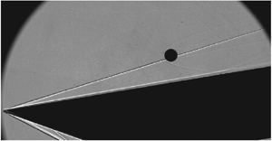Images were recorded with a Vision Research Phantom v2512, typically at 60 000 frames per second with $896\times 464$ pixel resolution and a $4\ \mathrm {\mu }\textrm {s}$ exposure time (though for the laser the effective exposure time was the $30\ \textrm {ns}$ pulse width). An example of a recorded image is shown in figure 8. The ramp oblique shock and boundary layer are clearly visible because of the extended line-of-sight integration length of these features, but the sphere bow shock is somewhat weaker. Despite the focusing set-up, some distortion of the sphere profile in the vicinity of the impingement point of the ramp shock is apparent. A weak viscous interaction is also evident near the leading edge of the ramp.

Figure 8. Example of a focused shadowgraph recorded during the experimental campaign.

The sphere motion was determined using the optical-tracking technique first developed in Laurence, Deiterding & Hornung (Reference Laurence, Deiterding and Hornung2007), and later refined in Laurence & Karl (Reference Laurence and Karl2010) and Laurence (Reference Laurence2012). In short, the sphere edge points in each image are located using a Canny pixel-resolution edge detector followed by subpixel localization. These points are then fitted in the least-squares sense with a circular profile, resulting in best-fit values for the sphere radius and the $(x,y)$ location of the sphere centre. The resulting position versus time profiles can then be differentiated numerically to obtain the sphere velocity, with some subsequent smoothing typically necessary because of the noise amplification intrinsic to numerical differentiation. Because of the optical distortion from the shock noted earlier, edge points near the intersection of the shock with the sphere outline were excluded from the fit (distortions of edge segments fully within the shock layer were found to be minimal).

For the present study, a key parameter is the normalized lateral distance from the sphere centre to the (extrapolated) oblique-shock location; thus, determining the shock position is also important. The visualized profile of the oblique shock shows the distinctive dark–bright pattern that one associates with shadowgraphy; the shock position at a given downstream location was thus assumed to lie at the interpolated point between the dark and light bands where the image intensity is equal to that of the background. Since the flow was non-uniform in the streamwise direction (diverging away from the centreline and increasing in Mach number), a constant shock angle was not assumed. Instead, a fourth-order polynomial was fitted to the locus of shock points detected throughout the duration of the relevant experiment. In general, accurately locating the shock was found to be somewhat more difficult towards the rear of the visualization region: the intensity gradients induced by the shock were typically weaker, and the shock there was more subject to oscillations. This latter effect became particularly pronounced for smaller spheres, where the oscillations were a larger fraction of the sphere diameters.

One further problem that the shadowgraph sequences revealed was the occurrence of particle impacts on the sphere during the test time, particularly for larger sphere diameters. Although the shock tunnel was thoroughly cleaned between each experiment, some degree of free-stream debris originating from the upstream diaphragms was unavoidable. Each visualization sequence was carefully examined for potential impacts, which resulted in the discarding of a number of experiments.

4.1. Sphere/oblique-shock interactions

In Part 1 of this work, we noted that the interactions of the sphere with the oblique ramp-generated shock should be dominated by inviscid effects, and thus that the force coefficients could be calculated to a good approximation under the inviscid assumption. To verify this, in figure 9 we compare inviscid coefficients calculated for a forced sphere interacting with the oblique shock generated by a $10^{\circ }$ ramp in Mach-6 flow using the AMROC code with equivalent viscous coefficients from the AERO software. In both cases, to minimize the effects of the sphere motion, the lift curves have been shifted so that they tend to zero in the free stream and scaled so that $L/D$ fully inside the shock layer is equal to the tangent of the ramp angle. We see that, for the two codes, both the lift and drag curves lie very close to one another. The most significant discrepancy is in the drag curves: neglecting the viscous contributions results in an underprediction of a few per cent (which also manifests itself in a slightly reduced lift inside the shock layer, since here a component of the drag is in the $y$ direction). There are also some small differences in the lift coefficients for the oblique shock impinging away from the sphere centre. The viscous free-stream drag coefficient is 0.92, which compares well with a value of 0.91 (${\pm }2\,\%$) documented by Bailey & Hiatt (Reference Bailey and Hiatt1971) for Mach numbers between 5.8 and 6.2 at an equivalent Reynolds number to the simulation here.

Figure 9. $(a)$ Comparison of (upper curves) drag and (lower curves) lift coefficients from (—) inviscid and (— —) viscous simulations. (b,d and c,e) Surface pressure and centreline Mach number from snapshots of (b,c) inviscid and (d,e) viscous solutions at (b,d) $(y-y_s)/r = 0$ and (c,e) $(y-y_s)/r = 0.6$.

We examine two points along the sphere traverses in additional detail to elucidate the flow features responsible for differences in the spheres’ surface pressures. Figure 9(b,d) provides a snapshot of both the inviscid (b) and viscous (d) flow fields at a sphere position of $(y-y_s)/r = 0$; the centreline Mach number is shown in grey scale (with sonic line highlighted), together with the surface pressure on the sphere. Note that, for presentation purposes, the surface pressure is extracted by interpolation of the fluid pressure onto a surface $1.02 r$ from the sphere's centre, which causes obscuration of the thin boundary layer in the viscous simulation. The lift and drag coefficients show minimal discrepancies at this point of the spheres’ traverse despite some differences in flow features. Both solutions seem to capture the type-IV shock–shock interaction with the embedded supersonic jet apparent in the Mach number visualizations, although its impingement location and width differ. The inviscid solution yields a narrower band of enhanced pressure at a lower location on the sphere's surface, which is likely a result of the opposite directions of travel in the simulations (the inviscid sphere is moving away from the ramp). Also, as expected, the inviscid solution lacks an extended wake, resulting in reduced base pressure relative to the viscous flow; however, this is not expected to contribute significantly to differences in the integrated surface pressure. In figure 9(c,e), we present Mach numbers and surface pressures for inviscid and viscous spheres at $(y-y_s)/r = 0.6$, where we see that the discrepancy in the lift curve is close to a maximum (note that different pressure normalizations have been used for the inviscid and viscous cases). Oblique-shock impingement here yields an augmented lift coefficient for the inviscid sphere, on whose inboard side appears a secondary region of high pressure (which also appears for the viscous simulation, but to a lesser degree). As before, this discrepancy likely stems from the differing directions of cross-range travel and an associated slight re-orientation of the sphere bow shock. Such a small geometric change is nevertheless apparently sufficient to modify the class of shock–shock interaction, as evidenced by the pocket of subsonic flow immediately downstream of the intersection in only the inviscid interaction. Despite this qualitative difference, the discrepancy in lift coefficient is minor and that in the drag coefficient negligible. Overall then, we conclude that using inviscid simulations to compute force coefficients for the sphere–shock interactions at these conditions is well justified.

4.2. Near-wall flow features and sphere forces

We now turn our focus to the VULCAN simulations and the interactions between a sphere and a high-speed boundary layer. A series of representative visualizations for the $4$, $6$ and $8\ \textrm {mm}$ diameter spheres ($r/\delta =2.67$, 4 and 5.33) are shown in figure 10: in each case, a streamwise numerical schlieren is shown on a plane through the sphere centreline, the wall-normal temperature gradient (i.e. heat flux) is visualized on the wall surface, and the sphere surface is coloured by pressure.

Figure 10. Numerical visualizations from the viscous sphere/boundary-layer simulations: (a–d) 4 mm diameter sphere ($r/\delta =2.67$) at $y/r= (a)\, 1.125$, (b) 1.375, (c) 1.625 and (d) 2.125; (e–h) 6 mm diameter sphere ($r/\delta =4$) at $y/r=\,(e)\,1.083$, (f) 1.250, (g) 1.417 and (h) 1.917; and (i–l) 8 mm diameter sphere ($r/\delta =5.33$) at $y/r=\,(i)\, 1.063$, (j) 1.188, (k) 1.4 and (l) 1.8. In each visualization, a schlieren plane through the sphere centreline is shown, together with pressure contours on the sphere surface. The wall is coloured according to the calculated wall-normal temperature gradient.

For the $4\ \textrm {mm}$ sphere at $y/r=1.125$ (the nearest-wall position investigated), the boundary layer separates approximately 7.2 radii upstream. As depicted in figure 10(a), this creates a situation in which the sphere lies entirely within the separation-shock layer, with a type-V interaction between the sphere bow shock and the separation shock. For the nearest wall $6\ \textrm {mm}$ and $8\ \textrm {mm}$ cases (figure 10e,i), the separation shock impinges on the upper sphere surface, despite these computations having been carried out for slightly smaller values of $y/r$. Nevertheless, all three cases exhibit similar fluid structures within the separated region that closely resembles those computed by Tutty et al. (Reference Tutty, Roberts and Schuricht2013) for hypersonic flow around a blunted fin–body junction. Note, for example, the secondary separation regions and associated vortices within the primary separation zone that manifest themselves as curved heat-flux features on the wall. Beyond this initial near-wall spacing, the flow features for all three sphere diameters evolve in similar fashion, but for different values of $y/r$. As the sphere is displaced further from the wall, as in figure 10(b,f,j), it imposes less blockage on the boundary layer, allowing the boundary-layer separation point to move downstream; however, the shock–shock interaction is now a stronger type-IV, resulting in elevated pressure near the sphere nose. By figure 10(c,g,k) in each case, the separation-shock interaction has developed towards type-III, wetting only the lower half of the sphere with doubly shocked flow, but nevertheless producing a localized high-pressure region there (which we would expect to contribute primarily to the lift coefficient). For larger wall-normal displacements, the only remaining wall influence comes from a type-II or type-I interaction (or a wake interaction), which will but weakly affect the sphere aerodynamics.

Figure 11 shows the lift and drag coefficients determined in the viscous simulations, plotted versus $y/r$ for all sphere diameters; these are also compared to results from a forced inviscid (AMROC) simulation of a sphere interacting with a reflecting boundary at the same Mach number. We see that the force coefficients are altered dramatically by the presence of the wall boundary layer. Most notable is the effect on the lift coefficient for small diameters: rather than the repulsive forces seen in Part 1, the lateral force is close to zero for the $d=6\ \textrm {mm}$ sphere, and for the $d=4\ \textrm {mm}$ sphere it is attractive in the immediate vicinity of the wall. As $y/r$ increases for both these cases, $C_L$ trends upwards, becoming weakly positive before necessarily reverting back to zero sufficiently far from the wall. The $d=8\ \textrm {mm}$ case demonstrates the beginning of a trend reversal close to the wall, as the lift is already positive near the wall and rises to only a slight peak at $y/r=1.6$ before dropping to zero. Increasing the sphere diameter to $d=12\ \textrm {mm}$ shows a continuation of this trend reversal: the lift clearly peaks near the wall and drops more rapidly as $y/r$ is increased. This behaviour is to be expected considering that, as $r/\delta$ increases, the boundary-layer length scale becomes insignificant and the solution must approach the inviscid limit. As for the drag coefficient, the effect of the boundary-layer interaction near the wall is to reduce $C_D$ slightly relative to the inviscid solutions. As $C_L$ increases with $y/r$ for the $4$, $6$ and $8\ \textrm {mm}$ simulations, $C_D$ also shows a small increase (to ${\sim }1.05$), before falling back to the free-stream value of 0.94. The latter number compares with a value of 0.92 (${\pm }2\,\%$) as given by Bailey & Hiatt (Reference Bailey and Hiatt1971) for Mach numbers between 4.8 and 5.2 and similar Reynolds numbers to the computations; considering the slightly lower Mach number here, this can be considered acceptable agreement. Increasing the sphere diameter to $12\ \textrm {mm}$ once again reveals a near-wall trend reversal: the drag has begun to qualitatively resemble the inviscid trend with a clear maximum lying very near the wall, although recovery to the free-stream value is still significantly delayed. Overall, these simulations demonstrate that the influence of the wall is felt significantly farther away than in the inviscid computations, particularly for smaller sphere diameters.

Figure 11. $(a)$ Lift and $(b)$ drag coefficients of a sphere near a viscous wall at Mach 4.65 as functions of normalized distance from the wall: (—) inviscid; ($\blacktriangle$) $d=4\ \textrm {mm}$, $r/\delta =2.67$; ($\bullet$) $d=6\ \textrm {mm}$, $r/\delta =4$; ($\blacksquare$) $d=8\ \textrm {mm}$, $r/\delta =5.33$; ($\blacklozenge$) $d=12\ \textrm {mm}$, $r/\delta =8$; and ($\blacktriangledown$) $d=16\ \textrm {mm}$, $r/\delta =10.67$. The dashed lines are interpolated curves between the discrete computed points.

To obtain a better understanding of the near-wall aerodynamic trends in figure 11, two additional flow visualizations are shown in figure 12 for the $d= 4$ and $16\ \textrm {mm}$ cases, where the off-wall spacing is $0.25\ \textrm {mm}$ for each (i.e. $y/r=1.125$ and 1.031). The length scale of each image has been normalized based on sphere radius and the wall visualization has been removed to improve visibility of the pressure distribution on the underside of the spheres; sonic lines have also been superimposed on the numerical schlieren to distinguish regions of subsonic and supersonic flow. Additionally, in the right graph of the figure we have plotted the pressure profile along the sphere centreline in each case. For both sphere diameters, the interaction with the separation shock appears to shift the peak pressure slightly to the upper side of the sphere, and this is confirmed in the pressure plots. This shift will produce a negative lift contribution, which is more than offset in the $d=16\ \textrm {mm}$ case by a region of high pressure on the underside of the sphere (peaking at around $-70^{\circ }$). For the $d=4\ \textrm {mm}$ sphere, however, this underside pressure peak is much reduced, probably because of the reduced fluid momentum in the boundary layer. The overall lift coefficient is thus dominated by the nose region and becomes negative, in contrast to the larger sphere. The pressure levels on the smaller sphere are also generally lower, leading to the reduced drag coefficient.

Figure 12. (a,b) Flow visualizations for the $d=4\ \textrm {mm}$ ($r/\delta =2.67$) and $16\ \textrm {mm}$ ($r/\delta =10.67$) sphere cases, each with an off-wall spacing of $0.25\ \textrm {mm}$ ($y/r=1.125$ and 1.031); sonic lines are overlaid in blue. $(c)$ Sphere centreline pressures for these two cases: ($\blacktriangle$) $r/\delta =2.67$; ($\blacktriangledown$) $r/\delta =10.67$ ($\theta <0$ is the near-wall hemisphere).

The accelerated recovery of the aerodynamic coefficients to their free-stream values for larger spheres can be attributed to a reduction in the relative size of the separated region. This trend can be seen in figure 13, where we have plotted the separation length (normalized by the sphere radius) versus the normalized wall-normal displacement. The separation point is determined as the most upstream location at which the streamwise wall shear stress drops below zero; we then define the separation length as the streamwise distance between the separation point and the centre of the sphere. A clear trend is observed for the normalized separation length to decrease with increasing sphere diameter. Thus, assuming that the separation-shock angle does not change with sphere diameter, the impingement point of this shock on the sphere will be swept off the sphere surface earlier (at smaller $y/r$) for larger spheres, explaining the observed trend.

Figure 13. Normalized separation length as a function of $y/r$ for: ($\blacktriangle$) $r/\delta =2.67$; ($\bullet$) $r/\delta =4$; ($\blacksquare$) $r/\delta =5$.33; ($\blacklozenge$) $r/\delta =8$; and ($\blacktriangledown$) $r/\delta =10.67$.

4.3. Trajectory modelling

We have seen that the sphere force coefficients near the wall can differ markedly if a boundary layer is present, and we wish to gain insight into the effects on the sphere separation behaviour that this might have. This will also assist in interpreting the experimental results described in § 5. In order to make approximate predictions, we employ the viscous force coefficients from VULCAN within a decoupled methodology as was described in Part 1 of this work. The procedure employed is as follows. First, for a given $r/\delta$, we interpolate between the discrete computed $C_L$ and $C_D$ values to create continuous functions of $y/r$ for the viscous wall interactions. These interpolated curves are shown together with the discrete computed values in figure 11. With these coefficient profiles specified for a flat-plate flow, it is straightforward to transform to the coefficients that would be experienced by the sphere near the surface of an inclined ramp (assuming the ramp-generated shock to be well away from the sphere, and that the post-shock Mach number is the same as that of the free stream in the original flat-plate computation); this is accomplished by a simple rotation (by the ramp angle) and a rescaling of the dynamic pressure (so that it is representative of the pre-shock conditions).

The decoupled model amounts to assuming that the sphere–wall interactions just described and the sphere–shock interactions contribute independently to the force coefficients. Considering the minimal differences between the inviscid and viscous coefficients for the sphere–shock interactions noted in § 4.1, it is appropriate to use inviscid AMROC simulations to determine the latter contributions, as in Part 1 of this work; to ensure consistency, however, we scale the undisturbed inviscid drag coefficients so as to match the viscous values. In this manner, we can construct full force-coefficient profiles as functions of $y/r$ for any downstream location, and by integrating the equations of motion using these profiles, we can derive trajectory predictions. Note, however, that the decoupled assumption will be more approximate here than in the inviscid situation examined in Part 1. First, the wall force-coefficient profiles are interpolated rather than computed directly. Second, figure 10 shows that when the sphere is close to the wall, the induced separation shock can extend above the top of the sphere; this is in contrast to the inviscid case, for which the wall effects were restricted to the lower part of the sphere, and will mean that it is less valid to treat the sphere–wall and sphere–shock effects independently. Last, as the sphere separates from the wall, it will also move along the ramp, meaning that the local boundary-layer thickness will increase. In the decoupled model, however, we effectively treat this thickness as constant (though, since the boundary-layer growth is slow, this will not be a major concern). In light of these points, the decoupled predictions in this subsection should be considered qualitative indications of the sphere behaviour rather than rigorous predictions.

Figure 14 shows trajectories for several starting locations calculated using this decoupled approach and the $r/\delta =2.67$ viscous-wall coefficients; trajectories are shown (i) in physical space ($y/r$ versus $x/r$), (ii) in terms of the normalized distance of the sphere from the shock, $(y-y_s)/r$, versus normalized distance downstream and (iii) in the $\eta -v_\eta$ phase plane. Here, $\eta =(y-y_s)/r$ and $v_\eta ={\rm d}\eta /{\rm d}\hat {t}=\hat {v}_y-\tan \beta \hat {v}_x$, where $\hat {v}_x=\sqrt {\rho _b/\rho _a}v_x/V$, $\hat {v}_y=\sqrt {\rho _b/\rho _a}v_y/V$ are the normalized streamwise and lateral velocities, and $\hat {t}=\sqrt {\rho _a/\rho _b}Vt/r$ is the normalized time; $\rho _b$ and $\rho _a$ are the sphere and free-stream gas densities and $V$ the free-stream velocity. Employing such a phase-plane analysis was shown in Part 1 of this work to be highly useful for understanding the sphere dynamics. All trajectories start on the $v_\eta =0$ axis; shifting the release location downstream corresponds to decreasing the starting value of $\eta$. Since we are assuming constant $r/\delta$, the different trajectories shown should not strictly be thought of as corresponding to simply moving the sphere along the ramp to different release locations while maintaining constant inflow conditions (as in the experiments); instead, either the sphere radius or the Reynolds number would need to be correspondingly adjusted to maintain a constant $r/\delta$. In all these trajectories, we see that the negative lift (suction) close to the wall dominates the sphere behaviour, resulting in direct entrainment for all release locations. For the trajectories that start close to the ramp leading edge, the positive lift generated by the sphere–shock interactions enable the sphere to ride the shock a short distance downstream; however, the negative change in $v_\eta$ produced in interacting with the wall means that even these trajectories are pushed out of the stable region in the phase plane, and the sphere becomes entrained within the shock layer. Releasing further downstream essentially results in the sphere simply moving along the wall (which we may consider a special case of the direct-entrainment trajectory type). As we would expect the viscous lift coefficients to become increasingly negative for small $r/\delta$ values, we conclude that direct entrainment is the dominant behaviour for smaller spheres.

Figure 14. $(a)$ Calculated separation trajectories in physical space for a Mach-6 free stream and a ramp angle of $10^{\circ }$, using the wall force coefficients for $r/\delta =2.67$ and starting locations of $x_0/r=5$, 7, 9, 11, 12.5 and 13; $(b)$ trajectories plotted as normalized distance from the shock versus $x/r$, with the dashed lines indicating the locations of the stationary points; $(c)$ trajectories in the phase plane, with the separatrix indicated by the dashed line and the centre stationary point by the $\times$.

Figure 15 shows equivalent results using the $r/\delta =4$ viscous-wall coefficients. In this case we observe much more interesting behaviour than previously. Near the wall, the viscous lift coefficient is close to zero and the drag is only slightly enhanced, meaning that the trajectories in the phase plane are not too different from those the sphere would follow if the wall were not present at all. As a result, the majority of the trajectories that begin in the stable region indicated by the closed dashed line (i.e. those that begin relatively close to the leading edge) remain in this region as the sphere separates from the wall, producing surfing behaviour in these cases. The reader is reminded that, for an inviscid wall with this combination of ramp angle and Mach number as examined in Part 1, surfing was not found to be possible: all derived trajectories were of the expulsion/re-entrainment or direct-entrainment types. We thus see that, at least under certain circumstances, viscous effects are enabling for surfing behaviour. As the starting location is translated downstream, there is still a small range of positions for which expulsion/re-entrainment trajectories result ($x_0/r$ values between 10.1 and 11.8). This is because of the slightly positive lift coefficient (and negligible drag enhancement) characteristic of the $r/\delta =4$ curves a small distance from the wall; this lift enhancement acts to push the sphere outside the stable region for trajectories when it would otherwise have been close to the boundary. Overall, however, the dominant behaviours for this set of viscous-wall coefficients are surfing (for relatively small $x_0/r$) and direct entrainment (for larger $x_0/r$).

Figure 15. $(a)$ Calculated separation trajectories in physical space for a Mach-6 free stream and a ramp angle of $10^{\circ }$, using the wall force coefficients for $r/\delta =4$ and $x_0/r=5$, 7, 9, 11, 12.5, and 13 (as in figure 14); $(b)$ trajectories plotted as normalized distance from the shock versus $x/r$; $(c)$ trajectories in the phase plane.

Corresponding trajectories for the $r/\delta =5.33$ viscous-wall coefficients are shown in figure 16. As noted earlier, these coefficients have an increased tendency towards the inviscid profiles and this is reflected in the sphere behaviour. For starting locations near the ramp leading edge, surfing remains possible (in contrast to the inviscid case), but from $x_0/r=8.8$ the ejection/re-entrainment-type trajectories that predominated in inviscid flow for these conditions are observed. This behaviour transitions to direct entrainment for starting locations from $x_0/r=12.6$, a short distance downstream of the saddle point.

Figure 16. Calculated separation trajectories for a Mach-6 free stream and a ramp angle of $10^{\circ }$, using the wall force coefficients for $r/\delta =5.33$ and $x_0/r=5$, 7, 9, 11, 12.5, and 13 (as in figure 14); $(a)$ trajectories plotted as normalized distance from the shock versus $x/r$; $(b)$ trajectories in the phase plane.

The computed viscous-wall coefficients will be valid not only for the combination of a Mach-6 flow with a $10^{\circ }$ ramp examined thus far, but also for other combinations of free-stream Mach number and ramp angle that produce a Mach-4.65 post-shock flow. In Part 1 of this work, it was found that the relative predominance of surfing could depend strongly on each of these parameters. Therefore, to gain insight into the separation problem for another set of flow conditions, trajectories for an $18^{\circ }$ ramp in a Mach-10 flow (post-shock Mach number 4.60) were also calculated for the various sphere diameters; the results are shown in figures 17 and 18. In general, increasing the Mach number and ramp angle causes the force coefficients generated by the sphere–shock interactions to grow significantly (see Part 1), and we might thus expect the sphere–shock interactions to dominate increasingly over the sphere–wall interactions. This is indeed seen in these sphere trajectories, which for the most part show only minor differences from if the wall were absent. In particular, surfing and direct-entrainment behaviours are predominant, with only a limited range of release locations leading to ejection/re-entrainment (a trajectory type that is only possible because of wall interactions). Otherwise, the influence of the wall is seen most strongly in the $r/\delta =2.67$ trajectories of figure 17. The transition to direct entrainment occurs here slightly upstream of the saddle point (because of wall suction), but more interestingly, for release positions close to the leading edge (near the centre location), the wall suction is sufficient to drag the sphere out of the stable region, also resulting in direct entrainment. Note, however, that here the decoupled assumption will be highly questionable, so it is not clear that such trajectories would be observed in reality.

Figure 17. $(a)$ Calculated separation trajectories in physical space for a Mach-10 free stream and a ramp angle of $18^{\circ }$, using the wall force coefficients for $r/\delta =2.67$ and $x_0/r=4$, 5, 7, 11, 15, 17, and 19; $(b)$ trajectories plotted as normalized distance from the shock versus $x/r$; $(c)$ trajectories in the phase plane.

Figure 18. Phase-plane trajectories for an $18^{\circ }$ ramp in Mach 10 flow using the wall force coefficients for $(a)$ $r/\delta =4$ and $(b)$ $r/\delta =5.33$. The release locations in both cases are $x_0/r=5$, 9, 13, 15, 17, 18 and 19.

5.1. Shock-surfing phenomenon

From the experiments, we first wish to verify that surfing behaviour is indeed possible for the configuration employed (in particular the combination of a $10^{\circ }$ ramp angle with a Mach ${\sim }6$ flow). In the hanging sphere tests, the sphere was initially positioned in the undisturbed free stream; its trajectory would subsequently take it through the shock and into the shock layer, enabling a full range of force coefficients to be calculated as functions of normalized lateral distance from the shock, $(y-y_s)/r$. A visualization sequence from one such experiment is shown in figure 19, together with the force coefficients and lift-to-drag ratios calculated from three experiments. While some variation is present between the experimental results, the trends are consistent with each other and with the numerical curves shown in § 4.1. In the $L/D$ curves, in all cases we see that the peak $L/D$ exceeds the tangent of the shock angle ($\beta$ was calculated directly from the visualizations). This is both a necessary and sufficient condition for surfing to be possible, indicating that we should be able to observe this phenomenon at the present conditions. To verify this, an experiment was conducted in which a 1.59 mm diameter sphere was initially placed directly on the oblique shock (i.e. nominally within the stable region) at the ramp leading edge. The sphere's trajectory can be seen in the sequence of shadowgraph images in figure 20. Surfing of the shock is clearly observed (note, for example, that in the second and fourth images the sphere is close to its maximum and minimum penetration into the shock layer), demonstrating that our prediction of the possibility of this phenomenon is indeed accurate here.

Figure 19. $(a)$ Sequence of shadowgraph images showing the passage of an initially hanging sphere through the ramp-generated oblique shock. $(b)$ Derived drag (—) and lift (— —) coefficients for three such hanging sphere tests (thin coloured lines) together with fitted profiles (thick black lines) based on the computed viscous coefficients. $(c)$ Lift-to-drag ratio for the three hanging experiments; the dashed horizontal line indicates the average value of $\tan \beta$ calculated from the visualizations.

Figure 20. Experimental shadowgraph sequence showing the trajectory of a 1.59 mm diameter sphere released near the ramp's leading edge.

In figure 19(b), we have also plotted fitted coefficient curves based on the viscous computations described in § 4.1; these have been shifted, scaled and stretched to best match the average experimental curve. These coefficient profiles will be used in the next subsection to assist in interpreting the shedding experiments.

5.2. Shedding behaviour

Visualization sequences for 3.18 mm and 9.53 mm diameter spheres released from the ramp surface are shown in figures 21 and 22, respectively, and the derived sphere trajectories over the sets of experiments for these two sphere diameters are plotted in figure 23. Supplementary movies of several cases are available at https://doi.org/10.1017/jfm.2020.757. For all sphere diameters, the general trend as the release location is shifted downstream along the ramp is as would be expected from § 4.3: for relatively upstream starting locations, either surfing or ejection/re-entrainment was observed (though it could be difficult to distinguish between these two trajectory types purely from the visualizations as, particularly for larger spheres, there was not sufficient downstream length for a full oscillation about the shock to be completed), transitioning to direct entrainment at some critical distance downstream. Note that, even for the largest, 9.53 mm diameter sphere, if the release location was far enough downstream, the sphere would simply move along the ramp surface, indicating the lift coefficient in the ramp-aligned coordinate system to be less than or equal to zero.

Figure 21. Sequences of shadowgraph images showing a 3.18 mm diameter sphere released from the surface of the ramp at $(a)$ $x_0/r=3.9$ and $(b)$ $x_0/r=9.1$. The temporal spacing between images is $(a)$ $862\ \mathrm {\mu }\textrm {s}$ and $(b)$ $627\ \mathrm {\mu }\textrm {s}$.

Figure 22. Sequences of shadowgraph images showing a 9.53 mm diameter sphere released from the surface of the ramp at $(a)$ $x_0/r=10.4$ and $(b)$ $x_0/r=11.0$. The temporal spacing between images is $(a)$ $813\ \mathrm {\mu }\textrm {s}$ and $(b)$ $869\ \mathrm {\mu }\textrm {s}$.

Figure 23. Experimentally measured sphere trajectories in normalized physical space for $(a)$ 3.18 mm and $(b)$ 9.53 mm diameter spheres.

To obtain a more comprehensive picture of the sphere behaviour in the different cases, trajectories determined for the 3.18 mm, 6.35 mm and 9.53 mm diameter spheres are shown in $x/r$–$\eta$ space and the $\eta$–$v_\eta$ phase plane in figure 24. In the $x/r$–$\eta$ graphs, the locations of the two stationary points are indicated by horizontal dashed lines, while in the phase-plane plots we have included a calculated separatrix to assist in interpreting the trajectories. The stationary-point locations and separatrix profile were calculated based on the fitted coefficient curves shown in figure 19(b). The experimental results are also summarized in table 6, where we have provided $x_0/r$ values and corresponding estimates of $r/\delta$, together with indications of the trajectory type. The boundary-layer thickness here, $\delta$, is the 99 %-velocity thickness determined from VULCAN simulations of the experimental set-up, the details of which are included in the Appendix.

Figure 24. Experimentally measured sphere trajectories plotted ($a{,}c{,}e$) as $\eta =(y-y_s)/r$ versus $x/r$ and ($b{,}d{,}f$) in the $\eta-$$v_\eta$ phase plane for sphere diameters of (a,b) $3.18\ \textrm {mm}$, (c,d) $6.35\ \textrm {mm}$ and (e,f) $9.53\ \textrm {mm}$. In ($a{,}c{,}e$), the dashed lines indicate the locations of the computed stationary points and, in ($b{,}d{,}f$), the profile of the computed separatrix.

Table 6. Summary of shedding experiments performed.

For the 3.18 mm diameter spheres, the most upstream release location ($x_0/r=3.9$) clearly results in a surfing trajectory, with the phase-plane orbit well within the stable region bounded by the separatrix. The nature of the $x_0/r=6.7$ trajectory is more ambiguous as it almost coincides with the separatrix curve; ejection/re-entrainment appears to be the most likely outcome here, although surfing may also be possible. In any case, for the next most downstream release location ($x_0/r=7.2$), we appear to be back to surfing behaviour, with the trajectory lying wholly within the stable region of the phase plane (we attribute the apparent crossing of the $x_0/r=3.9$ trajectory to difficulties in precisely locating the shock position, as noted in § 5.1). A progression from surfing to ejection/re-entrainment and then back to surfing with increasing $x_0/r$ was not observed in the simulated trajectories of § 4.3 (where ejection/re-entrainment always transitioned to direct entrainment), but here we have the added complexity of a decreasing $r/\delta$ with increasing $x_0/r$, which will lead to increased wall suction for larger values of $x_0/r$, and could explain the observed behaviour (as this suction will act against the tendency towards initial ejection). For $x_0/r=7.9$ and above, the sphere is directly entrained.

For the 6.35 mm diameter spheres, the two most upstream release locations result in ejection/re-entrainment, although the $x_0/r=9.5$ case appears to be right on the boundary with direct entrainment; at $x_0/r=10$, we clearly see transition to the latter trajectory type. For the largest, 9.53 mm diameter spheres, we again observe a surfing trajectory at the most upstream release location ($x_0/r=7.7$). This transitions to ejection/re-entrainment moving downstream to $x_0/r=9.5$ and 10.4 (although for $x_0/r=9.5$, the phase-plane trajectory appears to enter the stable region from outside towards the end of the observed sphere motion – we again attribute this to difficulties in accurately locating the shock position towards the rear of the shadowgraph visualization region). A transition to direct entrainment is then obtained between $x_0/r=10.4$ and 11.0.

Comparing the three sphere diameters, we see a clear trend for the $x_0/r$ value at which transition to direct entrainment occurs to move further downstream as the sphere diameter is increased. This trend was present in the numerical predictions of § 4.3, but is even more pronounced here. A contributing factor may be the viscous interaction noted earlier in the shadowgraph images. This will push the shock location out further from the ramp, resulting in smaller $\eta$ values at a given $x_0/r$ than would be predicted by inviscid shock theory (as was employed in § 4.3); however, since the viscous interaction acts near the leading edge, its effects will be less significant for release locations farther downstream. We can also compare select experimental results with the numerical predictions, again focusing on the transition $x_0/r$ to direct entrainment (with the caveat of slightly different free-stream Mach numbers). For the 3.18 mm diameter sphere, we see that this transition occurs at an $r/\delta$ value of approximately 3.8, which facilitates a comparison with the predictions based on the viscous force coefficients for the 6 mm diameter sphere. We note that the transition occurs at a somewhat smaller value of $x_0/r$ in the experiment – between 7.2 and 7.9, as compared to 11.8 in the simulation (which is in fact larger than the transition $x_0/r$ for the largest sphere in experiments). This is again consistent with the influence of the viscous interaction displacing the shock to larger $y_s$ in experiments and thus decreasing the effective value of $\eta$ at the release location.