


1 Introduction
Fluid lubricated bearings utilise a thin fluid film to maintain a clearance between two structural components, a rotor and stator, when experiencing an axial load, typically through a hydrodynamic force generated by the dynamic motion of the bearing faces to enhance the local fluid film pressure. Current bearing technology provides a significant improvement in bearing efficiency for applications characterised by higher operating speeds and maintenance of smaller clearances.
An early theoretical study by Taylor & Saffman (Reference Taylor and Saffman1957) examined the axial motion and air flow through a coaxial parallel rotor and stator separated by a thin air film. A bearing model was derived from the compressible Navier–Stokes equations on neglecting rotational inertia and considering small amplitude disturbances. Predictions accurately simulated experimental results, confirming the existence of a squeeze film force due to air compressibility.
To capture the dynamics of a coupled bearing model, the fluid flow needs to be appropriately coupled to the bearing structure. Three-dimensional motion of a fluid lubricated device was modelled by Etison (Reference Etison1980), and the hydrodynamic and hydrostatic components of the air film pressure were identified; the squeeze film pressure was incorporated into the hydrostatic component. Results show the squeeze film behaviour can potentially be used to maintain the air film between the rotor and stator. For highly vibrating operational environments, Salbu (Reference Salbu1964) examined the possibility of significant disturbances in the axial direction through theoretical analysis and associated experimental investigations. The rotor–stator clearance corresponds to an oscillatory motion and results confirm a load carrying capacity for squeeze films with the pressure and force in the air film increasing with the amplitude of the axial oscillations.
More recently, Garratt et al. (Reference Garratt, Cliffe, Hibberd and Power2012) examined the dynamics of the coupled fluid–structure interaction of a high-speed air lubricated bearing (compressible flow) with parallel faces where the effect of centrifugal inertia, which is typically neglected in bearing configurations, was included. The bearing dynamics was investigated in the case of the lower face (rotor) undergoing prescribed periodic axial oscillations with an amplitude smaller than the equilibrium fluid film thickness. The upper face (stator) can have axial motion as a rigid displacement in response to the induced film motion by the moving rotor, with the stator dynamics modelled as a spring–mass–damper system. Following the approach of Garratt et al. (Reference Garratt, Cliffe, Hibberd and Power2012), Bailey et al. (Reference Bailey, Cliffe, Hibberd and Power2013) considered the case of a liquid lubricated bearing (incompressible flow) with a coned rotor shape, usually designed to increase the lubrication forces between the faces (stability studies by Etison (Reference Etison1980) identify optimal coning angles for a range of practical bearing configurations). Analysis by Bailey et al. (Reference Bailey, Cliffe, Hibberd and Power2013) included the possibility of rotor axial disturbances having an amplitude larger than the equilibrium film thickness. Under these conditions, results indicate that the lubrication force can always prevent the possibility of contact. Although, in both cases (parallel and coned bearing) the fluid gap can become very small, even of the order of nano-scale, leading to the possible invalidation of the classical no-slip velocity condition. A slip boundary condition of the Navier type is incorporated in the analysis by Bailey et al. (Reference Bailey, Cliffe, Hibberd and Power2014, Reference Bailey, Cliffe, Hibberd and Power2015) in cases of parallel and coned liquid lubricated bearings, respectively. The obtained results indicate that face contact does not occur in parallel bearings; however, the bearing gap can become very small. On the other hand, possible face contact can occur in the case of a coned bearing for some critical values of the magnitude of the rotor oscillation, conical angle and slip length. In this last case, the desired effect of the conical angle on the lubrication force is mitigated by the slip flow and classical design criteria are debatable.
Due to efficiency and environmental considerations, modern bearing and sealing designs have been characterised by extremely small gaps, even of the order of several microns (almost contact designs). Of significant importance is the analysis of the fluid structure coupling dynamics of such bearings working under extreme conditions, where possible disturbances can displace the rotor to magnitudes larger than the initial equilibrium film thickness. In this work, air bearings with a small face clearance are analysed to examine their dynamical behaviour, extending the study of incompressible flow bearings with a slip condition by Bailey et al. (Reference Bailey, Cliffe, Hibberd and Power2014, Reference Bailey, Cliffe, Hibberd and Power2015) to compressible flow. In the case of incompressible flow, it is possible to obtain an analytical solution of the corresponding linear Reynolds equation for the pressure field, enabling the coupled bearing problem to be formulated as a single second-order non-autonomous ordinary differential equation for the bearing gap. Also the asymptotic solution at a small gap condition can be found and used to verify the numerical results of the complete dynamic behaviour of the bearing when near contact conditions are predicted (for more details see Bailey et al. (Reference Bailey, Cliffe, Hibberd and Power2013, Reference Bailey, Cliffe, Hibberd and Power2014, Reference Bailey, Cliffe, Hibberd and Power2015)). Unfortunately in the present case of compressible flow, due to the nonlinear form of the resulting Reynolds equation, this approach is not easy to implement. For this reason in the present work only numerical solutions of the corresponding nonlinear problem are considered and the proposed numerical scheme is verified in the limit when the flow field tends to behave as incompressible flow.
A study by Taylor & Saffman (Reference Taylor and Saffman1957) indicated compressibility effects may be of importance when a fluid is forced into a narrow space and confirmed a compressible flow model gives the best correspondence with experimental work for an air lubricated bearing. Parkins & Stanley (Reference Parkins and Stanley1982) examined the effects of compressibility on the bearing dynamics by comparing experimental results with a coupled model for an oil squeeze film bearing. Although their model agreed reasonably with experimental results for some cases, examination over a range of cases revealed limitations due to neglecting compressibility effects. Conditions for compressibility effects to be neglected for bearing flow have previously been derived by Bailey et al. (Reference Bailey, Cliffe, Hibberd and Power2014); the conservation of mass reduces to the statement of solenoidal velocity field and the compressible flow in the bearing behaves as if it were incompressible flow for sufficiently small radial and azimuthal speeds.
In this study, we extend the work of Garratt et al. (Reference Garratt, Cliffe, Hibberd and Power2012) on air lubricating bearings by incorporating an analysis for a very small face clearance (at the micro-scale), where the classical no-slip boundary condition may be invalidated and instead boundary slip needs to be taken into account. The importance of this type of analysis for bearing/seal dynamics has been highlighted by Sayma et al. (Reference Sayma, Bréard, Vahdati and Imregun2002) in a numerical study on the seal mechanics. It was observed that for gaps of the order of
 $10~\unicode[STIX]{x03BC}\text{m}$
, typical of some hydrodynamic seals, steady-state solutions of the Navier–Stokes system of equations with no-slip boundary conditions are not possible to find. In such cases, the flow has a high Knudsen number and the mathematical formulation used for the problem may no longer be valid, requiring rarefied gas dynamics to be considered.
$10~\unicode[STIX]{x03BC}\text{m}$
, typical of some hydrodynamic seals, steady-state solutions of the Navier–Stokes system of equations with no-slip boundary conditions are not possible to find. In such cases, the flow has a high Knudsen number and the mathematical formulation used for the problem may no longer be valid, requiring rarefied gas dynamics to be considered.
The surface-to-volume ratio increases dramatically when flow geometries are scaled down to micro-/nano-scales. In these conditions, surface related phenomena become increasingly dominant, and new flow features can arise from the interactions between the fluid flow constituents and the solid surfaces that contain them. A phenomenon known as the slip flow condition could emerge as a consequence of an insufficient number of molecules in the sampling region, see Gad-el-Hak (Reference Gad-el-Hak2006). The characteristics of the flow is determined by the Knudsen number,
 $Kn=\tilde{\unicode[STIX]{x1D706}}/h$
, with
$Kn=\tilde{\unicode[STIX]{x1D706}}/h$
, with
 $\tilde{\unicode[STIX]{x1D706}}$
as the mean free molecular path (collision distance between molecules; for air at atmospheric conditions
$\tilde{\unicode[STIX]{x1D706}}$
as the mean free molecular path (collision distance between molecules; for air at atmospheric conditions
 $\tilde{\unicode[STIX]{x1D706}}=68~\text{nm}$
) and
$\tilde{\unicode[STIX]{x1D706}}=68~\text{nm}$
) and
 $h$
as the characteristic fluid thickness. For small Knudsen number (
$h$
as the characteristic fluid thickness. For small Knudsen number (
 $Kn<10^{-3}$
), the fluid is considered as a continuum with no-slip boundary conditions. For a larger Knudsen number between
$Kn<10^{-3}$
), the fluid is considered as a continuum with no-slip boundary conditions. For a larger Knudsen number between
 $10^{-3}$
and
$10^{-3}$
and
 $10^{-1}$
, a continuum model with a slip boundary condition is usually employed (slip flow regime); this is the flow regime of interest in the present work. For Knudsen number between
$10^{-1}$
, a continuum model with a slip boundary condition is usually employed (slip flow regime); this is the flow regime of interest in the present work. For Knudsen number between
 $10^{-1}$
and
$10^{-1}$
and
 $10$
, the flow is in a transition region and a modified continuum model needs to be considered. Finally for larger values (
$10$
, the flow is in a transition region and a modified continuum model needs to be considered. Finally for larger values (
 $Kn>10$
), molecular dynamics can be employed to describe the free molecular flow, for more details see Karniadakis, Beskok & Aluru (Reference Karniadakis, Beskok and Aluru2005). Under specified ambient condition, i.e. for a given value of
$Kn>10$
), molecular dynamics can be employed to describe the free molecular flow, for more details see Karniadakis, Beskok & Aluru (Reference Karniadakis, Beskok and Aluru2005). Under specified ambient condition, i.e. for a given value of
 $\tilde{\unicode[STIX]{x1D706}}$
, the value of the Knudsen number is determined by the characteristic length scale of the gas flow.
$\tilde{\unicode[STIX]{x1D706}}$
, the value of the Knudsen number is determined by the characteristic length scale of the gas flow.
Navier (Reference Navier1829) was the first to propose a slip model based on a linear relationship between the tangential shear rate and the fluid–wall velocity difference, i.e. a jump velocity at the wall is linearly proportional to the first-order derivatives of the fluid velocity with a proportionality constant given by the slip length (first-order model). This type of first-order slip model has been implemented for many different types of slip flow successfully reproducing flow characteristics in the slip regime, see Gad-el-Hak (Reference Gad-el-Hak2006), Wei & Yogendra (Reference Wei and Yogendra2007), Nieto, Giraldo & Power (Reference Nieto, Giraldo and Power2011). Higher-order slip models, where the jump velocity at the walls is also proportional to higher-order derivatives of the fluid velocity, have been proposed in the literature to extend slip flow predictions into the transition regime (for more details see Zhang, Meng & Wei (Reference Zhang, Meng and Wei2012)).
Slip flow has been incorporated in a variety of bearing geometries and the corresponding Reynolds equations for compressible flow. A gas lubricated inclined plane slider bearing has been examined by Burgdofer (Reference Burgdofer1959) in the slip flow regime using a first-order slip model with the boundary slip velocity given at a mean free path distance from the wall. Hsia & Domoto (Reference Hsia and Domoto1983) incorporated a second-order slip model and Mitsuya (Reference Mitsuya1993) developed a modified second-order slip model through additional physical considerations, referred to as a 1.5-order slip model.
Slip effects in a journal bearing were investigated using a first-order model for compressible flow by Malik (Reference Malik1984) and for incompressible flow by Maureau et al. (Reference Maureau, Sharatchandra, Sen and Gad-el-Hak1997). Predictions for compressible flow at low journal speeds give the bearing performance being impaired for increasing slip, however increasing the journal speed reduces the slip effect leading to the author indicating slip could have a beneficial effect for sufficiently high journal speeds. In the case of incompressible flow with negligible inertia effects, the force and torque on the load bearing inner cylinder decreases with increasing slip. Aurelian, Patrick & Mohamed (Reference Aurelian, Patrick and Mohamed2011) experimented with regions of slip and no-slip on journal bearing faces. Results show well-chosen no-slip and slip regions can considerably improve the dynamical bearing predictions whilst an inadequate no-slip and slip pattern can lead to a deterioration in the bearing behaviour.
A non-axisymmetric thrust bearing with slip flow and foil pads on the rotor face is considered by Park et al. (Reference Park, Kim, Jang and Lee2008) using a classical Reynolds equation for the gas flow coupled to the bearing structure. Predictions of the bearing dynamics are examined for small amplitude rotor displacements using a perturbation analysis, with results presented for both no-slip and slip conditions. A slip condition is associated with a smaller load carrying capacity due to a decrease in the linear velocity, causing a reduction in the hydrodynamic pressure, as well as a decrease in the fluid stiffness and damping coefficients for axial perturbations compared to a no-slip condition. A coupled gas journal bearing incorporating a second-order slip boundary condition was evaluated by Huang (Reference Huang2007) with results showing an increase in slip corresponds to an increase in the gas flow rate but decrease in the gas film pressure and load carrying capacity. A decrease in the bearing stability is reported through a reduction in the dynamic (stiffness and damping) coefficients, leading to possible rotor contact with the housing in the case of a small axial disturbance. A corresponding study by Zhang et al. (Reference Zhang, Meng, Huang, Zhou, Chen and Chen2008) reported similar outcomes when using modified slip coefficients in the second-order slip velocity boundary condition.
In contrast with the work by Garratt et al. (Reference Garratt, Cliffe, Hibberd and Power2012) and our previous works in this topic, here we consider the case when the rotor is supporting a periodic axial force instead of prescribing the axial motion of the rotor. The rotor motion is induced by an external force imposed on the bearing and it can result in a rotor displacement larger than the initial equilibrium fluid film thickness, i.e. the bearing is considered in a non-ideal operating environment where external disturbances could act to destabilise the bearing operation. This is a more realistic physical condition than the one considered in the previous works, where the fluid interacts simultaneously with the rotor and stator instead of the stator alone. The dynamics of the coupled rotor fluid stator interaction is examined where the rotor and stator are each modelled by a spring–mass–damper system.
In § 2 the formulation of the coupled governing equations is presented, where the Reynolds equation for compressible flow incorporating the effect of centrifugal inertia for high-speed operation and a slip boundary condition characterised by a slip length parameter is described. The axial stator and rotor displacement equations are modelled as spring–mass–damper systems, driven by an external harmonic force on the rotor. Solving the coupled model of a compressible flow bearing requires the modified Reynolds equation to be solved simultaneously with the structural dynamic equations (rotor and stator equations). Details of the numerical scheme are given in § 3 where a mapping solver, implemented to find periodic solutions of the face clearance and rotor height, is coupled with a finite-difference approximation of the nonlinear Reynolds equation and a Newton solver. Results are presented in § 4, including an evaluation of the numerical method and full parametric analysis of the bearing dynamics to explore the influence of bearing design parameters and operational conditions.
2 Mathematical model

Figure 1. Geometry and notation of a non-dimensional fluid lubricated bearing comprising a pair of parallel coaxial axisymmetric annuli with inner radius
 $a$
and outer radius scaled to
$a$
and outer radius scaled to
 $1$
. The inner pressure is denoted by
$1$
. The inner pressure is denoted by
 $p_{I}$
and outer pressure
$p_{I}$
and outer pressure
 $p_{O}$
, and the rotor has rotational speed
$p_{O}$
, and the rotor has rotational speed
 $\unicode[STIX]{x1D6FA}$
. The film thickness is given by
$\unicode[STIX]{x1D6FA}$
. The film thickness is given by
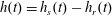 $h(t)=h_{s}(t)-h_{r}(t)$
for a parallel bearing and an external harmonic force
$h(t)=h_{s}(t)-h_{r}(t)$
for a parallel bearing and an external harmonic force
 $N(t)$
is imposed on the rotor.
$N(t)$
is imposed on the rotor.
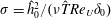
In this work we consider the fluid flow between two annular surfaces (see figure 1), where one surface, the rotor, is mounted to a rotating shaft and the other surface, the stator, is flexibly mounted to a stationary housing. The rotor experiences an external periodic axial force, due to the dynamics from the larger system that the bearing is placed within and can result in an axial rotor displacement of larger magnitude than the initial equilibrium fluid film thickness. The stator can move axially with a rigid displacement in response to the induced film dynamics from the rotor motion, where the axial displacement of the rotor and stator are each modelled as a spring–mass–damper system. The equilibrium position of the bearing refers to the case where there are no effects from an external force, the rotor has rotational motion and the hydrodynamic force due to the flow dynamics causes the rotor and stator to settle at a fixed position (equilibrium position), resulting in a film thickness
 ${\hat{h}}_{0}$
. In our analysis we consider two cases, the first where both the rotor and stator surfaces are flat, giving parallel faces, and the second where the stator surface is flat but the rotor surface has a conical shape. In the latter case the coning angle is very small to ensure that the lubrication theory developed in this work is valid.
${\hat{h}}_{0}$
. In our analysis we consider two cases, the first where both the rotor and stator surfaces are flat, giving parallel faces, and the second where the stator surface is flat but the rotor surface has a conical shape. In the latter case the coning angle is very small to ensure that the lubrication theory developed in this work is valid.
A simplified mathematical model of a gas lubricated bearing with compressible flow and a slip boundary condition imposed on the bearing faces is derived. The coaxial axisymmetric annular rotor and stator can have axial displacements, with respective heights
 ${\hat{h}}_{r}$
and
${\hat{h}}_{r}$
and
 ${\hat{h}}_{s}$
; the rotor also has rotational speed
${\hat{h}}_{s}$
; the rotor also has rotational speed
 $\hat{\unicode[STIX]{x1D6FA}}$
. A given pressure is imposed at the inner and outer radii.
$\hat{\unicode[STIX]{x1D6FA}}$
. A given pressure is imposed at the inner and outer radii.
The governing system of Navier–Stokes equations and boundary conditions for the gas flow in the bearing are expressed in dimensionless variables in terms of the exterior bearing radius
 $\hat{r}_{0}$
, equilibrium film thickness
$\hat{r}_{0}$
, equilibrium film thickness
 ${\hat{h}}_{0}$
, rotor velocity
${\hat{h}}_{0}$
, rotor velocity
 $\hat{\unicode[STIX]{x1D6FA}}\hat{r}$
, unperturbed air density
$\hat{\unicode[STIX]{x1D6FA}}\hat{r}$
, unperturbed air density
 $\hat{\unicode[STIX]{x1D70C}}_{0}$
and time scale
$\hat{\unicode[STIX]{x1D70C}}_{0}$
and time scale
 $\hat{T}$
. The dimensionless velocities are taken as
$\hat{T}$
. The dimensionless velocities are taken as
 $\hat{u} /\hat{U}$
,
$\hat{u} /\hat{U}$
,
 $\hat{v}/(\hat{\unicode[STIX]{x1D6FA}}\hat{r}_{0})$
and
$\hat{v}/(\hat{\unicode[STIX]{x1D6FA}}\hat{r}_{0})$
and
 ${\hat{w}}/({\hat{h}}_{0}\hat{T}^{-1})$
, where
${\hat{w}}/({\hat{h}}_{0}\hat{T}^{-1})$
, where
 $(\hat{u} ,\hat{v},{\hat{w}})$
are the speeds. The dimensionless radius and height are given by
$(\hat{u} ,\hat{v},{\hat{w}})$
are the speeds. The dimensionless radius and height are given by
 $r=\hat{r}/\hat{r}_{0}$
and
$r=\hat{r}/\hat{r}_{0}$
and
 $z=\hat{z}/{\hat{h}}_{0}$
, respectively, density by
$z=\hat{z}/{\hat{h}}_{0}$
, respectively, density by
 $\unicode[STIX]{x1D70C}=\hat{\unicode[STIX]{x1D70C}}/\hat{\unicode[STIX]{x1D70C}}_{0}$
and slip length by
$\unicode[STIX]{x1D70C}=\hat{\unicode[STIX]{x1D70C}}/\hat{\unicode[STIX]{x1D70C}}_{0}$
and slip length by
 $l_{s}=\hat{l_{s}}/{\hat{h}}_{0}$
. A notable feature of this work is the detailed consideration of thin film dynamics of air lubricating bearings in the slip flow regime, as characterised by values of
$l_{s}=\hat{l_{s}}/{\hat{h}}_{0}$
. A notable feature of this work is the detailed consideration of thin film dynamics of air lubricating bearings in the slip flow regime, as characterised by values of
 $10^{-3}\leqslant Kn=\tilde{\unicode[STIX]{x1D706}}/{\hat{h}}\leqslant 10^{-1}$
. For an equilibrium film thickness,
$10^{-3}\leqslant Kn=\tilde{\unicode[STIX]{x1D706}}/{\hat{h}}\leqslant 10^{-1}$
. For an equilibrium film thickness,
 ${\hat{h}}_{0}$
, of the order of
${\hat{h}}_{0}$
, of the order of
 $O(10^{-1}~\text{mm})$
and at atmospheric conditions, our characteristic film thickness in the dimensionless formulation corresponds to a value of
$O(10^{-1}~\text{mm})$
and at atmospheric conditions, our characteristic film thickness in the dimensionless formulation corresponds to a value of
 $\mathit{Kn}_{0}=\tilde{\unicode[STIX]{x1D706}}/{\hat{h}}_{0}\sim O(10^{-3})$
.
$\mathit{Kn}_{0}=\tilde{\unicode[STIX]{x1D706}}/{\hat{h}}_{0}\sim O(10^{-3})$
.

Figure 2. Cross-sectional view of a coned bearing with (a) positive and (b) negative coning angle due to over pressurisation of the bearing, with coning angle
 $\unicode[STIX]{x1D6FD}$
. The rotor–stator face clearance is now dependent on the coning angle and radial position with the minimum gap of the bearing given at the inner or outer radius.
$\unicode[STIX]{x1D6FD}$
. The rotor–stator face clearance is now dependent on the coning angle and radial position with the minimum gap of the bearing given at the inner or outer radius.
The geometry in figure 1 represents a parallel fluid lubricated bearing in the dimensionless axisymmetric coordinate system
 $(r,\unicode[STIX]{x1D703},z)$
, where the rotor experiences an imposed axial periodic force
$(r,\unicode[STIX]{x1D703},z)$
, where the rotor experiences an imposed axial periodic force
 $N(t)$
. The inner and outer radii have been rescaled as
$N(t)$
. The inner and outer radii have been rescaled as
 $a=\hat{r}_{I}/\hat{r}_{O}$
and
$a=\hat{r}_{I}/\hat{r}_{O}$
and
 $1$
, respectively, with imposed pressures
$1$
, respectively, with imposed pressures
 $p_{I}$
and
$p_{I}$
and
 $p_{O}$
. The dimensionless rotor and stator heights are denoted by
$p_{O}$
. The dimensionless rotor and stator heights are denoted by
 $h_{r}$
and
$h_{r}$
and
 $h_{s}$
and the axisymmetric rotor–stator clearance is defined by
$h_{s}$
and the axisymmetric rotor–stator clearance is defined by
 $h=h_{s}-h_{r}$
. Figure 2 gives notations for a positively coned bearing (PCB) and negatively coned bearing (NCB), where the coning angle is assumed small, i.e.
$h=h_{s}-h_{r}$
. Figure 2 gives notations for a positively coned bearing (PCB) and negatively coned bearing (NCB), where the coning angle is assumed small, i.e.
 $\sin \hat{\unicode[STIX]{x1D6FD}}=O(\unicode[STIX]{x1D6FF}_{0})$
and
$\sin \hat{\unicode[STIX]{x1D6FD}}=O(\unicode[STIX]{x1D6FF}_{0})$
and
 $\cos \hat{\unicode[STIX]{x1D6FD}}=1+O(\unicode[STIX]{x1D6FF}_{0})$
leading to the scaling
$\cos \hat{\unicode[STIX]{x1D6FD}}=1+O(\unicode[STIX]{x1D6FF}_{0})$
leading to the scaling
 $\hat{\unicode[STIX]{x1D6FD}}=\unicode[STIX]{x1D6FD}\unicode[STIX]{x1D6FF}_{0}$
with
$\hat{\unicode[STIX]{x1D6FD}}=\unicode[STIX]{x1D6FD}\unicode[STIX]{x1D6FF}_{0}$
with
 $\unicode[STIX]{x1D6FD}=O(1)$
, giving consistency with the lubrication condition. The rotor height is given as
$\unicode[STIX]{x1D6FD}=O(1)$
, giving consistency with the lubrication condition. The rotor height is given as
 $$\begin{eqnarray}\displaystyle h_{r}(r,\unicode[STIX]{x1D6FD},t)\left\{\begin{array}{@{}l@{}}h_{r}(t)-(r-a)\unicode[STIX]{x1D6FD}\quad \text{for }\unicode[STIX]{x1D6FD}>0,\quad \text{or}\\ h_{r}(t)-(r-1)\unicode[STIX]{x1D6FD}\quad \text{for }\unicode[STIX]{x1D6FD}<0,\end{array}\right. & & \displaystyle\end{eqnarray}$$
with
 $\unicode[STIX]{x2202}h_{r}/\unicode[STIX]{x2202}r=-\unicode[STIX]{x1D6FD}$
. Although it is possible to have a single formulation for positive and negative conical angles, the given definition of the rotor height in (2.1) is chosen to have the same definition of the minimum gap,
$\unicode[STIX]{x2202}h_{r}/\unicode[STIX]{x2202}r=-\unicode[STIX]{x1D6FD}$
. Although it is possible to have a single formulation for positive and negative conical angles, the given definition of the rotor height in (2.1) is chosen to have the same definition of the minimum gap,
 $g(t)$
, in both cases (see figure 2). Separation of positive and negative coning angles is due to consideration of coning arising from possible deformation of the rotor due to over pressurisation of the bearing. Therefore, internal pressurisation
$g(t)$
, in both cases (see figure 2). Separation of positive and negative coning angles is due to consideration of coning arising from possible deformation of the rotor due to over pressurisation of the bearing. Therefore, internal pressurisation
 $(p_{I}>p_{O})$
will result in a PCB and external pressurisation
$(p_{I}>p_{O})$
will result in a PCB and external pressurisation
 $(p_{I}<p_{O})$
a NCB; in both cases the pressure gradient corresponds to a diverging channel. As the bearing dynamics is investigated to examine the minimum rotor–stator clearance, the time-dependent minimum face clearance (MFC) is defined as
$(p_{I}<p_{O})$
a NCB; in both cases the pressure gradient corresponds to a diverging channel. As the bearing dynamics is investigated to examine the minimum rotor–stator clearance, the time-dependent minimum face clearance (MFC) is defined as
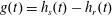 $g(t)=h_{s}(t)-h_{r}(t)$
, given at the inner radius for a PCB and outer radius for a NCB. For a parallel bearing the MFC
$g(t)=h_{s}(t)-h_{r}(t)$
, given at the inner radius for a PCB and outer radius for a NCB. For a parallel bearing the MFC
 $g(t)=h(t)$
is equal to the rotor–stator clearance. If the MFC remains positive
$g(t)=h(t)$
is equal to the rotor–stator clearance. If the MFC remains positive
 $g>0$
the bearing faces do not have contact.
$g>0$
the bearing faces do not have contact.
2.1 Air flow model
The air flow model is derived from the compressible Navier–Stokes momentum equations and the conservation of mass equation for a compressible flow in axisymmetric coordinates. The flow is assumed to be an isothermal ideal gas.
The governing system of Navier–Stokes equations and boundary conditions for the gas flow are expressed in dimensionless variables. The associated radial and azimuthal Reynolds numbers and a Reynolds number ratio
 $Re^{\ast }$
are given respectively as
$Re^{\ast }$
are given respectively as
 $$\begin{eqnarray}\displaystyle Re_{U}=\frac{\hat{U} {\hat{h}}_{0}}{\unicode[STIX]{x1D708}},\quad Re_{\unicode[STIX]{x1D6FA}}=\frac{{\hat{r}_{0}}^{2}\hat{\unicode[STIX]{x1D6FA}}}{\unicode[STIX]{x1D708}}\quad \text{and}\quad Re^{\ast }=\frac{\hat{\unicode[STIX]{x1D6FA}}\hat{r}_{0}}{\hat{U} }{\unicode[STIX]{x1D6FF}_{0}}^{-1}. & & \displaystyle\end{eqnarray}$$
The aspect ratio
 $\unicode[STIX]{x1D6FF}_{0}$
and Froude number
$\unicode[STIX]{x1D6FF}_{0}$
and Froude number
 $Fr$
are defined as
$Fr$
are defined as
 $$\begin{eqnarray}\displaystyle \unicode[STIX]{x1D6FF}_{0}=\frac{{\hat{h}}_{0}}{\hat{r}_{0}}\quad \text{and}\quad Fr=\frac{\hat{U} }{\sqrt{\tilde{g}{\hat{h}}_{0}}}, & & \displaystyle\end{eqnarray}$$
respectively, where
 $\unicode[STIX]{x1D708}=\unicode[STIX]{x1D707}/\hat{\unicode[STIX]{x1D70C}}_{0}$
is the kinematic viscosity and
$\unicode[STIX]{x1D708}=\unicode[STIX]{x1D707}/\hat{\unicode[STIX]{x1D70C}}_{0}$
is the kinematic viscosity and
 $\widetilde{g}$
denotes the acceleration due to gravity. For thin film bearings
$\widetilde{g}$
denotes the acceleration due to gravity. For thin film bearings
 $\unicode[STIX]{x1D6FF}_{0}\ll 1$
, a lubrication approximation is used and the effects of viscosity are retained at leading order with the pressure scaled as
$\unicode[STIX]{x1D6FF}_{0}\ll 1$
, a lubrication approximation is used and the effects of viscosity are retained at leading order with the pressure scaled as
 $P=\unicode[STIX]{x1D707}\hat{r}_{0}\hat{U} /{\hat{h}}_{0}^{2}$
. The Froude number
$P=\unicode[STIX]{x1D707}\hat{r}_{0}\hat{U} /{\hat{h}}_{0}^{2}$
. The Froude number
 $Fr$
parametrises the importance of the gravitational effects relative to the radial inertia, although gravity can be neglected with
$Fr$
parametrises the importance of the gravitational effects relative to the radial inertia, although gravity can be neglected with
 $Re_{U}\unicode[STIX]{x1D6FF}_{0}Fr^{-2}\ll 1$
, which is consistent with the lubrication theory provided the Froude number is
$Re_{U}\unicode[STIX]{x1D6FF}_{0}Fr^{-2}\ll 1$
, which is consistent with the lubrication theory provided the Froude number is
 $O(1)$
. Classical lubrication theory neglects inertia due to the reduced Reynolds number
$O(1)$
. Classical lubrication theory neglects inertia due to the reduced Reynolds number
 $Re_{U}\unicode[STIX]{x1D6FF}_{0}\ll 1$
, but in the case of high-speed bearing operation an additional term corresponding to the ratio of the Reynolds numbers
$Re_{U}\unicode[STIX]{x1D6FF}_{0}\ll 1$
, but in the case of high-speed bearing operation an additional term corresponding to the ratio of the Reynolds numbers
 $(Re^{\ast })^{2}$
must be considered as it is not always negligible.
$(Re^{\ast })^{2}$
must be considered as it is not always negligible.
Applying a lubrication condition, and the assumptions noted above, to the compressible Navier–Stokes momentum equations results in the leading-order momentum equations
 $$\begin{eqnarray}\displaystyle -\!\unicode[STIX]{x1D706}\unicode[STIX]{x1D70C}\frac{v^{2}}{r}=-\frac{\unicode[STIX]{x2202}p}{\unicode[STIX]{x2202}r}+\frac{\unicode[STIX]{x2202}^{2}u}{\unicode[STIX]{x2202}z^{2}},\quad 0=\frac{\unicode[STIX]{x2202}^{2}v}{\unicode[STIX]{x2202}z^{2}},\quad 0=\frac{\unicode[STIX]{x2202}p}{\unicode[STIX]{x2202}z}, & & \displaystyle\end{eqnarray}$$
with speed parameter
 $\unicode[STIX]{x1D706}=Re_{U}\unicode[STIX]{x1D6FF}_{0}(Re^{\ast })^{2}=\hat{r}_{0}{{\hat{h}}_{0}}^{2}\hat{\unicode[STIX]{x1D6FA}}^{2}/(\unicode[STIX]{x1D708}\hat{U} )$
. If
$\unicode[STIX]{x1D706}=Re_{U}\unicode[STIX]{x1D6FF}_{0}(Re^{\ast })^{2}=\hat{r}_{0}{{\hat{h}}_{0}}^{2}\hat{\unicode[STIX]{x1D6FA}}^{2}/(\unicode[STIX]{x1D708}\hat{U} )$
. If
 $\unicode[STIX]{x1D706}=0$
the standard lubrication equations for compressible flow in axisymmetric cylindrical coordinates are retained.
$\unicode[STIX]{x1D706}=0$
the standard lubrication equations for compressible flow in axisymmetric cylindrical coordinates are retained.
Similarly, the conservation of mass equation and equation of state become
 $$\begin{eqnarray}\displaystyle \frac{\unicode[STIX]{x2202}\unicode[STIX]{x1D70C}}{\unicode[STIX]{x2202}t}+\frac{1}{\unicode[STIX]{x1D70E}r}\frac{\unicode[STIX]{x2202}}{\unicode[STIX]{x2202}r}(r\unicode[STIX]{x1D70C}u)+\frac{\unicode[STIX]{x2202}}{\unicode[STIX]{x2202}z}(\unicode[STIX]{x1D70C}w)=0\quad \text{and}\quad P=K_{s}\unicode[STIX]{x1D70C}. & & \displaystyle\end{eqnarray}$$
Taking
 $\unicode[STIX]{x1D70E}={{\hat{h}}_{0}}^{2}/(\unicode[STIX]{x1D708}\hat{T}Re_{U}\unicode[STIX]{x1D6FF}_{0})$
of
$\unicode[STIX]{x1D70E}={{\hat{h}}_{0}}^{2}/(\unicode[STIX]{x1D708}\hat{T}Re_{U}\unicode[STIX]{x1D6FF}_{0})$
of
 $O(1)$
, implies in our formulation that
$O(1)$
, implies in our formulation that
 $({{\hat{h}}_{0}}^{2}/\unicode[STIX]{x1D708})/\hat{T}$
has to be of
$({{\hat{h}}_{0}}^{2}/\unicode[STIX]{x1D708})/\hat{T}$
has to be of
 $O(\unicode[STIX]{x1D6FF}_{0})$
. Therefore, the flow field time scale
$O(\unicode[STIX]{x1D6FF}_{0})$
. Therefore, the flow field time scale
 $\hat{T}$
needs to be much slower than the time scale
$\hat{T}$
needs to be much slower than the time scale
 $\unicode[STIX]{x1D70F}={{\hat{h}}_{0}}^{2}/\unicode[STIX]{x1D708}$
, the time taken for vorticity to diffuse over the film thickness
$\unicode[STIX]{x1D70F}={{\hat{h}}_{0}}^{2}/\unicode[STIX]{x1D708}$
, the time taken for vorticity to diffuse over the film thickness
 ${\hat{h}}_{0}$
. This is consistent with the quasi-static approximation of the lubrication theory where the local acceleration is of the
${\hat{h}}_{0}$
. This is consistent with the quasi-static approximation of the lubrication theory where the local acceleration is of the
 $O(Re_{U}\unicode[STIX]{x1D6FF}_{0})$
. The dimensionless ideal gas constant is given by
$O(Re_{U}\unicode[STIX]{x1D6FF}_{0})$
. The dimensionless ideal gas constant is given by
 $K_{s}=RT_{0}{\hat{h}}_{0}^{2}/\unicode[STIX]{x1D708}\hat{r}_{0}\hat{U} M$
, which relates the pressure field to the density field, where
$K_{s}=RT_{0}{\hat{h}}_{0}^{2}/\unicode[STIX]{x1D708}\hat{r}_{0}\hat{U} M$
, which relates the pressure field to the density field, where
 $R$
,
$R$
,
 $T_{0}$
and
$T_{0}$
and
 $M$
are the ideal gas constant, fluid temperature and molar mass, respectively.
$M$
are the ideal gas constant, fluid temperature and molar mass, respectively.
A first-order Navier slip model, as considered by Bailey et al. (Reference Bailey, Cliffe, Hibberd and Power2014, Reference Bailey, Cliffe, Hibberd and Power2015), is implemented, where the velocity boundary conditions comprise of tangential components where continuity of the velocity across the fluid–solid boundary is modified by a slip condition induced by the wall shear, together with a normal component of a no-flux condition. The dimensionless velocity boundary conditions to leading order are
 $$\begin{eqnarray}\displaystyle \left.\begin{array}{@{}c@{}}\displaystyle u=l_{s}\frac{\unicode[STIX]{x2202}u}{\unicode[STIX]{x2202}z},\quad v=r+l_{s}\frac{\unicode[STIX]{x2202}v}{\unicode[STIX]{x2202}z},\quad w=\frac{\unicode[STIX]{x2202}h_{r}}{\unicode[STIX]{x2202}t}-\frac{Re_{U}\unicode[STIX]{x1D6FF}_{0}}{\unicode[STIX]{x1D705}}u\unicode[STIX]{x1D6FD}\quad \text{at }z=h_{r},\\ \displaystyle u=-l_{s}\frac{\unicode[STIX]{x2202}u}{\unicode[STIX]{x2202}z},\quad v=-l_{s}\frac{\unicode[STIX]{x2202}v}{\unicode[STIX]{x2202}z},\quad w=\frac{\text{d}h_{s}}{\text{d}t}\quad \text{at }z=h_{s},\end{array}\right\} & & \displaystyle\end{eqnarray}$$
see Bailey et al. (Reference Bailey, Cliffe, Hibberd and Power2015) for full derivation. The fluid velocity components tangential to the wall in (2.6) are proportional to the wall shear stress with proportionality constant
 $l_{s}$
, a dimensionless slip length in the above expressions. The limit
$l_{s}$
, a dimensionless slip length in the above expressions. The limit
 $l_{s}=0$
corresponds to no-slip conditions and
$l_{s}=0$
corresponds to no-slip conditions and
 $l_{s}\rightarrow \infty$
to a total slip model, defined by a zero tangential wall fluid shear rate.
$l_{s}\rightarrow \infty$
to a total slip model, defined by a zero tangential wall fluid shear rate.
Within the kinetic theory of gas–solid interaction, a fluid molecule will transfer some of its tangential momentum to the solid with a collision frequency not high enough to ensure thermodynamic equilibrium, and a certain degree of tangential velocity slip occurs. Some fraction
 $f$
of the molecules colliding with the wall are diffusely reflected (the momentum accommodation coefficient), where
$f$
of the molecules colliding with the wall are diffusely reflected (the momentum accommodation coefficient), where
 $f=1$
represents diffuse reflection (gas molecule tangential momentum not conserved) and
$f=1$
represents diffuse reflection (gas molecule tangential momentum not conserved) and
 $f=0$
represents specular reflection (gas molecule tangential momentum conserved).
$f=0$
represents specular reflection (gas molecule tangential momentum conserved).
The classical theory to estimate the slip coefficient for atomically smooth walls is due to Maxwell (Reference Maxwell1879), where the slip length
 $\hat{l_{s}}$
is characterised by the tangential momentum accommodation coefficient
$\hat{l_{s}}$
is characterised by the tangential momentum accommodation coefficient
 $f$
, and the mean free molecular path
$f$
, and the mean free molecular path
 $\tilde{\unicode[STIX]{x1D706}}$
, given by the following expression:
$\tilde{\unicode[STIX]{x1D706}}$
, given by the following expression:
 $$\begin{eqnarray}\hat{l_{s}}=\unicode[STIX]{x1D6FC}_{s}\tilde{\unicode[STIX]{x1D706}}\frac{(2-f)}{f}.\end{eqnarray}$$
In terms of our dimensionless variables, the Maxwell slip length model is written as
 $$\begin{eqnarray}l_{s}=\unicode[STIX]{x1D6FC}_{s}Kn_{0}\frac{(2-f)}{f},\end{eqnarray}$$
where
 $Kn_{0}=\tilde{\unicode[STIX]{x1D706}}/{\hat{h}}_{0}$
, corresponding to the value of the Knudsen number at the equilibrium position, which is considered to be of the order of
$Kn_{0}=\tilde{\unicode[STIX]{x1D706}}/{\hat{h}}_{0}$
, corresponding to the value of the Knudsen number at the equilibrium position, which is considered to be of the order of
 $10^{-3}$
. According to the first-order Navier slip condition the value of
$10^{-3}$
. According to the first-order Navier slip condition the value of
 $\hat{l_{s}}$
, and therefore
$\hat{l_{s}}$
, and therefore
 $l_{s}$
, remains constant in the slip flow regime,
$l_{s}$
, remains constant in the slip flow regime,
 $10^{-3}\leqslant Kn\leqslant 10^{-1}$
. Therefore, the value of the dimensionless slip length,
$10^{-3}\leqslant Kn\leqslant 10^{-1}$
. Therefore, the value of the dimensionless slip length,
 $l_{s}$
, in the slip regime is determined by the value of the Knudsen number at the equilibrium position,
$l_{s}$
, in the slip regime is determined by the value of the Knudsen number at the equilibrium position,
 $Kn_{0}$
, and the accommodation coefficient
$Kn_{0}$
, and the accommodation coefficient
 $f$
.
$f$
.
Maxwell estimated the coefficient
 $\unicode[STIX]{x1D6FC}_{s}$
by considering that the incident gas molecules have the same distributions as those of the bulk gas, and obtained
$\unicode[STIX]{x1D6FC}_{s}$
by considering that the incident gas molecules have the same distributions as those of the bulk gas, and obtained
 $\unicode[STIX]{x1D6FC}_{s}=\sqrt{\unicode[STIX]{x03C0}}/2$
, which is typically approximated by unity. However, more rigorous kinetic analyses of the Boltzmann equation for planar flows (Cercignani & Daneri Reference Cercignani and Daneri1963) have shown that
$\unicode[STIX]{x1D6FC}_{s}=\sqrt{\unicode[STIX]{x03C0}}/2$
, which is typically approximated by unity. However, more rigorous kinetic analyses of the Boltzmann equation for planar flows (Cercignani & Daneri Reference Cercignani and Daneri1963) have shown that
 $\unicode[STIX]{x1D6FC}_{s}=1.1466$
, (for more details see Barber & Emerson (Reference Barber and Emerson2006)).
$\unicode[STIX]{x1D6FC}_{s}=1.1466$
, (for more details see Barber & Emerson (Reference Barber and Emerson2006)).
Following Maxwell’s original work, many other slip models have been proposed in the literature including results for atomically rough walls, for more details see the review article by Zhang et al. (Reference Zhang, Meng and Wei2012). In addition, Lilley & Sader (Reference Lilley and Sader2008) studied the Knudsen layer, which is a rarefaction effect that extends to a distance of the order of one mean free path from the solid wall, by using existing linearised Boltzmann equation solutions of Kramer’s problem for hard spherical molecules with partial thermal accommodation. Results obtained were verified by accurate direct Monte Carlo simulations of the Boltzmann equation. Lilley and Sader’s slip model written in our dimensionless form is given by:
 $$\begin{eqnarray}l_{s}=Kn_{0}\;\left(\frac{2.01}{f}-0.73-0.16f\right).\end{eqnarray}$$
The functional dependencies on the above expression was determined empirically from their results using several trial functions and nonlinear regression.
The slip condition of air flow can be determined experimentally by the use of an atomic force microscopy (AFM) cantilever. This approach is able to confine the air to very small length scales and to accurately measure very small forces due to the air flow. Honig et al. (Reference Honig, Sader, Mulvaney and Ducker2010) and Bowles & Ducker (Reference Bowles and Ducker2011) used a thermal-driven oscillation of a sphere glued to an AFM cantilever to measure the damping force versus gas film gap between the sphere and the substrate and compared the force obtained to the theoretical force obtained for a specific slip boundary condition; reported values of slip length ranged from
 $100$
to
$100$
to
 $600$
nm. Pan, Bhushan & Maali (Reference Pan, Bhushan and Maali2013) used a similar device where the sphere was forced to oscillate periodically with a prescribed amplitude where the aim was to demonstrate the slip length was independent of the oscillation amplitude of the cantilever, i.e. constant slip length. Equation (2.9) was used to determine the corresponding values of the accommodation coefficient
$600$
nm. Pan, Bhushan & Maali (Reference Pan, Bhushan and Maali2013) used a similar device where the sphere was forced to oscillate periodically with a prescribed amplitude where the aim was to demonstrate the slip length was independent of the oscillation amplitude of the cantilever, i.e. constant slip length. Equation (2.9) was used to determine the corresponding values of the accommodation coefficient
 $f$
, where imperfect accommodation was consistently observed with values within the range of
$f$
, where imperfect accommodation was consistently observed with values within the range of
 $0.4$
–
$0.4$
–
 $0.9$
. Experiments concluded that the slip length, and consequently
$0.9$
. Experiments concluded that the slip length, and consequently
 $f$
, are highly dependent on the nature of the solid surface, composition of the gas and the temperature.
$f$
, are highly dependent on the nature of the solid surface, composition of the gas and the temperature.
In addition, the slip condition for gas flows at the solid–gas interface can be significantly modified by the adsorption of the thin film into the solid. Seo & Ducker (Reference Seo and Ducker2013) reported an increase in the slip length of a monolayer of ocatadecyltrichlorosilane from
 $290$
to
$290$
to
 $590$
nm by increasing the temperature from
$590$
nm by increasing the temperature from
 $18$
to
$18$
to
 $40\,^{\circ }\text{C}$
, which was associated with an adsorption of the gas into the ocatadecyltrichlorosilane layer.
$40\,^{\circ }\text{C}$
, which was associated with an adsorption of the gas into the ocatadecyltrichlorosilane layer.
Taking into account the slip conditions (2.6), the flow velocities can be readily found from the leading-order Navier–Stokes equations (2.4). The radial, azimuthal and axial velocities are given by
 $$\begin{eqnarray}\displaystyle u & = & \displaystyle \frac{1}{2}\frac{\unicode[STIX]{x2202}p}{\unicode[STIX]{x2202}r}(z^{2}-(h_{s}+h_{r})z+h_{s}h_{r}-l_{s}h)\nonumber\\ \displaystyle & & \displaystyle -\,\frac{\unicode[STIX]{x1D706}pr}{12K_{s}(h+2ls)^{2}} ((z-h_{r})(z-h_{s})(z^{2}+(h_{r}-3h_{s})z+3h_{s}^{2}-3h_{s}h_{r}+h_{r}^{2})\nonumber\\ \displaystyle & & \displaystyle +\,l_{s}((z-h_{s})(-4(z-h_{s})^{2}+6h^{2})-h^{3})\nonumber\\ \displaystyle & & \displaystyle +\,l_{s}^{2}(6(z-h_{s})(z-h_{r})-6h)-6hl_{s}^{3} ),\end{eqnarray}$$
 $$\begin{eqnarray}\displaystyle v=-\frac{r}{(h+2l_{s})}(z-h_{s}-l_{s}), & & \displaystyle\end{eqnarray}$$
 $$\begin{eqnarray}\displaystyle w & = & \displaystyle -\frac{1}{p}\frac{\unicode[STIX]{x2202}}{\unicode[STIX]{x2202}t}((z-h_{r})p)-\frac{1}{12\unicode[STIX]{x1D70E}pr}\frac{\unicode[STIX]{x2202}}{\unicode[STIX]{x2202}r}\left(pr\frac{\unicode[STIX]{x2202}p}{\unicode[STIX]{x2202}r}(2(z-h_{r})^{3}-3(z-h_{r})^{2}h-6(z-h_{r})hl_{s})\right)\nonumber\\ \displaystyle & & \displaystyle +\,\frac{\unicode[STIX]{x1D706}}{120\unicode[STIX]{x1D70E}K_{s}pr}\frac{\unicode[STIX]{x2202}}{\unicode[STIX]{x2202}r}\left(\frac{p^{2}r^{2}}{(h+2l_{s})^{2}} (2(z-h_{r})^{5}\right.\nonumber\\ \displaystyle & & \displaystyle -\,10(z-h_{r})^{4}h+20(z-h_{r})^{3}h^{2}-15(z-h_{r})^{2}h^{3} )\nonumber\\ \displaystyle & & \displaystyle +\,10l_{s}(-(z-h_{r})^{4}+4(z-h_{r})^{3}h-3(z-h_{r})^{2}h^{2}-3(z-h_{r})h^{3})\nonumber\\ \displaystyle & & \displaystyle +\,\left.10l_{s}^{2}(2(z-h_{r})^{3}-3(z-h_{r})^{2}h-6(z-h_{r})h^{2})+10l_{s}^{3}(-6(z-h_{r})h)\right).\end{eqnarray}$$
Dependence on the coning angle appears implicitly in expressions the rotor height
 $h_{r}$
and rotor–stator clearance
$h_{r}$
and rotor–stator clearance
 $h$
.
$h$
.
Integrating the conservation of mass (2.5) between the rotor and stator, applying the Leibniz integral rule and the velocity boundary conditions (2.6), gives the modified Reynolds equation for compressible flow as
 $$\begin{eqnarray}\displaystyle & & \displaystyle \frac{\unicode[STIX]{x2202}}{\unicode[STIX]{x2202}t}(ph)-\frac{1}{12\unicode[STIX]{x1D70E}r}\frac{\unicode[STIX]{x2202}}{\unicode[STIX]{x2202}r}\left(pr\frac{\unicode[STIX]{x2202}p}{\unicode[STIX]{x2202}r}h^{2}(h+6l_{s})\right)\nonumber\\ \displaystyle & & \displaystyle \quad +\,\frac{\unicode[STIX]{x1D706}}{12K_{s}\unicode[STIX]{x1D70E}r}\frac{\unicode[STIX]{x2202}}{\unicode[STIX]{x2202}r}\left(p^{2}r^{2}\frac{h^{2}\left(\frac{3}{10}h^{3}+3h^{2}l_{s}+7h{l_{s}}^{2}+6{l_{s}}^{3}\right)}{(h+2l_{s})^{2}}\right)=0,\end{eqnarray}$$
expressing the relationship between the pressure
 $p$
and film thickness
$p$
and film thickness
 $h$
. Dependence on the coning angle is given implicitly in the rotor–stator clearance
$h$
. Dependence on the coning angle is given implicitly in the rotor–stator clearance
 $h$
. For speed parameter
$h$
. For speed parameter
 $\unicode[STIX]{x1D706}=0$
, the centrifugal effects are neglected but the rotor and stator still experience relative rotational motion due to the velocity boundary conditions.
$\unicode[STIX]{x1D706}=0$
, the centrifugal effects are neglected but the rotor and stator still experience relative rotational motion due to the velocity boundary conditions.
The pressure boundary conditions in dimensionless variables are given by
 $$\begin{eqnarray}\displaystyle p=p_{I}\quad \text{at }r=a,\quad \text{and}\quad p=p_{O}\quad \text{at }r=1. & & \displaystyle\end{eqnarray}$$
In contrast to the case of incompressible flow, an analytical solution of the above Reynolds equation (2.13) subject to the boundary condition (2.14a,b ) is not easily obtained and it is usually necessary to resort to numerical techniques.
2.2 Structural dynamics
The axial displacement of the stator and rotor are modelled using a standard spring–mass–damper model incorporating the bearing pressure variation. An external periodic force is imposed on the rotor in dimensionless form
 $N(t)=\unicode[STIX]{x1D716}\sin t$
, where
$N(t)=\unicode[STIX]{x1D716}\sin t$
, where
 $\unicode[STIX]{x1D716}$
is a measure of the amplitude of the forcing. In dimensionless variables the stator displacement equation is given by
$\unicode[STIX]{x1D716}$
is a measure of the amplitude of the forcing. In dimensionless variables the stator displacement equation is given by
 $$\begin{eqnarray}\displaystyle \frac{\text{d}^{2}h_{s}}{\text{d}t^{2}}+D_{as}\frac{\text{d}h_{s}}{\text{d}t}+K_{zs}(h_{s}-1)=\unicode[STIX]{x1D6FC}_{s}F(t), & & \displaystyle\end{eqnarray}$$
and the rotor displacement equation by
 $$\begin{eqnarray}\displaystyle \left.\begin{array}{@{}c@{}}\displaystyle \frac{\text{d}^{2}h_{r}}{\text{d}t^{2}}+D_{ar}\frac{\text{d}h_{r}}{\text{d}t}+K_{zr}h_{r}=-\unicode[STIX]{x1D6FC}_{r}(F(t)-N(t))\quad \text{for }\unicode[STIX]{x1D6FD}\geqslant 0,\\ \displaystyle \text{or }\frac{\text{d}^{2}h_{r}}{\text{d}t^{2}}+D_{ar}\frac{\text{d}h_{r}}{\text{d}t}+K_{zr}(h_{r}-(1-a)\unicode[STIX]{x1D6FD})=-\unicode[STIX]{x1D6FC}_{r}(F(t)-N(t))\quad \text{for}\quad \unicode[STIX]{x1D6FD}<0.\end{array}\right\} & & \displaystyle\end{eqnarray}$$
The axial force of the fluid on the bearing faces is given by
 $$\begin{eqnarray}\displaystyle F(t)=2\unicode[STIX]{x03C0}\int _{a}^{1}(p-p_{a})r\,\text{d}r. & & \displaystyle\end{eqnarray}$$
The dimensionless reference pressure is given by
 $p_{a}=\hat{p}_{a}/\hat{P}$
and the dimensionless force coupling parameter by
$p_{a}=\hat{p}_{a}/\hat{P}$
and the dimensionless force coupling parameter by
 $\unicode[STIX]{x1D6FC}_{i}=\unicode[STIX]{x1D708}\hat{U} {Re_{U}}^{2}\unicode[STIX]{x1D708}^{2}\hat{T}^{2}/\hat{m_{i}}{{\hat{h}}_{0}}^{4}\unicode[STIX]{x1D6FF}_{0}$
where
$\unicode[STIX]{x1D6FC}_{i}=\unicode[STIX]{x1D708}\hat{U} {Re_{U}}^{2}\unicode[STIX]{x1D708}^{2}\hat{T}^{2}/\hat{m_{i}}{{\hat{h}}_{0}}^{4}\unicode[STIX]{x1D6FF}_{0}$
where
 $i=s,r$
represents the stator and rotor, respectively, and
$i=s,r$
represents the stator and rotor, respectively, and
 $m_{i}$
is the mass of the respective plate. The dimensionless damping and effective restoring force parameters are given by
$m_{i}$
is the mass of the respective plate. The dimensionless damping and effective restoring force parameters are given by
 $D_{ai}=\hat{D}_{ai}Re_{U}\unicode[STIX]{x1D6FF}_{0}/\hat{m_{i}}\unicode[STIX]{x1D705}$
and
$D_{ai}=\hat{D}_{ai}Re_{U}\unicode[STIX]{x1D6FF}_{0}/\hat{m_{i}}\unicode[STIX]{x1D705}$
and
 $K_{zi}=\hat{K}_{zi}{Re_{U}}^{2}{\unicode[STIX]{x1D6FF}_{0}}^{2}\unicode[STIX]{x1D708}^{2}\hat{T}^{2}/\hat{m_{i}}{{\hat{h}}_{0}}^{4}$
, respectively.
$K_{zi}=\hat{K}_{zi}{Re_{U}}^{2}{\unicode[STIX]{x1D6FF}_{0}}^{2}\unicode[STIX]{x1D708}^{2}\hat{T}^{2}/\hat{m_{i}}{{\hat{h}}_{0}}^{4}$
, respectively.
3 Numerical methods
To solve the coupled model of a compressible flow bearing requires the modified Reynolds equation (2.13) to be solved simultaneously with the structural equations (2.15)–(2.16) via numerical simulation. This is in contrast to the case of incompressible flow, where an analytical solution of the corresponding Reynolds equation can be formulated.
Rewriting the above set of equations in terms of the MFC and rotor displacement enables investigations into operational conditions to maintain safe and reliable behaviour, in the presence of an external force on the rotor. The Reynolds equation is discretised in the spatial variable and approximated by a second-order central finite-difference scheme.
For a fixed bearing configuration, solutions to the coupled modified Reynolds equation (2.13) and structural equations (2.15)–(2.16) are denoted by the vector
 $\boldsymbol{g}(g(t),h_{r}(t),Z(t),Y(t),p(t))$
. Initial conditions are given by
$\boldsymbol{g}(g(t),h_{r}(t),Z(t),Y(t),p(t))$
. Initial conditions are given by
 $$\begin{eqnarray}\displaystyle \left.\begin{array}{@{}c@{}}\displaystyle g(t_{0})=g_{0},\quad h_{r}(t_{0})=h_{r0},\quad Z(t_{0})=Z_{0},\quad Y(t_{0})=Y_{0}\\ \displaystyle p(t_{0})=\frac{p_{O}(r-a)+p_{I}(1-r)}{1-a},\quad a\leqslant r\leqslant 1.\end{array}\right\} & & \displaystyle\end{eqnarray}$$
As we are looking at periodic solutions of the bearing dynamics, the above initial conditions are used to start the computational algorithm and the stroboscopic map will converge to the corresponding period solution including the pressure field, if it exists. The above initial and boundary conditions in terms of a transient formulation of the problem correspond to a stationary bearing that at
 $t_{0}$
has the rotor suddenly rotating with angular velocity
$t_{0}$
has the rotor suddenly rotating with angular velocity
 $\unicode[STIX]{x1D6FA}$
and a periodic axial force imposed. The problem is allowed to evolve in time until a periodic behaviour is attained (for more details about this transient approach see § 4).
$\unicode[STIX]{x1D6FA}$
and a periodic axial force imposed. The problem is allowed to evolve in time until a periodic behaviour is attained (for more details about this transient approach see § 4).
The system of coupled differential equations of the second order can be reduced to the following system of first-order ordinary differential equations
 $$\begin{eqnarray}\displaystyle & \displaystyle \frac{\text{d}g}{\text{d}t}=Z, & \displaystyle\end{eqnarray}$$
 $$\begin{eqnarray}\displaystyle & \displaystyle \frac{\text{d}h_{r}}{\text{d}t}=Y, & \displaystyle\end{eqnarray}$$
 $$\begin{eqnarray}\displaystyle & \displaystyle \frac{\text{d}Z}{\text{d}t}=-D_{as}Z-K_{zs}(g-1)-(D_{as}-D_{ar})Y-(K_{zs}-K_{zr})h_{r}+(\unicode[STIX]{x1D6FC}_{s}+\unicode[STIX]{x1D6FC}_{r})F-\unicode[STIX]{x1D6FC}_{r}N(t), & \displaystyle \nonumber\\ \displaystyle & & \displaystyle\end{eqnarray}$$
 $$\begin{eqnarray}\displaystyle & \displaystyle \frac{\text{d}Y}{\text{d}t}=-D_{ar}Y-K_{zr}h_{r}-\unicode[STIX]{x1D6FC}_{r}F+\unicode[STIX]{x1D6FC}_{r}N(t), & \displaystyle\end{eqnarray}$$
 $$\begin{eqnarray}\displaystyle \frac{\text{d}p_{i}}{\text{d}t} & = & \displaystyle \frac{(g+(r_{i}-a)\unicode[STIX]{x1D6FD})(g+(r_{i}-a)\unicode[STIX]{x1D6FD}+6l_{s})}{12\unicode[STIX]{x1D70E}}\left(\frac{{p_{i+1}}^{2}-{p_{i-1}}^{2}}{4r_{i}\unicode[STIX]{x1D6FF}r}+\frac{{p_{i+1}}^{2}-2{p_{i}}^{2}+{p_{i-1}}^{2}}{2\unicode[STIX]{x1D6FF}r^{2}}\right)\nonumber\\ \displaystyle & & \displaystyle -\,\frac{p_{i}Z}{(g+(r_{i}-a)\unicode[STIX]{x1D6FD})}+\frac{p_{i}(p_{i+1}-p_{i-1})}{24\unicode[STIX]{x1D70E}\unicode[STIX]{x1D6FF}r}3\unicode[STIX]{x1D6FD}(g+(r_{i}-a)\unicode[STIX]{x1D6FD}+4l_{s})\nonumber\\ \displaystyle & & \displaystyle -\,\frac{\unicode[STIX]{x1D706}}{12\unicode[STIX]{x1D70E}K_{s}}\frac{(g+(r_{i}-a)\unicode[STIX]{x1D6FD})}{(g+(r_{i}-a)\unicode[STIX]{x1D6FD}+2l_{s})^{2}}\left[\left(\frac{{p_{i+1}}^{2}{r_{i+1}}^{2}-{p_{i-1}}^{2}{r_{i-1}}^{2}}{2r_{i}\unicode[STIX]{x1D6FF}r}\right)\right.\nonumber\\ \displaystyle & & \displaystyle \times \left.\left(\frac{3}{10}(g+(r_{i}-a)\unicode[STIX]{x1D6FD})^{3}+3(g+(r_{i}-a)\unicode[STIX]{x1D6FD})^{2}l_{s}+7(g+(r_{i}-a)\unicode[STIX]{x1D6FD}){l_{s}}^{2}+6{l_{s}}^{3}\right)\right]\nonumber\\ \displaystyle & & \displaystyle -\,\frac{\unicode[STIX]{x1D706}}{12\unicode[STIX]{x1D70E}K_{s}}\frac{{p_{i}}^{2}r_{i}\unicode[STIX]{x1D6FD}}{(g+(r_{i}-a)\unicode[STIX]{x1D6FD}+2l_{s})^{3}}\left(\frac{9}{10}(g+(r_{i}-a)\unicode[STIX]{x1D6FD})^{4}+9(g+(r_{i}-a)\unicode[STIX]{x1D6FD})^{3}l_{s}\right.\nonumber\\ \displaystyle & & \displaystyle +\,\left.31(g+(r_{i}-a)\unicode[STIX]{x1D6FD})^{2}{l_{s}}^{2}+42(g+(r_{i}-a)\unicode[STIX]{x1D6FD}){l_{s}}^{3}+24{l_{s}}^{4}\right).\end{eqnarray}$$
The right-hand side of the last expression in (3.6) corresponds to the finite-difference (FD) approximation of the spatial derivatives of the Reynolds equation (2.13), with
 $i=2:(M-1)$
the FD collocation points and
$i=2:(M-1)$
the FD collocation points and
 $M$
the total number of discretisation points. From the numerical point of view, this represents the main contribution of the work where the first-order differential forms of (2.15)–(2.16) are coupled with the FD approximation of the spatial derivatives of the Reynolds equation to form an extended system of first-order ordinary differential equations to be solved with the stroboscopic map algorithm. The boundary conditions for the pressure give
$M$
the total number of discretisation points. From the numerical point of view, this represents the main contribution of the work where the first-order differential forms of (2.15)–(2.16) are coupled with the FD approximation of the spatial derivatives of the Reynolds equation to form an extended system of first-order ordinary differential equations to be solved with the stroboscopic map algorithm. The boundary conditions for the pressure give
 $p_{1}=p_{I}$
and
$p_{1}=p_{I}$
and
 $p_{M}=p_{O}$
. By numerical quadrature, the force of the fluid on the faces given by (2.17) can be approximated by
$p_{M}=p_{O}$
. By numerical quadrature, the force of the fluid on the faces given by (2.17) can be approximated by
 $F=2\unicode[STIX]{x03C0}(\sum _{i=1}^{M}w_{i}(p_{i}-p_{a})r_{i})$
, where
$F=2\unicode[STIX]{x03C0}(\sum _{i=1}^{M}w_{i}(p_{i}-p_{a})r_{i})$
, where
 $w_{i}$
is a weighting function.
$w_{i}$
is a weighting function.
As the rotor experiences a periodic force with period
 $T$
, it is expected the system of (3.6)/(A 6) will have periodic solutions. Therefore a
$T$
, it is expected the system of (3.6)/(A 6) will have periodic solutions. Therefore a
 ${\Re ^{2}\rightarrow \Re }^{2}$
map is formulated, advancing an initial condition
${\Re ^{2}\rightarrow \Re }^{2}$
map is formulated, advancing an initial condition
 $\boldsymbol{g}_{0}$
at time
$\boldsymbol{g}_{0}$
at time
 $t_{0}$
by a time
$t_{0}$
by a time
 $T$
, defining a stroboscopic map
$T$
, defining a stroboscopic map
 $\unicode[STIX]{x1D719}(T;\boldsymbol{g}_{0},t_{0})$
. This map integrates the system of (3.6)/(A 6) forward through one period of the forcing. Periodic solutions are identified via the fixed points of the stroboscopic map
$\unicode[STIX]{x1D719}(T;\boldsymbol{g}_{0},t_{0})$
. This map integrates the system of (3.6)/(A 6) forward through one period of the forcing. Periodic solutions are identified via the fixed points of the stroboscopic map
 $\boldsymbol{g}(t)=\boldsymbol{g}(t+T)$
and found iteratively, corresponding to the condition
$\boldsymbol{g}(t)=\boldsymbol{g}(t+T)$
and found iteratively, corresponding to the condition
 $$\begin{eqnarray}\displaystyle \boldsymbol{g}(T)-\boldsymbol{g}(t_{0})=\unicode[STIX]{x1D753}(T;\boldsymbol{g}_{0},t_{0})-\boldsymbol{g}_{0}=\boldsymbol{G}(\unicode[STIX]{x1D753}(T;\boldsymbol{g}_{0},t_{t}),\boldsymbol{g}_{0})=0, & & \displaystyle\end{eqnarray}$$
giving periodic solutions
 $\boldsymbol{g}(g(t),h_{r}(t),Z(t),Y(t),p_{i}(t))$
. A similar approach was used by Bailey et al. (Reference Bailey, Cliffe, Hibberd and Power2015), where the pressure field was given by its analytical solution instead of its finite-difference numerical approximation as required in the present case.
$\boldsymbol{g}(g(t),h_{r}(t),Z(t),Y(t),p_{i}(t))$
. A similar approach was used by Bailey et al. (Reference Bailey, Cliffe, Hibberd and Power2015), where the pressure field was given by its analytical solution instead of its finite-difference numerical approximation as required in the present case.
An iterative Newton’s method is used to find solutions numerically, given an initial guess value
 $\tilde{\boldsymbol{g}}_{0}$
. Successively improved iterates of the initial guess
$\tilde{\boldsymbol{g}}_{0}$
. Successively improved iterates of the initial guess
 $\boldsymbol{g}_{0}$
are computed by the numerical iterative scheme
$\boldsymbol{g}_{0}$
are computed by the numerical iterative scheme
 $$\begin{eqnarray}\displaystyle \boldsymbol{g}_{0_{n+1}}=\tilde{\boldsymbol{g}}_{0_{n}}-\unicode[STIX]{x1D645}(T)^{-1}(\boldsymbol{g}(T)-\tilde{\boldsymbol{g}}_{0_{n}}), & & \displaystyle\end{eqnarray}$$
with the Jacobian matrix
 $$\begin{eqnarray}\displaystyle \unicode[STIX]{x1D645}(T) & = & \displaystyle \frac{\unicode[STIX]{x2202}\boldsymbol{G}(\unicode[STIX]{x1D753},\boldsymbol{g}_{0})}{\unicode[STIX]{x2202}\boldsymbol{g}_{0}}\nonumber\\ \displaystyle & = & \displaystyle \left[\begin{array}{@{}ccccc@{}}\displaystyle \frac{\unicode[STIX]{x2202}g(T)}{\unicode[STIX]{x2202}g_{0}}-1 & \displaystyle \frac{\unicode[STIX]{x2202}g(T)}{\unicode[STIX]{x2202}h_{r0}} & \displaystyle \frac{\unicode[STIX]{x2202}g(T)}{\unicode[STIX]{x2202}z_{0}} & \displaystyle \frac{\unicode[STIX]{x2202}g(T)}{\unicode[STIX]{x2202}Y_{0}} & \displaystyle \frac{\unicode[STIX]{x2202}g(T)}{\unicode[STIX]{x2202}p_{i0}}\\ \displaystyle \frac{\unicode[STIX]{x2202}h_{r}(T)}{\unicode[STIX]{x2202}g_{0}} & \displaystyle \frac{\unicode[STIX]{x2202}h_{r}(T)}{\unicode[STIX]{x2202}h_{r0}}-1 & \displaystyle \frac{\unicode[STIX]{x2202}h_{r}(T)}{\unicode[STIX]{x2202}z_{0}} & \displaystyle \frac{\unicode[STIX]{x2202}h_{r}(T)}{\unicode[STIX]{x2202}Y_{0}} & \displaystyle \frac{\unicode[STIX]{x2202}h_{r}(T)}{\unicode[STIX]{x2202}p_{i0}}\\ \displaystyle \frac{\unicode[STIX]{x2202}Z(T)}{\unicode[STIX]{x2202}g_{0}} & \displaystyle \frac{\unicode[STIX]{x2202}Z(T)}{\unicode[STIX]{x2202}h_{r0}} & \displaystyle \frac{\unicode[STIX]{x2202}Z(T)}{\unicode[STIX]{x2202}z_{0}}-1 & \displaystyle \frac{\unicode[STIX]{x2202}Z(T)}{\unicode[STIX]{x2202}Y_{0}} & \displaystyle \frac{\unicode[STIX]{x2202}Z(T)}{\unicode[STIX]{x2202}p_{i0}}\\ \displaystyle \frac{\unicode[STIX]{x2202}Y(T)}{\unicode[STIX]{x2202}g_{0}} & \displaystyle \frac{\unicode[STIX]{x2202}Y(T)}{\unicode[STIX]{x2202}h_{r0}} & \displaystyle \frac{\unicode[STIX]{x2202}Y(T)}{\unicode[STIX]{x2202}z_{0}} & \displaystyle \frac{\unicode[STIX]{x2202}Y(T)}{\unicode[STIX]{x2202}Y_{0}}-1 & \displaystyle \frac{\unicode[STIX]{x2202}Y(T)}{\unicode[STIX]{x2202}p_{i0}}\\ \displaystyle \frac{\unicode[STIX]{x2202}p_{i}(T)}{\unicode[STIX]{x2202}g_{0}} & \displaystyle \frac{\unicode[STIX]{x2202}p_{i}(T)}{\unicode[STIX]{x2202}h_{r0}} & \displaystyle \frac{\unicode[STIX]{x2202}p_{i}(T)}{\unicode[STIX]{x2202}z_{0}} & \displaystyle \frac{\unicode[STIX]{x2202}p_{i}(T)}{\unicode[STIX]{x2202}Y_{0}} & \displaystyle \frac{\unicode[STIX]{x2202}p_{i}(T)}{\unicode[STIX]{x2202}p_{i0}}-I_{i}\end{array}\right].\hspace{10.0pt}\end{eqnarray}$$
To find the elements of the Jacobian matrix
 $\unicode[STIX]{x1D645}(T)$
, an auxiliary system of first-order differential equations is defined and given in the appendix, § A.1, system (A 1) with the corresponding initial conditions of the system given by (A 2).
$\unicode[STIX]{x1D645}(T)$
, an auxiliary system of first-order differential equations is defined and given in the appendix, § A.1, system (A 1) with the corresponding initial conditions of the system given by (A 2).
Thus for any given initial condition, a solution of the system of (3.6)/(A 6) and (A 1)/(A 7) for
 $t_{0}\leqslant t\leqslant T$
can be found using the Matlab ode15s routine for the solution of a system of first-order ordinary differential equations. The procedure is repeated recursively, each time using an improved initial guess
$t_{0}\leqslant t\leqslant T$
can be found using the Matlab ode15s routine for the solution of a system of first-order ordinary differential equations. The procedure is repeated recursively, each time using an improved initial guess
 $\boldsymbol{g}_{0}$
for the system of (3.6)/(A 6), until a prescribed tolerance,
$\boldsymbol{g}_{0}$
for the system of (3.6)/(A 6), until a prescribed tolerance,
 $\text{tol}$
, is achieved, i.e.
$\text{tol}$
, is achieved, i.e.
 $|\boldsymbol{g}(T)-\boldsymbol{g}_{0}(t_{0})|\leqslant \text{tol}$
resulting in a periodic solution.
$|\boldsymbol{g}(T)-\boldsymbol{g}_{0}(t_{0})|\leqslant \text{tol}$
resulting in a periodic solution.
To find a periodic solution for increasing amplitude of rotor forcing
 $\unicode[STIX]{x1D716}+\unicode[STIX]{x0394}\unicode[STIX]{x1D716}$
, a new initial condition is needed. Therefore an Euler scheme (parameter continuation) is formulated for which the solution is now defined with the amplitude of rotor forcing as a variable parameter;
$\unicode[STIX]{x1D716}+\unicode[STIX]{x0394}\unicode[STIX]{x1D716}$
, a new initial condition is needed. Therefore an Euler scheme (parameter continuation) is formulated for which the solution is now defined with the amplitude of rotor forcing as a variable parameter;
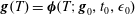 $\boldsymbol{g}(T)=\unicode[STIX]{x1D753}(T;\boldsymbol{g}_{0},t_{0},\unicode[STIX]{x1D716}_{0})$
. To compute a new initial condition
$\boldsymbol{g}(T)=\unicode[STIX]{x1D753}(T;\boldsymbol{g}_{0},t_{0},\unicode[STIX]{x1D716}_{0})$
. To compute a new initial condition
 $\boldsymbol{g}_{0}$
for
$\boldsymbol{g}_{0}$
for
 $\unicode[STIX]{x1D716}+\unicode[STIX]{x0394}\unicode[STIX]{x1D716}$
, the derivative
$\unicode[STIX]{x1D716}+\unicode[STIX]{x0394}\unicode[STIX]{x1D716}$
, the derivative
 $\boldsymbol{G}(\unicode[STIX]{x1D753}(T;\boldsymbol{g}_{0},t_{0}),\boldsymbol{g}_{0})=\unicode[STIX]{x1D753}(T;\boldsymbol{g}_{0},t_{0})-\boldsymbol{g}_{0}=0$
is taken with respect to the amplitude of rotor forcing
$\boldsymbol{G}(\unicode[STIX]{x1D753}(T;\boldsymbol{g}_{0},t_{0}),\boldsymbol{g}_{0})=\unicode[STIX]{x1D753}(T;\boldsymbol{g}_{0},t_{0})-\boldsymbol{g}_{0}=0$
is taken with respect to the amplitude of rotor forcing
 $\unicode[STIX]{x1D716}$
:
$\unicode[STIX]{x1D716}$
:
 $$\begin{eqnarray}\displaystyle \frac{\unicode[STIX]{x2202}\boldsymbol{G}}{\unicode[STIX]{x2202}\boldsymbol{g}_{0}}\frac{\unicode[STIX]{x2202}\boldsymbol{g}_{0}}{\unicode[STIX]{x2202}\unicode[STIX]{x1D716}}+\frac{\unicode[STIX]{x2202}\unicode[STIX]{x1D753}}{\unicode[STIX]{x2202}\unicode[STIX]{x1D716}}=\unicode[STIX]{x1D645}(T)\frac{\unicode[STIX]{x2202}\boldsymbol{g}_{0}}{\unicode[STIX]{x2202}\unicode[STIX]{x1D716}}+\frac{\unicode[STIX]{x2202}\boldsymbol{g}(T)}{\unicode[STIX]{x2202}\unicode[STIX]{x1D716}}=0. & & \displaystyle\end{eqnarray}$$
An Euler predictor step is then executed
 $$\begin{eqnarray}\displaystyle \boldsymbol{g}_{0}(\unicode[STIX]{x1D716}+\unicode[STIX]{x0394}\unicode[STIX]{x1D716})=\boldsymbol{g}_{0}(\unicode[STIX]{x1D716})+\frac{\unicode[STIX]{x2202}\boldsymbol{g}_{0}}{\unicode[STIX]{x2202}\unicode[STIX]{x1D716}}\unicode[STIX]{x0394}\unicode[STIX]{x1D716}=\boldsymbol{g}_{0}(\unicode[STIX]{x1D716})-\unicode[STIX]{x1D645}(T)^{-1}\frac{\unicode[STIX]{x2202}\boldsymbol{g}(T)}{\unicode[STIX]{x2202}\unicode[STIX]{x1D716}}\unicode[STIX]{x0394}\unicode[STIX]{x1D716}. & & \displaystyle\end{eqnarray}$$
The inverse of the Jacobian matrix is as found previously, with the value of
 $\unicode[STIX]{x1D716}$
corresponding to the periodic solution obtained.
$\unicode[STIX]{x1D716}$
corresponding to the periodic solution obtained.
To achieve the values of
 $\unicode[STIX]{x2202}\boldsymbol{g}(T)/\unicode[STIX]{x2202}\unicode[STIX]{x1D716}$
, an auxiliary system of first-order differential equations is defined as given in the appendix, § A.1, system (A 3), with the corresponding initial conditions (A 4). This additional system of equations is coupled to the previous augmented system of equations and solved using the same Matlab routine.
$\unicode[STIX]{x2202}\boldsymbol{g}(T)/\unicode[STIX]{x2202}\unicode[STIX]{x1D716}$
, an auxiliary system of first-order differential equations is defined as given in the appendix, § A.1, system (A 3), with the corresponding initial conditions (A 4). This additional system of equations is coupled to the previous augmented system of equations and solved using the same Matlab routine.
The above Newton procedure is iterated until convergence is achieved and a periodic solution for
 $\unicode[STIX]{x1D716}+\unicode[STIX]{x0394}\unicode[STIX]{x1D716}$
is found. To ensure convergence, an initial value of
$\unicode[STIX]{x1D716}+\unicode[STIX]{x0394}\unicode[STIX]{x1D716}$
is found. To ensure convergence, an initial value of
 $\unicode[STIX]{x0394}\unicode[STIX]{x1D716}$
was successively halved until a converged solution was found.
$\unicode[STIX]{x0394}\unicode[STIX]{x1D716}$
was successively halved until a converged solution was found.
A major advantage of the above Euler formulation is that it can be directly extended to compute the threshold values of the amplitude of rotor forcing
 $\unicode[STIX]{x1D716}$
corresponding to any specified minimum value of the MFC over a period cycle,
$\unicode[STIX]{x1D716}$
corresponding to any specified minimum value of the MFC over a period cycle,
 $g_{min}$
, with the limiting case of contact,
$g_{min}$
, with the limiting case of contact,
 $g_{min}=0$
. This type of analysis is of significant importance in bearing design in order to determine acceptable maximum force and amplitude of external disturbances when defining an operational minimum gap. It is important to mention that the prediction of contact is only speculative since in such a limit only molecular dynamics is representative of the gas flow before contact; however, this type of analysis can be used to indicate possible contact.
$g_{min}=0$
. This type of analysis is of significant importance in bearing design in order to determine acceptable maximum force and amplitude of external disturbances when defining an operational minimum gap. It is important to mention that the prediction of contact is only speculative since in such a limit only molecular dynamics is representative of the gas flow before contact; however, this type of analysis can be used to indicate possible contact.
In the case of a specified minimum value of the face clearance over the period
 $g_{min}$
, it is necessary to consider the amplitude of the rotor forcing
$g_{min}$
, it is necessary to consider the amplitude of the rotor forcing
 $\unicode[STIX]{x1D716}$
as a new dependent variable in the Newton scheme, giving the unknown vector to be determined as
$\unicode[STIX]{x1D716}$
as a new dependent variable in the Newton scheme, giving the unknown vector to be determined as
 $\boldsymbol{g}=(g(T),z(T),\unicode[STIX]{x1D716})$
with initial guess value
$\boldsymbol{g}=(g(T),z(T),\unicode[STIX]{x1D716})$
with initial guess value
 $\boldsymbol{g}_{0}=(g_{0},z_{0},\unicode[STIX]{x1D716}_{0})$
. A corresponding additional constraint equation
$\boldsymbol{g}_{0}=(g_{0},z_{0},\unicode[STIX]{x1D716}_{0})$
. A corresponding additional constraint equation
 $g_{min}-g^{\ast }=0$
is added, with
$g_{min}-g^{\ast }=0$
is added, with
 $g^{\ast }$
as the prescribed
$g^{\ast }$
as the prescribed
 $g_{min}$
and the corresponding Jacobian matrix given by
$g_{min}$
and the corresponding Jacobian matrix given by
 $$\begin{eqnarray}\displaystyle \unicode[STIX]{x1D645}=\left[\begin{array}{@{}cccccc@{}}\displaystyle \frac{\unicode[STIX]{x2202}g(T)}{\unicode[STIX]{x2202}g_{0}}-1 & \displaystyle \frac{\unicode[STIX]{x2202}g(T)}{\unicode[STIX]{x2202}h_{r0}} & \displaystyle \frac{\unicode[STIX]{x2202}g(T)}{\unicode[STIX]{x2202}z_{0}} & \displaystyle \frac{\unicode[STIX]{x2202}g(T)}{\unicode[STIX]{x2202}Y_{0}} & \displaystyle \frac{\unicode[STIX]{x2202}g(T)}{\unicode[STIX]{x2202}p_{i0}} & \displaystyle \frac{\unicode[STIX]{x2202}g(T)}{\unicode[STIX]{x2202}\unicode[STIX]{x1D716}_{0}}\\ \displaystyle \frac{\unicode[STIX]{x2202}h_{r}(T)}{\unicode[STIX]{x2202}g_{0}} & \displaystyle \frac{\unicode[STIX]{x2202}h_{r}(T)}{\unicode[STIX]{x2202}h_{r0}}-1 & \displaystyle \frac{\unicode[STIX]{x2202}h_{r}(T)}{\unicode[STIX]{x2202}z_{0}} & \displaystyle \frac{\unicode[STIX]{x2202}h_{r}(T)}{\unicode[STIX]{x2202}Y_{0}} & \displaystyle \frac{\unicode[STIX]{x2202}h_{r}(T)}{\unicode[STIX]{x2202}p_{i0}} & \displaystyle \frac{\unicode[STIX]{x2202}h_{r}(T)}{\unicode[STIX]{x2202}\unicode[STIX]{x1D716}_{0}}\\ \displaystyle \frac{\unicode[STIX]{x2202}Z(T)}{\unicode[STIX]{x2202}g_{0}} & \displaystyle \frac{\unicode[STIX]{x2202}Z(T)}{\unicode[STIX]{x2202}h_{r0}} & \displaystyle \frac{\unicode[STIX]{x2202}Z(T)}{\unicode[STIX]{x2202}z_{0}}-1 & \displaystyle \frac{\unicode[STIX]{x2202}Z(T)}{\unicode[STIX]{x2202}Y_{0}} & \displaystyle \frac{\unicode[STIX]{x2202}Z(T)}{\unicode[STIX]{x2202}p_{i0}} & \displaystyle \frac{\unicode[STIX]{x2202}Z(T)}{\unicode[STIX]{x2202}\unicode[STIX]{x1D716}_{0}}\\ \displaystyle \frac{\unicode[STIX]{x2202}Y(T)}{\unicode[STIX]{x2202}g_{0}} & \displaystyle \frac{\unicode[STIX]{x2202}Y(T)}{\unicode[STIX]{x2202}h_{r0}} & \displaystyle \frac{\unicode[STIX]{x2202}Y(T)}{\unicode[STIX]{x2202}z_{0}} & \displaystyle \frac{\unicode[STIX]{x2202}Y(T)}{\unicode[STIX]{x2202}Y_{0}}-1 & \displaystyle \frac{\unicode[STIX]{x2202}Y(T)}{\unicode[STIX]{x2202}p_{i0}} & \displaystyle \frac{\unicode[STIX]{x2202}Y(T)}{\unicode[STIX]{x2202}\unicode[STIX]{x1D716}_{0}}\\ \displaystyle \frac{\unicode[STIX]{x2202}p_{i}(T)}{\unicode[STIX]{x2202}g_{0}} & \displaystyle \frac{\unicode[STIX]{x2202}p_{i}(T)}{\unicode[STIX]{x2202}h_{r0}} & \displaystyle \frac{\unicode[STIX]{x2202}p_{i}(T)}{\unicode[STIX]{x2202}z_{0}} & \displaystyle \frac{\unicode[STIX]{x2202}p_{i}(T)}{\unicode[STIX]{x2202}Y_{0}} & \displaystyle \frac{\unicode[STIX]{x2202}p_{i}(T)}{\unicode[STIX]{x2202}p_{i0}}-I_{i} & \displaystyle \frac{\unicode[STIX]{x2202}p_{i}(T)}{\unicode[STIX]{x2202}\unicode[STIX]{x1D716}_{0}}\\ \displaystyle \frac{\unicode[STIX]{x2202}g_{min}}{\unicode[STIX]{x2202}g_{0}} & \displaystyle \frac{\unicode[STIX]{x2202}g_{min}}{\unicode[STIX]{x2202}h_{r0}} & \displaystyle \frac{\unicode[STIX]{x2202}g_{min}}{\unicode[STIX]{x2202}z_{0}} & \displaystyle \frac{\unicode[STIX]{x2202}g_{min}}{\unicode[STIX]{x2202}Y_{0}} & \displaystyle \frac{\unicode[STIX]{x2202}g_{min}}{\unicode[STIX]{x2202}p_{i0}} & \displaystyle \frac{\unicode[STIX]{x2202}g_{min}}{\unicode[STIX]{x2202}\unicode[STIX]{x1D716}_{0}}\end{array}\right]. & & \displaystyle \nonumber\\ \displaystyle & & \displaystyle\end{eqnarray}$$
The extra terms in the Jacobian matrix (3.12) compared to (3.9), i.e. the last column and row in (3.12), are obtained from the augmented system of first-order differential equations (A 1) and (A 3). The values in the last row are determined at the time when
 $g_{min}$
is achieved. The threshold value of the amplitude of rotor forcing, at the specified
$g_{min}$
is achieved. The threshold value of the amplitude of rotor forcing, at the specified
 $g_{min}$
, can be successively decreased to contact,
$g_{min}$
, can be successively decreased to contact,
 $g^{\ast }=0$
. Continuation is used for a new value of the specified
$g^{\ast }=0$
. Continuation is used for a new value of the specified
 $g^{\ast }$
to give
$g^{\ast }$
to give
 $$\begin{eqnarray}\displaystyle \boldsymbol{g}_{0}(g^{\ast }+\unicode[STIX]{x0394}g^{\ast })=\boldsymbol{g}_{0}(g^{\ast })-\unicode[STIX]{x1D645}^{-1}\frac{\unicode[STIX]{x2202}\boldsymbol{g}}{\unicode[STIX]{x2202}g^{\ast }}\unicode[STIX]{x0394}g^{\ast }, & & \displaystyle\end{eqnarray}$$
with
 $\unicode[STIX]{x0394}g^{\ast }<0$
and using Jacobian (3.12). A first-order forward finite-difference approximation is used to numerically evaluate the value of
$\unicode[STIX]{x0394}g^{\ast }<0$
and using Jacobian (3.12). A first-order forward finite-difference approximation is used to numerically evaluate the value of
 $\unicode[STIX]{x2202}\boldsymbol{g}/\unicode[STIX]{x2202}g^{\ast }$
in terms of the obtained solution
$\unicode[STIX]{x2202}\boldsymbol{g}/\unicode[STIX]{x2202}g^{\ast }$
in terms of the obtained solution
 $\boldsymbol{g}(g^{\ast })$
and a new auxiliary solution
$\boldsymbol{g}(g^{\ast })$
and a new auxiliary solution
 $\boldsymbol{g}(\tilde{g}^{\ast })$
, corresponding to a specified
$\boldsymbol{g}(\tilde{g}^{\ast })$
, corresponding to a specified
 $g_{min}$
,
$g_{min}$
,
 $\tilde{g}^{\ast }=g^{\ast }+\unicode[STIX]{x1D702}\unicode[STIX]{x0394}g^{\ast }$
, with
$\tilde{g}^{\ast }=g^{\ast }+\unicode[STIX]{x1D702}\unicode[STIX]{x0394}g^{\ast }$
, with
 $\unicode[STIX]{x1D702}\ll 1$
. This results in a new initial condition being defined and a periodic solution for a decreased
$\unicode[STIX]{x1D702}\ll 1$
. This results in a new initial condition being defined and a periodic solution for a decreased
 $g_{min}$
value
$g_{min}$
value
 $g^{\ast }+\unicode[STIX]{x0394}g^{\ast }$
can be computed.
$g^{\ast }+\unicode[STIX]{x0394}g^{\ast }$
can be computed.
4 Results
4.1 Comparison between compressible and incompressible models
The numerical results obtained via the stroboscopic map numerical algorithm for the fluid structure interaction of a gas lubricating bearing (compressible flow) are compared to those obtained for a liquid bearing (incompressible flow), previously considered by Bailey et al. (Reference Bailey, Cliffe, Hibberd and Power2014), including the limit when bearing configurations are such that a compressible flow can be dynamically represented as an incompressible flow. This last case is used as confirmation of the modified stroboscopic map algorithm proposed in this work.
In Bailey et al. (Reference Bailey, Cliffe, Hibberd and Power2014, Reference Bailey, Cliffe, Hibberd and Power2015), for incompressible flow bearings, a prescribed periodic harmonic displacement of the rotor is considered instead of an external harmonic force imposed upon it. Therefore, the mathematical model for a fluid lubricated bearing with incompressible flow in the references needs to be reformulated and the stroboscopic map solver described previously is adapted, in order to consider the effect of an external periodic harmonic force imposed on the rotor in both cases (compressible and incompressible). Using the scalings and assumptions, as for the compressible case in § 2, a governing equation for bearing flow is readily obtained from the leading-order thin film approximation of the Navier–Stokes continuity equation, where formally terms of
 $O(\unicode[STIX]{x1D6FF}_{0})$
are neglected. A parallel faced bearing is considered and the rotor and stator are considered to have identical structural parameters (
$O(\unicode[STIX]{x1D6FF}_{0})$
are neglected. A parallel faced bearing is considered and the rotor and stator are considered to have identical structural parameters (
 $D_{as}=D_{ar}=D_{a}$
and
$D_{as}=D_{ar}=D_{a}$
and
 $K_{zs}=K_{zr}=K_{z}$
). Thus, the modified Reynolds equation for incompressible flow bearing is given as
$K_{zs}=K_{zr}=K_{z}$
). Thus, the modified Reynolds equation for incompressible flow bearing is given as
 $$\begin{eqnarray}\displaystyle \frac{\text{d}g}{\text{d}t}-\frac{g^{2}(g+6l_{s})}{12\unicode[STIX]{x1D70E}r}\frac{\unicode[STIX]{x2202}}{\unicode[STIX]{x2202}r}\left(r\frac{\unicode[STIX]{x2202}p}{\unicode[STIX]{x2202}r}\right)+\frac{\unicode[STIX]{x1D706}}{40\unicode[STIX]{x1D70E}r}\frac{\left(g^{5}+10g^{4}l_{s}+\displaystyle \frac{70}{3}g^{3}l_{s}^{2}+20g^{2}l_{s}^{3}\right)}{(g+2l_{s})^{2}}\frac{\unicode[STIX]{x2202}}{\unicode[STIX]{x2202}r}(r^{2})=0, & & \displaystyle \nonumber\\ \displaystyle & & \displaystyle\end{eqnarray}$$
which gives the relationship between the internal bearing flow pressure
 $p$
and MFC
$p$
and MFC
 $g$
.
$g$
.
Solving the coupled model of a bearing with incompressible flow requires the modified Reynolds equation (4.1) to be solved simultaneously with the structural (2.15)/(2.16). Integrating the modified Reynolds equation (4.1) and imposing the pressure boundary conditions (2.14a,b ) gives an explicit analytical expression for the pressure. Integrating the pressure field using integral (2.17) gives the force on the bearing faces, and substituting into the structural (2.15)/(2.16) gives a system of nonlinear second-order non-autonomous ordinary differential equations for the face clearance and rotor height, of the form
 $$\begin{eqnarray}\displaystyle \left.\begin{array}{@{}c@{}}\displaystyle \frac{\text{d}^{2}g}{\text{d}t^{2}}+(D_{a}-2\unicode[STIX]{x1D6FC}B(g,ls))\frac{\text{d}g}{\text{d}t}+K_{z}(g-1)-2\unicode[STIX]{x1D6FC}A(g,\unicode[STIX]{x1D706},ls)+\unicode[STIX]{x1D6FC}N(t)=0,\\ \displaystyle \frac{\text{d}^{2}h_{r}}{\text{d}t^{2}}+D_{a}\frac{\text{d}h_{r}}{\text{d}t}+K_{z}h_{r}+\unicode[STIX]{x1D6FC}\left(A(g,\unicode[STIX]{x1D706},ls)+B(g,ls)\frac{\text{d}g}{\text{d}t}\right)-\unicode[STIX]{x1D6FC}N(t)=0.\end{array}\right\} & & \displaystyle\end{eqnarray}$$
Expressions for
 $A(g,\unicode[STIX]{x1D706},l_{s})$
and
$A(g,\unicode[STIX]{x1D706},l_{s})$
and
 $B(g,l_{s})$
are given by
$B(g,l_{s})$
are given by
 $$\begin{eqnarray}\displaystyle A(g,\unicode[STIX]{x1D706},l_{s}) & = & \displaystyle \unicode[STIX]{x03C0}\left((1-a^{2})(p_{I}-p_{a})+(p_{O}-p_{I})\left(\frac{(1-a^{2})}{2\ln a}+1\right)\right.\nonumber\\ \displaystyle & & \displaystyle -\,\left.\unicode[STIX]{x1D706}\frac{g^{3}+10g^{2}l_{s}+\displaystyle {\textstyle \frac{70}{3}}g{l_{s}}^{2}+20{l_{s}}^{3}}{4(g+6l_{s})(g+2l_{s})^{2}}\left(1-a^{4}+\frac{(1-a^{2})^{2}}{\ln a}\right)\right),\end{eqnarray}$$
 $$\begin{eqnarray}\displaystyle B(g,l_{s}) & = & \displaystyle -\frac{\unicode[STIX]{x03C0}\unicode[STIX]{x1D70E}}{8g^{2}(g+6l_{s})}\left(1-a^{4}+\frac{(1-a^{2})^{2}}{\ln a}\right).\end{eqnarray}$$
Equation (4.4) identifies that for a steady bearing with negligible inertial effects,
 $\unicode[STIX]{x1D706}=0$
, the pressure field and force on the stator is independent of the slip length. For more details on the above analytical integration of the incompressible Reynolds equation see Bailey et al. (Reference Bailey, Cliffe, Hibberd and Power2015). In terms of the numerical scheme, this is the main difference between the cases of incompressible and compressible flows, where the lack of an analytical solution of the nonlinear Reynolds equation for compressible flows is replaced by a finite-difference approximation.
$\unicode[STIX]{x1D706}=0$
, the pressure field and force on the stator is independent of the slip length. For more details on the above analytical integration of the incompressible Reynolds equation see Bailey et al. (Reference Bailey, Cliffe, Hibberd and Power2015). In terms of the numerical scheme, this is the main difference between the cases of incompressible and compressible flows, where the lack of an analytical solution of the nonlinear Reynolds equation for compressible flows is replaced by a finite-difference approximation.
Solutions to (4.2) are denoted by the vector
 $\boldsymbol{g}(g(t),h_{r}(t),Z(t),Y(t))$
, for a given initial conditions
$\boldsymbol{g}(g(t),h_{r}(t),Z(t),Y(t))$
, for a given initial conditions
 $g(t_{0})=g_{0}$
,
$g(t_{0})=g_{0}$
,
 $Z(t_{0})=Z_{0}$
,
$Z(t_{0})=Z_{0}$
,
 $h_{r}(t_{0})=h_{r0}$
,
$h_{r}(t_{0})=h_{r0}$
,
 $Y(t_{0})=Y_{0}$
and are sought from an equivalent system of four first-order differential equations. Periodic solutions are identified via the fixed points of the stroboscopic map, found iteratively by (3.7) giving periodic solutions
$Y(t_{0})=Y_{0}$
and are sought from an equivalent system of four first-order differential equations. Periodic solutions are identified via the fixed points of the stroboscopic map, found iteratively by (3.7) giving periodic solutions
 $\boldsymbol{g}$
. To find solutions numerically, an iterative Newton’s method is implemented with successively improved initial conditions computed by (3.8) using the Jacobian matrix as in (3.9) with the last column and row removed. To find the elements of the Jacobian matrix
$\boldsymbol{g}$
. To find solutions numerically, an iterative Newton’s method is implemented with successively improved initial conditions computed by (3.8) using the Jacobian matrix as in (3.9) with the last column and row removed. To find the elements of the Jacobian matrix
 $\unicode[STIX]{x1D645}(T)$
, an auxiliary system of first-order differential equations are derived as given in § A.1, system (A 5).
$\unicode[STIX]{x1D645}(T)$
, an auxiliary system of first-order differential equations are derived as given in § A.1, system (A 5).
Alternatively, the case of incompressible flow can be computed fully numerically by solving the modified Reynolds equation (4.1) simultaneously with the system of structural equations (2.15)/(2.16), as in the case of compressible flow. In this case the system of first-order differential equations to be solved is given by the first four equations in (3.6) with the algebraic constraint
 $$\begin{eqnarray}\displaystyle Z & = & \displaystyle \frac{g^{2}(g+6l_{s})}{12\unicode[STIX]{x1D70E}}\left(\frac{p_{i+1}-p_{i-1}}{2r_{i}\unicode[STIX]{x1D6FF}r}+\frac{p_{i+1}-2p_{i}+p_{i-1}}{\unicode[STIX]{x1D6FF}r^{2}}\right)\nonumber\\ \displaystyle & & \displaystyle -\,\frac{\unicode[STIX]{x1D706}}{20\unicode[STIX]{x1D70E}}\frac{\left(g^{5}+10g^{4}l_{s}+\displaystyle {\textstyle \frac{70}{3}}g^{3}l_{s}^{2}+20g^{2}l_{s}^{3}\right)}{(g+2l_{s})^{2}},\end{eqnarray}$$
which is a finite-difference approximation for the Reynolds equation. The above system of differential algebraic equations is solved in Matlab incorporating the ordinary differential solver ode15s. Numerical results obtained by this technique were equivalent to those achieved using the analytical solution for the Reynolds equation.
Our analysis of bearing dynamics corresponds to cases of very smooth and hard rotor and stator surfaces corresponding to small values of the accommodation coefficient and consequently large values of the slip length.
Table 1. Values of the Knudsen number at the equilibrium position
 $\mathit{Kn}_{0}$
, characteristic film thickness
$\mathit{Kn}_{0}$
, characteristic film thickness
 ${\hat{h}}_{0}$
and dimensional slip length
${\hat{h}}_{0}$
and dimensional slip length
 $\hat{l_{s}}$
corresponding to the non-dimensional slip length
$\hat{l_{s}}$
corresponding to the non-dimensional slip length
 $l_{s}=0.01$
with increasing values of the accommodation coefficient
$l_{s}=0.01$
with increasing values of the accommodation coefficient
 $f$
for air at atmospheric conditions.
$f$
for air at atmospheric conditions.

In our results, we use as a referent value of the dimensionless slip length of
 $l_{s}=0.01$
. Table 1, reports values of Knudsen number at the equilibrium position
$l_{s}=0.01$
. Table 1, reports values of Knudsen number at the equilibrium position
 $Kn_{0}$
, characteristic film thickness
$Kn_{0}$
, characteristic film thickness
 ${\hat{h}}_{0}$
and dimensional slip length
${\hat{h}}_{0}$
and dimensional slip length
 $\hat{l_{s}}$
corresponding to the referent non-dimensional slip length
$\hat{l_{s}}$
corresponding to the referent non-dimensional slip length
 $l_{s}=1\times 10^{-2}$
and increasing values of the accommodation coefficient
$l_{s}=1\times 10^{-2}$
and increasing values of the accommodation coefficient
 $f$
, in the case of air at atmospheric conditions. In the table, the reported values of the Knudsen number at equilibrium,
$f$
, in the case of air at atmospheric conditions. In the table, the reported values of the Knudsen number at equilibrium,
 $Kn_{0}$
, are always of
$Kn_{0}$
, are always of
 $O(10^{-3})$
and the values of the dimensional slip length
$O(10^{-3})$
and the values of the dimensional slip length
 $\hat{l_{s}}$
are consistent with those reported from cantilever experiments at the slip flow regime, see Honig et al. (Reference Honig, Sader, Mulvaney and Ducker2010) and Bowles & Ducker (Reference Bowles and Ducker2011).
$\hat{l_{s}}$
are consistent with those reported from cantilever experiments at the slip flow regime, see Honig et al. (Reference Honig, Sader, Mulvaney and Ducker2010) and Bowles & Ducker (Reference Bowles and Ducker2011).
By considering the values of the Knudsen number at equilibrium
 $Kn_{0}=2.3\times 10^{-3}$
and characteristic height
$Kn_{0}=2.3\times 10^{-3}$
and characteristic height
 ${\hat{h}}_{0}=0.3\times 10^{-4}$
m, used here as the referent values, the results reported in figure 3 correspond to a range of Knudsen number,
${\hat{h}}_{0}=0.3\times 10^{-4}$
m, used here as the referent values, the results reported in figure 3 correspond to a range of Knudsen number,
 $1.47\times 10^{-3}\leqslant Kn\leqslant 4.82\times 10^{-3}$
, and in figure 4 to
$1.47\times 10^{-3}\leqslant Kn\leqslant 4.82\times 10^{-3}$
, and in figure 4 to
 $1.10\times 10^{-3}\leqslant Kn\leqslant 1.85\times 10^{-2}$
, both within the slip flow regime. Also for these referent values, it is found that during the time evolution of the gap
$1.10\times 10^{-3}\leqslant Kn\leqslant 1.85\times 10^{-2}$
, both within the slip flow regime. Also for these referent values, it is found that during the time evolution of the gap
 $g_{min}\geqslant 0.0227$
such that the Knudsen number
$g_{min}\geqslant 0.0227$
such that the Knudsen number
 $Kn\leqslant O(10^{-1})$
, giving the flow in slip flow regime.
$Kn\leqslant O(10^{-1})$
, giving the flow in slip flow regime.
A comparison between predictions using compressible or incompressible flow conditions is considered for an amplitude of rotor forcing
 $\unicode[STIX]{x1D716}=5$
; corresponding to a bearing configuration near the limiting condition where a compressible flow can be dynamically represented as an incompressible one. The fluid force on the bearing faces, MFC and rotor and stator heights for the compressible and incompressible cases are given in figure 3. Results for compressible and incompressible flow are almost identical; the rotor displacement is similar to a sinusoidal path due to the imposed harmonic force and the stator has no axial displacement from its equilibrium position. The force on the bearing faces has small magnitude with a maximum when the rotor is forced towards the stator and minimum when the rotor moves away; there is a small difference in the force for compressible and incompressible flow. The MFC follows the path of a negative sine curve and overall gives useful verification of the stroboscopic map solver for compressible flow.
$\unicode[STIX]{x1D716}=5$
; corresponding to a bearing configuration near the limiting condition where a compressible flow can be dynamically represented as an incompressible one. The fluid force on the bearing faces, MFC and rotor and stator heights for the compressible and incompressible cases are given in figure 3. Results for compressible and incompressible flow are almost identical; the rotor displacement is similar to a sinusoidal path due to the imposed harmonic force and the stator has no axial displacement from its equilibrium position. The force on the bearing faces has small magnitude with a maximum when the rotor is forced towards the stator and minimum when the rotor moves away; there is a small difference in the force for compressible and incompressible flow. The MFC follows the path of a negative sine curve and overall gives useful verification of the stroboscopic map solver for compressible flow.

Figure 3. (a) Force, (b) MFC and the rotor and stator height for (c) compressible and (d) incompressible flow under ambient pressure in the case of a narrow radius for small amplitude of forcing
 $\unicode[STIX]{x1D716}=5$
with
$\unicode[STIX]{x1D716}=5$
with
 $g_{min}=0.4670$
in both cases;
$g_{min}=0.4670$
in both cases;
 $a=0.8$
,
$a=0.8$
,
 $\unicode[STIX]{x1D706}=0.0029$
,
$\unicode[STIX]{x1D706}=0.0029$
,
 $\unicode[STIX]{x1D70E}=0.821$
,
$\unicode[STIX]{x1D70E}=0.821$
,
 $\unicode[STIX]{x1D6FC}_{r}=\unicode[STIX]{x1D6FC}_{s}=1.22$
,
$\unicode[STIX]{x1D6FC}_{r}=\unicode[STIX]{x1D6FC}_{s}=1.22$
,
 $l_{s}=0.01$
,
$l_{s}=0.01$
,
 $K_{s}=1$
,
$K_{s}=1$
,
 $K_{zs}=K_{zr}=12.2$
,
$K_{zs}=K_{zr}=12.2$
,
 $D_{as}=D_{ar}=1.5$
and
$D_{as}=D_{ar}=1.5$
and
 $p_{I}=p_{O}=1$
.
$p_{I}=p_{O}=1$
.

Figure 4. (a) Force, (b) MFC and the rotor and stator height for (c) compressible and (d) incompressible flow under ambient pressure in the case of a narrow radius for medium amplitude of forcing
 $\unicode[STIX]{x1D716}=10$
with
$\unicode[STIX]{x1D716}=10$
with
 $g_{min}=0.1426$
for compressible flow and
$g_{min}=0.1426$
for compressible flow and
 $g_{min}=0.1227$
for incompressible flow;
$g_{min}=0.1227$
for incompressible flow;
 $a=0.8$
,
$a=0.8$
,
 $\unicode[STIX]{x1D706}=0.0029$
,
$\unicode[STIX]{x1D706}=0.0029$
,
 $\unicode[STIX]{x1D70E}=0.821$
,
$\unicode[STIX]{x1D70E}=0.821$
,
 $\unicode[STIX]{x1D6FC}_{r}=\unicode[STIX]{x1D6FC}_{s}=1.22$
,
$\unicode[STIX]{x1D6FC}_{r}=\unicode[STIX]{x1D6FC}_{s}=1.22$
,
 $l_{s}=0.01$
,
$l_{s}=0.01$
,
 $K_{s}=1$
,
$K_{s}=1$
,
 $K_{zs}=K_{zr}=12.2$
,
$K_{zs}=K_{zr}=12.2$
,
 $D_{as}=D_{ar}=1.5$
and
$D_{as}=D_{ar}=1.5$
and
 $p_{I}=p_{O}=1$
.
$p_{I}=p_{O}=1$
.
The effect on the bearing dynamics when the amplitude of the external force imposed on the rotor is increased to
 $\unicode[STIX]{x1D716}=10$
for both cases shown in figure 4, with a small difference between the bearing dynamics for the compressible and incompressible flow. As the rotor is forced into close proximity of the stator, the stator has a small displacement, maintaining a fluid film of approximately constant thickness before the rotor pulls away from the stator. This results in an almost constant, very small face clearance between
$\unicode[STIX]{x1D716}=10$
for both cases shown in figure 4, with a small difference between the bearing dynamics for the compressible and incompressible flow. As the rotor is forced into close proximity of the stator, the stator has a small displacement, maintaining a fluid film of approximately constant thickness before the rotor pulls away from the stator. This results in an almost constant, very small face clearance between
 $t=1.2$
and
$t=1.2$
and
 $t=2.2$
with
$t=2.2$
with
 $g_{min}=0.1426$
in the case of compressible flow and between
$g_{min}=0.1426$
in the case of compressible flow and between
 $t=1.1$
and
$t=1.1$
and
 $t=2.7$
with
$t=2.7$
with
 $g_{min}=0.1227$
for incompressible flow. The force on the bearing faces is of small magnitude and effectively constant when the face clearance is larger than the equilibrium value. Otherwise a maximum occurs when the rotor is forced towards the stator, maintaining the fluid film with a maximum value of
$g_{min}=0.1227$
for incompressible flow. The force on the bearing faces is of small magnitude and effectively constant when the face clearance is larger than the equilibrium value. Otherwise a maximum occurs when the rotor is forced towards the stator, maintaining the fluid film with a maximum value of
 $F=0.994$
for compressible flow and
$F=0.994$
for compressible flow and
 $F=0.789$
for incompressible flow. As the rotor moves away from the stator a minimum in the fluid force occurs with larger magnitude for incompressible flow.
$F=0.789$
for incompressible flow. As the rotor moves away from the stator a minimum in the fluid force occurs with larger magnitude for incompressible flow.

Figure 5. (a) Force, (b) MFC and the rotor and stator height for (c) compressible and (d) incompressible flow under ambient pressure in the case of a narrow radius for large amplitude of forcing
 $\unicode[STIX]{x1D716}=20$
with
$\unicode[STIX]{x1D716}=20$
with
 $g_{min}=0.006683$
for compressible flow and
$g_{min}=0.006683$
for compressible flow and
 $g_{min}=0.03255$
for incompressible flow;
$g_{min}=0.03255$
for incompressible flow;
 $a=0.8$
,
$a=0.8$
,
 $\unicode[STIX]{x1D706}=0.0029$
,
$\unicode[STIX]{x1D706}=0.0029$
,
 $\unicode[STIX]{x1D70E}=0.821$
,
$\unicode[STIX]{x1D70E}=0.821$
,
 $\unicode[STIX]{x1D6FC}_{r}=\unicode[STIX]{x1D6FC}_{s}=1.22$
,
$\unicode[STIX]{x1D6FC}_{r}=\unicode[STIX]{x1D6FC}_{s}=1.22$
,
 $l_{s}=0.01$
,
$l_{s}=0.01$
,
 $K_{s}=1$
,
$K_{s}=1$
,
 $K_{zs}=K_{zr}=12.2$
,
$K_{zs}=K_{zr}=12.2$
,
 $D_{as}=D_{ar}=1.5$
and
$D_{as}=D_{ar}=1.5$
and
 $p_{I}=p_{O}=1$
.
$p_{I}=p_{O}=1$
.
The effects on the bearing dynamics for a larger amplitude of external force imposed on the rotor
 $\unicode[STIX]{x1D716}=20$
are shown in figure 5 for compressible and incompressible flows. In this case compressible and incompressible bearings have significantly different dynamics; the rotor is forced towards the stator with the faces become very close, at approximately
$\unicode[STIX]{x1D716}=20$
are shown in figure 5 for compressible and incompressible flows. In this case compressible and incompressible bearings have significantly different dynamics; the rotor is forced towards the stator with the faces become very close, at approximately
 $t=0.66$
for compressible flow and
$t=0.66$
for compressible flow and
 $t=0.76$
for incompressible flow, where there is a sharp increase in the fluid force, maintaining a face clearance. In the case of compressible flow the faces move slightly apart before becoming close together again, as the rotor is still being forced upwards by the external force, causing a sharp increase in the fluid force to maintain a face separation. This trend continues, with a total of five instances when the faces become very close together, inducing a flapping motion of the bearing faces when they are in very close proximity to one and other. Considering incompressible flow conditions gives the stator following the path of the forced rotor, without any flapping motion, maintaining an effectively constant film thickness until the rotor pulls away from the stator at approximately
$t=0.76$
for incompressible flow, where there is a sharp increase in the fluid force, maintaining a face clearance. In the case of compressible flow the faces move slightly apart before becoming close together again, as the rotor is still being forced upwards by the external force, causing a sharp increase in the fluid force to maintain a face separation. This trend continues, with a total of five instances when the faces become very close together, inducing a flapping motion of the bearing faces when they are in very close proximity to one and other. Considering incompressible flow conditions gives the stator following the path of the forced rotor, without any flapping motion, maintaining an effectively constant film thickness until the rotor pulls away from the stator at approximately
 $t=3.9$
. A compressible flow has a smaller MFC,
$t=3.9$
. A compressible flow has a smaller MFC,
 $g_{min}=0.006683$
, compared to
$g_{min}=0.006683$
, compared to
 $g_{min}=0.03255$
for incompressible flow. Additionally the MFC in the case of compressible flow,
$g_{min}=0.03255$
for incompressible flow. Additionally the MFC in the case of compressible flow,
 $g_{min}=0.006683$
, is below the lower limit value of
$g_{min}=0.006683$
, is below the lower limit value of
 $g_{min}=0.0227$
for the slip flow regime in the case of
$g_{min}=0.0227$
for the slip flow regime in the case of
 ${\hat{h}}_{0}=0.3\times 10^{-4}$
m. However as observed from figure 5, values of
${\hat{h}}_{0}=0.3\times 10^{-4}$
m. However as observed from figure 5, values of
 $g_{min}<0.0227$
are only attained at very small fraction of the time evolution (a periodic cycle) and most of the time the solution is within the corresponding slip flow regime.
$g_{min}<0.0227$
are only attained at very small fraction of the time evolution (a periodic cycle) and most of the time the solution is within the corresponding slip flow regime.
To verify the observed flapping motion in the case of compressible flow at very small fluid gaps, an alternative numerical approach based on a time stepping algorithm (initial boundary value solver) with methodology similar to that in Garratt et al. (Reference Garratt, Cliffe, Hibberd and Power2012) was also implemented. The modified Reynolds equation is solved via a finite-difference-based numerical scheme, resulting in a nonlinear system of algebraic equations with the time derivatives expressed in terms of the pressure values by a finite-difference approximation. The resulting system of linear algebraic equations is solved at discrete time points over the radius of the bearing, using Matlab’s bvp5c routine, with a finite-difference scheme producing sets of discrete numerical approximations to the derivative. The rotor and stator equations are discretised using a backwards finite-difference approximation and are coupled to the gas flow at the future time step for the rotor and stator height in the finite-difference scheme. Results from this transient solver also predict the flapping motion in the bearing dynamics when the rotor and stator are in close proximity, however, its numerical implementation is more computationally expensive and less robust than the stroboscopic map used in this work. This results was not seen in the study by Garratt et al. (Reference Garratt, Cliffe, Hibberd and Power2012) as the bearing faces did not come into close enough proximity.
We were not able to find any previous experimental or numerical studies for the limit of very small face clearances to provide direct validation of the observed flapping motion at almost contact condition. However, there are some documented similarities, and also differences, between the previously cited AFM cantilever experiments and the dynamic interaction between the bearing surfaces and the gas motion considered in this work. The motion of the cantilever is described by spring–mass–damper equation with the driving force given by the lubrication approximation of the flow around a sphere with a slip boundary condition. The equation is mathematically equivalent to the rotor displacement (2.16), see for example equation (2) in Pan et al. (Reference Pan, Bhushan and Maali2013), where in (2.16) the force
 $F$
can be rewritten as the fluid, spring and damper components. However, in the cantilever problem the substrate is kept fixed while in the present case the stator is allowed to react to the motion of the rotor. On the other hand, in the cantilever problem only small oscillations are permitted while in the present case we are interested in very large rotor displacement motions. Although these two problems are not equivalent, the cantilever experiments experienced significant difficulties in regions of very small fluid gap. This was mainly because the probe becomes overdamped near probe–plate contact, has a very large lubrication force and there is broadening of the observed resonance that increases the range of frequencies examined, which is probably related to the appearance of a new mode of oscillations due to a flapping motion. We cannot directly relate these experimental difficulties with the existence of a flapping motion, however they can be an indicator of its existence as a consequence of the compressibility effect at very small gaps.
$F$
can be rewritten as the fluid, spring and damper components. However, in the cantilever problem the substrate is kept fixed while in the present case the stator is allowed to react to the motion of the rotor. On the other hand, in the cantilever problem only small oscillations are permitted while in the present case we are interested in very large rotor displacement motions. Although these two problems are not equivalent, the cantilever experiments experienced significant difficulties in regions of very small fluid gap. This was mainly because the probe becomes overdamped near probe–plate contact, has a very large lubrication force and there is broadening of the observed resonance that increases the range of frequencies examined, which is probably related to the appearance of a new mode of oscillations due to a flapping motion. We cannot directly relate these experimental difficulties with the existence of a flapping motion, however they can be an indicator of its existence as a consequence of the compressibility effect at very small gaps.

Figure 6.
 $g_{min}$
against amplitude of rotor forcing for incompressible and compressible flow;
$g_{min}$
against amplitude of rotor forcing for incompressible and compressible flow;
 $a=0.8$
,
$a=0.8$
,
 $\unicode[STIX]{x1D706}=0.0029$
,
$\unicode[STIX]{x1D706}=0.0029$
,
 $\unicode[STIX]{x1D70E}=0.821$
,
$\unicode[STIX]{x1D70E}=0.821$
,
 $\unicode[STIX]{x1D6FC}_{r}=\unicode[STIX]{x1D6FC}_{s}=1.22$
,
$\unicode[STIX]{x1D6FC}_{r}=\unicode[STIX]{x1D6FC}_{s}=1.22$
,
 $l_{s}=0.01$
,
$l_{s}=0.01$
,
 $K_{s}=1$
,
$K_{s}=1$
,
 $K_{zs}=K_{zr}=12.2$
,
$K_{zs}=K_{zr}=12.2$
,
 $D_{as}=D_{ar}=1.5$
and
$D_{as}=D_{ar}=1.5$
and
 $p_{I}=p_{O}=1$
.
$p_{I}=p_{O}=1$
.
It is important to emphasise that the current problem and those of the cantilever are not identically similar, however some of the observed behaviour in the cantilever experiments near contact, i.e. at very small film gap, appear to have some similarities with the numerical predictions reported here for the bearing dynamic when approaching very small film gaps.
Figure 6 gives the values of
 $g_{min}$
for increasing amplitude of rotor oscillations in the case of incompressible and compressible flow. For amplitude of rotor forcing oscillations
$g_{min}$
for increasing amplitude of rotor oscillations in the case of incompressible and compressible flow. For amplitude of rotor forcing oscillations
 $\unicode[STIX]{x1D716}\leqslant 6$
incompressible and compressible flow have effectively the same value of
$\unicode[STIX]{x1D716}\leqslant 6$
incompressible and compressible flow have effectively the same value of
 $g_{min}$
, whereas increasing the amplitude of rotor forcing oscillations until
$g_{min}$
, whereas increasing the amplitude of rotor forcing oscillations until
 $\unicode[STIX]{x1D716}=11$
shows compressible flow has a larger value of
$\unicode[STIX]{x1D716}=11$
shows compressible flow has a larger value of
 $g_{min}$
than incompressible flow. Increasing the amplitude of rotor forcing oscillations further gives the reverse situation. The non-smooth behaviour exhibited in the compressible flow curve has been further numerically verified predicting this is a characteristic of the bearing dynamics and appears to be due to the flapping motion occurring at high amplitude of rotor forcing.
$g_{min}$
than incompressible flow. Increasing the amplitude of rotor forcing oscillations further gives the reverse situation. The non-smooth behaviour exhibited in the compressible flow curve has been further numerically verified predicting this is a characteristic of the bearing dynamics and appears to be due to the flapping motion occurring at high amplitude of rotor forcing.
4.2 Parametric study of bearing model dynamics
The compressible flow configurations are examined to investigate the dynamic behaviour of the bearing for various bearing designs and operating conditions. Post-processing calculations allow the force exerted by the fluid film on the bearing faces
 $F$
and the stator height
$F$
and the stator height
 $h_{s}$
to be computed using (2.17) and
$h_{s}$
to be computed using (2.17) and
 $h_{s}=g+h_{r}$
, respectively. The standard configuration investigated is a narrow bearing with parameters
$h_{s}=g+h_{r}$
, respectively. The standard configuration investigated is a narrow bearing with parameters
 $a=0.8$
and ambient pressure
$a=0.8$
and ambient pressure
 $p_{O}=p_{I}=p_{a}=1$
and
$p_{O}=p_{I}=p_{a}=1$
and
 $\unicode[STIX]{x1D70E}=0.821$
. The force coupling parameter is taken as
$\unicode[STIX]{x1D70E}=0.821$
. The force coupling parameter is taken as
 $\unicode[STIX]{x1D6FC}=1.22$
with structural parameters
$\unicode[STIX]{x1D6FC}=1.22$
with structural parameters
 $K_{z}=12.2$
,
$K_{z}=12.2$
,
 $D_{a}=1.5$
and speed parameter
$D_{a}=1.5$
and speed parameter
 $\unicode[STIX]{x1D706}=0.0029$
. The dimensionless slip length is considered to be
$\unicode[STIX]{x1D706}=0.0029$
. The dimensionless slip length is considered to be
 $l_{s}=0.01$
and amplitude of the rotor forcing oscillations is taken to be
$l_{s}=0.01$
and amplitude of the rotor forcing oscillations is taken to be
 $\unicode[STIX]{x1D716}=15$
as operation is examined under extreme conditions. These parameter choices refer to a bearing with characteristic rotor–stator clearance
$\unicode[STIX]{x1D716}=15$
as operation is examined under extreme conditions. These parameter choices refer to a bearing with characteristic rotor–stator clearance
 ${\hat{h}}_{0}=0.3\times 10^{-4}$
m, characteristic radius
${\hat{h}}_{0}=0.3\times 10^{-4}$
m, characteristic radius
 $\hat{r}_{0}=0.01$
m, typical pressure
$\hat{r}_{0}=0.01$
m, typical pressure
 $\hat{P}=5\times 10^{3}$
Pa, mass of bearing face
$\hat{P}=5\times 10^{3}$
Pa, mass of bearing face
 $1$
kg and fluid properties
$1$
kg and fluid properties
 $\hat{\unicode[STIX]{x1D70C}}_{0}=1.2922$
kg m
$\hat{\unicode[STIX]{x1D70C}}_{0}=1.2922$
kg m
 $^{-1}$
,
$^{-1}$
,
 $\unicode[STIX]{x1D707}=2.026\times 10^{-5}$
kg m
$\unicode[STIX]{x1D707}=2.026\times 10^{-5}$
kg m
 $^{-1}$
s
$^{-1}$
s
 $^{-1}$
. The dimensional structural stiffness is given as
$^{-1}$
. The dimensional structural stiffness is given as
 $\hat{K}_{z}=5\times 10^{5}$
Nm
$\hat{K}_{z}=5\times 10^{5}$
Nm
 $^{-1}$
and damping
$^{-1}$
and damping
 $\hat{D}_{a}=300$
Ns m
$\hat{D}_{a}=300$
Ns m
 $^{-1}$
, rotational speed of the rotor is
$^{-1}$
, rotational speed of the rotor is
 $6000$
r.p.m. and dimensional slip length
$6000$
r.p.m. and dimensional slip length
 $300$
nm.
$300$
nm.

Figure 7. Force and MFC for ambient pressure in the case of a narrow radius with increasing amplitude of forcing
 $0\leqslant \unicode[STIX]{x1D716}\leqslant 20$
and
$0\leqslant \unicode[STIX]{x1D716}\leqslant 20$
and
 $g_{min}$
against amplitude of rotor oscillation;
$g_{min}$
against amplitude of rotor oscillation;
 $a=0.8$
 $l_{s}=0.01$
,
$l_{s}=0.01$
,
 $\unicode[STIX]{x1D706}=0.0029$
,
$\unicode[STIX]{x1D706}=0.0029$
,
 $K_{s}=1$
,
$K_{s}=1$
,
 $\unicode[STIX]{x1D70E}=0.821$
,
$\unicode[STIX]{x1D70E}=0.821$
,
 $\unicode[STIX]{x1D6FC}_{r}=\unicode[STIX]{x1D6FC}_{s}=1.22$
,
$\unicode[STIX]{x1D6FC}_{r}=\unicode[STIX]{x1D6FC}_{s}=1.22$
,
 $K_{zs}=K_{zr}=12.2$
,
$K_{zs}=K_{zr}=12.2$
,
 $D_{as}=D_{ar}=1.5$
and
$D_{as}=D_{ar}=1.5$
and
 $p_{I}=p_{O}=1$
.
$p_{I}=p_{O}=1$
.
The effect of increasing the amplitude of rotor forcing oscillations on the fluid force and MFC over a period of rotor forcing are shown in figure 7. For amplitude of rotor forcing oscillations
 $\unicode[STIX]{x1D716}=5$
the MFC has a path similar to a negative sinusoidal curve and the force on the bearing faces has a maximum when the rotor height increases and minimum when the rotor height decreases. For amplitude
$\unicode[STIX]{x1D716}=5$
the MFC has a path similar to a negative sinusoidal curve and the force on the bearing faces has a maximum when the rotor height increases and minimum when the rotor height decreases. For amplitude
 $\unicode[STIX]{x1D716}=10$
, the MFC and fluid force have a similar trend to
$\unicode[STIX]{x1D716}=10$
, the MFC and fluid force have a similar trend to
 $\unicode[STIX]{x1D716}=5$
, but with larger amplitudes. In the case of
$\unicode[STIX]{x1D716}=5$
, but with larger amplitudes. In the case of
 $\unicode[STIX]{x1D716}=15$
and
$\unicode[STIX]{x1D716}=15$
and
 $20$
the rotor is forced towards the stator and the faces become very close, giving a sharp increase in the fluid force causing the faces to move apart slightly. As the rotor continues to move upwards the faces again become close together causing another sharp increase in the force, separating the bearing faces. This trend continues until the rotor moves away from the stator where there is a minimum in the fluid force. The bearings faces have a flapping motion when they are in close proximity;
$20$
the rotor is forced towards the stator and the faces become very close, giving a sharp increase in the fluid force causing the faces to move apart slightly. As the rotor continues to move upwards the faces again become close together causing another sharp increase in the force, separating the bearing faces. This trend continues until the rotor moves away from the stator where there is a minimum in the fluid force. The bearings faces have a flapping motion when they are in close proximity;
 $\unicode[STIX]{x1D716}=15$
has three instances of very close proximity and
$\unicode[STIX]{x1D716}=15$
has three instances of very close proximity and
 $\unicode[STIX]{x1D716}=20$
has five sharp peaks generated in the fluid force each time the faces become close together. The corresponding values of
$\unicode[STIX]{x1D716}=20$
has five sharp peaks generated in the fluid force each time the faces become close together. The corresponding values of
 $g_{min}$
are given in table 2, showing
$g_{min}$
are given in table 2, showing
 $g_{min}$
decreases for increasing amplitude of rotor forcing such that
$g_{min}$
decreases for increasing amplitude of rotor forcing such that
 $g_{min}=0.006683$
for
$g_{min}=0.006683$
for
 $\unicode[STIX]{x1D716}=20$
. This value of the MFC is below the limit value for slip flow regime, but occurs at a very short interval of time of the overall periodic cycle. Consequently the maximum in the fluid force increases as the amplitude of rotor forcing increases to maintain a fluid film.
$\unicode[STIX]{x1D716}=20$
. This value of the MFC is below the limit value for slip flow regime, but occurs at a very short interval of time of the overall periodic cycle. Consequently the maximum in the fluid force increases as the amplitude of rotor forcing increases to maintain a fluid film.
Table 2. Values of
 $g_{min}$
for increasing amplitude of rotor forcing oscillations;
$g_{min}$
for increasing amplitude of rotor forcing oscillations;
 $\unicode[STIX]{x1D706}=0.0029$
,
$\unicode[STIX]{x1D706}=0.0029$
,
 $a=0.8$
,
$a=0.8$
,
 $l_{s}=0.01$
,
$l_{s}=0.01$
,
 $K_{s}=1$
,
$K_{s}=1$
,
 $\unicode[STIX]{x1D70E}=0.821$
,
$\unicode[STIX]{x1D70E}=0.821$
,
 $\unicode[STIX]{x1D6FC}_{r}=\unicode[STIX]{x1D6FC}_{s}=1.22$
,
$\unicode[STIX]{x1D6FC}_{r}=\unicode[STIX]{x1D6FC}_{s}=1.22$
,
 $K_{zr}=K_{zs}=12.2$
,
$K_{zr}=K_{zs}=12.2$
,
 $D_{ar}=1.5$
and
$D_{ar}=1.5$
and
 $p_{I}=p_{O}=1$
.
$p_{I}=p_{O}=1$
.
Figure 8 shows the force and MFC over a period of rotor forcing in the case of increasing slip length on the bearing faces, for amplitude of rotor forcing oscillations
 $\unicode[STIX]{x1D716}=15$
. There is a significant difference between the no-slip case and a slip condition on the bearing faces; for a no-slip condition there are three instances of the faces becoming very close, whereas introducing a slip condition
$\unicode[STIX]{x1D716}=15$
. There is a significant difference between the no-slip case and a slip condition on the bearing faces; for a no-slip condition there are three instances of the faces becoming very close, whereas introducing a slip condition
 $l_{s}=0.01$
gives four instances of very close proximity. It is important to observe that the flapping behaviour of the bearing faces is due to the compressibility of the fluid and not to the slip condition, however the slip length has a significant effect on the bearing dynamics, including in the magnitude of
$l_{s}=0.01$
gives four instances of very close proximity. It is important to observe that the flapping behaviour of the bearing faces is due to the compressibility of the fluid and not to the slip condition, however the slip length has a significant effect on the bearing dynamics, including in the magnitude of
 $g_{min}$
. The effect of increasing the slip length on
$g_{min}$
. The effect of increasing the slip length on
 $g_{min}$
is given in table 3, showing that as the slip length increases
$g_{min}$
is given in table 3, showing that as the slip length increases
 $g_{min}$
reduces in magnitude. As
$g_{min}$
reduces in magnitude. As
 $g_{min}$
reduces, the force on the bearing faces increases when the plates are in close proximity to ensure a fluid film is maintained. In all cases there is a minimum in the fluid force when the rotor pulls away from the stator.
$g_{min}$
reduces, the force on the bearing faces increases when the plates are in close proximity to ensure a fluid film is maintained. In all cases there is a minimum in the fluid force when the rotor pulls away from the stator.

Figure 8. Force and MFC for ambient pressure in the case of a narrow radius with increasing slip length
 $0\leqslant l_{s}\leqslant 0.05$
and
$0\leqslant l_{s}\leqslant 0.05$
and
 $g_{min}$
against slip length;
$g_{min}$
against slip length;
 $a=0.8$
,
$a=0.8$
,
 $\unicode[STIX]{x1D716}=15$
,
$\unicode[STIX]{x1D716}=15$
,
 $\unicode[STIX]{x1D706}=0.0029$
,
$\unicode[STIX]{x1D706}=0.0029$
,
 $\unicode[STIX]{x1D70E}=0.821$
,
$\unicode[STIX]{x1D70E}=0.821$
,
 $K_{s}=1$
,
$K_{s}=1$
,
 $\unicode[STIX]{x1D6FC}_{r}=\unicode[STIX]{x1D6FC}_{s}=1.22$
,
$\unicode[STIX]{x1D6FC}_{r}=\unicode[STIX]{x1D6FC}_{s}=1.22$
,
 $K_{zs}=K_{zr}=12.2$
,
$K_{zs}=K_{zr}=12.2$
,
 $D_{as}=D_{ar}=1.5$
and
$D_{as}=D_{ar}=1.5$
and
 $p_{I}=p_{O}=1$
.
$p_{I}=p_{O}=1$
.
Table 3. Values of
 $g_{min}$
for increasing slip length;
$g_{min}$
for increasing slip length;
 $\unicode[STIX]{x1D716}=15$
,
$\unicode[STIX]{x1D716}=15$
,
 $\unicode[STIX]{x1D706}=0.0029$
,
$\unicode[STIX]{x1D706}=0.0029$
,
 $a=0.8$
,
$a=0.8$
,
 $K_{s}=1$
,
$K_{s}=1$
,
 $\unicode[STIX]{x1D70E}=0.821$
,
$\unicode[STIX]{x1D70E}=0.821$
,
 $\unicode[STIX]{x1D6FC}_{r}=\unicode[STIX]{x1D6FC}_{s}=1.22$
,
$\unicode[STIX]{x1D6FC}_{r}=\unicode[STIX]{x1D6FC}_{s}=1.22$
,
 $K_{zr}=K_{zs}=12.2$
,
$K_{zr}=K_{zs}=12.2$
,
 $D_{ar}=1.5$
and
$D_{ar}=1.5$
and
 $p_{I}=p_{O}=1$
.
$p_{I}=p_{O}=1$
.
Table 4. Values of
 $g_{min}$
for decreasing bearing width;
$g_{min}$
for decreasing bearing width;
 $\unicode[STIX]{x1D716}=15$
,
$\unicode[STIX]{x1D716}=15$
,
 $\unicode[STIX]{x1D706}=0.0029$
,
$\unicode[STIX]{x1D706}=0.0029$
,
 $l_{s}=0.01$
,
$l_{s}=0.01$
,
 $K_{s}=1$
,
$K_{s}=1$
,
 $\unicode[STIX]{x1D70E}=0.821$
,
$\unicode[STIX]{x1D70E}=0.821$
,
 $\unicode[STIX]{x1D6FC}_{r}=\unicode[STIX]{x1D6FC}_{s}=1.22$
,
$\unicode[STIX]{x1D6FC}_{r}=\unicode[STIX]{x1D6FC}_{s}=1.22$
,
 $K_{zr}=K_{zs}=12.2$
,
$K_{zr}=K_{zs}=12.2$
,
 $D_{ar}=1.5$
and
$D_{ar}=1.5$
and
 $p_{I}=p_{O}=1$
.
$p_{I}=p_{O}=1$
.
Figure 9 shows the effect of the bearing width on the force and MFC over a period of external forcing. Decreasing the bearing width (increasing
 $a$
) results in a smaller MFC. In the case of a wide annulus
$a$
) results in a smaller MFC. In the case of a wide annulus
 $(a=0.2)$
for small MFC the flapping motion of the plates does not occur, but decreasing the bearing width causes the flapping motion of the plates to arise with an increased number of instances of very close rotor and stator. The peak in the force increases as the bearing width decreases to maintain a fluid film. The corresponding values of
$(a=0.2)$
for small MFC the flapping motion of the plates does not occur, but decreasing the bearing width causes the flapping motion of the plates to arise with an increased number of instances of very close rotor and stator. The peak in the force increases as the bearing width decreases to maintain a fluid film. The corresponding values of
 $g_{min}$
are given in table 4, showing a decrease in the bearing width gives a decrease in the value of
$g_{min}$
are given in table 4, showing a decrease in the bearing width gives a decrease in the value of
 $g_{min}$
.
$g_{min}$
.
Other key parameters of interest are the speed parameter, internal pressure and the stator stiffness and damping parameters where the corresponding values for
 $g_{min}$
are reported in table 5. The speed parameters examined correspond to negligible centrifugal effect (
$g_{min}$
are reported in table 5. The speed parameters examined correspond to negligible centrifugal effect (
 $\hat{\unicode[STIX]{x1D6FA}}=0$
) and rotational speeds
$\hat{\unicode[STIX]{x1D6FA}}=0$
) and rotational speeds
 $6000$
r.p.m.,
$6000$
r.p.m.,
 $15\,000$
r.p.m. and
$15\,000$
r.p.m. and
 $35\,400$
r.p.m. resulting in values of lambda of
$35\,400$
r.p.m. resulting in values of lambda of
 $0$
,
$0$
,
 $0.0029$
,
$0.0029$
,
 $0.0179$
and
$0.0179$
and
 $0.1$
. Results show the speed parameter has little effect on the bearing dynamics and for practical operating conditions the inertia effects can be neglected. Imposing pressure
$0.1$
. Results show the speed parameter has little effect on the bearing dynamics and for practical operating conditions the inertia effects can be neglected. Imposing pressure
 $p_{I}\neq 1$
at the inner radius results in a pressure gradient across the bearing which can be used to drive a radial flow. Increasing the internal pressure gives an effectively linear increase in
$p_{I}\neq 1$
at the inner radius results in a pressure gradient across the bearing which can be used to drive a radial flow. Increasing the internal pressure gives an effectively linear increase in
 $g_{min}$
. An internally pressurised bearing,
$g_{min}$
. An internally pressurised bearing,
 $p_{I}>p_{O}$
, has a larger value of
$p_{I}>p_{O}$
, has a larger value of
 $g_{min}$
than when
$g_{min}$
than when
 $p_{I}=p_{O}$
, while externally pressurised bearing,
$p_{I}=p_{O}$
, while externally pressurised bearing,
 $p_{I}<p_{O}$
, has a smaller value of
$p_{I}<p_{O}$
, has a smaller value of
 $g_{min}$
. On investigating the effect of the stator stiffness and damping parameters on
$g_{min}$
. On investigating the effect of the stator stiffness and damping parameters on
 $g_{min}$
, results show a decrease in
$g_{min}$
, results show a decrease in
 $g_{min}$
with increasing stiffness parameter but increase in
$g_{min}$
with increasing stiffness parameter but increase in
 $g_{min}$
for increasing damping parameter.
$g_{min}$
for increasing damping parameter.

Figure 9. Force and MFC for ambient pressure in the case of a narrow radius with decreasing bearing width
 $0.2\leqslant a\leqslant 0.8$
and
$0.2\leqslant a\leqslant 0.8$
and
 $g_{min}$
against position of inner radius;
$g_{min}$
against position of inner radius;
 $\unicode[STIX]{x1D716}=15$
,
$\unicode[STIX]{x1D716}=15$
,
 $l_{s}=0.01$
,
$l_{s}=0.01$
,
 $\unicode[STIX]{x1D706}=0.0029$
,
$\unicode[STIX]{x1D706}=0.0029$
,
 $\unicode[STIX]{x1D70E}=0.821$
,
$\unicode[STIX]{x1D70E}=0.821$
,
 $K_{s}=1$
,
$K_{s}=1$
,
 $\unicode[STIX]{x1D6FC}_{r}=\unicode[STIX]{x1D6FC}_{s}=1.22$
,
$\unicode[STIX]{x1D6FC}_{r}=\unicode[STIX]{x1D6FC}_{s}=1.22$
,
 $K_{zs}=K_{zr}=12.2$
,
$K_{zs}=K_{zr}=12.2$
,
 $D_{as}=D_{ar}=1.5$
and
$D_{as}=D_{ar}=1.5$
and
 $p_{I}=p_{O}=1$
.
$p_{I}=p_{O}=1$
.
Table 5. Values of
 $g_{min}$
for increasing speed parameter;
$g_{min}$
for increasing speed parameter;
 $p_{I}=1$
,
$p_{I}=1$
,
 $K_{zs}=12.2$
,
$K_{zs}=12.2$
,
 $D_{as}=1.5$
, internal pressure;
$D_{as}=1.5$
, internal pressure;
 $\unicode[STIX]{x1D706}=0.0029$
,
$\unicode[STIX]{x1D706}=0.0029$
,
 $K_{zs}=12.2$
,
$K_{zs}=12.2$
,
 $D_{as}=1.5$
, stator stiffness parameter;
$D_{as}=1.5$
, stator stiffness parameter;
 $\unicode[STIX]{x1D706}=0.0029$
,
$\unicode[STIX]{x1D706}=0.0029$
,
 $p_{I}=1$
,
$p_{I}=1$
,
 $D_{as}=1.5$
and stator damping parameter;
$D_{as}=1.5$
and stator damping parameter;
 $\unicode[STIX]{x1D706}=0.0029$
,
$\unicode[STIX]{x1D706}=0.0029$
,
 $p_{I}=1$
,
$p_{I}=1$
,
 $K_{zs}=12.2$
;
$K_{zs}=12.2$
;
 $\unicode[STIX]{x1D716}=15$
,
$\unicode[STIX]{x1D716}=15$
,
 $a=0.8$
,
$a=0.8$
,
 $l_{s}=0.01$
,
$l_{s}=0.01$
,
 $K_{s}=1$
,
$K_{s}=1$
,
 $\unicode[STIX]{x1D70E}=0.821$
,
$\unicode[STIX]{x1D70E}=0.821$
,
 $\unicode[STIX]{x1D6FC}_{r}=\unicode[STIX]{x1D6FC}_{s}=1.22$
,
$\unicode[STIX]{x1D6FC}_{r}=\unicode[STIX]{x1D6FC}_{s}=1.22$
,
 $K_{zr}=12.2$
,
$K_{zr}=12.2$
,
 $D_{ar}=1.5$
and
$D_{ar}=1.5$
and
 $p_{O}=1$
.
$p_{O}=1$
.


Figure 10. Force and MFC over a period of the external force in the case of a narrow radius for various coning angles for (a) PCB and (b) NCB and
 $g_{min}$
against coning angle;
$g_{min}$
against coning angle;
 $\unicode[STIX]{x1D716}=14$
,
$\unicode[STIX]{x1D716}=14$
,
 $l_{s}=0.01$
,
$l_{s}=0.01$
,
 $a=0.8$
,
$a=0.8$
,
 $\unicode[STIX]{x1D706}=0.0029$
,
$\unicode[STIX]{x1D706}=0.0029$
,
 $\unicode[STIX]{x1D70E}=0.821$
,
$\unicode[STIX]{x1D70E}=0.821$
,
 $K_{s}=1$
,
$K_{s}=1$
,
 $\unicode[STIX]{x1D6FC}_{r}=\unicode[STIX]{x1D6FC}_{s}=1.22$
,
$\unicode[STIX]{x1D6FC}_{r}=\unicode[STIX]{x1D6FC}_{s}=1.22$
,
 $K_{zs}=K_{zr}=12.2$
,
$K_{zs}=K_{zr}=12.2$
,
 $D_{ar}=1.5$
,
$D_{ar}=1.5$
,
 $p_{O}=1$
and (a)
$p_{O}=1$
and (a)
 $p_{I}=0.5$
, (b)
$p_{I}=0.5$
, (b)
 $p_{I}=1.5$
.
$p_{I}=1.5$
.
Table 6. Values of
 $g_{min}$
for various coning angles with
$g_{min}$
for various coning angles with
 $p_{I}=0.5$
for a NCB and
$p_{I}=0.5$
for a NCB and
 $p_{I}=1.5$
for a PCB;
$p_{I}=1.5$
for a PCB;
 $\unicode[STIX]{x1D716}=14$
,
$\unicode[STIX]{x1D716}=14$
,
 $\unicode[STIX]{x1D706}=0.0029$
,
$\unicode[STIX]{x1D706}=0.0029$
,
 $l_{s}=0.01$
,
$l_{s}=0.01$
,
 $a=0.8$
,
$a=0.8$
,
 $K_{s}=1$
,
$K_{s}=1$
,
 $\unicode[STIX]{x1D70E}=0.821$
,
$\unicode[STIX]{x1D70E}=0.821$
,
 $\unicode[STIX]{x1D6FC}_{r}=\unicode[STIX]{x1D6FC}_{s}=1.22$
,
$\unicode[STIX]{x1D6FC}_{r}=\unicode[STIX]{x1D6FC}_{s}=1.22$
,
 $K_{zr}=K_{zs}=12.2$
,
$K_{zr}=K_{zs}=12.2$
,
 $D_{ar}=1.5$
and
$D_{ar}=1.5$
and
 $p_{O}=1$
.
$p_{O}=1$
.

Finally, the effect of the bearing coning angle on the dynamics is shown in figure 10 for both a NCB and PCB. The pressure gradient is selected such that overpressurisation in the bearing has occurred, corresponding to
 $(p_{I}<p_{O})$
for NCB and
$(p_{I}<p_{O})$
for NCB and
 $(p_{I}>p_{O})$
for a PCB, with
$(p_{I}>p_{O})$
for a PCB, with
 $p_{O}=1$
in both cases; internal pressure of
$p_{O}=1$
in both cases; internal pressure of
 $p_{I}=0.5$
gives a smaller value of
$p_{I}=0.5$
gives a smaller value of
 $g_{min}$
than
$g_{min}$
than
 $p_{I}=1.5$
. In both cases increasing the magnitude of the coning angle causes
$p_{I}=1.5$
. In both cases increasing the magnitude of the coning angle causes
 $g_{min}$
to decrease, as shown in table 6. A NCB has a larger value of
$g_{min}$
to decrease, as shown in table 6. A NCB has a larger value of
 $g_{min}$
for an angle of magnitude
$g_{min}$
for an angle of magnitude
 $0.1$
than a PCB, whereas the situation is reversed for angles of magnitude
$0.1$
than a PCB, whereas the situation is reversed for angles of magnitude
 $0.2$
and
$0.2$
and
 $0.3$
. Even though the bearing faces are in very close proximity for a coned bearing, there is no significant change in the fluid force as in the case of a parallel bearing, indicating face contact may be possible for significantly large coning angles.
$0.3$
. Even though the bearing faces are in very close proximity for a coned bearing, there is no significant change in the fluid force as in the case of a parallel bearing, indicating face contact may be possible for significantly large coning angles.

Figure 11. Contact region boundary with plots of slip length and amplitude of rotor forcing oscillations in the case of (a) PCB (
 $p_{I}=1.5$
) and (b) NCB (
$p_{I}=1.5$
) and (b) NCB (
 $p_{I}=0.5$
);
$p_{I}=0.5$
);
 $a=0.8$
,
$a=0.8$
,
 $\unicode[STIX]{x1D706}=0.0029$
,
$\unicode[STIX]{x1D706}=0.0029$
,
 $\unicode[STIX]{x1D70E}=0.821$
,
$\unicode[STIX]{x1D70E}=0.821$
,
 $K_{s}=1$
,
$K_{s}=1$
,
 $\unicode[STIX]{x1D6FC}_{r}=\unicode[STIX]{x1D6FC}_{s}=1.22$
,
$\unicode[STIX]{x1D6FC}_{r}=\unicode[STIX]{x1D6FC}_{s}=1.22$
,
 $K_{zs}=K_{zr}=12.2$
,
$K_{zs}=K_{zr}=12.2$
,
 $D_{ar}=1.5$
and
$D_{ar}=1.5$
and
 $p_{O}=1$
.
$p_{O}=1$
.
As an extension of our solutions, the possibility of bearing contact is examined as shown in figure 11 for both a PCB and NCB. In this case, we use the extension of the parameter continuation scheme in the stroboscopic map algorithm to compute threshold values of the slip length and amplitude of rotor forcing corresponding to a value of
 $g_{min}=0$
. As previously mentioned, in this case the fluid film is in the molecular regime and our current model is not formally valid, but it is of interest to give an indication of possible face contact. The pressure gradient is chosen such that overpressuriation has led to bearing deformation for both a PCB and NCB. For parameter choices of slip length and amplitude of forcing in the regions above the curve, results indicate face contact will occur, whereas a fluid film is maintained between the bearing faces for parameter choices in the regions below the curve. In the cases considered, for increasing magnitude of coning angle, face contact first occurs at smaller values of the amplitude of forcing for a given slip length. Results indicate that a NCB has contact occurring at smaller values of amplitude of rotor forcing and slip length than a PCB. From a bearing design aspect, if the fluid gap becomes very small the tapered surfaces need to be limited to a small angle.
$g_{min}=0$
. As previously mentioned, in this case the fluid film is in the molecular regime and our current model is not formally valid, but it is of interest to give an indication of possible face contact. The pressure gradient is chosen such that overpressuriation has led to bearing deformation for both a PCB and NCB. For parameter choices of slip length and amplitude of forcing in the regions above the curve, results indicate face contact will occur, whereas a fluid film is maintained between the bearing faces for parameter choices in the regions below the curve. In the cases considered, for increasing magnitude of coning angle, face contact first occurs at smaller values of the amplitude of forcing for a given slip length. Results indicate that a NCB has contact occurring at smaller values of amplitude of rotor forcing and slip length than a PCB. From a bearing design aspect, if the fluid gap becomes very small the tapered surfaces need to be limited to a small angle.
5 Conclusions
A model for a gas lubricated bearing appropriate for very small bearing gap is derived using a modified compressible Reynolds equation to model the gas film and is coupled to the bearing structure through the axial force imposed on the bearing faces by the gas. An external harmonic force with an amplitude larger than the equilibrium face clearance is imposed on the rotor, used to simulate possible destabilising excitations. The reduction of the compressible Navier–Stokes equations for this configuration uses an axisymmetric lubrication approximation, but retains the leading-order effects of centrifugal inertia relevant for high-speed rotational flows. A slip length formulation for a modified surface boundary condition is imposed on the faces of the bearing. The axial position of the rotor and stator are modelled as spring–mass–damper systems.
A stroboscopic map solver is implemented, solving the modified Reynolds equation and structural equations simultaneously, giving periodic solutions for the bearing face clearance and rotor height. Post-processing calculations are used to give the force on the bearing faces from the gas flow and axial displacement of the stator. The numerical results are confirmed using a previously developed numerical technique for an incompressible flow bearing given in Bailey et al. (Reference Bailey, Cliffe, Hibberd and Power2014), under restricted conditions for which a compressible flow bearing can be dynamically represented as an incompressible flow. Results are given for extreme operating conditions, where for a large amplitude of the rotor forcing predictions of the bearing dynamics for compressible and incompressible flow differ significantly. A compressible flow bearing has the faces undergoing a flapping motion when the external force on the rotor is sufficiently large, which was not predicted in previous studies of an incompressible flow bearing.
A bearing with a slip condition on the bearing faces has different dynamics to a bearing with a no-slip condition as an increased value of the slip length gives a reduced value of
 $g_{min}$
. Reducing the bearing width gives a decrease in the value of
$g_{min}$
. Reducing the bearing width gives a decrease in the value of
 $g_{min}$
and increase in the peaks of the force to maintain the fluid film. The speed parameter has negligible effect on the bearing characteristics, despite a large azimuthal velocity being studied, which pushes the limit of practical applications. Imposing a pressure gradient across the bearing, which can be used to drive radial flow, gives
$g_{min}$
and increase in the peaks of the force to maintain the fluid film. The speed parameter has negligible effect on the bearing characteristics, despite a large azimuthal velocity being studied, which pushes the limit of practical applications. Imposing a pressure gradient across the bearing, which can be used to drive radial flow, gives
 $p_{I}>p_{O}$
having a larger
$p_{I}>p_{O}$
having a larger
 $g_{min}$
than for
$g_{min}$
than for
 $p_{I}<p_{O}$
and increasing the structural parameters of the stator, (stiffness and damping parameters), gives a decrease and increase in
$p_{I}<p_{O}$
and increasing the structural parameters of the stator, (stiffness and damping parameters), gives a decrease and increase in
 $g_{min}$
, respectively. Incorporating a coning angle in the bearing model gives significantly different dynamics to a parallel face bearing. A coned bearing has
$g_{min}$
, respectively. Incorporating a coning angle in the bearing model gives significantly different dynamics to a parallel face bearing. A coned bearing has
 $g_{min}$
becoming small for large magnitudes of coning angles, however the fluid force has no significant increase, whereas a parallel bearing generates a large fluid force to maintain a fluid film when the faces become close together. Results indicate face contact may occur for a PCB and NCB in the case of sufficiently large amplitude of rotor forcing and slip length.
$g_{min}$
becoming small for large magnitudes of coning angles, however the fluid force has no significant increase, whereas a parallel bearing generates a large fluid force to maintain a fluid film when the faces become close together. Results indicate face contact may occur for a PCB and NCB in the case of sufficiently large amplitude of rotor forcing and slip length.
Acknowledgements
This work was supported by funding from the EPSRC Doctoral Prize grant no. EP/M506588/1 and was carried out at the University Technology Centre in Gas Turbine Transmission Systems at the University of Nottingham.
Appendix A. Supplementary equations
A.1 Supplementary equations for a PCB
The system of equations required to find
 $\unicode[STIX]{x2202}\boldsymbol{g}(T)/\unicode[STIX]{x2202}\unicode[STIX]{x1D716}$
in the case of a PCB is given by
$\unicode[STIX]{x2202}\boldsymbol{g}(T)/\unicode[STIX]{x2202}\unicode[STIX]{x1D716}$
in the case of a PCB is given by
 $$\begin{eqnarray}\displaystyle & \displaystyle \frac{\unicode[STIX]{x2202}}{\unicode[STIX]{x2202}t}\left(\frac{\unicode[STIX]{x2202}g}{\unicode[STIX]{x2202}\unicode[STIX]{x1D701}_{0}}\right)=\frac{\unicode[STIX]{x2202}Z}{\unicode[STIX]{x2202}\unicode[STIX]{x1D701}_{0}}, & \displaystyle\end{eqnarray}$$
 $$\begin{eqnarray}\displaystyle & \displaystyle \frac{\unicode[STIX]{x2202}}{\unicode[STIX]{x2202}t}\left(\frac{\unicode[STIX]{x2202}h_{r}}{\unicode[STIX]{x2202}\unicode[STIX]{x1D701}_{0}}\right)=\frac{\unicode[STIX]{x2202}Y}{\unicode[STIX]{x2202}\unicode[STIX]{x1D701}_{0}}, & \displaystyle\end{eqnarray}$$
 $$\begin{eqnarray}\displaystyle \frac{\unicode[STIX]{x2202}}{\unicode[STIX]{x2202}t}\left(\frac{\unicode[STIX]{x2202}Z}{\unicode[STIX]{x2202}\unicode[STIX]{x1D701}_{0}}\right)=-D_{as}\frac{\unicode[STIX]{x2202}Z}{\unicode[STIX]{x2202}\unicode[STIX]{x1D701}_{0}}-K_{zs}\frac{\unicode[STIX]{x2202}g}{\unicode[STIX]{x2202}\unicode[STIX]{x1D701}_{0}}+(D_{ar}-D_{as})\frac{\unicode[STIX]{x2202}Y}{\unicode[STIX]{x2202}\unicode[STIX]{x1D701}_{0}}+(K_{zr}-K_{zs})\frac{\unicode[STIX]{x2202}h_{r}}{\unicode[STIX]{x2202}\unicode[STIX]{x1D701}_{0}}+(\unicode[STIX]{x1D6FC}_{s}+\unicode[STIX]{x1D6FC}_{r})\frac{F_{f}}{\unicode[STIX]{x2202}\unicode[STIX]{x1D701}_{0}}, & & \displaystyle \nonumber\\ \displaystyle & & \displaystyle\end{eqnarray}$$
 $$\begin{eqnarray}\displaystyle \frac{\unicode[STIX]{x2202}}{\unicode[STIX]{x2202}t}\left(\frac{\unicode[STIX]{x2202}Y}{\unicode[STIX]{x2202}\unicode[STIX]{x1D701}_{0}}\right)=-D_{ar}\frac{\unicode[STIX]{x2202}Y}{\unicode[STIX]{x2202}\unicode[STIX]{x1D701}_{0}}-K_{zr}\frac{\unicode[STIX]{x2202}h_{r}}{\unicode[STIX]{x2202}\unicode[STIX]{x1D701}_{0}}-\unicode[STIX]{x1D6FC}_{r}\frac{F_{f}}{\unicode[STIX]{x2202}\unicode[STIX]{x1D701}_{0}}, & & \displaystyle\end{eqnarray}$$
 $$\begin{eqnarray}\displaystyle & & \displaystyle \frac{\unicode[STIX]{x2202}}{\unicode[STIX]{x2202}t}\left(\frac{\unicode[STIX]{x2202}p_{i}}{\unicode[STIX]{x2202}\unicode[STIX]{x1D701}_{0}}\right)=-\frac{\unicode[STIX]{x2202}p_{i}}{\unicode[STIX]{x2202}\unicode[STIX]{x1D701}_{0}}\frac{Z}{(g+(r_{i}-a)\unicode[STIX]{x1D6FD})}-\frac{p_{i}}{(g+(r_{i}-a)\unicode[STIX]{x1D6FD})}\frac{\unicode[STIX]{x2202}Z}{\unicode[STIX]{x2202}\unicode[STIX]{x1D701}_{0}}+\frac{p_{i}Z}{(g+(r_{i}-a)\unicode[STIX]{x1D6FD})^{2}}\frac{\unicode[STIX]{x2202}g}{\unicode[STIX]{x2202}\unicode[STIX]{x1D701}_{0}}\nonumber\\ \displaystyle & & \displaystyle \quad +\,\frac{1}{12\unicode[STIX]{x1D70E}}\frac{\unicode[STIX]{x2202}g}{\unicode[STIX]{x2202}\unicode[STIX]{x1D701}_{0}}2(g+(r_{i}-a)\unicode[STIX]{x1D6FD}+3l_{s})\left(\frac{{p_{i+1}}^{2}-{p_{i-1}}^{2}}{4r_{i}\unicode[STIX]{x1D6FF}_{r}}+\frac{{p_{i+1}}^{2}-2{p_{i}}^{2}+{p_{i-1}}^{2}}{2{\unicode[STIX]{x1D6FF}_{r}}^{2}}\right)\nonumber\\ \displaystyle & & \displaystyle \quad +\,\frac{1}{12\unicode[STIX]{x1D70E}}(g+(r_{i}-a)\unicode[STIX]{x1D6FD})(g+(r_{i}-a)\unicode[STIX]{x1D6FD}+6l_{s})\left(\frac{1}{2r_{i}\unicode[STIX]{x1D6FF}r}\left(p_{i+1}\frac{\unicode[STIX]{x2202}p_{i+1}}{\unicode[STIX]{x2202}\unicode[STIX]{x1D701}_{0}}-p_{i-1}\frac{\unicode[STIX]{x2202}p_{i-1}}{\unicode[STIX]{x2202}\unicode[STIX]{x1D701}_{0}}\right)\right.\nonumber\\ \displaystyle & & \displaystyle \quad +\,\left.\frac{1}{\unicode[STIX]{x1D6FF}r^{2}}\left(p_{i+1}\frac{\unicode[STIX]{x2202}p_{i+1}}{\unicode[STIX]{x2202}\unicode[STIX]{x1D701}_{0}}-2p_{i}\frac{\unicode[STIX]{x2202}p_{i}}{\unicode[STIX]{x2202}\unicode[STIX]{x1D701}_{0}}+p_{i-1}\frac{\unicode[STIX]{x2202}p_{i-1}}{\unicode[STIX]{x2202}\unicode[STIX]{x1D701}_{0}}\right)\right)\nonumber\\ \displaystyle & & \displaystyle \quad +\,\frac{3\unicode[STIX]{x1D6FD}(g+(r_{i}-a)\unicode[STIX]{x1D6FD}+4l_{s})}{24\unicode[STIX]{x1D70E}\unicode[STIX]{x1D6FF}r}\left(\frac{\unicode[STIX]{x2202}p_{i}}{\unicode[STIX]{x2202}\unicode[STIX]{x1D701}_{0}}(p_{i+1}-p_{i-1})+p_{i}\left(\frac{\unicode[STIX]{x2202}p_{i+1}}{\unicode[STIX]{x2202}\unicode[STIX]{x1D701}_{0}}-\frac{\unicode[STIX]{x2202}p_{i-1}}{\unicode[STIX]{x2202}\unicode[STIX]{x1D701}_{0}}\right)\right)\nonumber\\ \displaystyle & & \displaystyle \quad +\,\frac{3\unicode[STIX]{x1D6FD}p_{i}}{24\unicode[STIX]{x1D70E}\unicode[STIX]{x1D6FF}r}\frac{\unicode[STIX]{x2202}g}{\unicode[STIX]{x2202}\unicode[STIX]{x1D701}_{0}}(p_{i+1}-p_{i-1})\nonumber\\ \displaystyle & & \displaystyle \quad -\,\frac{\unicode[STIX]{x1D706}}{12\unicode[STIX]{x1D70E}K_{s}}\frac{\unicode[STIX]{x2202}g}{\unicode[STIX]{x2202}\unicode[STIX]{x1D701}_{0}}\left(\frac{{p_{i+1}}^{2}{r_{i+1}}^{2}-{p_{i-1}}^{2}{r_{i-1}}^{2}}{2r_{i}\unicode[STIX]{x1D6FF}r}\right)\nonumber\\ \displaystyle & & \displaystyle \quad \times \,\frac{\displaystyle \frac{3}{5}(g+(r_{i}-a)\unicode[STIX]{x1D6FD})^{4}-\frac{27}{5}(g+(r_{i}-a)\unicode[STIX]{x1D6FD})^{3}l_{s}+18(g+(r_{i}-a)\unicode[STIX]{x1D6FD})^{2}{l_{s}}^{2}+22(g+(r_{i}-a)\unicode[STIX]{x1D6FD}){l_{s}}^{3}+12{l_{s}}^{4}}{(g+(r_{i}-a)\unicode[STIX]{x1D6FD}+2l_{s})^{3}}\nonumber\\ \displaystyle & & \displaystyle \quad -\,\frac{\unicode[STIX]{x1D706}}{12\unicode[STIX]{x1D70E}K_{s}}\frac{(g+(r_{i}-a)\unicode[STIX]{x1D6FD})}{(g+(r_{i}-a)\unicode[STIX]{x1D6FD}+2l_{s})^{2}}\frac{1}{r_{i}\unicode[STIX]{x1D6FF}r}\left(p_{i+1}\frac{\unicode[STIX]{x2202}p_{i+1}}{\unicode[STIX]{x2202}\unicode[STIX]{x1D701}_{0}}{r_{i+1}}^{2}-p_{i-1}\frac{\unicode[STIX]{x2202}p_{i-1}}{\unicode[STIX]{x2202}\unicode[STIX]{x1D701}_{0}}r_{i-1}^{2}\right)\nonumber\\ \displaystyle & & \displaystyle \quad \times \,\left(\frac{3}{10}(g+(r_{i}-a)\unicode[STIX]{x1D6FD})^{3}+3(g+(r_{i}-a)\unicode[STIX]{x1D6FD})^{2}l_{s}+7(g+(r_{i}-a)\unicode[STIX]{x1D6FD}){l_{s}}^{2}+6{l_{s}}^{3}\right)\nonumber\\ \displaystyle & & \displaystyle \quad -\,\frac{\unicode[STIX]{x1D706}\unicode[STIX]{x1D6FD}}{12\unicode[STIX]{x1D70E}K_{s}}\frac{2p_{i}r_{i}}{(g+(r_{i}-a)\unicode[STIX]{x1D6FD}+2l_{s})^{3}}\frac{\unicode[STIX]{x2202}p_{i}}{\unicode[STIX]{x2202}\unicode[STIX]{x1D701}_{0}}\nonumber\\ \displaystyle & & \displaystyle \quad \times \,\left(\frac{9}{10}(g+(r_{i}-a)\unicode[STIX]{x1D6FD})^{4}+9(g+(r_{i}-a)\unicode[STIX]{x1D6FD})^{3}l_{s}\right.\nonumber\\ \displaystyle & & \displaystyle \quad +\,\left.31(g+(r_{i}-a)\unicode[STIX]{x1D6FD})^{2}{l_{s}}^{2}+42(g+(r_{i}-a)\unicode[STIX]{x1D6FD}){l_{s}}^{3}+24{l_{s}}^{4}\right)\nonumber\\ \displaystyle & & \displaystyle \quad -\,\frac{\unicode[STIX]{x1D706}\unicode[STIX]{x1D6FD}}{12\unicode[STIX]{x1D70E}K_{s}}\frac{{p_{i}}^{2}r_{i}}{(g+(r_{i}-a)\unicode[STIX]{x1D6FD}+2l_{s})^{4}}\frac{\unicode[STIX]{x2202}g}{\unicode[STIX]{x2202}\unicode[STIX]{x1D701}_{0}}\nonumber\\ \displaystyle & & \displaystyle \quad \times \,\left(\frac{9}{10}(g+(r_{i}-a)\unicode[STIX]{x1D6FD})^{4}+\frac{36}{5}(g+(r_{i}-a)\unicode[STIX]{x1D6FD})^{3}l_{s}\right.\nonumber\\ \displaystyle & & \displaystyle \quad +\,\left.23(g+(r_{i}-a)\unicode[STIX]{x1D6FD})^{2}{l_{s}}^{2}+40(g+(r_{i}-a)\unicode[STIX]{x1D6FD}){l_{s}}^{3}+12{l_{s}}^{4}\right),\end{eqnarray}$$
 $\unicode[STIX]{x2202}F_{f}/\unicode[STIX]{x2202}\unicode[STIX]{x1D701}_{0}=2\unicode[STIX]{x03C0}(\sum _{i=1}^{M}w_{i}(\unicode[STIX]{x2202}p_{i}/\unicode[STIX]{x2202}\unicode[STIX]{x1D701}_{0})r_{i})$
for
$\unicode[STIX]{x2202}F_{f}/\unicode[STIX]{x2202}\unicode[STIX]{x1D701}_{0}=2\unicode[STIX]{x03C0}(\sum _{i=1}^{M}w_{i}(\unicode[STIX]{x2202}p_{i}/\unicode[STIX]{x2202}\unicode[STIX]{x1D701}_{0})r_{i})$
for
 $\unicode[STIX]{x1D701}_{0}=[g_{0};h_{r0};Z_{0};Y_{0};p_{0i}]$
. Initial conditions are given as
$\unicode[STIX]{x1D701}_{0}=[g_{0};h_{r0};Z_{0};Y_{0};p_{0i}]$
. Initial conditions are given as  $$\begin{eqnarray}\displaystyle \left.\begin{array}{@{}c@{}}\displaystyle \frac{\unicode[STIX]{x2202}g}{\unicode[STIX]{x2202}g_{0}}=1,\quad \frac{\unicode[STIX]{x2202}h_{r}}{\unicode[STIX]{x2202}g_{0}}=0,\quad \frac{\unicode[STIX]{x2202}Z}{\unicode[STIX]{x2202}g_{0}}=0,\quad \frac{\unicode[STIX]{x2202}Y}{\unicode[STIX]{x2202}g_{0}}=0,\quad \frac{\unicode[STIX]{x2202}p_{i}}{\unicode[STIX]{x2202}g_{0}}=0,\\ \displaystyle \frac{\unicode[STIX]{x2202}g}{\unicode[STIX]{x2202}h_{r0}}=0,\quad \frac{\unicode[STIX]{x2202}h_{r}}{\unicode[STIX]{x2202}h_{r0}}=1,\quad \frac{\unicode[STIX]{x2202}Z}{\unicode[STIX]{x2202}h_{r0}}=0,\quad \frac{\unicode[STIX]{x2202}Y}{\unicode[STIX]{x2202}h_{r0}}=0,\quad \frac{\unicode[STIX]{x2202}p_{i}}{\unicode[STIX]{x2202}h_{r0}}=0,\\ \displaystyle \frac{\unicode[STIX]{x2202}g}{\unicode[STIX]{x2202}Z_{0}}=0,\quad \frac{\unicode[STIX]{x2202}h_{r}}{\unicode[STIX]{x2202}Z_{0}}=0,\quad \frac{\unicode[STIX]{x2202}Z}{\unicode[STIX]{x2202}Z_{0}}=1,\quad \frac{\unicode[STIX]{x2202}Y}{\unicode[STIX]{x2202}Z_{0}}=0,\quad \frac{\unicode[STIX]{x2202}p_{i}}{\unicode[STIX]{x2202}Z_{0}}=0,\\ \displaystyle \frac{\unicode[STIX]{x2202}g}{\unicode[STIX]{x2202}Y_{0}}=0,\quad \frac{\unicode[STIX]{x2202}h_{r}}{\unicode[STIX]{x2202}Y_{0}}=0,\quad \frac{\unicode[STIX]{x2202}Z}{\unicode[STIX]{x2202}Y_{0}}=0,\quad \frac{\unicode[STIX]{x2202}Y}{\unicode[STIX]{x2202}Y_{0}}=1,\quad \frac{\unicode[STIX]{x2202}p_{i}}{\unicode[STIX]{x2202}Y_{0}}=0\\ \displaystyle \frac{\unicode[STIX]{x2202}g}{\unicode[STIX]{x2202}p_{i0}}=0,\quad \frac{\unicode[STIX]{x2202}h_{r}}{\unicode[STIX]{x2202}p_{i0}}=0,\quad \frac{\unicode[STIX]{x2202}Z}{\unicode[STIX]{x2202}p_{i0}}=0,\quad \frac{\unicode[STIX]{x2202}Y}{\unicode[STIX]{x2202}p_{i0}}=0,\quad \frac{\unicode[STIX]{x2202}p_{i}}{\unicode[STIX]{x2202}p_{i0}}=I_{i}.\end{array}\right\} & & \displaystyle\end{eqnarray}$$
The elements of the Jacobian matrix are given by the values of the auxiliary variables at the end of the forcing period,
 $t=T$
, corresponding to the time at which periodicity is tested for.
$t=T$
, corresponding to the time at which periodicity is tested for.
The system of equations for a NCB required to compute
 $\unicode[STIX]{x2202}\boldsymbol{g}(T)/\unicode[STIX]{x2202}\unicode[STIX]{x1D716}$
is given by
$\unicode[STIX]{x2202}\boldsymbol{g}(T)/\unicode[STIX]{x2202}\unicode[STIX]{x1D716}$
is given by
 $$\begin{eqnarray}\displaystyle & \displaystyle \frac{\unicode[STIX]{x2202}}{\unicode[STIX]{x2202}t}\left(\frac{\unicode[STIX]{x2202}g}{\unicode[STIX]{x2202}\unicode[STIX]{x1D716}_{0}}\right)=\frac{\unicode[STIX]{x2202}Z}{\unicode[STIX]{x2202}\unicode[STIX]{x1D716}_{0}}, & \displaystyle\end{eqnarray}$$
 $$\begin{eqnarray}\displaystyle & \displaystyle \frac{\unicode[STIX]{x2202}}{\unicode[STIX]{x2202}t}\left(\frac{\unicode[STIX]{x2202}h_{r}}{\unicode[STIX]{x2202}\unicode[STIX]{x1D716}_{0}}\right)=\frac{\unicode[STIX]{x2202}Y}{\unicode[STIX]{x2202}\unicode[STIX]{x1D716}_{0}}, & \displaystyle\end{eqnarray}$$
 $$\begin{eqnarray}\displaystyle \frac{\unicode[STIX]{x2202}}{\unicode[STIX]{x2202}t}\left(\frac{\unicode[STIX]{x2202}Z}{\unicode[STIX]{x2202}\unicode[STIX]{x1D716}_{0}}\right) & = & \displaystyle -D_{as}\frac{\unicode[STIX]{x2202}Z}{\unicode[STIX]{x2202}\unicode[STIX]{x1D716}_{0}}-K_{zs}\frac{\unicode[STIX]{x2202}g}{\unicode[STIX]{x2202}\unicode[STIX]{x1D716}_{0}}+(D_{ar}-D_{as})\frac{\unicode[STIX]{x2202}Y}{\unicode[STIX]{x2202}\unicode[STIX]{x1D716}_{0}}+(K_{zr}-K_{zs})\frac{\unicode[STIX]{x2202}h_{r}}{\unicode[STIX]{x2202}\unicode[STIX]{x1D716}_{0}}\nonumber\\ \displaystyle & & \displaystyle +\,(\unicode[STIX]{x1D6FC}_{s}+\unicode[STIX]{x1D6FC}_{r})\frac{F_{f}}{\unicode[STIX]{x2202}\unicode[STIX]{x1D716}_{0}}+\unicode[STIX]{x1D6FC}_{r}\sin t,\end{eqnarray}$$
 $$\begin{eqnarray}\displaystyle \frac{\unicode[STIX]{x2202}}{\unicode[STIX]{x2202}t}\left(\frac{\unicode[STIX]{x2202}Y}{\unicode[STIX]{x2202}\unicode[STIX]{x1D716}_{0}}\right)=-D_{ar}\frac{\unicode[STIX]{x2202}Y}{\unicode[STIX]{x2202}\unicode[STIX]{x1D716}_{0}}-K_{zr}\frac{\unicode[STIX]{x2202}h_{r}}{\unicode[STIX]{x2202}\unicode[STIX]{x1D716}_{0}}-\unicode[STIX]{x1D6FC}_{r}\frac{F_{f}}{\unicode[STIX]{x2202}\unicode[STIX]{x1D716}_{0}}-\unicode[STIX]{x1D6FC}_{r}\sin t, & & \displaystyle\end{eqnarray}$$
 $\unicode[STIX]{x2202}/\unicode[STIX]{x2202}t(\unicode[STIX]{x2202}p_{i}/\unicode[STIX]{x2202}\unicode[STIX]{x1D716}_{0})$
taken from (A 1) when
$\unicode[STIX]{x2202}/\unicode[STIX]{x2202}t(\unicode[STIX]{x2202}p_{i}/\unicode[STIX]{x2202}\unicode[STIX]{x1D716}_{0})$
taken from (A 1) when
 $\unicode[STIX]{x1D701}_{0}=\unicode[STIX]{x1D716}_{0}$
. Initial conditions are taken as
$\unicode[STIX]{x1D701}_{0}=\unicode[STIX]{x1D716}_{0}$
. Initial conditions are taken as  $$\begin{eqnarray}\displaystyle \frac{\unicode[STIX]{x2202}g}{\unicode[STIX]{x2202}\unicode[STIX]{x1D716}_{0}}=0,\quad \frac{\unicode[STIX]{x2202}h_{r}}{\unicode[STIX]{x2202}\unicode[STIX]{x1D716}_{0}}=0,\quad \frac{\unicode[STIX]{x2202}Z}{\unicode[STIX]{x2202}\unicode[STIX]{x1D716}_{0}}=0,\quad \frac{\unicode[STIX]{x2202}Y}{\unicode[STIX]{x2202}\unicode[STIX]{x1D716}_{0}}=0,\quad \frac{\unicode[STIX]{x2202}p_{i}}{\unicode[STIX]{x2202}\unicode[STIX]{x1D716}_{0}}=0. & & \displaystyle\end{eqnarray}$$
The following auxiliary system of first-order differential equations is used to find the elements of the Jacobian matrix for incompressible flow
 $$\begin{eqnarray}\displaystyle & \displaystyle \frac{\unicode[STIX]{x2202}}{\unicode[STIX]{x2202}t}\left(\frac{\unicode[STIX]{x2202}g}{\unicode[STIX]{x2202}\unicode[STIX]{x1D701}_{0}}\right)=\frac{\unicode[STIX]{x2202}Z}{\unicode[STIX]{x2202}\unicode[STIX]{x1D701}_{0}}, & \displaystyle\end{eqnarray}$$
 $$\begin{eqnarray}\displaystyle & \displaystyle \frac{\unicode[STIX]{x2202}}{\unicode[STIX]{x2202}t}\left(\frac{\unicode[STIX]{x2202}h_{r}}{\unicode[STIX]{x2202}\unicode[STIX]{x1D701}_{0}}\right)=\frac{\unicode[STIX]{x2202}Y}{\unicode[STIX]{x2202}\unicode[STIX]{x1D701}_{0}}, & \displaystyle\end{eqnarray}$$
 $$\begin{eqnarray}\displaystyle & \displaystyle \frac{\unicode[STIX]{x2202}}{\unicode[STIX]{x2202}t}\left(\frac{\unicode[STIX]{x2202}Z}{\unicode[STIX]{x2202}\unicode[STIX]{x1D701}_{0}}\right)=2\unicode[STIX]{x1D6FC}\frac{\unicode[STIX]{x2202}B}{\unicode[STIX]{x2202}g}\frac{\unicode[STIX]{x2202}g}{\unicode[STIX]{x2202}\unicode[STIX]{x1D701}_{0}}Z-(D_{a}-2\unicode[STIX]{x1D6FC}B)\frac{\unicode[STIX]{x2202}Z}{\unicode[STIX]{x2202}\unicode[STIX]{x1D701}_{0}}-K_{z}\frac{\unicode[STIX]{x2202}g}{\unicode[STIX]{x2202}\unicode[STIX]{x1D701}_{0}}, & \displaystyle\end{eqnarray}$$
 $$\begin{eqnarray}\displaystyle & \displaystyle \frac{\unicode[STIX]{x2202}}{\unicode[STIX]{x2202}t}\left(\frac{\unicode[STIX]{x2202}Y}{\unicode[STIX]{x2202}\unicode[STIX]{x1D701}_{0}}\right)=-D_{a}\frac{\unicode[STIX]{x2202}Y}{\unicode[STIX]{x2202}\unicode[STIX]{x1D701}_{0}}-K_{z}\frac{\unicode[STIX]{x2202}h_{r}}{\unicode[STIX]{x2202}\unicode[STIX]{x1D701}_{0}}-\unicode[STIX]{x1D6FC}\left(\frac{\unicode[STIX]{x2202}B}{\unicode[STIX]{x2202}g}\frac{\unicode[STIX]{x2202}g}{\unicode[STIX]{x2202}\unicode[STIX]{x1D701}_{0}}Z+B\frac{\unicode[STIX]{x2202}Z}{\unicode[STIX]{x2202}\unicode[STIX]{x1D701}_{0}}\right), & \displaystyle\end{eqnarray}$$
 $\unicode[STIX]{x1D701}_{0}=[g_{0};h_{r0};Z_{0};Y_{0}]$
with initial conditions taken as the first four rows in (A 2).
$\unicode[STIX]{x1D701}_{0}=[g_{0};h_{r0};Z_{0};Y_{0}]$
with initial conditions taken as the first four rows in (A 2).
A.2 Equations for a NCB
Governing equations for a NCB are given by system of first-order differential equations
 $$\begin{eqnarray}\displaystyle & \displaystyle \frac{\text{d}g}{\text{d}t}=Z, & \displaystyle\end{eqnarray}$$
 $$\begin{eqnarray}\displaystyle & \displaystyle \frac{\text{d}h_{r}}{\text{d}t}=Y, & \displaystyle\end{eqnarray}$$
 $$\begin{eqnarray}\displaystyle \frac{\text{d}Z}{\text{d}t} & = & \displaystyle -D_{as}Z-K_{zs}(g-1)-(D_{as}-D_{ar})Y-(K_{zs}-K_{zr})h_{r}\nonumber\\ \displaystyle & & \displaystyle +\,K_{zr}(1-a)\unicode[STIX]{x1D6FD}+(\unicode[STIX]{x1D6FC}_{s}+\unicode[STIX]{x1D6FC}_{r})F_{f}-\unicode[STIX]{x1D6FC}_{r}N(t),\end{eqnarray}$$
 $$\begin{eqnarray}\displaystyle \frac{\text{d}Y}{\text{d}t}=-D_{ar}Y-K_{zr}(h_{r}-(1-a)\unicode[STIX]{x1D6FD})-\unicode[STIX]{x1D6FC}_{r}F_{f}+\unicode[STIX]{x1D6FC}_{r}N(t), & & \displaystyle\end{eqnarray}$$
 $$\begin{eqnarray}\displaystyle \frac{\text{d}p_{i}}{\text{d}t} & = & \displaystyle -\frac{p_{i}Z}{(g+(r_{i}-1)\unicode[STIX]{x1D6FD})}+\frac{(g+(r_{i}-1)\unicode[STIX]{x1D6FD})(g+(r_{i}-1)\unicode[STIX]{x1D6FD}+6l_{s})}{12\unicode[STIX]{x1D70E}}\nonumber\\ \displaystyle & & \displaystyle \times \,\left(\frac{p_{i+1}-p_{i-1}}{4r_{i}\unicode[STIX]{x1D6FF}r}+\frac{{p_{i+1}}^{2}-2{p_{i}}^{2}+{p_{i-1}}^{2}}{2\unicode[STIX]{x1D6FF}r^{2}}\right)\nonumber\\ \displaystyle & & \displaystyle +\,\frac{p_{i}r_{i}(p_{i+1}-p_{i-1})}{24\unicode[STIX]{x1D70E}\unicode[STIX]{x1D6FF}r}(3\unicode[STIX]{x1D6FD}(g+(r_{i}-1)\unicode[STIX]{x1D6FD}+4l_{s}))\nonumber\\ \displaystyle & & \displaystyle -\,\frac{\unicode[STIX]{x1D706}}{12\unicode[STIX]{x1D70E}K_{s}}\frac{(g+(r_{i}-1)\unicode[STIX]{x1D6FD})}{(g+(r_{i}-1)\unicode[STIX]{x1D6FD}+2l_{s})^{2}}\left(\frac{{p_{i+1}}^{2}{r_{i+1}}^{2}-2{p_{i}}^{2}{r_{i}}^{2}+{p_{i-1}}^{2}{r_{i-1}}^{2}}{2r_{i}\unicode[STIX]{x1D6FF}r^{2}}\right)\nonumber\\ \displaystyle & & \displaystyle \times \,\left(\frac{3}{10}(g+(r_{i}-1)\unicode[STIX]{x1D6FD})^{3}+3(g+(r_{i}-1)\unicode[STIX]{x1D6FD})^{2}l_{s}+7(g+(r_{i}-1)\unicode[STIX]{x1D6FD}){l_{s}}^{2}+6{l_{s}}^{3}\right)\nonumber\\ \displaystyle & & \displaystyle -\,\frac{\unicode[STIX]{x1D706}}{12\unicode[STIX]{x1D70E}K_{s}}\frac{{p_{i}}^{2}{r_{i}}^{2}\unicode[STIX]{x1D6FD}}{(g+(r_{i}-1)\unicode[STIX]{x1D6FD}+2l_{s})^{3}}\nonumber\\ \displaystyle & & \displaystyle \times \,\left(\frac{9}{10}(g+(r_{i}-1)\unicode[STIX]{x1D6FD})^{4}+9(g+(r_{i}-1)\unicode[STIX]{x1D6FD})^{3}l_{s}\right.\nonumber\\ \displaystyle & & \displaystyle +\,\left.31(g+(r_{i}-1)\unicode[STIX]{x1D6FD})^{2}{l_{s}}^{2}+42(g+(r_{i}-1)\unicode[STIX]{x1D6FD}){l_{s}}^{3}+24{l_{s}}^{4}\right).\end{eqnarray}$$
The elements of the Jacobian matrix for a NCB, are found through solving the following auxiliary system of first-order differential equations
 $$\begin{eqnarray}\displaystyle & \displaystyle \frac{\unicode[STIX]{x2202}}{\unicode[STIX]{x2202}t}\left(\frac{\unicode[STIX]{x2202}g}{\unicode[STIX]{x2202}\unicode[STIX]{x1D701}_{0}}\right)=\frac{\unicode[STIX]{x2202}Z}{\unicode[STIX]{x2202}\unicode[STIX]{x1D701}_{0}}, & \displaystyle\end{eqnarray}$$
 $$\begin{eqnarray}\displaystyle & \displaystyle \frac{\unicode[STIX]{x2202}}{\unicode[STIX]{x2202}t}\left(\frac{\unicode[STIX]{x2202}h_{r}}{\unicode[STIX]{x2202}\unicode[STIX]{x1D701}_{0}}\right)=\frac{\unicode[STIX]{x2202}Y}{\unicode[STIX]{x2202}\unicode[STIX]{x1D701}_{0}}, & \displaystyle\end{eqnarray}$$
 $$\begin{eqnarray}\displaystyle \frac{\unicode[STIX]{x2202}}{\unicode[STIX]{x2202}t}\left(\frac{\unicode[STIX]{x2202}Z}{\unicode[STIX]{x2202}\unicode[STIX]{x1D701}_{0}}\right)=-D_{as}\frac{\unicode[STIX]{x2202}Z}{\unicode[STIX]{x2202}\unicode[STIX]{x1D701}_{0}}-K_{zs}\frac{\unicode[STIX]{x2202}g}{\unicode[STIX]{x2202}\unicode[STIX]{x1D701}_{0}}+(D_{ar}-D_{as})\frac{\unicode[STIX]{x2202}Y}{\unicode[STIX]{x2202}\unicode[STIX]{x1D701}_{0}}+(K_{zr}-K_{zs})\frac{\unicode[STIX]{x2202}h_{r}}{\unicode[STIX]{x2202}\unicode[STIX]{x1D701}_{0}}+(\unicode[STIX]{x1D6FC}_{s}+\unicode[STIX]{x1D6FC}_{r})\frac{F_{f}}{\unicode[STIX]{x2202}\unicode[STIX]{x1D701}_{0}}, & & \displaystyle \nonumber\\ \displaystyle & & \displaystyle\end{eqnarray}$$
 $$\begin{eqnarray}\displaystyle \frac{\unicode[STIX]{x2202}}{\unicode[STIX]{x2202}t}\left(\frac{\unicode[STIX]{x2202}Y}{\unicode[STIX]{x2202}\unicode[STIX]{x1D701}_{0}}\right)=-D_{ar}\frac{\unicode[STIX]{x2202}Y}{\unicode[STIX]{x2202}\unicode[STIX]{x1D701}_{0}}-K_{zr}\frac{\unicode[STIX]{x2202}h_{r}}{\unicode[STIX]{x2202}\unicode[STIX]{x1D701}_{0}}-\unicode[STIX]{x1D6FC}_{r}\frac{F_{f}}{\unicode[STIX]{x2202}\unicode[STIX]{x1D701}_{0}}, & & \displaystyle\end{eqnarray}$$
 $$\begin{eqnarray}\displaystyle & & \displaystyle \frac{\unicode[STIX]{x2202}}{\unicode[STIX]{x2202}t}\left(\frac{\unicode[STIX]{x2202}p_{i}}{\unicode[STIX]{x2202}\unicode[STIX]{x1D701}_{0}}\right)=-\frac{\unicode[STIX]{x2202}p_{i}}{\unicode[STIX]{x2202}\unicode[STIX]{x1D701}_{0}}\frac{Z}{(g+(r_{i}-1)\unicode[STIX]{x1D6FD})}-\frac{p_{i}}{(g+(r_{i}-1)\unicode[STIX]{x1D6FD})}\frac{\unicode[STIX]{x2202}Z}{\unicode[STIX]{x2202}\unicode[STIX]{x1D701}_{0}}+\frac{p_{i}Z}{(g+(r_{i}-1)\unicode[STIX]{x1D6FD})^{2}}\frac{\unicode[STIX]{x2202}g}{\unicode[STIX]{x2202}\unicode[STIX]{x1D701}_{0}}\nonumber\\ \displaystyle & & \displaystyle \quad +\,\frac{1}{12\unicode[STIX]{x1D70E}}\frac{\unicode[STIX]{x2202}g}{\unicode[STIX]{x2202}\unicode[STIX]{x1D701}_{0}}2(g+(r_{i}-1)\unicode[STIX]{x1D6FD}+3l_{s})\left(\frac{{p_{i+1}}^{2}-{p_{i-1}}^{2}}{4r_{i}\unicode[STIX]{x1D6FF}_{r}}+\frac{{p_{i+1}}^{2}-2{p_{i}}^{2}+{p_{i-1}}^{2}}{2{\unicode[STIX]{x1D6FF}_{r}}^{2}}\right)\nonumber\\ \displaystyle & & \displaystyle \quad +\,\frac{1}{12\unicode[STIX]{x1D70E}}(g+(r_{i}-1)\unicode[STIX]{x1D6FD})(g+(r_{i}-1)\unicode[STIX]{x1D6FD}+6l_{s})\left(\frac{1}{2r_{i}\unicode[STIX]{x1D6FF}r}\left(p_{i+1}\frac{\unicode[STIX]{x2202}p_{i+1}}{\unicode[STIX]{x2202}\unicode[STIX]{x1D701}_{0}}-p_{i-1}\frac{\unicode[STIX]{x2202}p_{i-1}}{\unicode[STIX]{x2202}\unicode[STIX]{x1D701}_{0}}\right)\right.\nonumber\\ \displaystyle & & \displaystyle \quad +\,\left.\frac{1}{\unicode[STIX]{x1D6FF}r^{2}}\left(p_{i+1}\frac{\unicode[STIX]{x2202}p_{i+1}}{\unicode[STIX]{x2202}\unicode[STIX]{x1D701}_{0}}-2p_{i}\frac{\unicode[STIX]{x2202}p_{i}}{\unicode[STIX]{x2202}\unicode[STIX]{x1D701}_{0}}+p_{i-1}\frac{\unicode[STIX]{x2202}p_{i-1}}{\unicode[STIX]{x2202}\unicode[STIX]{x1D701}_{0}}\right)\right)\nonumber\\ \displaystyle & & \displaystyle \quad +\,\frac{3\unicode[STIX]{x1D6FD}(g+(r_{i}-1)\unicode[STIX]{x1D6FD}+4l_{s})}{24\unicode[STIX]{x1D70E}\unicode[STIX]{x1D6FF}r}\left(\frac{\unicode[STIX]{x2202}p_{i}}{\unicode[STIX]{x2202}\unicode[STIX]{x1D701}_{0}}(p_{i+1}-p_{i-1})+p_{i}\left(\frac{\unicode[STIX]{x2202}p_{i+1}}{\unicode[STIX]{x2202}\unicode[STIX]{x1D701}_{0}}-\frac{\unicode[STIX]{x2202}p_{i-1}}{\unicode[STIX]{x2202}\unicode[STIX]{x1D701}_{0}}\right)\right)\nonumber\\ \displaystyle & & \displaystyle \quad +\,\frac{3\unicode[STIX]{x1D6FD}p_{i}}{24\unicode[STIX]{x1D70E}\unicode[STIX]{x1D6FF}r}\frac{\unicode[STIX]{x2202}g}{\unicode[STIX]{x2202}\unicode[STIX]{x1D701}_{0}}(p_{i+1}-p_{i-1})\nonumber\\ \displaystyle & & \displaystyle \quad -\,\frac{\unicode[STIX]{x1D706}}{12\unicode[STIX]{x1D70E}K_{s}}\frac{\unicode[STIX]{x2202}g}{\unicode[STIX]{x2202}\unicode[STIX]{x1D701}_{0}}\left(\frac{{p_{i+1}}^{2}{r_{i+1}}^{2}-{p_{i-1}}^{2}{r_{i-1}}^{2}}{2r_{i}\unicode[STIX]{x1D6FF}r}\right)\nonumber\\ \displaystyle & & \displaystyle \quad \times \,\frac{\displaystyle \frac{3}{5}(g+(r_{i}-1)\unicode[STIX]{x1D6FD})^{4}-\frac{27}{5}(g+(r_{i}-1)\unicode[STIX]{x1D6FD})^{3}l_{s}+18(g+(r_{i}-1)\unicode[STIX]{x1D6FD})^{2}{l_{s}}^{2}+22(g+(r_{i}-1)\unicode[STIX]{x1D6FD}){l_{s}}^{3}+12{l_{s}}^{4}}{(g+(r_{i}-1)\unicode[STIX]{x1D6FD}+2l_{s})^{3}}\nonumber\\ \displaystyle & & \displaystyle \quad -\,\frac{\unicode[STIX]{x1D706}}{12\unicode[STIX]{x1D70E}K_{s}}\frac{(g+(r_{i}-1)\unicode[STIX]{x1D6FD})}{(g+(r_{i}-1)\unicode[STIX]{x1D6FD}+2l_{s})^{2}}\frac{1}{r_{i}\unicode[STIX]{x1D6FF}r}\left(p_{i+1}\frac{\unicode[STIX]{x2202}p_{i+1}}{\unicode[STIX]{x2202}\unicode[STIX]{x1D701}_{0}}{r_{i+1}}^{2}-p_{i-1}\frac{\unicode[STIX]{x2202}p_{i-1}}{\unicode[STIX]{x2202}\unicode[STIX]{x1D701}_{0}}r_{i-1}^{2}\right)\nonumber\\ \displaystyle & & \displaystyle \quad \times \,\left(\frac{3}{10}(g+(r_{i}-1)\unicode[STIX]{x1D6FD})^{3}+3(g+(r_{i}-1)\unicode[STIX]{x1D6FD})^{2}l_{s}+7(g+(r_{i}-1)\unicode[STIX]{x1D6FD}){l_{s}}^{2}+6{l_{s}}^{3}\right)\nonumber\\ \displaystyle & & \displaystyle \quad -\,\frac{\unicode[STIX]{x1D706}\unicode[STIX]{x1D6FD}}{12\unicode[STIX]{x1D70E}K_{s}}\frac{2p_{i}r_{i}}{(g+(r_{i}-1)\unicode[STIX]{x1D6FD}+2l_{s})^{3}}\frac{\unicode[STIX]{x2202}p_{i}}{\unicode[STIX]{x2202}\unicode[STIX]{x1D701}_{0}}\nonumber\\ \displaystyle & & \displaystyle \quad \times \,\left(\frac{9}{10}(g+(r_{i}-1)\unicode[STIX]{x1D6FD})^{4}+9(g+(r_{i}-1)\unicode[STIX]{x1D6FD})^{3}l_{s}\right.\nonumber\\ \displaystyle & & \displaystyle \quad +\,\left.31(g+(r_{i}-1)\unicode[STIX]{x1D6FD})^{2}{l_{s}}^{2}+42(g+(r_{i}-1)\unicode[STIX]{x1D6FD}){l_{s}}^{3}+24{l_{s}}^{4}\right)\nonumber\\ \displaystyle & & \displaystyle \quad -\,\frac{\unicode[STIX]{x1D706}\unicode[STIX]{x1D6FD}}{12\unicode[STIX]{x1D70E}K_{s}}\frac{{p_{i}}^{2}r_{i}}{(g+(r_{i}-1)\unicode[STIX]{x1D6FD}+2l_{s})^{4}}\frac{\unicode[STIX]{x2202}g}{\unicode[STIX]{x2202}\unicode[STIX]{x1D701}_{0}}\nonumber\\ \displaystyle & & \displaystyle \quad \times \,\left(\frac{9}{10}(g+(r_{i}-1)\unicode[STIX]{x1D6FD})^{4}+\frac{36}{5}(g+(r_{i}-1)\unicode[STIX]{x1D6FD})^{3}l_{s}\right.\nonumber\\ \displaystyle & & \displaystyle \quad +\,\left.23(g+(r_{i}-1)\unicode[STIX]{x1D6FD})^{2}{l_{s}}^{2}+40(g+(r_{i}-1)\unicode[STIX]{x1D6FD}){l_{s}}^{3}+12{l_{s}}^{4}\right).\end{eqnarray}$$


