


1 Introduction
The diffusive behaviour of colloidal particles is drastically altered compared to diffusion in a bulk fluid when the particles are affected by the presence of an interface between two immiscible fluids. The motion of particles attached to a fluid interface occurs predominantly parallel to the interface, but may also involve temporary particle detachment, as can be concluded from experiments (Walder, Honciuc & Schwartz Reference Walder, Honciuc and Schwartz2010; Sriram, Walder & Schwartz Reference Sriram, Walder and Schwartz2012). The phenomenon of two-dimensional interfacial diffusion is not yet fully understood, which is reflected in the variety of experimental results as well as related theoretical models. For example, Chen & Tong (Reference Chen and Tong2008) and Peng et al. (Reference Peng, Chen, Fischer, Weitz and Tong2009) have studied the influence of the surface concentration of diffusing particles on the diffusion coefficient. In the limit of infinite dilution, the measured diffusion coefficient is found to be very close to the bulk value in one of the fluid phases. The authors of both publications explain the data by assuming the interface as incompressible, although there is no reason to assume contamination of the interface (Peng et al.
Reference Peng, Chen, Fischer, Weitz and Tong2009). As another example, experimentalists have occasionally found the size dependence of the diffusion coefficient to differ from the inverse of the particle radius,
 $a^{-1}$
(Wang et al.
Reference Wang, Yordanov, Paroor, Mukhopadhyay, Li, Butt and Koynov2011; Du, Liddle & Berglund Reference Du, Liddle and Berglund2012), at variance with the modified Stokes–Einstein relation (Brenner & Leal Reference Brenner and Leal1978)
$a^{-1}$
(Wang et al.
Reference Wang, Yordanov, Paroor, Mukhopadhyay, Li, Butt and Koynov2011; Du, Liddle & Berglund Reference Du, Liddle and Berglund2012), at variance with the modified Stokes–Einstein relation (Brenner & Leal Reference Brenner and Leal1978)
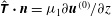
 $$\begin{eqnarray}D=\frac{k_{B}T}{6{\rm\pi}{\it\mu}_{1}af({\it\Theta},{\it\mu}_{2}/{\it\mu}_{1})}.\end{eqnarray}$$
By the index 1 we denote the fluid with the higher viscosity
 ${\it\mu}_{1}$
, while index 2 denotes the fluid having the lower viscosity. The three-phase contact angle
${\it\mu}_{1}$
, while index 2 denotes the fluid having the lower viscosity. The three-phase contact angle
 ${\it\Theta}$
is measured in fluid 1, cf. figure 1. In (1.1), the function
${\it\Theta}$
is measured in fluid 1, cf. figure 1. In (1.1), the function
 $f$
specifies the deviation of the drag force from the Stokes drag of a spherical particle suspended in the bulk of fluid 1. In terms of the drag force
$f$
specifies the deviation of the drag force from the Stokes drag of a spherical particle suspended in the bulk of fluid 1. In terms of the drag force
 $\boldsymbol{F}_{D}$
acting on the attached particle,
$\boldsymbol{F}_{D}$
acting on the attached particle,
 $f$
is thus defined by
$f$
is thus defined by
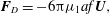 $$\begin{eqnarray}\boldsymbol{F}_{D}=-6{\rm\pi}{\it\mu}_{1}af\boldsymbol{U},\end{eqnarray}$$
where
 $\boldsymbol{U}$
denotes the particle velocity relative to the undisturbed fluids. Even when the modified Stokes–Einstein relation (1.1) is valid, as we shall assume in this study, the functional form of the drag coefficient
$\boldsymbol{U}$
denotes the particle velocity relative to the undisturbed fluids. Even when the modified Stokes–Einstein relation (1.1) is valid, as we shall assume in this study, the functional form of the drag coefficient
 $f$
of a translating interfacial particle is not known. Especially the dependence of
$f$
of a translating interfacial particle is not known. Especially the dependence of
 $f$
on
$f$
on
 ${\it\Theta}$
could help explain experimental data showing an unexpected scaling of
${\it\Theta}$
could help explain experimental data showing an unexpected scaling of
 $f$
with the particle size (Wang et al.
Reference Wang, Yordanov, Paroor, Mukhopadhyay, Li, Butt and Koynov2011; Du et al.
Reference Du, Liddle and Berglund2012), since
$f$
with the particle size (Wang et al.
Reference Wang, Yordanov, Paroor, Mukhopadhyay, Li, Butt and Koynov2011; Du et al.
Reference Du, Liddle and Berglund2012), since
 ${\it\Theta}$
is modified by line-tension effects, which become especially prominent on small scales. A variety of theoretical and experimental studies deal with the drag coefficient of particles attached to fluid–fluid interfaces (Fulford & Blake Reference Fulford and Blake1986; O’Neill, Ranger & Brenner Reference O’Neill, Ranger and Brenner1986; Danov et al.
Reference Danov, Aust, Durst and Lange1995, Reference Danov, Gurkov, Raszillier and Durst1998; Petkov et al.
Reference Petkov, Denkov, Danov, Velev, Aust and Durst1995; Cichocki et al.
Reference Cichocki, Ekiel-Jeewska, Nägele and Wajnryb2004; Fischer, Dhar & Heinig Reference Fischer, Dhar and Heinig2006; Pozrikidis Reference Pozrikidis2007; Ally & Amirfazli Reference Ally and Amirfazli2010; Bławzdziewicz, Ekiel-Jeżewska & Wajnryb Reference Bławzdziewicz, Ekiel-Jeżewska and Wajnryb2010). However, the corresponding theoretical models mostly rely on numerical methods.
${\it\Theta}$
is modified by line-tension effects, which become especially prominent on small scales. A variety of theoretical and experimental studies deal with the drag coefficient of particles attached to fluid–fluid interfaces (Fulford & Blake Reference Fulford and Blake1986; O’Neill, Ranger & Brenner Reference O’Neill, Ranger and Brenner1986; Danov et al.
Reference Danov, Aust, Durst and Lange1995, Reference Danov, Gurkov, Raszillier and Durst1998; Petkov et al.
Reference Petkov, Denkov, Danov, Velev, Aust and Durst1995; Cichocki et al.
Reference Cichocki, Ekiel-Jeewska, Nägele and Wajnryb2004; Fischer, Dhar & Heinig Reference Fischer, Dhar and Heinig2006; Pozrikidis Reference Pozrikidis2007; Ally & Amirfazli Reference Ally and Amirfazli2010; Bławzdziewicz, Ekiel-Jeżewska & Wajnryb Reference Bławzdziewicz, Ekiel-Jeżewska and Wajnryb2010). However, the corresponding theoretical models mostly rely on numerical methods.

Figure 1. Geometrical conventions used in §§ 2 and 3, respectively. The dash-dotted lines represent the planar fluid–fluid interface, while the origins of the respective coordinate systems are marked by
 $\times$
. The three-phase contact angle is measured in the upper fluid 1. Dashed arrows indicate the direction of positive torques
$\times$
. The three-phase contact angle is measured in the upper fluid 1. Dashed arrows indicate the direction of positive torques
 $M_{{\rm\pi}/2}$
and
$M_{{\rm\pi}/2}$
and
 $M_{{\rm\pi}}$
. The particle is moving to the right.
$M_{{\rm\pi}}$
. The particle is moving to the right.
With this work, we intend to contribute to the field by providing an explicit analytical expression for the drag coefficient of a spherical particle attached to a pure interface between two fluids of very different viscosity in the limit of low Reynolds number. The derived expression can be viewed as a generalization of the Stokes drag formula valid for all contact angles between the three phases. According to the Stokes–Einstein relation (1.1), the diffusion coefficient
 $D$
directly follows from the drag coefficient
$D$
directly follows from the drag coefficient
 $f$
. The work is based on a recent article Dörr & Hardt (Reference Dörr and Hardt2015) in which the flow field around a sphere attached to a fluid interface with a contact angle of
$f$
. The work is based on a recent article Dörr & Hardt (Reference Dörr and Hardt2015) in which the flow field around a sphere attached to a fluid interface with a contact angle of
 $90^{\circ }$
was computed to obtain the deformation of the interface. These earlier results are complemented by a second perturbation expansion around a contact angle of
$90^{\circ }$
was computed to obtain the deformation of the interface. These earlier results are complemented by a second perturbation expansion around a contact angle of
 $180^{\circ }$
. Based on these perturbation expansions, the Lorentz reciprocal theorem allows us to obtain the drag coefficient of the particle with high accuracy. The derived expression agrees well with the numerical results of Zabarankin (Reference Zabarankin2007), obtained for contact angles below
$180^{\circ }$
. Based on these perturbation expansions, the Lorentz reciprocal theorem allows us to obtain the drag coefficient of the particle with high accuracy. The derived expression agrees well with the numerical results of Zabarankin (Reference Zabarankin2007), obtained for contact angles below
 $90^{\circ }$
, and it goes beyond these by covering the full range of contact angles.
$90^{\circ }$
, and it goes beyond these by covering the full range of contact angles.
2 Geometric expansion around a contact angle of
 $90^{\circ }$

2.1 Series expansion of the flow field
Our modelling focuses on the drag coefficient of a rigid sphere translating along a fluid–fluid interface at low Reynolds number. We study the fundamental case of a clean fluid–fluid interface. Therefore, we do not employ any incompressibility constraint for the interface and assume a vanishing interfacial viscosity. Also, we neglect any deformation of the fluid–fluid interface on the scale of the particle radius
 $a$
, corresponding to a negligible influence of external forces acting normal to the fluid–fluid interface, such as buoyancy or electromagnetic forces. Assuming a planar interface also implies that the capillary number
$a$
, corresponding to a negligible influence of external forces acting normal to the fluid–fluid interface, such as buoyancy or electromagnetic forces. Assuming a planar interface also implies that the capillary number
 $Ca={\it\mu}_{1}U/{\it\sigma}$
(with
$Ca={\it\mu}_{1}U/{\it\sigma}$
(with
 $U=\Vert \boldsymbol{U}\Vert$
and the fluid–fluid interfacial tension
$U=\Vert \boldsymbol{U}\Vert$
and the fluid–fluid interfacial tension
 ${\it\sigma}$
), measuring dynamic deformations of the fluid–fluid interface, is small compared to unity (Radoev, Nedjalkov & Djakovich Reference Radoev, Nedjalkov and Djakovich1992).
${\it\sigma}$
), measuring dynamic deformations of the fluid–fluid interface, is small compared to unity (Radoev, Nedjalkov & Djakovich Reference Radoev, Nedjalkov and Djakovich1992).
In addition to interfacial deformations, we neglect particle rotation. The validity of this assumption depends on the conditions at the three-phase contact line, for which two limiting cases exist. Firstly, the contact line can be pinned to defects of the particle surface, meaning that it retains a fixed position with respect to the latter. A pinned contact line prevents the particle from rotating if the capillary forces due to the fluid–fluid interface are sufficiently large. Secondly, the contact line can move tangentially to the particle surface if the contact angle hysteresis is small or vanishes. In this case, the particle may rotate with an angular velocity
 $\boldsymbol{{\it\Omega}}$
dependent on the rate of dissipation occurring at the contact line. In a hydrodynamic picture the rate of dissipation is related to the extent of velocity slip at the solid surface. The model presented in this paper, relying on contact line pinning, can still be applicable to a rotating particle with a moving contact line. If the angular speed
$\boldsymbol{{\it\Omega}}$
dependent on the rate of dissipation occurring at the contact line. In a hydrodynamic picture the rate of dissipation is related to the extent of velocity slip at the solid surface. The model presented in this paper, relying on contact line pinning, can still be applicable to a rotating particle with a moving contact line. If the angular speed
 ${\it\Omega}$
is negligible compared to
${\it\Omega}$
is negligible compared to
 $U/a$
, the particle may be approximately considered non-rotating, because then the particle’s surface velocity associated with the rotational motion is much smaller than the surface velocity
$U/a$
, the particle may be approximately considered non-rotating, because then the particle’s surface velocity associated with the rotational motion is much smaller than the surface velocity
 $U$
associated with the translational motion. For increasing angular velocity, that is, decreasing dissipation at the moving contact line, the assumption of a non-rotating particle loses its validity. Consequently, the following model is valid for a particle with
$U$
associated with the translational motion. For increasing angular velocity, that is, decreasing dissipation at the moving contact line, the assumption of a non-rotating particle loses its validity. Consequently, the following model is valid for a particle with
 ${\it\Omega}a/U\ll 1$
.
${\it\Omega}a/U\ll 1$
.
To further simplify the mathematical treatment, we assume a vanishing viscosity ratio between the two fluids,
 ${\it\mu}_{2}/{\it\mu}_{1}\rightarrow 0$
. As a consequence of this assumption, the condition of tangential stress being continuous upon crossing the fluid interface is simplified to a condition of vanishing tangential stress exerted upon the fluid interface by fluid 1. Thus the planar fluid–fluid interface effectively becomes a symmetry plane from the viewpoint of fluid 1, while the influence of fluid 2 can be neglected. For this reason, the flow problem is analogous to the motion of a body possessing reflection symmetry moving parallel to its symmetry plane. Clearly, for a contact angle
${\it\mu}_{2}/{\it\mu}_{1}\rightarrow 0$
. As a consequence of this assumption, the condition of tangential stress being continuous upon crossing the fluid interface is simplified to a condition of vanishing tangential stress exerted upon the fluid interface by fluid 1. Thus the planar fluid–fluid interface effectively becomes a symmetry plane from the viewpoint of fluid 1, while the influence of fluid 2 can be neglected. For this reason, the flow problem is analogous to the motion of a body possessing reflection symmetry moving parallel to its symmetry plane. Clearly, for a contact angle
 ${\it\Theta}$
of
${\it\Theta}$
of
 $90^{\circ }$
, the symmetric body is spherical, resulting in the classical Stokes flow problem around a sphere. The corresponding drag on an interfacial particle is then simply half the Stokes drag in the bulk of fluid 1 (Ranger Reference Ranger1978; O’Neill et al.
Reference O’Neill, Ranger and Brenner1986; Radoev et al.
Reference Radoev, Nedjalkov and Djakovich1992; Danov et al.
Reference Danov, Aust, Durst and Lange1995; Petkov et al.
Reference Petkov, Denkov, Danov, Velev, Aust and Durst1995; Ally & Amirfazli Reference Ally and Amirfazli2010), implying
$90^{\circ }$
, the symmetric body is spherical, resulting in the classical Stokes flow problem around a sphere. The corresponding drag on an interfacial particle is then simply half the Stokes drag in the bulk of fluid 1 (Ranger Reference Ranger1978; O’Neill et al.
Reference O’Neill, Ranger and Brenner1986; Radoev et al.
Reference Radoev, Nedjalkov and Djakovich1992; Danov et al.
Reference Danov, Aust, Durst and Lange1995; Petkov et al.
Reference Petkov, Denkov, Danov, Velev, Aust and Durst1995; Ally & Amirfazli Reference Ally and Amirfazli2010), implying
 $$\begin{eqnarray}f(90^{\circ },0)=1/2,\end{eqnarray}$$
where the function
 $f$
is defined by (1.1).
$f$
is defined by (1.1).

Figure 2. Pair of flow problems connected by the Lorentz reciprocal theorem (2.16). (a) A sphere moving along a fluid–fluid interface with vanishing viscosity ratio causes a flow field identical to the classical Stokes flow problem in a bulk fluid, denoted by
 $\hat{\boldsymbol{u}}$
and
$\hat{\boldsymbol{u}}$
and
 $\hat{\boldsymbol{\unicode[STIX]{x1D64F}}}$
, if the contact angle
$\hat{\boldsymbol{\unicode[STIX]{x1D64F}}}$
, if the contact angle
 ${\it\Theta}$
equals
${\it\Theta}$
equals
 $90^{\circ }$
. (b) For
$90^{\circ }$
. (b) For
 ${\it\Theta}\neq 90^{\circ }$
, the flow problem is equivalent to a pair of fused spheres moving through a bulk fluid. By means of a perturbation expansion, the boundary condition on the complex particle surface is projected onto a sphere and the flow field in this case is denoted by
${\it\Theta}\neq 90^{\circ }$
, the flow problem is equivalent to a pair of fused spheres moving through a bulk fluid. By means of a perturbation expansion, the boundary condition on the complex particle surface is projected onto a sphere and the flow field in this case is denoted by
 $\boldsymbol{u}$
and
$\boldsymbol{u}$
and
 $\boldsymbol{\unicode[STIX]{x1D64F}}$
.
$\boldsymbol{\unicode[STIX]{x1D64F}}$
.
For contact angles differing from
 $90^{\circ }$
, the symmetric body consists of two fused spheres (cf. figure 2
b). This case has been studied by Zabarankin (Reference Zabarankin2007), who provides drag coefficient values derived from a numerical solution of a Fredholm integral equation. Recently, Dörr & Hardt (Reference Dörr and Hardt2015) have derived the asymptotic expression
$90^{\circ }$
, the symmetric body consists of two fused spheres (cf. figure 2
b). This case has been studied by Zabarankin (Reference Zabarankin2007), who provides drag coefficient values derived from a numerical solution of a Fredholm integral equation. Recently, Dörr & Hardt (Reference Dörr and Hardt2015) have derived the asymptotic expression
 $$\begin{eqnarray}f({\it\Theta},0)={\textstyle \frac{1}{2}}\left[1+{\textstyle \frac{9}{16}}\cos {\it\Theta}+O(\cos ^{2}{\it\Theta})\right].\end{eqnarray}$$
The result (2.2) has been obtained following a method of Brenner (Reference Brenner1964) (cf. Dörr & Hardt Reference Dörr and Hardt2015) concerning necessary corrections to the method), which is based on spherical harmonics expansions and yields the velocity and pressure fields around a slightly deformed sphere. To this end, the particle shape (given by the pair of fused spheres of radius
 $a$
in our case) needs to be parameterised in spherical coordinates
$a$
in our case) needs to be parameterised in spherical coordinates
 $(r,{\it\theta},{\it\varphi})$
, with the origin lying in the particle’s symmetry plane, according to
$(r,{\it\theta},{\it\varphi})$
, with the origin lying in the particle’s symmetry plane, according to
 $$\begin{eqnarray}r=r_{p}({\it\theta},{\it\varphi}),\end{eqnarray}$$
and subsequently expanded in a power series
 $$\begin{eqnarray}r_{p}({\it\theta},{\it\varphi})=a[1+{\it\varepsilon}{\it\phi}^{(1)}({\it\theta},{\it\varphi})+{\it\varepsilon}^{2}{\it\phi}^{(2)}({\it\theta},{\it\varphi})+\cdots \,]\end{eqnarray}$$
in terms of a small parameter
 ${\it\varepsilon}$
. Here, we choose
${\it\varepsilon}$
. Here, we choose
 ${\it\varepsilon}=\cos {\it\Theta}$
, so that
${\it\varepsilon}=\cos {\it\Theta}$
, so that
 $2{\it\varepsilon}a$
equals the distance between the centres of the fused spheres (cf. figure 1
a). Accordingly, if we assume the centres of the spheres to lie on the
$2{\it\varepsilon}a$
equals the distance between the centres of the fused spheres (cf. figure 1
a). Accordingly, if we assume the centres of the spheres to lie on the
 $x$
-axis with the symmetry plane given by
$x$
-axis with the symmetry plane given by
 $x=0$
, the particle shape is described by
$x=0$
, the particle shape is described by
 $$\begin{eqnarray}r_{p}({\it\theta},{\it\varphi})=a\left[1+{\it\varepsilon}\sin {\it\theta}\left|\cos {\it\varphi}\right|+{\it\varepsilon}^{2}\left(\frac{\sin ^{2}{\it\theta}\cos ^{2}{\it\varphi}-1}{2}\right)+\cdots \,\right],\end{eqnarray}$$
from which the functions
 ${\it\phi}^{(1)}$
and
${\it\phi}^{(1)}$
and
 ${\it\phi}^{(2)}$
in (2.4) can be read.
${\it\phi}^{(2)}$
in (2.4) can be read.
At the same time, the velocity and pressure fields,
 $\boldsymbol{u}$
and
$\boldsymbol{u}$
and
 $p$
, are written in the form
$p$
, are written in the form
 $$\begin{eqnarray}\displaystyle \displaystyle \boldsymbol{u} & = & \displaystyle \boldsymbol{u}^{(0)}+{\it\varepsilon}\boldsymbol{u}^{(1)}+{\it\varepsilon}^{2}\boldsymbol{u}^{(2)}+O({\it\varepsilon}^{3}),\quad \text{and}\end{eqnarray}$$
 $$\begin{eqnarray}\displaystyle \displaystyle \boldsymbol{p} & = & \displaystyle p^{(0)}+{\it\varepsilon}p^{(1)}+{\it\varepsilon}^{2}p^{(2)}+O({\it\varepsilon}^{3}).\end{eqnarray}$$
 $\boldsymbol{U}$
. Therefore, the flow field obeys the boundary conditions
$\boldsymbol{U}$
. Therefore, the flow field obeys the boundary conditions  $$\begin{eqnarray}\left.\boldsymbol{u}\right|_{{\it\Sigma}_{p}}=\boldsymbol{U}\end{eqnarray}$$
at the particle surface
 ${\it\Sigma}_{p}$
, and
${\it\Sigma}_{p}$
, and
 $$\begin{eqnarray}\left.\boldsymbol{u}\right|_{{\it\Sigma}_{\infty }}=\mathbf{0}\end{eqnarray}$$
on a spherical surface
 ${\it\Sigma}_{\infty }$
at
${\it\Sigma}_{\infty }$
at
 $r\rightarrow \infty$
. While condition (2.9) is readily adapted to the perturbation expansion (2.6), condition (2.8) on the particle surface requires a Taylor series expansion for removal of the implicit dependence on the shape parameter
$r\rightarrow \infty$
. While condition (2.9) is readily adapted to the perturbation expansion (2.6), condition (2.8) on the particle surface requires a Taylor series expansion for removal of the implicit dependence on the shape parameter
 ${\it\varepsilon}$
. To be precise, the boundary condition (2.8) in conjunction with the expanded particle shape (2.4) reads
${\it\varepsilon}$
. To be precise, the boundary condition (2.8) in conjunction with the expanded particle shape (2.4) reads
 $$\begin{eqnarray}\boldsymbol{u}(r_{p},{\it\theta},{\it\varphi})=\boldsymbol{U},\end{eqnarray}$$
which equals
 $$\begin{eqnarray}\boldsymbol{u}^{(0)}(r_{p},{\it\theta},{\it\varphi})+{\it\varepsilon}\boldsymbol{u}^{(1)}(r_{p},{\it\theta},{\it\varphi})+{\it\varepsilon}^{2}\boldsymbol{u}^{(2)}(r_{p},{\it\theta},{\it\varphi})+O({\it\varepsilon}^{3})=\boldsymbol{U}.\end{eqnarray}$$
In (2.11), the argument
 $r_{p}$
depends on
$r_{p}$
depends on
 ${\it\varepsilon}$
, so that the velocity vectors
${\it\varepsilon}$
, so that the velocity vectors
 $\boldsymbol{u}^{(i)}~(i\in \{0,1,2\})$
are to be expanded in a Taylor series about
$\boldsymbol{u}^{(i)}~(i\in \{0,1,2\})$
are to be expanded in a Taylor series about
 $r=a$
in powers of
$r=a$
in powers of
 ${\it\varepsilon}$
, using (2.4). After performing the expansions, inserting the results into (2.11) and grouping of terms, we arrive at
${\it\varepsilon}$
, using (2.4). After performing the expansions, inserting the results into (2.11) and grouping of terms, we arrive at
 $$\begin{eqnarray}\displaystyle \left.\begin{array}{@{}c@{}}\displaystyle \boldsymbol{u}^{(0)}=\boldsymbol{U}\\ \displaystyle \boldsymbol{u}^{(1)}=-a{\it\phi}^{(1)}\frac{\partial \boldsymbol{u}^{(0)}}{\partial r}\\ \displaystyle \boldsymbol{u}^{(2)}=-a{\it\phi}^{(2)}\frac{\partial \boldsymbol{u}^{(0)}}{\partial r}-\frac{a^{2}}{2}\left[{\it\phi}^{(1)}\right]^{2}\frac{\partial ^{2}\boldsymbol{u}^{(0)}}{\partial r^{2}}-a{\it\phi}^{(1)}\frac{\partial \boldsymbol{u}^{(1)}}{\partial r}\end{array}\right\}\quad \text{at }r=a. & & \displaystyle\end{eqnarray}$$
Clearly, the zeroth-order problem corresponds to a spherical particle moving with constant velocity
 $\boldsymbol{U}$
in an unbounded fluid, for which the velocity and pressure fields
$\boldsymbol{U}$
in an unbounded fluid, for which the velocity and pressure fields
 $$\begin{eqnarray}\displaystyle \boldsymbol{u}^{(0)}=-\frac{1}{2}U\left(\frac{a}{r}\right)^{2}\left(\frac{a}{r}-3\frac{r}{a}\right)\cos {\it\theta}\boldsymbol{e}_{r}-\frac{1}{4}U\left(\frac{a}{r}\right)^{2}\left(\frac{a}{r}+3\frac{r}{a}\right)\sin {\it\theta}\boldsymbol{e}_{{\it\theta}}, & & \displaystyle\end{eqnarray}$$
and
 $$\begin{eqnarray}\displaystyle p^{(0)}=\frac{3}{2}{\it\mu}_{1}Ua\frac{\cos {\it\theta}}{r^{2}} & & \displaystyle\end{eqnarray}$$
are well known (Happel & Brenner Reference Happel and Brenner1983). The first-order problem has been solved by Dörr & Hardt (Reference Dörr and Hardt2015) in the particle’s rest frame. Because the frame of reference only affects the zeroth-order flow
 $\boldsymbol{u}^{(0)}$
by addition or subtraction of the velocity field
$\boldsymbol{u}^{(0)}$
by addition or subtraction of the velocity field
 $\boldsymbol{U}$
, the first-order flow field
$\boldsymbol{U}$
, the first-order flow field
 $\boldsymbol{u}^{(1)}$
considered by Dörr & Hardt (Reference Dörr and Hardt2015) may be directly used in the present study. The supplementary material available at http://dx.doi.org/10.1017/jfm.2016.41 contains the complete set of expressions required to calculate the velocity field
$\boldsymbol{u}^{(1)}$
considered by Dörr & Hardt (Reference Dörr and Hardt2015) may be directly used in the present study. The supplementary material available at http://dx.doi.org/10.1017/jfm.2016.41 contains the complete set of expressions required to calculate the velocity field
 $\boldsymbol{u}^{(1)}$
. Since
$\boldsymbol{u}^{(1)}$
. Since
 $\boldsymbol{u}^{(1)}$
is equal to the infinite series
$\boldsymbol{u}^{(1)}$
is equal to the infinite series
 $\sum _{k=0}^{\infty }\boldsymbol{u}_{k}^{(1)}$
(Brenner Reference Brenner1964), the number of included terms needs to be limited in practical calculations. The values reported below as well as in the supplementary material correspond to
$\sum _{k=0}^{\infty }\boldsymbol{u}_{k}^{(1)}$
(Brenner Reference Brenner1964), the number of included terms needs to be limited in practical calculations. The values reported below as well as in the supplementary material correspond to
 $k\leqslant 20$
. With this choice, the
$k\leqslant 20$
. With this choice, the
 $O({\it\varepsilon}^{2})$
contribution to the drag coefficient can be calculated to three significant digits, as will be shown in the following section.
$O({\it\varepsilon}^{2})$
contribution to the drag coefficient can be calculated to three significant digits, as will be shown in the following section.
2.2 Applying the Lorentz reciprocal theorem
According to the above discussion, we are in a position to compute the velocity fields
 $\boldsymbol{u}^{(i)}(a,{\it\theta},{\it\varphi}),~i\in \{0,1,2\}$
, on a spherical surface by means of (2.12). In other words, we are faced with two flow problems involving a sphere of radius
$\boldsymbol{u}^{(i)}(a,{\it\theta},{\it\varphi}),~i\in \{0,1,2\}$
, on a spherical surface by means of (2.12). In other words, we are faced with two flow problems involving a sphere of radius
 $a$
in an unbounded fluid, see figure 2. The first of these problems (figure 2
a), constructed by setting
$a$
in an unbounded fluid, see figure 2. The first of these problems (figure 2
a), constructed by setting
 ${\it\varepsilon}$
to zero, consists of a sphere with a no-slip surface condition and translating with velocity
${\it\varepsilon}$
to zero, consists of a sphere with a no-slip surface condition and translating with velocity
 $\boldsymbol{U}$
. We shall denote the velocity and stress tensor fields belonging to this first problem by
$\boldsymbol{U}$
. We shall denote the velocity and stress tensor fields belonging to this first problem by
 $\hat{\boldsymbol{u}}$
and
$\hat{\boldsymbol{u}}$
and
 $\hat{\boldsymbol{\unicode[STIX]{x1D64F}}}$
, respectively. The second problem (figure 2
b), associated with the truncated perturbation expansion in
$\hat{\boldsymbol{\unicode[STIX]{x1D64F}}}$
, respectively. The second problem (figure 2
b), associated with the truncated perturbation expansion in
 ${\it\varepsilon}$
and denoted by
${\it\varepsilon}$
and denoted by
 $\boldsymbol{u}$
and
$\boldsymbol{u}$
and
 $\boldsymbol{\unicode[STIX]{x1D64F}}$
, is given by a sphere with a prescribed surface velocity field of
$\boldsymbol{\unicode[STIX]{x1D64F}}$
, is given by a sphere with a prescribed surface velocity field of
 $$\begin{eqnarray}\boldsymbol{u}(a,{\it\theta},{\it\varphi})=\mathop{\sum }_{i=0}^{\infty }{\it\varepsilon}^{i}\boldsymbol{u}^{(i)}(a,{\it\theta},{\it\varphi})=\boldsymbol{U}+{\it\varepsilon}\boldsymbol{u}^{(1)}(a,{\it\theta},{\it\varphi})+{\it\varepsilon}^{2}\boldsymbol{u}^{(2)}(a,{\it\theta},{\it\varphi})+O({\it\varepsilon}^{3}),\end{eqnarray}$$
according to (2.12).
Since the solutions
 $(\hat{\boldsymbol{u}},\hat{\boldsymbol{\unicode[STIX]{x1D64F}}})$
and
$(\hat{\boldsymbol{u}},\hat{\boldsymbol{\unicode[STIX]{x1D64F}}})$
and
 $(\boldsymbol{u},\boldsymbol{\unicode[STIX]{x1D64F}})$
correspond to the same flow geometry, they are related by the Lorentz reciprocal theorem for Stokes flow (Lorentz Reference Lorentz1896; Brenner Reference Brenner1964; Happel & Brenner Reference Happel and Brenner1983),
$(\boldsymbol{u},\boldsymbol{\unicode[STIX]{x1D64F}})$
correspond to the same flow geometry, they are related by the Lorentz reciprocal theorem for Stokes flow (Lorentz Reference Lorentz1896; Brenner Reference Brenner1964; Happel & Brenner Reference Happel and Brenner1983),
 $$\begin{eqnarray}\int _{{\it\Sigma}}\left(\hat{\boldsymbol{\unicode[STIX]{x1D64F}}}\boldsymbol{\cdot }\boldsymbol{n}\right)\boldsymbol{\cdot }\boldsymbol{u}\,\text{d}{\it\Sigma}=\int _{{\it\Sigma}}\left(\boldsymbol{\unicode[STIX]{x1D64F}}\boldsymbol{\cdot }\boldsymbol{n}\right)\boldsymbol{\cdot }\hat{\boldsymbol{u}}\,\text{d}{\it\Sigma},\end{eqnarray}$$
where
 ${\it\Sigma}$
comprises the particle surface
${\it\Sigma}$
comprises the particle surface
 ${\it\Sigma}_{p}$
(outer normal vector
${\it\Sigma}_{p}$
(outer normal vector
 $\boldsymbol{n}=-\boldsymbol{e}_{r}$
) and the surface
$\boldsymbol{n}=-\boldsymbol{e}_{r}$
) and the surface
 ${\it\Sigma}_{\infty }$
at infinity (outer normal vector
${\it\Sigma}_{\infty }$
at infinity (outer normal vector
 $\boldsymbol{n}=\boldsymbol{e}_{r}$
).
$\boldsymbol{n}=\boldsymbol{e}_{r}$
).
The application of the reciprocal theorem (2.16) to a number of problems involving the motion of particles in low Reynolds number flows has been reviewed by Leal (Reference Leal1980); for several more recent applications, see Stone & Samuel (Reference Stone and Samuel1996), Masoud & Stone (Reference Masoud and Stone2014) and Schönecker & Hardt (Reference Schönecker and Hardt2014). Its use in the present study is inspired by the works of Brenner (Reference Brenner1964) and Stone & Samuel (Reference Stone and Samuel1996). Brenner (Reference Brenner1964) showed that the drag force can be calculated to one order higher than the order to which the flow field is known. Returning to our calculation, the contribution from the integral over
 ${\it\Sigma}_{\infty }$
in (2.16) vanishes because
${\it\Sigma}_{\infty }$
in (2.16) vanishes because
 $$\begin{eqnarray}\Vert \hat{\boldsymbol{u}}\Vert \sim r^{-1},\quad \left\Vert \boldsymbol{u}\right\Vert \sim r^{-1},\quad \Vert \hat{\boldsymbol{\unicode[STIX]{x1D64F}}}\boldsymbol{\cdot }\boldsymbol{e}_{r}\Vert \sim r^{-2},\quad \text{and}\quad \left\Vert \boldsymbol{\unicode[STIX]{x1D64F}}\boldsymbol{\cdot }\boldsymbol{e}_{r}\right\Vert \sim r^{-2}\quad \text{for}~r\rightarrow \infty .\end{eqnarray}$$
The integral in (2.16) thus reduces to an integral over the particle surface
 ${\it\Sigma}_{p}$
. Recalling that
${\it\Sigma}_{p}$
. Recalling that
 $\hat{\boldsymbol{\unicode[STIX]{x1D64F}}}\boldsymbol{\cdot }\boldsymbol{n}=-\hat{\boldsymbol{\unicode[STIX]{x1D64F}}}\boldsymbol{\cdot }\boldsymbol{e}_{r}=3{\it\mu}_{1}\boldsymbol{U}/(2a)$
(Stone & Samuel Reference Stone and Samuel1996) and using (2.15), the reciprocal theorem can be written as
$\hat{\boldsymbol{\unicode[STIX]{x1D64F}}}\boldsymbol{\cdot }\boldsymbol{n}=-\hat{\boldsymbol{\unicode[STIX]{x1D64F}}}\boldsymbol{\cdot }\boldsymbol{e}_{r}=3{\it\mu}_{1}\boldsymbol{U}/(2a)$
(Stone & Samuel Reference Stone and Samuel1996) and using (2.15), the reciprocal theorem can be written as
 $$\begin{eqnarray}\int _{{\it\Sigma}_{p}}\frac{3{\it\mu}_{1}}{2a}\boldsymbol{U}\boldsymbol{\cdot }\left[\boldsymbol{U}+{\it\varepsilon}\boldsymbol{u}^{(1)}+{\it\varepsilon}^{2}\boldsymbol{u}^{(2)}+O({\it\varepsilon}^{3})\right]\,\text{d}{\it\Sigma}=\int _{{\it\Sigma}_{p}}\left(\boldsymbol{\unicode[STIX]{x1D64F}}\boldsymbol{\cdot }\boldsymbol{n}\right)\boldsymbol{\cdot }\boldsymbol{U}\,\text{d}{\it\Sigma}.\end{eqnarray}$$
Since
 $\boldsymbol{U}$
is a constant vector and
$\boldsymbol{U}$
is a constant vector and
 $\int _{{\it\Sigma}_{p}}\,\text{d}{\it\Sigma}=4{\rm\pi}a^{2}$
, (2.18) simplifies to
$\int _{{\it\Sigma}_{p}}\,\text{d}{\it\Sigma}=4{\rm\pi}a^{2}$
, (2.18) simplifies to
 $$\begin{eqnarray}6{\rm\pi}{\it\mu}_{1}U^{2}+\frac{3{\it\mu}_{1}}{2a}\boldsymbol{U}\boldsymbol{\cdot }\int _{{\it\Sigma}_{p}}\left[{\it\varepsilon}\boldsymbol{u}^{(1)}+{\it\varepsilon}^{2}\boldsymbol{u}^{(2)}+O({\it\varepsilon}^{3})\right]\,\text{d}{\it\Sigma}=\boldsymbol{U}\boldsymbol{\cdot }\underbrace{\int _{{\it\Sigma}_{p}}\boldsymbol{\unicode[STIX]{x1D64F}}\boldsymbol{\cdot }\boldsymbol{n}\,\text{d}{\it\Sigma}}_{=-\boldsymbol{F}_{D}}.\end{eqnarray}$$
The integral on the right-hand side of (2.19) has been identified with the negative of the Stokes drag
 $\boldsymbol{F}_{D}$
on the particle because
$\boldsymbol{F}_{D}$
on the particle because
 $\boldsymbol{n}=-\boldsymbol{e}_{r}$
. Then, using (2.12), (2.13), (2.4) and (2.5) in conjunction with the velocity field
$\boldsymbol{n}=-\boldsymbol{e}_{r}$
. Then, using (2.12), (2.13), (2.4) and (2.5) in conjunction with the velocity field
 $\boldsymbol{u}^{(1)}$
according to Dörr & Hardt (Reference Dörr and Hardt2015), the integral occurring in (2.19) can be evaluated, yielding
$\boldsymbol{u}^{(1)}$
according to Dörr & Hardt (Reference Dörr and Hardt2015), the integral occurring in (2.19) can be evaluated, yielding
 $$\begin{eqnarray}\boldsymbol{F}_{D}=-6{\rm\pi}{\it\mu}_{1}a\boldsymbol{U}[1+{\textstyle \frac{9}{16}}{\it\varepsilon}-0.139{\it\varepsilon}^{2}+O({\it\varepsilon}^{3})].\end{eqnarray}$$
Thus, the drag coefficient (1.2) for the original problem of a spherical particle diffusing along a fluid–fluid interface of zero viscosity ratio is given by
 $$\begin{eqnarray}f_{{\rm\pi}/2}({\it\Theta},0)={\textstyle \frac{1}{2}}[1+{\textstyle \frac{9}{16}}\cos {\it\Theta}-0.139\cos ^{2}{\it\Theta}+O(\cos ^{3}{\it\Theta})].\end{eqnarray}$$
Correspondingly, for the diffusion coefficient (1.1) it follows that
 $$\begin{eqnarray}D=\frac{16k_{B}T}{3{\rm\pi}{\it\mu}_{1}a\left[16+9\cos {\it\Theta}-2.224\cos ^{2}{\it\Theta}+O(\cos ^{3}{\it\Theta})\right]}.\end{eqnarray}$$
Note that the numerical coefficient 0.139 in (2.21) can be calculated to any desired number of significant digits, provided that a sufficient number of terms is considered in the spherical harmonics expansion by Brenner (Reference Brenner1964) and Dörr & Hardt (Reference Dörr and Hardt2015). As stated above, the value
 $0.139\ldots \approx 765\,368\,413\,099/5497\,558\,138\,880$
corresponds to 20 terms. The torque
$0.139\ldots \approx 765\,368\,413\,099/5497\,558\,138\,880$
corresponds to 20 terms. The torque
 $M_{{\rm\pi}/2}$
acting on the particle in the direction indicated in figure 1(a) was calculated by Dörr & Hardt (Reference Dörr and Hardt2015) (cf. (3.24) and (4.19) therein) as
$M_{{\rm\pi}/2}$
acting on the particle in the direction indicated in figure 1(a) was calculated by Dörr & Hardt (Reference Dörr and Hardt2015) (cf. (3.24) and (4.19) therein) as
 $$\begin{eqnarray}M_{{\rm\pi}/2}={\rm\pi}{\it\mu}_{1}a^{2}U[{\textstyle \frac{3}{2}}+2.863\cos {\it\Theta}+O(\cos ^{2}{\it\Theta})].\end{eqnarray}$$
3 Geometric expansion around a contact angle of
$180^{\circ }$

3.1 Series expansion of the flow field
For contact angles
 ${\it\Theta}$
close to
${\it\Theta}$
close to
 $180^{\circ }$
(
$180^{\circ }$
(
 ${\rm\pi}-{\it\Theta}\ll 1$
), the symmetric body takes the form of a lens (see figure 1
b). Therefore, it is more realistic to describe the body shape in terms of a perturbation expansion from a circular disk. Let
${\rm\pi}-{\it\Theta}\ll 1$
), the symmetric body takes the form of a lens (see figure 1
b). Therefore, it is more realistic to describe the body shape in terms of a perturbation expansion from a circular disk. Let
 $(r,{\it\theta},z)$
be cylindrical coordinates, where
$(r,{\it\theta},z)$
be cylindrical coordinates, where
 $z=0$
represents the interface and
$z=0$
represents the interface and
 $r=0$
passes through the centre of the lens. In these coordinates, the surface of the symmetric particle can be described as
$r=0$
passes through the centre of the lens. In these coordinates, the surface of the symmetric particle can be described as
 $$\begin{eqnarray}z=\pm \frac{R}{\sin {\it\Theta}}\left[\sqrt{1-\left(\frac{r}{R}\right)^{2}\sin ^{2}{\it\Theta}}+\cos {\it\Theta}\right]=\pm R[{\it\varepsilon}{\it\phi}\left(r\right)+O\left({\it\varepsilon}^{2}\right)],\end{eqnarray}$$
where
 $R=a\sin {\it\Theta}$
is the radius of the three-phase contact line,
$R=a\sin {\it\Theta}$
is the radius of the three-phase contact line,
 ${\it\varepsilon}=z_{max}/R=\cot \left({\it\Theta}/2\right)$
is the aspect ratio of the lens, and
${\it\varepsilon}=z_{max}/R=\cot \left({\it\Theta}/2\right)$
is the aspect ratio of the lens, and
 ${\it\phi}\left(r\right)=1-\left(r/R\right)^{2}$
. It is then natural to write the velocity and pressure in the form
${\it\phi}\left(r\right)=1-\left(r/R\right)^{2}$
. It is then natural to write the velocity and pressure in the form
 $$\begin{eqnarray}\displaystyle \displaystyle \boldsymbol{u} & \hspace{-2.0pt}=\hspace{-2.0pt} & \displaystyle \boldsymbol{u}^{(0)}+{\it\varepsilon}\boldsymbol{u}^{(1)}+O({\it\varepsilon}^{2}),\quad \text{and}\end{eqnarray}$$
 $$\begin{eqnarray}\displaystyle \displaystyle p & \hspace{-2.0pt}=\hspace{-2.0pt} & \displaystyle p^{(0)}+{\it\varepsilon}p^{(1)}+O({\it\varepsilon}^{2}).\end{eqnarray}$$
 ${\it\varepsilon}$
,
${\it\varepsilon}$
,
 $r$
, and
$r$
, and
 ${\it\phi}\left(r\right)$
have different definitions than in the previous section.
${\it\phi}\left(r\right)$
have different definitions than in the previous section.
To proceed, we represent the boundary conditions at the actual surface of the particle in terms of a Taylor series about
 $z=0$
, similar to what was done in § 2.1. Hence, the velocity at
$z=0$
, similar to what was done in § 2.1. Hence, the velocity at
 $z=0$
is given by
$z=0$
is given by
 $$\begin{eqnarray}\boldsymbol{u}=\boldsymbol{u}^{\left(0\right)}+{\it\varepsilon}\left[\boldsymbol{u}^{\left(1\right)}+R{\it\phi}\left(r\right)\frac{\partial \boldsymbol{u}^{\left(0\right)}}{\partial z}\right]+O({\it\varepsilon}^{2}).\end{eqnarray}$$
All boundary conditions from now on are applied at
 $z=0$
. At
$z=0$
. At
 $O\left(1\right)$
, we must solve for the edgewise translation of a circular disk with the boundary condition
$O\left(1\right)$
, we must solve for the edgewise translation of a circular disk with the boundary condition
 $$\begin{eqnarray}\boldsymbol{u}^{\left(0\right)}=\boldsymbol{U}\quad \text{at }z=0~(r\leqslant R).\end{eqnarray}$$
At
 $O\left({\it\varepsilon}\right)$
, the flow must satisfy
$O\left({\it\varepsilon}\right)$
, the flow must satisfy
 $$\begin{eqnarray}\boldsymbol{u}^{\left(1\right)}=-R{\it\phi}\left(r\right)\frac{\partial \boldsymbol{u}^{\left(0\right)}}{\partial z}\quad \text{at}~z=0~(r\leqslant R).\end{eqnarray}$$
At all orders, the flow vanishes at infinity.
3.2 Applying the Lorentz reciprocal theorem
Applying the reciprocal theorem (2.16), we obtain
 $$\begin{eqnarray}\int _{{\it\Sigma}_{p}}(\hat{\boldsymbol{\unicode[STIX]{x1D64F}}}\boldsymbol{\cdot }\boldsymbol{n})\boldsymbol{\cdot }[\boldsymbol{u}^{\left(0\right)}+{\it\varepsilon}\boldsymbol{u}^{\left(1\right)}+O({\it\varepsilon}^{2})]\,\text{d}S=\boldsymbol{F}_{D}\boldsymbol{\cdot }\boldsymbol{U},\end{eqnarray}$$
where
 ${\it\Sigma}_{p}$
denotes the surface of the disk (
${\it\Sigma}_{p}$
denotes the surface of the disk (
 $z=0,\;r\leqslant R$
) and
$z=0,\;r\leqslant R$
) and
 $\boldsymbol{n}=\pm \boldsymbol{e}_{z}$
. As above, the integrals over
$\boldsymbol{n}=\pm \boldsymbol{e}_{z}$
. As above, the integrals over
 ${\it\Sigma}_{\infty }$
are zero (see (2.17)). Applying the boundary conditions (3.5) and (3.6) and replacing
${\it\Sigma}_{\infty }$
are zero (see (2.17)). Applying the boundary conditions (3.5) and (3.6) and replacing
 $\hat{\boldsymbol{\unicode[STIX]{x1D64F}}}\boldsymbol{\cdot }\boldsymbol{n}={\it\mu}_{1}\partial \boldsymbol{u}^{(0)}/\partial z$
, (3.7) reduces to (accounting for both sides of the disk)
$\hat{\boldsymbol{\unicode[STIX]{x1D64F}}}\boldsymbol{\cdot }\boldsymbol{n}={\it\mu}_{1}\partial \boldsymbol{u}^{(0)}/\partial z$
, (3.7) reduces to (accounting for both sides of the disk)
 $$\begin{eqnarray}\boldsymbol{F}_{D}\boldsymbol{\cdot }\boldsymbol{U}=-\frac{32}{3}{\it\mu}_{1}RU^{2}-2{\it\mu}_{1}R{\it\varepsilon}\int _{r=0}^{R}\int _{{\it\theta}=0}^{2{\rm\pi}}{\it\phi}\left(r\right)\left(\frac{\partial \boldsymbol{u}^{\left(0\right)}}{\partial z}\right)^{2}\;r\,\text{d}r\,\text{d}{\it\theta}+O\left({\it\varepsilon}^{2}\right).\end{eqnarray}$$
The ideas used to derive (3.8) are also useful in analysing the motion of a particle at a surfactant-covered interface (Stone & Masoud Reference Stone and Masoud2015).
The velocity field
 $\boldsymbol{u}^{(0)}$
for flow about a circular disk translating edgewise is known analytically (e.g. Ranger Reference Ranger1978; Davis Reference Davis1990; Tanzosh & Stone Reference Tanzosh and Stone1996):
$\boldsymbol{u}^{(0)}$
for flow about a circular disk translating edgewise is known analytically (e.g. Ranger Reference Ranger1978; Davis Reference Davis1990; Tanzosh & Stone Reference Tanzosh and Stone1996):
 $$\begin{eqnarray}\displaystyle & \displaystyle u_{r}^{(0)}(r,{\it\theta},z)=\frac{2U\cos {\it\theta}}{3{\rm\pi}}\left[3\cot ^{-1}{\it\lambda}-\frac{{\it\lambda}{\it\zeta}^{2}}{{\it\lambda}^{2}+{\it\zeta}^{2}}+\frac{{\it\lambda}^{3}(1-{\it\zeta}^{2})}{(1+{\it\lambda}^{2})({\it\lambda}^{2}+{\it\zeta}^{2})}\right], & \displaystyle\end{eqnarray}$$
 $$\begin{eqnarray}\displaystyle & \displaystyle u_{{\it\theta}}^{(0)}(r,{\it\theta},z)=\frac{2U\sin {\it\theta}}{3{\rm\pi}}\left[-3\cot ^{-1}{\it\lambda}+\frac{{\it\lambda}{\it\zeta}^{2}}{{\it\lambda}^{2}+{\it\zeta}^{2}}+\frac{{\it\lambda}^{3}(1-{\it\zeta}^{2})}{(1+{\it\lambda}^{2})({\it\lambda}^{2}+{\it\zeta}^{2})}\right], & \displaystyle\end{eqnarray}$$
 ${\it\lambda}$
and
${\it\lambda}$
and
 ${\it\zeta}$
are the oblate spheroidal coordinates defined via
${\it\zeta}$
are the oblate spheroidal coordinates defined via
 $z=R{\it\lambda}{\it\zeta}$
and
$z=R{\it\lambda}{\it\zeta}$
and
 $r^{2}=R^{2}(1+{\it\lambda}^{2})(1-{\it\zeta}^{2})$
, with
$r^{2}=R^{2}(1+{\it\lambda}^{2})(1-{\it\zeta}^{2})$
, with
 $0\leqslant {\it\zeta}<1$
. After
$0\leqslant {\it\zeta}<1$
. After
 ${\it\theta}$
integration, the integration in
${\it\theta}$
integration, the integration in
 $r$
(at
$r$
(at
 $z=0$
) is accomplished by transforming to
$z=0$
) is accomplished by transforming to
 ${\it\zeta}$
. Substituting
${\it\zeta}$
. Substituting
 $\partial \boldsymbol{u}^{\left(0\right)}/\partial z$
at
$\partial \boldsymbol{u}^{\left(0\right)}/\partial z$
at
 $z=0$
from (3.9) into (3.8) and performing the integration yields
$z=0$
from (3.9) into (3.8) and performing the integration yields $$\begin{eqnarray}\boldsymbol{F}_{D}=-\frac{32}{3}{\it\mu}_{1}R\boldsymbol{U}\left[1+\frac{4{\it\varepsilon}}{3{\rm\pi}}+O\left({\it\varepsilon}^{2}\right)\right]\quad ({\it\varepsilon}\ll 1).\end{eqnarray}$$
Hence, substituting for
 $R$
, the drag coefficient of the original problem, which introduces a factor of half, is given by
$R$
, the drag coefficient of the original problem, which introduces a factor of half, is given by
 $$\begin{eqnarray}f_{{\rm\pi}}({\it\Theta},0)=\frac{8}{9{\rm\pi}}\sin {\it\Theta}\left\{1+\frac{4\cot \left({\it\Theta}/2\right)}{3{\rm\pi}}+O\left[\cot ^{2}\left({\it\Theta}/2\right)\right]\right\}\quad \left({\rm\pi}-{\it\Theta}\ll 1\right).\end{eqnarray}$$
If we set
 ${\it\Theta}={\rm\pi}/2$
in (3.11), we obtain
${\it\Theta}={\rm\pi}/2$
in (3.11), we obtain
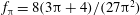 $f_{{\rm\pi}}=8(3{\rm\pi}+4)/(27{\rm\pi}^{2})$
for the drag coefficient, which differs by less than
$f_{{\rm\pi}}=8(3{\rm\pi}+4)/(27{\rm\pi}^{2})$
for the drag coefficient, which differs by less than
 $20\,\%$
from the exact value
$20\,\%$
from the exact value
 $f=1/2$
(cf. (2.1)). The torque
$f=1/2$
(cf. (2.1)). The torque
 $M_{{\rm\pi}}$
associated with half of the drag force (3.10),
$M_{{\rm\pi}}$
associated with half of the drag force (3.10),
 $$\begin{eqnarray}M_{{\rm\pi}}={\textstyle \frac{16}{3}}{\it\mu}_{1}RUa\left[1+O\left(\cot ({\it\Theta}/2)\right)\right]={\textstyle \frac{16}{3}}{\it\mu}_{1}a^{2}U\sin {\it\Theta}[1+O(\cot ({\it\Theta}/2))],\end{eqnarray}$$
follows from the fact that the pressure is homogeneous on the disk surface (cf. (50) in Tanzosh & Stone Reference Tanzosh and Stone1996), and therefore does not contribute to the torque. The direction of positive torque is defined in figure 1(b).
4 Discussion
In figure 3, we compare the result (2.21) and its first-order part (2.2) to experimental and theoretical drag coefficient values from the literature. The numerical solution to the full flow problem by Zabarankin (Reference Zabarankin2007) may serve as a reference. The point where
 ${\it\Theta}=0$
corresponds to the case of two touching spheres, to which the result
${\it\Theta}=0$
corresponds to the case of two touching spheres, to which the result
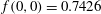 $f(0,0)=0.7426$
by Jeffrey & Onishi (Reference Jeffrey and Onishi1984), coinciding with the value by Zabarankin (Reference Zabarankin2007), applies. As can be seen, the first-order result (2.2) already agrees well with the reference data. The inclusion of the
$f(0,0)=0.7426$
by Jeffrey & Onishi (Reference Jeffrey and Onishi1984), coinciding with the value by Zabarankin (Reference Zabarankin2007), applies. As can be seen, the first-order result (2.2) already agrees well with the reference data. The inclusion of the
 $\cos ^{2}{\it\Theta}$
-term, resulting in (2.21), leads to a significantly better agreement between the asymptotic model and the numerical solution. With a maximum error in the drag coefficient
$\cos ^{2}{\it\Theta}$
-term, resulting in (2.21), leads to a significantly better agreement between the asymptotic model and the numerical solution. With a maximum error in the drag coefficient
 $f$
of less than 0.02 (3 %), the quadratic expression may even be applied to the full range of contact angles between
$f$
of less than 0.02 (3 %), the quadratic expression may even be applied to the full range of contact angles between
 $0^{\circ }$
and
$0^{\circ }$
and
 $90^{\circ }$
. Although the region where
$90^{\circ }$
. Although the region where
 $90^{\circ }<{\it\Theta}<180^{\circ }$
lacks experimental and numerical reference data, the qualitative behaviour of the drag coefficient in that region may be discussed. The drag coefficient is expected to approach zero when the contact angle approaches
$90^{\circ }<{\it\Theta}<180^{\circ }$
lacks experimental and numerical reference data, the qualitative behaviour of the drag coefficient in that region may be discussed. The drag coefficient is expected to approach zero when the contact angle approaches
 $180^{\circ }$
, a behaviour which is not reproduced by (2.21), but by the result (3.11). Therefore, a transition region between the two expressions (2.21) and (3.11) exists. Numerical values of the drag coefficient in that region can be approximated by an interpolation formula, e.g.
$180^{\circ }$
, a behaviour which is not reproduced by (2.21), but by the result (3.11). Therefore, a transition region between the two expressions (2.21) and (3.11) exists. Numerical values of the drag coefficient in that region can be approximated by an interpolation formula, e.g.
 $$\begin{eqnarray}f({\it\Theta},0)\approx 2\left(1-\frac{{\it\Theta}}{{\rm\pi}}\right)f_{{\rm\pi}/2}+2\left(\frac{{\it\Theta}}{{\rm\pi}}-\frac{1}{2}\right)f_{{\rm\pi}},\quad \frac{{\rm\pi}}{2}<{\it\Theta}<{\rm\pi},\end{eqnarray}$$
as plotted in figure 3.
5 Conclusions
With (2.21), (3.11) and (2.22), we have developed explicit expressions for the drag and diffusion coefficients of a spherical particle attached to the interface between two immiscible fluids for the case of a small viscosity ratio between the two phases. The relations account for the dependence on the contact angle between the two fluids and the solid surface. Following from the assumption on the viscosity ratio, the drag and diffusion coefficients of a pair of fused spheres moving perpendicular to their line-of-centres has been found simultaneously. This approach had been designed to cover contact angles near
 $90^{\circ }$
. The extension to contact angles near
$90^{\circ }$
. The extension to contact angles near
 $180^{\circ }$
has been provided by considering a perturbation about a disk shape. A comparison between the two models and reference data has shown that the model (2.21) can be applied to the entire range of contact angles below
$180^{\circ }$
has been provided by considering a perturbation about a disk shape. A comparison between the two models and reference data has shown that the model (2.21) can be applied to the entire range of contact angles below
 $90^{\circ }$
with high accuracy. In conjunction with the model (3.11) applicable at large contact angles and with the interpolation formula (4.1), the drag and diffusion coefficients for contact angles between
$90^{\circ }$
with high accuracy. In conjunction with the model (3.11) applicable at large contact angles and with the interpolation formula (4.1), the drag and diffusion coefficients for contact angles between
 $0^{\circ }$
and
$0^{\circ }$
and
 $180^{\circ }$
can be accurately described. The method, originally developed by Brenner (Reference Brenner1964), can be applied to any particle shape resulting from a small geometric modification of another particle shape with a known flow field. Finally, we note that the extension of our analyses to the systems with phases of comparable viscosity might not be straightforward unless the interface passes through the particle’s plane of symmetry (i.e.
$180^{\circ }$
can be accurately described. The method, originally developed by Brenner (Reference Brenner1964), can be applied to any particle shape resulting from a small geometric modification of another particle shape with a known flow field. Finally, we note that the extension of our analyses to the systems with phases of comparable viscosity might not be straightforward unless the interface passes through the particle’s plane of symmetry (i.e.
 ${\it\Theta}={\rm\pi}/2$
).
${\it\Theta}={\rm\pi}/2$
).

Figure 3. Comparison of the models (2.2) and (2.21) with experimental and theoretical drag coefficient values taken from the literature. The limit of contact angles close to
 $180^{\circ }$
, (3.11), is shown as a dashed curve. In the experiments by Petkov et al. (Reference Petkov, Denkov, Danov, Velev, Aust and Durst1995), an air–water interface with a very small viscosity ratio,
$180^{\circ }$
, (3.11), is shown as a dashed curve. In the experiments by Petkov et al. (Reference Petkov, Denkov, Danov, Velev, Aust and Durst1995), an air–water interface with a very small viscosity ratio,
 ${\it\mu}_{2}/{\it\mu}_{1}\approx 0.02$
, was studied. The remaining curves are valid under the assumption
${\it\mu}_{2}/{\it\mu}_{1}\approx 0.02$
, was studied. The remaining curves are valid under the assumption
 ${\it\mu}_{2}/{\it\mu}_{1}=0$
.
${\it\mu}_{2}/{\it\mu}_{1}=0$
.
While the relevance of this work for cases with contact angles below or close to
 $90^{\circ }$
seems evident, particles with very large contact angles appear to be quite exotic. However, in the past few years methods have been described to fabricate superhydrophobic particles, and corresponding applications have been sketched (Larmour, Saunders & Bell Reference Larmour, Saunders and Bell2008; Zhang et al.
Reference Zhang, Wu, Wang, Long, Zhao and Xu2012). A prominent feature of superhydrophobic particles is their high mobility on water surfaces, for which the results of this article provide a mathematical description.
$90^{\circ }$
seems evident, particles with very large contact angles appear to be quite exotic. However, in the past few years methods have been described to fabricate superhydrophobic particles, and corresponding applications have been sketched (Larmour, Saunders & Bell Reference Larmour, Saunders and Bell2008; Zhang et al.
Reference Zhang, Wu, Wang, Long, Zhao and Xu2012). A prominent feature of superhydrophobic particles is their high mobility on water surfaces, for which the results of this article provide a mathematical description.
Acknowledgements
A.D. and S.H. gratefully acknowledge financial support by the German Research Foundation through grant no. HA 2696/25-1. H.M. acknowledges support from DOE grant DE-FG02-88ER25053 and from NSF grant DMR-0844115 and the Institute for Complex Adaptive Matter. H.A.S. acknowledges support from NSF grant CBET-1234500.
Supplementary material
Supplementary material is available at http://dx.doi.org/10.1017/jfm.2016.41.


