


1. Introduction
The laminar to turbulent transition in pipe flow is one of the most important problems in fluid mechanics (Eckhardt et al. Reference Eckhardt, Schneider, Hof and Westerweel2007), initiated by O. Reynolds in 1887 (Reynolds Reference Reynolds1883). The flow in a pipe is characterised by a non-dimensional parameter, the Reynolds number defined as  ${Re}=U R /\nu$ where
  $U$ is the flow velocity,
  $R$ the diameter of the pipe and
  $\nu$ the dynamic viscosity of the fluid. The question about the critical Reynolds number
  ${Re}_{c}$ is the following: At which Reynolds number does the flow in a pipe become turbulent from laminar (and vice versa)? Though its apparent simplicity, answering this question was not straightforward due to a number of technical reasons (see Eckhardt (Reference Eckhardt2009) for a historical review of the critical Reynolds number). After the 2000s, a localised turbulent state (figure 1) called ‘puff’ (Wygnanski & Champagne Reference Wygnanski and Champagne1973) created by a local perturbation to laminar flows has been studied in detail. The puff shows a sudden decay or splitting after a stochastic waiting time, following a memoryless exponential distribution (Hof, Westerweel, Schneider & Eckhardt Reference Hof, Westerweel, Schneider and Eckhardt2006; Hof, de Lozar, Kuik & Westerweel Reference Hof, de Lozar, Kuik and Westerweel2008; de Lozar & Hof Reference de Lozar and Hof2009; Avila, Willis & Hof Reference Avila, Willis and Hof2010; Kuik, Poelma & Westerweel Reference Kuik, Poelma and Westerweel2010). These studies culminated in the estimation of the critical Reynolds number in 2011 (Avila et al. Reference Avila, Moxey, de Lozar, Avila, Barkley and Hof2011), where
  ${Re}_{c}$ was determined as the
  ${Re}$ at which the two typical times of the decay and splitting become equal. The obtained
  ${Re}_{c}$ was approximately 2040 (Avila et al. Reference Avila, Moxey, de Lozar, Avila, Barkley and Hof2011).

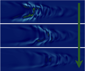
Figure 1. A pipe flow simulation with a diameter  $D$ and length
  $L$, containing a single turbulent puff, is considered. In the figure, the velocity component perpendicular to the figure is visualised using a colourmap. We perform many pipe flow simulations during a certain time interval, where the initial conditions are slightly different from each other (so that the dynamics are independent after a relaxation time). We consider the sum of all the durations of the simulations (where the initial relaxation intervals and the intervals after the puff decays are subtracted). We denote this total duration by
  $T$ and also the total number of decay events observed in all the simulations by
  $n_{d}$. From this pair of quantities, we estimate the typical decay time
  $\tau _{d}$ as
  $T/n_{d}$ and its error bars by using Bayesian inference as detailed in the main text. See also appendix A for more details of the simulation architecture.
The critical Reynolds number was determined in laboratory experiments using long pipes. In direct numerical simulations (DNS) of the Navier–Stokes equations, the observation of the critical Reynolds number has not yet been achieved because of too high computational costs. The current state of the art is to measure decay events up to  $Re=1900$ and splitting events down to
  $2100$ (Avila et al. Reference Avila, Moxey, de Lozar, Avila, Barkley and Hof2011). There are several important benefits in measuring these decay and splitting events in DNS. First, in experiments, unknown background noise that affects the results could exist. See, for example, Eckhardt (Reference Eckhardt2009) for a history of the struggle to determine the upper critical Reynolds number due to small background fluctuations. In DNS on the other hand, we know all the origins of the artificial noise, such as insufficient mesh sizes or periodic boundary effects, which can be easily controlled. Second, the quantities that are measurable in experiments are limited. For example, to determine the critical Reynolds number, a double-exponential fitting curve was heuristically used (Hof et al. Reference Hof, Westerweel, Schneider and Eckhardt2006, Reference Hof, de Lozar, Kuik and Westerweel2008; Avila et al. Reference Avila, Moxey, de Lozar, Avila, Barkley and Hof2011). The origin of this double-exponential law was discussed using the extreme value theory (Goldenfeld, Guttenberg & Gioia Reference Goldenfeld, Guttenberg and Gioia2010; Goldenfeld & Shih Reference Goldenfeld and Shih2017), where Goldenfeld et al. conjectured that the cumulative distribution function (CDF) of maximum kinetic energy fluctuations has a certain form. Measurements of this probability function are out of reach in experiments, but can be achieved in DNS.
In this article by using high performance computing resources described in the acknowledgments, we study the statistics of turbulence decay in pipe flows with DNS. We perform more than 1000 independent pipe flow simulations in parallel (see appendix A) and determine the decay time up to  $Re=2000$. Especially, our aim is to investigate if the CDF of a maximum turbulence intensity is described by the double-exponential Gumbel distribution as conjectured by (Goldenfeld et al. Reference Goldenfeld, Guttenberg and Gioia2010; Goldenfeld & Shih Reference Goldenfeld and Shih2017) to derive the double-exponential law.
2. Set-up
We consider three-dimensional pipe flows (with pipe length  $L$ and pipe diameter
  $D$) where the boundaries are periodic for the
  $z$-axis and no-slip along the pipe (figure 1). The mean flow speed in the
  $z$ direction is denoted by
  $U_{b}$ and we use the basic unit of length and time as
  $D$ and
  $D/U_{b}$ throughout this paper. The velocity field is denoted by
  $\boldsymbol{u}(\boldsymbol{r},t)$ and we simulate its evolution by solving the Navier–Stokes equations using an open source code (openpipeflow Willis (Reference Willis2017)) whose validity has been widely tested in many works (see appendix A for the simulation detail). We simulate pipe flows for the Reynolds numbers below the critical value
  ${Re}<{Re}_{c}\sim 2040$, where the flows tend to be laminar. We start the simulations with initial conditions where localised turbulence, i.e. a turbulent puff, exists (see appendix A for more details). If the Reynolds number is not too small (say,
  ${Re}>1850$), localised turbulent dynamics are sustained (figure 1). It quickly forgets their initial conditions and eventually decays after the stochastic time
  $t$, following an exponential distribution function (Hof et al. Reference Hof, Westerweel, Schneider and Eckhardt2006, Reference Hof, de Lozar, Kuik and Westerweel2008; de Lozar & Hof Reference de Lozar and Hof2009; Avila et al. Reference Avila, Willis and Hof2010; Kuik et al. Reference Kuik, Poelma and Westerweel2010):
  $p_{d}(t)=(1/\tau _{d})\exp (-t/\tau _{d})$, where
  $\tau _{d}$ is the typical decay time. This time scale
  $\tau _{d}$ is our target.
3. Results
3.1. Measurements of  $\tau _{d}$

To measure  $\tau _{d}$, we perform many pipe flow simulations and measure the total time
  $T$ of all the simulations (ignoring initial relaxation intervals) and the number of decay events
  $n_{d}$ that we observe during all the simulations. The typical decay time
  $\tau _{d}$ can be estimated as
  $T/n_{d}.$ This estimate converges to the true value as we observe more decay events. Since we observe only a few decay events when the Reynolds number is large (as shown in table 1), it is then important to calculate accurately the statistical errors of this estimate. To this end, we use Bayesian inference as detailed as follows: since the decay time is distributed exponentially (Hof et al. Reference Hof, Westerweel, Schneider and Eckhardt2006, Reference Hof, de Lozar, Kuik and Westerweel2008; de Lozar & Hof Reference de Lozar and Hof2009; Avila et al. Reference Avila, Willis and Hof2010; Kuik et al. Reference Kuik, Poelma and Westerweel2010), the probability of observing
  $n_{d}$ decay events during a time interval
  $T$ follows the Poisson distribution
 \begin{equation} p_{poisson}(n_{d})=\frac{\textrm{e}^{-\lambda_{d} T}}{n_{d}!} \left (\lambda_{d} T \right )^{n_{d}},\end{equation}
where  $\lambda _{d}\equiv 1/\tau _{d}$. To derive a probability distribution of the rate
  $\lambda _{d}$ from this Poisson distribution, we use Bayes’ rule. It allows us to construct a posterior probability distribution
  $p_{posterior}(\lambda _{d}\,|\,n_d)$, i.e. the probability distribution of the parameter
  $\lambda _{d}$ for a given observed data
  $n_d$, as follows:
 \begin{equation} P_{posterior}(\lambda_{d}\,|\,n_d) \propto p_{poisson}(n_{d}) Q_{prior}(\lambda_{d}). \end{equation}
Here  $Q_{prior}(\lambda _{d})$ is a prior probability distribution that represents the initial guess of the parameter distribution. In our case, as we do not know the probability of
  $\lambda _{d}$ a priori, we use a Jeffreys prior (an uninformative prior) defined as the square root of the determinant of the Fisher information (Box & Tiao Reference Box and Tiao2011),
  $Q_{prior}(\lambda _{d}) \propto 1/\sqrt {\lambda _{d}}$. With this posterior distribution
  $P_{posterior}(\lambda _{d}\,|\,n_d)$, we define the error bars using 95 % confidence intervals: we define 2.5th percentile
  $\lambda _{{d}}^{2.5}$ and 97.5th percentile
  $\lambda _{{d}}^{97.5}$ as the values of
  $\lambda _{d}$ at which the cumulative posterior probability distribution takes 0.025 and 0.975, respectively, i.e.
  $\int _{0}^{\lambda _{{d}}^{2.5}} \,\textrm {d}\lambda _{d}\, P_{posterior}(\lambda _{d}\,|\,n_d) = 0.025$ and
  $\int _{0}^{\lambda _{{d}}^{97.5}} \,\textrm {d}\lambda _{d}\, P_{posterior}(\lambda _{d}|n_d) = 0.975$. Using these percentiles, the 95 % confidence interval is then defined as
  $\lambda _{{d}}^{2.5}<\lambda _{d}<\lambda _{{d}}^{97.5}$.
Table 1. The number of threads  $M$, the simulation time interval for each thread (
 $K$ in wall time and
  $K_{conv}$ in convective units
  $D/U_{b}$), the number of decaying events
  $n_{d}$ (for all threads during the simulation interval
  $K$) and the total simulation interval
  $T$ in convective units (for all threads during the simulation time
  $K$, excluding the initial relaxation time). Here
  $K_{conv}$ slightly fluctuates depending on the thread, so the average value over all the threads is used (i.e.
  $K_{conv} \equiv T / M$). Note also that
  $K_{conv}$ do not include the initial relaxation time, while
  $K$ does. For the simulations, we used two cluster machines: CINES OCCIGEN and TGCC Joliot Curie KNL Irene, where
  $({Re}, L) = (1900, 50), (1925, 50), (1950, 50), (1900, 100), (1925, 100), (1950, 100), (2040, 50)$ used CINES OCCIGEN, while
  $({Re}, L) = (1975, 50), (2000, 50)$ used TGCC-IreneKNL and
  $({Re}, L) = (1975, 100)$ used the combined data obtained from both machines.

We show in figure 2 the obtained  $\tau _{d}$ for different pipe lengths
  $L=50D, L=100D$ (red circles and blue squares, respectively) together with the experimentally fitted double-exponential (yellow dashed) curve used in Avila et al. (Reference Avila, Moxey, de Lozar, Avila, Barkley and Hof2011). For the Reynolds number up to 1900 (which has been studied so far using DNS),
  $\tau _{d}$ does not depend on the pipe length, and the results for both pipe lengths agree very well with the experimental data. However, as the Reynolds number increases, we observe that the results for
  $L=100D$ deviate from those for
  $L=50D$ and for the experiments. In DNS, periodic boundary conditions introduce confinement effects on the puff: an insufficient pipe length in DNS prevents the puff from fully developing as it would in an infinite pipe. In the range of the pipe length we studied, this confinement facilitates decay events (i.e. as the pipe length increases, the average decay time also increases). Note that the experimental results are of the same order as the DNS result for
  $L=50D$, even though the pipe lengths used for the experiments were much longer (Avila et al. Reference Avila, Moxey, de Lozar, Avila, Barkley and Hof2011). Further numerical studies are necessary to understand the convergence of the decay time as the pipe length increases. Below we discuss the derivation of the double-exponential formula for each fixed
  $L=50D$ and
  $L=100D$.

Figure 2. The typical decay time  $\tau _{d}$ of turbulent puff in pipe flows obtained from DNS (red dots for
  $L=50D$ and blue squared for
  $L=100D$). Double-exponential curves fitted to experiments (Avila et al. Reference Avila, Moxey, de Lozar, Avila, Barkley and Hof2011) plotted as a yellow dashed line, and our theoretical lines (3.10) are also plotted as red and blue solid lines. The error bars show 95 % confidence interval (see the main text for the definition). The inset shows the same data but with
  $\log \tau _{d}$.
3.2. Statistical property of the maximum turbulence intensity
For the Reynolds number dependence of the time scale  $\tau _{d}$, a double-exponential fitting curve
  $\exp [ \exp (\alpha {Re} + \beta ) ]$ (with fitting parameters
  $\alpha ,\beta$) was heuristically used (Avila et al. Reference Avila, Moxey, de Lozar, Avila, Barkley and Hof2011). Although this function can fit well to the experimentally observed time scale
  $\tau _{d}$, the origin of this double exponential form is still conjectural. In the conjecture made by Goldenfeld et al. (Reference Goldenfeld, Guttenberg and Gioia2010), they assumed that the maximum of the kinetic energy fluctuations over the pipe is distributed double-exponentially (the Gumbel distribution function) due to the extreme value theory (Fisher & Tippett Reference Fisher and Tippett1928; Gumbel Reference Gumbel1935). When this maximum goes below a certain threshold, turbulence decays. Assuming the linear dependence on
  $Re$ of the parameters in the Gumbel distribution function, they thus derived the double-exponential increase of the time scale
  $\tau _{d}$. Mathematically proving the validity of the extreme value theory and the linear scaling of the fitting parameters seems impossible, thus verifications in experiments or numerical simulations are needed. In laboratory experiments, the verification of this extreme value theory is not easy, as obtaining the maximum of a velocity field within a tiny turbulent puff is a non-trivial procedure. In this respect, numerical simulations have a strong advantage, because velocity fields are precisely tractable and the maximum of the fields is well-defined.
To this goal, we characterise the intensity of turbulence by using the squared  $z$-component of vorticity
  $H(\boldsymbol{r},t)=(\boldsymbol {\nabla } \times \boldsymbol{u})_z^2$. (Note that there are other quantities that can characterise the turbulence intensity, such as the kinetic energy fluctuations – see appendix B for the result obtained using this latter quantity.) We then consider the maximum value of this turbulence intensity over the pipe (maximum turbulence intensity),
 \begin{equation} h^{max}(t) = \mathop{max}\limits_{\boldsymbol{r}}H(\boldsymbol{r},t). \end{equation}
Once this quantity goes below a certain threshold  $h_{\textrm {th}}$,
  $h^{max}(t)$ monotonically decreases, leading to a quick exponential decay of the puff (i.e. the puff dynamics shows transient chaos (Hof et al. Reference Hof, de Lozar, Kuik and Westerweel2008; Barkley Reference Barkley2011)). See figure 3(a) for a decaying trajectory of
  $h^{max}(t)$. In order to measure the CDF of
  $h^{max}(t)$ in our numerical simulations, we save the value of
  $h^{max}(t)$ for every fixed time interval
  $\delta t$ (we stop saving
  $h^{max}(t)$ once a value of
  $h^{max}(t)$ satisfying
  $h^{max}(t) < h_{\textrm {th}}$ is saved). We denote by
  $(h^{max}(t_i))_{i=1}^{N}$ the data obtained from all the simulations with the number of saving points
  $N$. By using this data, we then define a CDF
  $P(h)$ as the probability that
  $h^{max}(t)$ takes a value less than or equal to
  $h$
$h$
 \begin{equation} P(h) = \sum_{i=1}^{N}\frac{\varTheta (h - h^{max}(t_i))}{N} \end{equation}
with a Heaviside step function  $\varTheta (h)$. Note that the number of decay events
  $n_{d}$ is equal to
  $NP(h_{\textrm {th}})$ because
  $n_{d} = \sum _{i=1}^{N} \varTheta (h_{\textrm {th}} - h^{max}(t_i)) = NP(h_{\textrm {th}})$. This indicates that the decay time
  $\tau _{d}\equiv (N\delta t)/n_{d}$ is expressed as (Nemoto & Alexakis Reference Nemoto and Alexakis2018)
 \begin{equation} \tau_{d} = \frac{\delta t}{P(h_{\textrm{th}})}, \end{equation}
when  $N$ is sufficiently large. We set
  $h_{\textrm {th}}=0.1$ throughout this article. Precisely, the threshold value
  $h_{\textrm {th}}$ should be defined as the value below which puffs always decay monotonically, but above which puffs have a certain probability to grow up and survive, even if this probability is very small. In reality, it is not easy to determine this precise value
  $h_{\textrm {th}}^*$ from numerical simulations. Fortunately, the magnitude of the errors (due to an underestimation of
  $h_{\textrm {th}} < h^*_{\textrm {th}}$) does not depend on the Reynolds number and it is proportional to
  $\log (h^*_{\textrm {th}}/h_{\textrm {th}})$ because of the exponential decay of puffs when
  $h_{\textrm {th}}$ is very small. When we consider
  ${Re}$ close to its critical value, these errors are negligible as
  $\tau _{d}$ increases super-exponentially.

Figure 3. (a) A trajectory of the maximum turbulence intensity  $h^{max}(t)$ for
  $L=50D$ and
  $Re=1900$, where the puff decays when
  $t\simeq 1000$. We set
  $h_{\textrm {th}}=0.1$, below which the maximum turbulence intensity always monotonically decreases (i.e. puffs always decay). This threshold line is shown as a black dotted line. (b) The CDF of the maximum turbulence intensity
  $P(h)$ (3.4) divided by its minimum value
  $P(h_{\textrm {th}})$, obtained from numerical simulations (solid coloured lines). The measurement interval
  $\delta t$ is set to 1/4. The pipe length is set to
  $L=50D$. (For
  $L=100D$, similar results are obtained.) Below a certain value
  $h_{x}$, the function
  $P(h)/P(h_{\textrm {th}})$ becomes independent of Reynolds number. This
  $h_{x}$ is shown as a vertical red dotted line, being around 6.5 for
  $L=50D$ and 7.5 for
  $L=100D$. For
  $h>h_{x}$,
  $P(h)$ is well approximated by the Gumbel function
  $P_{Re}(h)$ (3.6): we fit
  $P_{Re}(h)/P(h_{\textrm {th}})$ to
  $P(h)/P(h_{\textrm {th}})$ for
  $h>h_{x}$ and show them as coloured dashed lines. See table 2 for the fitting parameters
  $\gamma$ and
  $h_0$ used in this figure. Note that the value of
  $1/P(h_{\textrm {th}})$ is represented as the length of the double-headed arrow (for
  $Re=1975$). From this figure, we estimate
  $\varPi (h_{x}) \equiv P(h_{x})/P(h_{\textrm {th}}) \simeq 158.8$ for
  $L=50D$ and 219.2 for
  $L=100D$.


We measure this CDF  $P(h)$ in DNS, rescale it by the threshold probability
  $P(h_{\textrm {th}})$, and plot it in figure 3(b). When
  $h$ is smaller than a certain value
  $h_{x} \ (>h_{\textrm {th}})$, the overlap of
  $P(h)/P(h_{\textrm {th}})$ between different Reynolds numbers is observed, i.e.
  $P(h)/P(h_{\textrm {th}}) \simeq \varPi (h)$ for
  $h < h_{x}$ with a
  $Re$-independent function
  $\varPi (h)$. Note that
  $h_{x} \simeq 6.5$ for
  $L=50D$ and
  $h_{x} \simeq 7.5$ for
  $L=100D$ from figure 3(b). From this tendency, we expect that
  $h_{x}$ increases gradually as
  $L$ increases, which eventually converges to a certain value. This convergence can be studied in numerical simulations with the Reynolds number that is relatively far away from the critical value (e.g.
  $Re = 1900$) – this is an interesting topic for future study. When
  $h^{max}(t)$ is smaller than
  $h_{x}$, dynamics are in a metastable state where the puff is hovering between death and life (see figure 3a). This overlap indicates that the dynamics in this metastable state are independent of (or less sensitive to) the change of the Reynolds number. On the other hand, when
  $h$ is greater than this value, we find that
  $P(h)$ is well-described by the Gumbel distribution function
  $P_{Re}$,
 \begin{equation} P_{Re}(h) \equiv \exp[-\exp(-\gamma (h-h_0))], \end{equation}
where  $\gamma$,
  $h_0$ are fitting parameters depending on
  $Re$. In summary, we have confirmed that the scaled probability
  $P(h)/P(h_{\textrm {th}})$ is well approximated as
 \begin{equation} \frac{P(h)}{P(h_{\textrm{th}})} \simeq \begin{cases} \varPi (h) & h \leq h_{x} \\ P_{Re}(h)/ P(h_{\textrm{th}}) & h > h_{x}. \end{cases} \end{equation}
 Based on this observation, the double-exponential increase of the mean decay time is justified as follows. From the continuity condition of (3.7) at  $h=h_{x}$, we get
  $\varPi (h_{x}) = P_{Re}(h_{x})/ P(h_{\textrm {th}})$. Using the relation (3.5) that connects the decay time
  $\tau _{d}$ and
  $P(h_{\textrm {th}})$, we then derive
 \begin{equation} \tau_{d} = \delta t / P(h_{\textrm{th}}) = \delta t \varPi(h_{x}) \exp[ \exp\left ( \gamma (h_0-h_{x}) \right )]. \end{equation}
In the right-hand side of this expression, the  $Re$-dependence only comes from
  $\gamma$ and
  $h_0$, because
  $h_{x}$ does not depend on
  ${Re}$ (at least in the range of
  ${Re}$ we consider). In order to study the
  ${Re}$-dependence on
  $\gamma$ and
  $h_0$, we next plot these quantities as a function of
  $Re$ in figure 4(a). The figure indicates that, within the examined range, these parameters depend linearly on
  $Re$. Especially, we can see that the slope of the linear fitting curve for
  $\gamma$ is much smaller than that for
  $h_0$, which means we can approximate
  $\gamma h_0$ as a linear function of
  $Re$. We thus get
 \begin{equation} \gamma (h_0-h_{x}) \simeq a \, {Re} + b \end{equation}
with coefficients  $a$ and
  $b$. In figure 4(b), we confirm this linear approximation by plotting the left-hand side of (3.9) as a function of
  ${Re}$. We also determine the coefficients
  $a$ and
  $b$ from this figure, and summarise them in the caption of figure 4(b). Finally, using (3.9) in (3.8), we derive the double-exponential formula
 \begin{equation} \tau_{d} \simeq \delta t \varPi(h_{x}) \exp[\exp\left ( a \, {Re} + b \right ) ]. \end{equation}
Using  $\delta t = 1/4$ and the values of
  $\varPi (h_{x})$ measured in figure 3(b) (together with
  $a,b$ obtained in figure 4b), we plot this double exponential formula in figure 2 as red and blue solid lines. These theoretical lines are consistent with the direct measurements (red circles and blue squares). Note that the parameters
  $\gamma , h_0$ are determined from the measurements up to
  $Re=1975$ for
  $L=50D$ and up to
  $Re=1950$ for
  $L=100D$. But the obtained curves agree with the direct measurements for
  $Re=2000$ with
  $L=50D$ and for
  $Re=1975$ with
  $L=100D$. This observation indicates that our method can be used to infer statistical properties in higher Reynolds numbers from the data obtained in lower Reynolds numbers.

Figure 4. (a) The fitting parameters  $\gamma$ and
  $h_0$ in the Gumbel function (3.6), used in figure 3(b), as a function of
  $Re$. Red circles, yellow diamonds, blue squares and green triangles correspond to
  $h_0$ with
  $L=50D$,
  $\gamma$ with
  $L=50D$,
  $h_0$ with
  $L=100D$ and
  $\gamma$ with
  $L=100D$, respectively. To plot them together in the same panel, we divide each
  $\gamma ({Re})$ and
  $h_0({Re})$ by
  $\gamma (1900)$ and
  $h_0(1900)$. They show linear dependence on Reynolds number: the solid and dashed straight lines are the linear fit. See table 3 for the slopes and intercepts of these linear lines. Note that the slopes of the fitting lines for
  $h_0/h_0(1900)$ are much larger than those for
  $\gamma /\gamma (1900)$. (b)
  $\gamma ({Re}) [h_0({Re})-h_{x}]$ as a function of
  ${Re}$, where
  $\gamma ({Re})$ and
  $h_0({Re})$ use the same values in panel (a), and
  $h_{x}=6.5$ for
  $L=50D$ and
  $h_{x}=7.5$ for
  $L=100D$. We find a linear dependence
  $\gamma ({Re}) [h_0({Re})-h_{x}] = a \, {Re} + b$ (3.9). Here
  $a$ and
  $b$ are determined as
  $a=0.00895442$,
  $b=-15.6087$ for
  $L=50D$ and
  $a=0.0105166$,
  $b=-18.6222$ for
  $L=100D$.
Table 3. Fitting parameters determined in figure 4(a). A linear function  $S \, {Re} + I$ with a slope
  $S$ and an intercept
  $I$ is fitted to
  $\bar \gamma (Re) \equiv \gamma (Re) / \gamma (1900)$ and
  $\bar h_0 ({Re}) \equiv h_0({Re})/h_0(1900)$. See table 2 for the values of
  $\gamma (1900), h_0(1900)$.

3.3. Relevance with the extreme value theory
Our formula (3.10) is the product of (i) the double exponential term  $\exp [ \exp ( a {Re} + b )]$ and (ii) the constant term (independent of
  $Re$)
$Re$)  $\varPi (h_x) \delta t$. The first double-exponential term is attributed to the probability of the event in which
  $h_{max}$ of a fully developed puff is weakened to
  $h_{x}$. After this event, the weakened puff undergoes metastable dynamics as shown in the time series in figure 3(a). These metastable dynamics are known as edge states (de Lozar et al. Reference de Lozar, Mellibovsky, Avila and Hof2012). On the other hand, the second term corresponds to the average time for these metastable puffs to completely decay. In the original conjecture in Goldenfeld et al. (Reference Goldenfeld, Guttenberg and Gioia2010) and Goldenfeld & Shih (Reference Goldenfeld and Shih2017), this second term was not considered. However, when the Reynolds number is close to its critical value, we expect that the double-exponential term becomes dominant, so that their argument is still reasonable.
As seen in the previous subsection, the first term (i) was derived from the Gumbel distribution function introduced in the approximation (3.7). The validity of this Gumbel distribution is where the extreme value theory could be relevant: the Fisher–Tippett–Gnedenko (FTG) theorem ensures that the CDF of the maximum value of a set of independent stochastic variables becomes either the Gumbel distribution function (3.6), Fréchet distribution function or Weibull distribution function (Fisher & Tippett Reference Fisher and Tippett1928; Gumbel Reference Gumbel1935). Inspired by this theorem, Goldenfeld et al conjectured in Goldenfeld et al. (Reference Goldenfeld, Guttenberg and Gioia2010) and Goldenfeld & Shih (Reference Goldenfeld and Shih2017) that the Gumbel distribution function described the maximum turbulence intensity. In this work, we confirmed that this conjecture was approximately satisfied.
3.4. Close-up of the Gumbel distribution approximation
The approximation of the CDF using the Gumbel distribution (3.7) was the key to the derivation of the double-exponential formula (3.10). Interestingly, in a detailed look at figure 3(b), we detect small errors in this approximation (for  $h$ larger than 20), though the errors are too small to affect the derivation of (3.10). In general, approximations are better in CDFs than in probability distribution functions (p.d.f.s) defined as the derivative of CDFs, because taking the derivative magnifies the errors. In this subsection, we thus investigate the corresponding p.d.f. in order to understand the origin of these errors. This is important for future studies to apply the same formulation to different problems or to investigate the same problem with a higher Reynolds number.
We study the p.d.f. of the maximum turbulence intensity  $\textrm {d} P(h)/\textrm {d} h$, by plotting it together with the corresponding Gumbel probability distribution
  $\textrm {d} P_{Re}(h)/\textrm {d} h$ in figure 5(a). We can detect clear discrepancies between the p.d.f. and the Gumbel distribution function for
  $h>20$, to which we attribute two reasons. First, the condition of the FTG theorem may not be exactly satisfied. For example, the turbulence-intensify field is not spatially independent, whereas the independence is required for the FTG theorem to be applied. (The original FTG theorem requires the variables to be independent but this condition can be weakened (Charras-Garrido & Lezaud Reference Charras-Garrido and Lezaud2013). It is anyway difficult to justify it with our turbulence intensify a priori.) Second, assuming the FTG theorem is applicable, the Gumbel distribution function may not be the correct one: it may be either the Fréchet distribution function or the Weibull distribution function describing the maximum turbulence intensify fluctuations. We can easily rule out the Weibull distribution, as it is for random variables with an upper bound (which is not true in our turbulence-intensity field). The Fréchet distribution is defined as
 \begin{equation} P_{Re}^{F}(h) \equiv \exp[-\kappa (h-\eta) ^{-\zeta} ],\end{equation}
where  $\kappa , \eta , \zeta$ are parameters. A characteristic of the Fréchet distribution is the power law decay of the logarithm of the CDF (cf. the exponential decay in the case of the Gumbel distribution). The FTG theorem states that, when the distribution function of each variable (the turbulence intensity field for each position in our problem) decays in power laws, the maximum among these variables is described by the Fréchet distribution with
  $\zeta$ equal to the decay exponent of each variable (cf. when the distribution function of each variable decays exponentially, the maximum among these variables is described by the Gumbel distribution). We fit the Fréchet distribution to our p.d.f. of the maximum turbulence intensity
  $\textrm {d} P(h)/\textrm {d} h$ by tuning the three parameters
  $\kappa , \eta , \zeta$. Surprisingly, the agreement in the Fréchet distribution is far better than the Gumbel distribution function, as shown in figure 5(b). The p.d.f.,
  $\textrm {d} P(h)/\textrm {d} h$, clearly shows a presence of the power law decay for large turbulence intensity that can be explained by the Fréchet distribution, but not by the Gumbel distribution. (The p.d.f. of the Gumbel distribution is
  $\gamma \exp [ - \gamma (h-h_0) - \textrm {e}^{-\gamma (h-h_0)} ]$ that decays exponentially when
  $h$ is large, while the p.d.f. of the Fréchet distribution is
  $\kappa \zeta (h-\eta ) ^{-1-\zeta } \exp [ - \kappa (h-\eta ) ^{-\zeta }]$ that decays in power law when
  $h$ is large. In figure 5, we can clearly see that
  $dP(h)/dh$ decays slower than exponential (and decays in a power law).)

Figure 5. Probability distribution function of the maximum turbulence intensity  $\textrm {d} P(h)/\textrm {d} h$ (where
  $P(h)$ is the CDF defined in (3.4)). The Gumbel distribution function (3.6) and the Fréchet distribution function (3.11) are fitted to these curves and plotted, respectively, in panel (a) and in panel (b) as dashed lines.
Nevertheless, as long as we consider the decay time, the errors in the Gumbel distribution approximation in p.d.f. are not important, because the CDF, which plays a key role in the derivation of the decay time (for example, as seen from (3.5),  $\tau _{d}$ is directly related to
  $1/P(h_{\textrm {th}})$ (as indicated as the double-headed arrow in figure 3b), which is hardly affected by tiny deviations between the Gumbel distribution and the CDF) is hardly affected by these errors. Indeed, replacing the Gumbel distribution function by the Fréchet distribution function in the argument of § 3.2 still leads to the same result (3.10) (see appendix C). But in the future, when we study the same problem with higher precisions (more statistics), or when we study the problem in higher Reynolds numbers, we could possibly detect the deviations from the double-exponential formula (3.10). In that case, using the Fréchet distribution function for more accurate analysis will be interesting.
4. Conclusion
In this paper, using a large number of DNS, we measure the decay time of turbulent puff in pipe flows up to  $Re=2000$. In DNS, periodic boundary conditions are employed in the axial direction, so that the insufficient length of the pipe introduces confinement effects on puff dynamics. Our numerical simulations show that, as the length of the pipe increases (i.e. as the confinement effects disappear), the obtained decay times increase, resulting in values larger than those used in Avila et al. (Reference Avila, Moxey, de Lozar, Avila, Barkley and Hof2011) for large Reynolds numbers (that were not previously studied using DNS). We also note that the curvature of the double exponential curves between our theoretical line (3.8) and the one used in Avila et al. (Reference Avila, Moxey, de Lozar, Avila, Barkley and Hof2011) is slightly different. Indeed in the inset of figure 2,
  $\log \tau _{d}$ shows a straight line in the form used by Avila et al. (Reference Avila, Moxey, de Lozar, Avila, Barkley and Hof2011), while our theoretical expression (3.10) shows a lightly curved line. The difference between the two formulae is a constant term
  $c$ by which the double-exponential form is multiplied:
  $c \exp [ \exp [a\, {Re} + b]]$ (with parameters
  $a,b$) where
  $c = 1$ for the form used in Avila et al. (Reference Avila, Moxey, de Lozar, Avila, Barkley and Hof2011), while
  $c = \delta t \varPi (h_{x})$ for our expression (
 $\log \{ \log \{ c \exp \{ \exp [a\, {Re} + b] \} \} \} = \log [\log c +\exp [a {Re} + b] ]$, which becomes a linear function of
  ${Re}$ only when
  $c=1$). Note that the value of the constant term changes in a different time unit, which indicates that
  $c=1$ in the convective time unit (
 $D/U_{b}$) used in Avila et al. (Reference Avila, Moxey, de Lozar, Avila, Barkley and Hof2011) is an approximation.
It was conjectured in Goldenfeld et al. (Reference Goldenfeld, Guttenberg and Gioia2010) and Goldenfeld & Shih (Reference Goldenfeld and Shih2017) that the double-exponential formula of the mean decay time could be derived using the Gumbel distribution function of maximum kinetic energy fluctuations based on the extreme value theory. We measure the CDF of the maximum turbulence intensity (3.3) and show that the function is indeed approximately described by the Gumbel distribution function (3.6), demonstrating that their conjecture is reasonable, in the range of the Reynolds number between 1900 and 2000. In § 3.4, we also study the corresponding p.d.f., and find that another extreme value distribution, the Fréchet distribution (3.11), fits better than the Gumbel distribution, indicating the presence of the power law decay in the distribution of the turbulence intensity field. This finding implies that the double-exponential formula of the decay time could be merely an approximation. It will be interesting to study the same problem with more detailed statistics or with a higher Reynolds number, as the true expression of the mean decay time could be possibly discovered using the same approach developed in this article.
Our approach will be also important for the future study in different problems of turbulence, where the extreme events trigger transitions. For example, a similar turbulence-decay problem has been studied in a different geometry (channel flows) in Shimizu, Kanazawa & Kawahara (Reference Shimizu, Kanazawa and Kawahara2019), where they observed the agreement between the probability distribution of a turbulence intensity and the Gumbel distribution in a linear-scale plot. It would be interesting to ask if the Fréchet distribution fits better in their case as well with more detailed statistics. Furthermore, turbulent transitions between two- and three-dimensional dynamics have been long studied (Smith, Chasnov & Waleffe Reference Smith, Chasnov and Waleffe1996; Celani, Musacchio & Vincenzi Reference Celani, Musacchio and Vincenzi2010; Benavides & Alexakis Reference Benavides and Alexakis2017; Musacchio & Boffetta Reference Musacchio and Boffetta2017; Alexakis & Biferale Reference Alexakis and Biferale2018), where a super-exponential increase of the transition time was observed in thin-layer turbulent condensates (van Kan, Nemoto & Alexakis Reference van Kan, Nemoto and Alexakis2019). This super-exponential increase could be also studied using the extreme value theory.
Studying these super exponential problems in DNS is computationally demanding. A brute force approach using a large number of DNS is efficient as proved in this work. But exploiting so-called rare event sampling methods could be also helpful. Such sampling methods include instanton methods based on Freidlin–Wentzell theory (Chernykh & Stepanov Reference Chernykh and Stepanov2001; Heymann & Vanden-Eijnden Reference Heymann and Vanden-Eijnden2008; Grafke, Grauer & Schäfer Reference Grafke, Grauer and Schäfer2015a; Grafke et al. Reference Grafke, Grauer, Schäfer and Vanden-Eijnden2015b; Grigorio et al. Reference Grigorio, Bouchet, Pereira and Chevillard2017) as well as splitting methods that simulate several copies in parallel (Allen, Warren & ten Wolde Reference Allen, Warren and ten Wolde2005; Giardinà, Kurchan & Peliti Reference Giardinà, Kurchan and Peliti2006; Cérou & Guyader Reference Cérou and Guyader2007; Tailleur & Kurchan Reference Tailleur and Kurchan2007; Nemoto et al. Reference Nemoto, Bouchet, Jack and Lecomte2016; Teo et al. Reference Teo, Mayne, Schulten and Lelièvre2016; Lestang et al. Reference Lestang, Ragone, Bréhier, Herbert and Bouchet2018; Bouchet, Rolland & Simonnet Reference Bouchet, Rolland and Simonnet2019). These methods have been successfully applied to many high-dimensional chaotic dynamics and proved invaluable.
Acknowledgements
The authors thank D. Barkley and L. Tuckerman for fruitful discussions and comments.
Funding
This work was granted access to the HPC resources of CINES/TGCC under the allocation 2018-A0042A10457 made by GENCI (a total of three million hours) and of MesoPSL financed by the Region Ile de France and the project Equip@Meso (reference ANR-10-EQPX-29-01) of the program Investissements d'Avenir supervised by the Agence Nationale pour la Recherche.
Declaration of interests
The authors report no conflict of interest.
Appendix A. Simulation detail
We used an open source code openpipeflow (Willis Reference Willis2017), which simulates flows in a cylindrical domain by solving the Navier–Stokes equations. Below are the summary of the parameters and the settings we used.
(i) For azimuthal and longitudinal directions of the pipe, the spectral decomposition is used to evaluate the derivatives, for which we use 24 variables for the azimuthal direction and 384 variables (for
$L=50D$) or 768 variables (for $L=100D$) for the longitudinal directions. For the radial direction, a finite-element method is used, for which the radial space is divided into 64 points using Chebyshev polynomials.(ii) The code can solve the Navier–Stokes equations under two conditions: fixed flux conditions and fixed pressure conditions. In the present study we used the fixed flux condition for the simulations.
(iii) For the time step, the algorithm uses a second-order predictor–corrector scheme with automatic time-step control with courant number 0.5.
(iv) We define that a puff decays when
$h^{max}<0.1$ is satisfied. We never observed that a puff regenerates once $h^{max}<0.1$ is observed.(v) To prepare initial velocity fields, we use a configuration where a single steady puff already exists. We added a small Gaussian noise to this configuration, and simulate it during a time interval 50 or 100. These time intervals are our initial relaxation time – see figure 6 for how the trajectories of
$h^{max}$ with different initial conditions deviate with each other. From the figure, we confirm that $t=20\sim 30$ for ${Re} = 1900$ and less for ${Re} > 1900$ could be large enough to make the dynamics independent, so that our initial relaxation interval (50 or 100) is reasonable. We also checked that both initial relaxation intervals (50 and 100) show consistent (almost the same) results for ${Re}\geq 1900$. (When an initial relaxation interval is sufficiently large, the time at which we observe the decay of puff (measured from the initial relaxation time) is distributed as the memoryless exponential probability. This memoryless distribution leads to the Poisson distribution for the number of decays, as we used in the main text (3.1). Increasing further the initial relaxation time simply results in reducing the amount of data we gathered.)(vi) We set the time interval of saving data
$\delta t$ to be 1/4 (in units of $D/U_{b}$) for the simulations in figure 3(b). Note that $P(h_{\textrm {th}}) = 1/N$ (from (3.4)), where $N$ is the number of saving points. Since $N$ is inversely proportional to the saving interval $\delta t$, we find that multiplying $\delta t$ by an arbitrary factor $c$ simply changes the probability $P(h_{\textrm {th}})$ to $P(h_{\textrm {th}}) c$. The decay time $\tau _{d}$ is then independent of $\delta t$, because $\tau _{d} = \delta t / P(h_{\textrm {th}})$ (3.5). Furthermore, in our theoretical expression of $\tau _{d}$ in (3.8), the change of $\delta t$ is compensated by the change of $\varPi (h_{x})$ without affecting the double exponential term. This can be seen from a numerical example of $P(h)$ in figure 7 – changing $\delta t$ only alters the functional shape of $P(h)$ close to $h_{\textrm {th}}$, which leaves $P(h)$ for $h\geq h_{x}$ unchanged. Multiplying $\delta t$ by an arbitrary factor $c$ thus changes $\varPi (h_{x})(\equiv P(h_{x})/P(h_{\textrm {th}}))$ to $\varPi (h_{x}) /c$, which compensates the change of $\delta t$ in (3.8).


Figure 6. Plots of 30 different  $h^{max}$ trajectories starting from different initial conditions for
  ${Re} = 1900$ and
  $L=50D$. We add a small Gaussian noise to a configuration containing a single puff, to generate different initial conditions. After the Lyapunov time, the effect of the small noise becomes exponentially important and make the dynamics with slightly different initial conditions be independent. Here we see that
  $t=20 \sim 30$ is large enough to make the dynamics independent. For the Reynolds numbers higher than 1900, we expect that the Lyapunov time is much smaller, as the dynamics is more chaotic.

Figure 7. The CDF  $P(h)$ for different saving times
  $\delta t$ for
  ${Re}=1900$,
  $L=50D$. We observe that changing
  $\delta t$ only affects the functional shape of
  $P(h)$ close to
  $h_{\textrm {th}}$ without changing
  $P(h)$ for
  $h\geq h_{x}$. In this figure,
  $P(h_{\textrm {th}})|_{\delta t =1/4} = 0.0001113$ and
  $P(h_{\textrm {th}})|_{\delta t =1/2} = 0.0002226$, so we get
  $2 P(h_{\textrm {th}})|_{\delta t =1/4} = P(h_{\textrm {th}})|_{\delta t =1/2}$. This relation is generally true as explained in the last bullet point of appendix A: multiplying
  $\delta t$ by an arbitrary factor results in multiplying
  $P(h_{\textrm {th}})$ by the same factor. This means that the average decay time
  $\tau _{d} (= \delta t / P(h_{\textrm {th}}))$ (3.5) is independent of the value of
  $\delta t$.
A.1. Parallelisation
Although the open source code openpipeflow has an option to use multiple threads for a single pipe flow simulation, relying on it when we use a considerably larger number of threads would not be efficient. What we are interested in are the statistical properties of the decay events of the puff, which can be accumulated in independent simulations. Instead of parallelising a single pipe flow simulation, we thus simulate many pipe flows in an embarrassingly parallel way, where each thread is used to simulate a single pipe flow. Here we explain the detail of the architecture of this parallelisation.
As shown in figure 8, we perform  $M$ independent pipe flow simulations. Each pipe flow simulation is allocated to a single thread, thus
  $M$ threads are required for these simulations. The initial conditions of these simulations are slightly different from each other, so that the simulations become independent after an initial relaxation interval. During these simulations, when a puff decays in a thread, we immediately launch another pipe flow simulation in that thread using a new initial condition (that contains a developed puff but different from the other initial conditions that have been already used). All threads are thus always occupied. We continue these simulations for a computational time interval
  $K$ (or
  $K_{conv}$ in convective time units). We summarise in table 1 the values of
  $M$ and
  $K$ we use, as well as the number of decay events
  $n_{d}$ we observe.

Figure 8. We simultaneously simulate  $M$ pipe flow simulations with different initial conditions in
  $M$ threads, where each pipe flow simulation is allocated to a single thread. When a decay of puff is observed in a thread, we immediately launch another pipe flow simulation in that thread with a different initial condition. The simulations continue during a time interval
  $K$. The values of these
  $M$ and
  $K$ are summarised in table 1.
Appendix B. CDF of the maximum kinetic energy fluctuations
We define the kinetic energy fluctuations  $E$ as the kinetic energy of the flow fields without the contribution of the laminar flow
  $\boldsymbol{u}_{lam}$:
  $E(\boldsymbol{r}, t)= [ \boldsymbol{u} (\boldsymbol{r}, t) - \boldsymbol{u}_{lam} ]^2$. Similarly to
  $h^{max}(t)$, we define the maximum value of this kinetic energy fluctuations over the pipe as
 \begin{equation} \textrm{e}^{max}(t) = \mathop{max}\limits_{\boldsymbol{r}} E(\boldsymbol{r}, t). \end{equation}
The CDF of this  $\textrm {e}^{max}(t)$ is defined in the same way as in (3.4), denoted by
  $P(e)$. We measure
  $P(e)$ in numerical simulations and show it in figure 9. It shows qualitatively similar structures as those in figure 4(b), namely the function is composed of the two parts: (i) the part that can be approximately described by the Gumbel distribution and (ii) the relatively flat part that is related to the dynamics of a metastable puff.

Figure 9. The CDF of the maximum kinetic energy fluctuations  $\textrm {e}^{max}(t)$ defined in (B1), obtained from numerical simulations (solid line) with
  ${Re}=1900$,
  $L=50D$. The Gumbel distribution function (3.6) is fitted to this data and shown as a yellow dashed line. The parameters in the fitting curve are determined as
  $\gamma = 26.27, h_0 = 0.2073$.
Appendix C. Using the Fréchet distribution function still leads to (3.10)
The approximation errors from the Gumbel distribution in the p.d.f. do not affect the double-exponential formula (3.10), as long as the errors are well-hidden in the corresponding CDF. This indicates that, even if we use the Fréchet distribution to approximate  $P(h)$, this will still leads to the same double exponential formula (3.10), at least as an approximation. We demonstrate it in this appendix.
We fit the Fréchet distribution function (3.11) to the CDF of the maximum turbulence intensity  $P(h)$ (3.4) and plot it in figure 10(a). The figure indicates that
  $P(h)$ is approximated as
 \begin{equation} \frac{P(h)}{P(h_{\textrm{th}})} \simeq \begin{cases} \varPi (h) & h \leq h_{x} \\ P_{Re}^{F}(h)/ P(h_{\textrm{th}}) & h > h_{x} \end{cases} \end{equation}
with an  $Re$-independent function
  $\varPi (h)$ (cf. (3.7) using the Gumbel distribution function). We observe slightly larger discrepancies in this approximation close to
  $h=h_{x}$ than in (3.7) (yet, we observe better agreement for
  $h>20$ – see the explanation in § 3.4). For this technical reason,
  $h_{x}$ is defined as the value that makes
  $P_{Re}^{F}(h_{x})/ P(h_{\textrm {th}})$ the same for all
  $Re$ we study. These values are provided in the caption of figure 10(a) together with the values of
  $\varPi (h_{x}) (\equiv P_{Re}^{F}(h_{x})/ P(h_{\textrm {th}}) )$. Following the same argument below (3.6), we then derive
 \begin{equation} \tau_{d} = \delta t \varPi(h_{x}) \exp[ \kappa (h_{x}-\eta) ^{-\zeta} ]. \end{equation}
We next plot  $\log [\kappa (h_{x} - \eta )^{-\zeta } ]$ in figure 10(b) as a function of
  $Re$, which shows a linear relationship,
 \begin{equation} \log [ \kappa (h_{x}-\eta) ^{-\zeta}] \simeq \tilde a\, {Re} + \tilde b. \end{equation}
Here the values of the parameters  $\tilde a, \tilde b$ are provided in the caption of figure 10(b). We thus again arrive at
 \begin{equation} \tau_{d} \simeq \delta t \varPi(h_{x}) \exp[ \exp ( \tilde a\, {Re} + \tilde b)],\end{equation}
which is the same as (3.10). Though the parameters in this expression ( $\varPi (h_x), \tilde a, \tilde b$) are slightly different from the ones in (3.10), this (C4) still produces very similar lines to the ones plotted in figure 2 as shown in figure 10(c).

Figure 10. (a) The CDF of the maximum turbulence intensity  $P(h)/P(h_{\textrm {th}})$ in solid lines, together with the fitted Fréchet distribution function in dashed lines (cf. the same CDF with the fitted Gumbel distribution function in figure 3a). The pipe length is
  $L=50D$ in this figure and a similar graph is obtained with
  $L=100D$. The values of
  $h_{x}$,
  $\varPi (h_{x}) (\equiv P_{Re}^{F}(h_{x})/ P(h_{\textrm {th}}))$ are (
 $8, 108.2$) for
  $L=50D$ and (
 $8.5, 130.8$) for
  $L=100D$, respectively. (b) Here
  $\log [\kappa (h_{x} - \eta )^{-\zeta }]$ as a function of
  $Re$, where
  $\kappa , \eta , \zeta$ are the fitting parameters of the Fréchet distribution function (3.11) determined in panel (a) for each
  $Re$. A straight line (C3) is fitted to each plot and shown as a red solid line (
 $L=50D$) and a blue solid line (
 $L=100D$). The fitting parameters
  $(\tilde a,\tilde b)$ are determined as
  $(-14.1817, 0.00825304)$ for
  $L=50D$ and
  $(-17.0837, 0.00976833)$ for
  $L=100D$. (c) The mean decay time
  $\tau _{d}$ obtained from DNS are plotted as red dots (
 $L=50D$) and blue squares (
 $L=100D$). This is the same plot as figure 2 except for the formula derived from the Fréchet distribution (C4), which is plotted as a red solid line (
 $L=50D$) and a blue solid line (
 $L=100D$).


