


1 Introduction
In hydraulic fracturing, specially engineered suspensions are pumped at high pressure and rate into the reservoir, causing a propagating fracture to open. When the pressure is released the fracture is held open by packed grains of solid proppant (typically natural angular sand) that are left behind. This method increases the hydraulic conductivity and consequently enhances well production. At various stages in the process, streamwise dispersion of proppant can be important, e.g. tip screen-out and spreading of the pad. Streamwise dispersion is also critically important in a recent process variation called the channel fracturing technique (CFT) (Gillard et al. Reference Gillard, Medvedev, Pena, Medvedev, Penacorada and d’Huteau2010). The key concept here is to substitute the usual continuous stream of proppant slurry that fills the fracture with discrete pillars of proppant that hold open the fracture. The increased hydraulic conductivity of the clear channels between the pillars has the overall effect of a significant increase in fracture conductivity. To produce the pillar configuration in the fracture, slugs of proppant are interspersed with clear fracturing fluid at the wellhead. Eventually it is expected that these slugs enter the fracture, and remain distinct for sufficiently long for the fracture to close on them. Proper design of this pumping technique obviously requires an understanding of dispersion mechanisms, both in the well and along the fracture. One proposed method for controlling dispersion is via the frac fluid rheology and in particular use of a yield stress fluid, which may also enhance the transport capacity. In this study we aim to develop a model framework for studying these flows within the fracture, with a particular emphasis on streamwise dispersion and shear-thinning yield stress frac fluids.
By design, our study cuts across many related areas. There are many examples of using the Hele-Shaw approach to model fracture flows (e.g. Pearson Reference Pearson1994; Hammond Reference Hammond1995; Mobbs & Hammond Reference Mobbs and Hammond2001; Lakhtychkin, Vinogradov and Eskin Reference Lakhtychkin, Vinogradov and Eskin2011; Boronin & Osiptsov Reference Boronin and Osiptsov2014; Boronin, Osiptsov & Desroches Reference Boronin, Osiptsov and Desroches2015), wherein the assumption is made that the velocity field and gradients can be scaled differentially, according to the fracture aspect ratio. This allows the neglect of the inertial terms under the assumption that the bulk flow Reynolds number,
 $Re$
, multiplied by a small width-to-length ratio, is vanishingly small. On the experimental front, there are also experimental studies in Hele-Shaw cell geometries on viscous fingering (e.g. Buka, Kertesz & Vicsek Reference Buka, Kertesz and Vicsek1986; Buka & Palffy-Muhoray Reference Buka and Palffy-Muhoray1987; Lemaire et al.
Reference Lemaire, Levitz, Daccord and Van Damme1991; Lindner, Coussot & Bonn Reference Lindner, Coussot and Bonn2000; Lindner et al.
Reference Lindner, Bonn, Poire, Amar and Meunier2002; Makino et al.
Reference Makino, Kawaguchi, Aoyama and Kato2002) and on fracturing flows (e.g. Lyon & Leal Reference Lyon and Leal.1998; Liu, Gadde & Sharma Reference Liu, Gadde and Sharma2007). In real fractures and under realistic process conditions, geometric and inertial effects may become significant and there is a significant literature on improving the Hele-Shaw approach. Low-
$Re$
, multiplied by a small width-to-length ratio, is vanishingly small. On the experimental front, there are also experimental studies in Hele-Shaw cell geometries on viscous fingering (e.g. Buka, Kertesz & Vicsek Reference Buka, Kertesz and Vicsek1986; Buka & Palffy-Muhoray Reference Buka and Palffy-Muhoray1987; Lemaire et al.
Reference Lemaire, Levitz, Daccord and Van Damme1991; Lindner, Coussot & Bonn Reference Lindner, Coussot and Bonn2000; Lindner et al.
Reference Lindner, Bonn, Poire, Amar and Meunier2002; Makino et al.
Reference Makino, Kawaguchi, Aoyama and Kato2002) and on fracturing flows (e.g. Lyon & Leal Reference Lyon and Leal.1998; Liu, Gadde & Sharma Reference Liu, Gadde and Sharma2007). In real fractures and under realistic process conditions, geometric and inertial effects may become significant and there is a significant literature on improving the Hele-Shaw approach. Low-
 $Re$
experiments and computations through laboratory-produced fractures or computer-generated fractures have shown that reasonable corrections can be made for roughness and tortuosity at zero
$Re$
experiments and computations through laboratory-produced fractures or computer-generated fractures have shown that reasonable corrections can be made for roughness and tortuosity at zero
 $Re$
(e.g. Patir & Cheng Reference Patir and Cheng1978; Brown Reference Brown1987; Zimmerman, Kumar & Bodvarsson Reference Zimmerman, Kumar and Bodvarsson1991). These studies typically correct the usual (Newtonian) cubic flow law via definition of an appropriate hydraulic gap width, proposing corrections that depend on dimensionless geometric ratios such as the standard deviation to mean gap width, wavelength to mean gap width, etc.
$Re$
(e.g. Patir & Cheng Reference Patir and Cheng1978; Brown Reference Brown1987; Zimmerman, Kumar & Bodvarsson Reference Zimmerman, Kumar and Bodvarsson1991). These studies typically correct the usual (Newtonian) cubic flow law via definition of an appropriate hydraulic gap width, proposing corrections that depend on dimensionless geometric ratios such as the standard deviation to mean gap width, wavelength to mean gap width, etc.
Some of these flow laws extend to non-zero
 $Re$
(e.g. Hasegawa & Izuchi Reference Hasegawa and Izuchi1983). Apart from via simulation, it is often hard to decouple purely geometric effects from inertial effects in studying the flows through fractures. Thus, for example, Yeo, De Freitas & Zimmerman (Reference Yeo, De Freitas and Zimmerman1998) constructed artificial sandstone fractures and compared the results of flow tests with numerical simulations based on the Reynolds equation, reporting 20–25 % discrepancies for
$Re$
(e.g. Hasegawa & Izuchi Reference Hasegawa and Izuchi1983). Apart from via simulation, it is often hard to decouple purely geometric effects from inertial effects in studying the flows through fractures. Thus, for example, Yeo, De Freitas & Zimmerman (Reference Yeo, De Freitas and Zimmerman1998) constructed artificial sandstone fractures and compared the results of flow tests with numerical simulations based on the Reynolds equation, reporting 20–25 % discrepancies for
 $18<Re<60$
. Following the use of the hydraulic gap width from Hasegawa & Izuchi (Reference Hasegawa and Izuchi1983), the error was reduced by around a third. However, it is notable that significant errors persist at smaller
$18<Re<60$
. Following the use of the hydraulic gap width from Hasegawa & Izuchi (Reference Hasegawa and Izuchi1983), the error was reduced by around a third. However, it is notable that significant errors persist at smaller
 $Re$
than might be considered from a strict scaling analysis. There are also classical inertial corrections such as the Forchheimer correction (used in porous media flows) and the Ergun equations (used in packed beds).
$Re$
than might be considered from a strict scaling analysis. There are also classical inertial corrections such as the Forchheimer correction (used in porous media flows) and the Ergun equations (used in packed beds).
There have been long-standing attempts to model non-Newtonian effects in porous media – see e.g. the fine early review of Savins (Reference Savins1969) – but less specifically directed at yield stress fluids. Typically the end result is a specification of a non-Darcy (or nonlinear filtration) closure law relating superficial velocity to pressure gradients. In the case of yield stress fluids, these are generally of limiting pressure gradient type (e.g. Sultanov Reference Sultanov1960; Entov Reference Entov1967). Included in these studies and of relevance to fracture flows are some detailed two-dimensional (2D) studies: along wavy walled channels (Balhoff & Thompson Reference Balhoff and Thompson2004; Frigaard & Ryan Reference Frigaard and Ryan2004; Putz, Frigaard & Martinez Reference Putz, Frigaard and Martinez2009; Roustaei & Frigaard Reference Roustaei and Frigaard2013), through bed/fibre-type geometries (Bleyer & Coussot Reference Bleyer and Coussot2014; Shahsavari & McKinley Reference Shahsavari and McKinley2016), or other geometric variants (Roustaei, Gosselin & Frigaard Reference Roustaei, Gosselin and Frigaard2015; Roustaei et al. Reference Roustaei, Chevalier, Talon and Frigaard2016). There is also some limited study of inertial effects Roustaei & Frigaard (Reference Roustaei and Frigaard2015). In summary, these studies show that the simplistic picture of a plane Poiseuille flow with a rigid central plug is quickly destroyed by streamwise geometric variation, that new non-Darcy effects emerge via static fouling of deep wall undulations or roughness, but that suitable flow laws and limiting pressure gradient closures can be derived for specific classes of geometry.
In considering flows of yield stress fluid suspensions, we need to consider additional complexities: the frac fluid is now strongly shear thinning and, apart from a generic rheological description, process conditions can have a significant impact on the local conditions felt by particles. These conditions and effects are analysed later in this paper (§ 2.2), but to pre-empt, we find that fracture flows of yield stress fluids are unusual in allowing for a massive variation in local strain rates and effective viscosity. The consequence is that for many typical fracture flows the particle dynamics ranges from Stokesian in the fracture centre to significantly inertial close to the fracture walls. The local rheological behaviour of yield stress fluid suspensions in the Stokesian regime has recently been characterized (at least approximately) by Ovarlez, Bertrand & Rodts (Reference Ovarlez, Bertrand and Rodts2006), Chateau, Ovarlez & Luu Trung (Reference Chateau, Ovarlez and Luu Trung2008), Mahaut et al. (Reference Mahaut, Chateau, Coussot and Ovarlez2008), Coussot et al. (Reference Coussot, Tocquer, Lanos and Ovarlez2009), Vu, Ovarlez & Chateau (Reference Vu, Ovarlez and Chateau2010), Ovarlez et al. (Reference Ovarlez, Bertrand, Coussot and Chateau2012), Dagois-Bohy et al. (Reference Dagois-Bohy, Hormozi, Guazzelli and Pouliquen2015) and Ovarlez et al. (Reference Ovarlez, Mahaut, Deboeuf, Lenoir, Hormozi and Chateau.2015). We utilize these results below.
In particulate flows, the particle distribution results from hydrodynamics and multi-body interactions of the particles. In a non-homogeneous shear flow of Newtonian suspensions, it is observed that particles migrate from high- to low-shear-rate regions (Leighton & Acrivos Reference Leighton and Acrivos1987; Phillips et al. Reference Phillips, Armstrong, Brown, Graham and Abbott1992). This has been modelled phenomenologically by attributing shear-induced diffusive migration to a combination of collisional Brownian motion and viscosity variation effects. These components have measured experimentally for Newtonian suspensions by Gadala-Maria & Acrivos (Reference Gadala-Maria and Acrivos1980), Chapman (Reference Chapman1990), Phillips et al. (Reference Phillips, Armstrong, Brown, Graham and Abbott1992), Hampton et al. (Reference Hampton, Mammoli, Graham, Tetlow and Altobelli1997), Lyon & Leal (Reference Lyon and Leal.1998) and Snook, Butler & Guazzelli (Reference Snook, Butler and Guazzelli2016). A different approach is the suspension balance model (SBM), which is a hybrid theoretical–phenomenological approach in which particle migration is modelled through normal stress gradients in the particle phase. The various constants and multipliers in this approach are determined from experimental measurements and numerical simulations (e.g. Morris & Boulay Reference Morris and Boulay1999). Although there are still unanswered questions and ongoing debate on the nature of particle stress in Newtonian suspensions (e.g. Lhuillier Reference Lhuillier2009; Nott, Guazzelli & Pouliquen Reference Nott, Guazzelli and Pouliquen2011; Guazzelli & Morris Reference Guazzelli and Morris2012; Brady Reference Brady2015), numerous experimental and computational studies have been conducted that support and advance this approach (e.g. Chapman Reference Chapman1990; Phillips et al. Reference Phillips, Armstrong, Brown, Graham and Abbott1992; Merhi et al. Reference Merhi, Lemaire, Bossis and Moukalled2005; Morris Reference Morris2009; Dbouk, Lobry & Lemaire Reference Dbouk, Lobry and Lemaire2013).
The above solids dispersion models are largely restricted to Stokesian regimes and Newtonian fluids. In the fracturing context, geometric, inertial and rheological complexities are present. Neglecting the particles, there is a growing literature on dispersion in fractures (e.g. Drazer & Koplik Reference Drazer and Koplik2000, Reference Drazer and Koplik2002; Auradou et al.
Reference Auradou, Drazer, Hulin and Koplik2005, Reference Auradou, Drazer, Boschan, Hulin and Koplik2006). As with porous media dispersivities, there is considerable anisotropy due to the flow direction and fracture geometry. More recent studies have considered the effects of shear-thinning rheology on tracer dispersion Boschan et al. (Reference Boschan, Auradou, Ippolito, Chertcoff and Hulin2007), Auradou et al. (Reference Auradou, Boschan, Chertcoff, Gabbanelli, Hulin and Ippolito2008), Boschan et al. (Reference Boschan, Ippolito, Chertcoff, Auradou, Talon and Hulin2008, Reference Boschan, Auradou, Ippolito, Chertcoff and Hulin2009). One of the main features of these studies and others that focus purely on fluid flow (e.g. Skjetne, Hansen & Gudmondson Reference Skjetne, Hansen and Gudmondson1999) is that at moderate
 $Re$
the flow tends to channel through a (smoothed) central part of the fracture, leaving significant parts of the fracture with near-zero velocity, whereas creeping flows tend to fill the fracture. Similar effects were found with yield stress fluids by Roustaei & Frigaard (Reference Roustaei and Frigaard2015) and Roustaei et al. (Reference Roustaei, Gosselin and Frigaard2015). These features can have a significant effect on dispersion. It appears that there is relatively little work concerned with suspensions directly in this context.
$Re$
the flow tends to channel through a (smoothed) central part of the fracture, leaving significant parts of the fracture with near-zero velocity, whereas creeping flows tend to fill the fracture. Similar effects were found with yield stress fluids by Roustaei & Frigaard (Reference Roustaei and Frigaard2015) and Roustaei et al. (Reference Roustaei, Gosselin and Frigaard2015). These features can have a significant effect on dispersion. It appears that there is relatively little work concerned with suspensions directly in this context.
The main novel contributions of our study are as follows. Firstly, we carry out an order-of-magnitude analysis of proppant transport along typical hydraulic fractures using viscous fluids (shear thinning and yield stress), specifically focusing on the macroscale flow and the particle scale. We include recent rheological models for yield stress suspensions, in which the presence of particles increases local strain rates, thus reducing local effective viscosity. Through our analysis we show that typical suspensions in hydraulic fracturing flows exhibit a transition from Stokesian to inertial regimes, on the particle scale, as we move across the fracture width (§ 2.2). Secondly, we develop a two-phase continuum framework for modelling fracturing flows, based on the SBM of Nott & Brady (Reference Nott and Brady1994). Owing to the particle-scale behaviour and the nature of the fluids, we extend the SBM approach in two directions: (i) we incorporate the shear-thinning yield stress rheology of the fluid; (ii) we incorporate inertial/unsteady ranges of particle behaviour using an order-of-magnitude analysis of the different flow regimes. We also incorporate in our model closure expressions for the various forces experienced by the particles, but only so far as to give an estimate of the size of these effects (§ 2.4). Thirdly, we reduce the overall model using scaling arguments to arrive at two tractable systems of reduced equations that model these flows, depending on whether or not the macroscale effects of inertia are negligible, which depends on the usual lubrication modelling criterion of
 $Re\unicode[STIX]{x1D6FF}_{t}\ll 1$
(
$Re\unicode[STIX]{x1D6FF}_{t}\ll 1$
(
 $Re$
being the Reynolds number and
$Re$
being the Reynolds number and
 $\unicode[STIX]{x1D6FF}_{t}$
a suitable aspect ratio). Both systems (see § 3) result in 2D models of the in-plane flow variables and distribution of proppant. Finally in § 4 we explore a simplification of the lubrication model (
$\unicode[STIX]{x1D6FF}_{t}$
a suitable aspect ratio). Both systems (see § 3) result in 2D models of the in-plane flow variables and distribution of proppant. Finally in § 4 we explore a simplification of the lubrication model (
 $Re\unicode[STIX]{x1D6FF}_{t}\ll 1$
) that allows a one-dimensional (1D) model of proppant dispersion along a streamline of the width-averaged flow. We find that to leading-order dispersion is advective not diffusive, and use this model to study pulsed proppant distributions such as in the CFT. In addition, we obtain the transverse distributions of the solid volume fraction and velocity profiles as well as their evolutions along the flow part.
$Re\unicode[STIX]{x1D6FF}_{t}\ll 1$
) that allows a one-dimensional (1D) model of proppant dispersion along a streamline of the width-averaged flow. We find that to leading-order dispersion is advective not diffusive, and use this model to study pulsed proppant distributions such as in the CFT. In addition, we obtain the transverse distributions of the solid volume fraction and velocity profiles as well as their evolutions along the flow part.
2 Flow regimes in fractures
A difficulty in modelling many industrial processes is the wide range of operational regimes and parameters. From a fluid mechanics perspective, we need to understand the influence of operational parameters on the flows, defining what are typical flows and identifying the key characteristics. This is the goal here. We first discuss some general parameter ranges directly below. We then address the rheology of viscoplastic suspension flows under shear in § 2.1. Section 2.3 groups bulk fracture flows broadly into three types, each of which shows different characteristic variations in strain rate and local effective viscosity across the fracture. The consequences of this variation are discussed in § 2.3, from the perspective of regimes that the particle experiences, and this is put in the context of recent dimensional scaling studies. In summary, we build a comprehensive physical intuition of these flows before developing our continuum modelling approach in § 2.4.
2.1 Rheology
For a broad picture of the full range of complex fluids used in hydraulic fracturing, we refer the reader to the recent review of Barbati et al. (Reference Barbati, Desroches, Robisson and McKinley2016). As mentioned in the introduction, we focus on viscous frac fluids as opposed to slickwater slurries, and we target dispersive phenomena in proppant transport. Thus, shear rheology is more important than viscoelasticity for these aspects, although viscoelasticity is ever present in frac fluids. A wide range of fluids are used, according to operation and company, often with proprietary formulation, e.g. typically aqueous polymer gels (guar, hydroxypropyl guar (HPG), etc.), either linear gels or cross-linked (e.g. with borate). These fluids are quite viscous and often strongly shear thinning. A common oilfield characterization is via a power-law model, with consistency
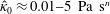 $\hat{\unicode[STIX]{x1D705}}_{0}\approx 0.01{-}5~\text{Pa}~\text{s}^{n}$
and power-law index
$\hat{\unicode[STIX]{x1D705}}_{0}\approx 0.01{-}5~\text{Pa}~\text{s}^{n}$
and power-law index
 $n\approx 0.2{-}1$
. Some fluids may have a modest yield stress,
$n\approx 0.2{-}1$
. Some fluids may have a modest yield stress,
 $\hat{\unicode[STIX]{x1D70F}}_{Y0}\approx 0{-}15~\text{Pa}$
. For a typical frac fluid based on guar, we might expect
$\hat{\unicode[STIX]{x1D70F}}_{Y0}\approx 0{-}15~\text{Pa}$
. For a typical frac fluid based on guar, we might expect
 $0.35<n<0.6$
and
$0.35<n<0.6$
and
 $0.1<\hat{\unicode[STIX]{x1D705}}_{0}<1$
 $(\text{Pa}~\text{s}^{n})$
. One also sees frac fluids with shear-thinning exponents in the 0.2–0.3 range, often with larger
$(\text{Pa}~\text{s}^{n})$
. One also sees frac fluids with shear-thinning exponents in the 0.2–0.3 range, often with larger
 $\hat{\unicode[STIX]{x1D705}}_{0}$
. Rheological parameters are not independently variable. At high shear rates the effective viscosity tends to plateau, e.g. we would not expect the effective viscosity of viscous frac fluids to fall significantly below
$\hat{\unicode[STIX]{x1D705}}_{0}$
. Rheological parameters are not independently variable. At high shear rates the effective viscosity tends to plateau, e.g. we would not expect the effective viscosity of viscous frac fluids to fall significantly below
 $0.01~\text{Pa}~\text{s}$
.
$0.01~\text{Pa}~\text{s}$
.
To incorporate the range of shear rheologies, we will assume that the effective viscosity of the pure frac fluid is modelled reasonably well as a Herschel–Bulkley fluid, with effective viscosity
 $\hat{\unicode[STIX]{x1D702}}_{f,0}(\hat{\dot{\unicode[STIX]{x1D6FE}}})$
, possibly bounded below at high shear. Ovarlez and co-workers have recently developed a general framework for shear-thinning and yield stress fluid suspensions that has been validated at least partially (see Ovarlez et al.
Reference Ovarlez, Bertrand and Rodts2006, Reference Ovarlez, Bertrand, Coussot and Chateau2012, Reference Ovarlez, Mahaut, Deboeuf, Lenoir, Hormozi and Chateau.2015; Chateau et al.
Reference Chateau, Ovarlez and Luu Trung2008; Mahaut et al.
Reference Mahaut, Chateau, Coussot and Ovarlez2008; Coussot et al.
Reference Coussot, Tocquer, Lanos and Ovarlez2009; Vu et al.
Reference Vu, Ovarlez and Chateau2010; Dagois-Bohy et al.
Reference Dagois-Bohy, Hormozi, Guazzelli and Pouliquen2015). The bulk suspension viscosity
$\hat{\unicode[STIX]{x1D702}}_{f,0}(\hat{\dot{\unicode[STIX]{x1D6FE}}})$
, possibly bounded below at high shear. Ovarlez and co-workers have recently developed a general framework for shear-thinning and yield stress fluid suspensions that has been validated at least partially (see Ovarlez et al.
Reference Ovarlez, Bertrand and Rodts2006, Reference Ovarlez, Bertrand, Coussot and Chateau2012, Reference Ovarlez, Mahaut, Deboeuf, Lenoir, Hormozi and Chateau.2015; Chateau et al.
Reference Chateau, Ovarlez and Luu Trung2008; Mahaut et al.
Reference Mahaut, Chateau, Coussot and Ovarlez2008; Coussot et al.
Reference Coussot, Tocquer, Lanos and Ovarlez2009; Vu et al.
Reference Vu, Ovarlez and Chateau2010; Dagois-Bohy et al.
Reference Dagois-Bohy, Hormozi, Guazzelli and Pouliquen2015). The bulk suspension viscosity
 $\hat{\unicode[STIX]{x1D702}}$
, is decomposed as
$\hat{\unicode[STIX]{x1D702}}$
, is decomposed as
 $$\begin{eqnarray}\hat{\unicode[STIX]{x1D702}}=\hat{\unicode[STIX]{x1D702}}_{f}\unicode[STIX]{x1D702}_{r}(\unicode[STIX]{x1D719}),\end{eqnarray}$$
where
 $\hat{\unicode[STIX]{x1D702}}_{f}$
is referred to as the liquid-phase viscosity and
$\hat{\unicode[STIX]{x1D702}}_{f}$
is referred to as the liquid-phase viscosity and
 $\unicode[STIX]{x1D702}_{r}(\unicode[STIX]{x1D719})$
is the dimensionless relative viscosity, modelled for example by the Krieger–Dougherty law
$\unicode[STIX]{x1D702}_{r}(\unicode[STIX]{x1D719})$
is the dimensionless relative viscosity, modelled for example by the Krieger–Dougherty law
 $$\begin{eqnarray}\unicode[STIX]{x1D702}_{r}(\unicode[STIX]{x1D719})=\left[1-\frac{\unicode[STIX]{x1D719}}{\unicode[STIX]{x1D719}_{m}}\right]^{-2.5\unicode[STIX]{x1D719}_{m}},\end{eqnarray}$$
or a close variant (see Maron & Pierce Reference Maron and Pierce1956; Dougherty Reference Dougherty1959; Krieger Reference Krieger1972; Quemada Reference Quemada, Casas-Vazquez and Lebon1982). Apart from conceptual simplicity, there exist generalizations of such laws to particles of different shapes, e.g. rods/fibres (see Wierenga & Philips Reference Wierenga and Philips1998). Here
 $\unicode[STIX]{x1D719}_{m}$
denotes the maximal packing fraction. The relative viscosity is further decomposed into
$\unicode[STIX]{x1D719}_{m}$
denotes the maximal packing fraction. The relative viscosity is further decomposed into
 $\unicode[STIX]{x1D702}_{r}(\unicode[STIX]{x1D719})=\unicode[STIX]{x1D702}_{p}(\unicode[STIX]{x1D719})+1$
, where
$\unicode[STIX]{x1D702}_{r}(\unicode[STIX]{x1D719})=\unicode[STIX]{x1D702}_{p}(\unicode[STIX]{x1D719})+1$
, where
 $\unicode[STIX]{x1D702}_{p}(\unicode[STIX]{x1D719})$
is called the particle-phase viscosity, satisfying
$\unicode[STIX]{x1D702}_{p}(\unicode[STIX]{x1D719})$
is called the particle-phase viscosity, satisfying
 $\unicode[STIX]{x1D702}_{p}(\unicode[STIX]{x1D719})\sim \unicode[STIX]{x1D719}$
as
$\unicode[STIX]{x1D702}_{p}(\unicode[STIX]{x1D719})\sim \unicode[STIX]{x1D719}$
as
 $\unicode[STIX]{x1D719}\rightarrow 0$
and
$\unicode[STIX]{x1D719}\rightarrow 0$
and
 $\unicode[STIX]{x1D702}_{p}(\unicode[STIX]{x1D719})\rightarrow \infty$
as
$\unicode[STIX]{x1D702}_{p}(\unicode[STIX]{x1D719})\rightarrow \infty$
as
 $\unicode[STIX]{x1D719}\rightarrow \unicode[STIX]{x1D719}_{m}$
. The combination
$\unicode[STIX]{x1D719}\rightarrow \unicode[STIX]{x1D719}_{m}$
. The combination
 $\hat{\unicode[STIX]{x1D702}}_{f}\unicode[STIX]{x1D702}_{p}(\unicode[STIX]{x1D719})$
usually appears as part of the solids-phase stress.
$\hat{\unicode[STIX]{x1D702}}_{f}\unicode[STIX]{x1D702}_{p}(\unicode[STIX]{x1D719})$
usually appears as part of the solids-phase stress.
In the liquid phase the particles act to amplify effects of a bulk shear rate imposed on the suspension, i.e. since the particles themselves do not deform. This amplification can be crudely estimated as
 $$\begin{eqnarray}\hat{\dot{\unicode[STIX]{x1D6FE}}}_{loc}=\left[\frac{\unicode[STIX]{x1D702}_{r}(\unicode[STIX]{x1D719})}{1-\unicode[STIX]{x1D719}}\right]^{1/2}\hat{\dot{\unicode[STIX]{x1D6FE}}},\end{eqnarray}$$
which is verified reasonably well by experimental results (Ovarlez et al.
Reference Ovarlez, Bertrand and Rodts2006; Mahaut et al.
Reference Mahaut, Chateau, Coussot and Ovarlez2008; Dagois-Bohy et al.
Reference Dagois-Bohy, Hormozi, Guazzelli and Pouliquen2015) and agrees with the theoretical considerations of Chateau et al. (Reference Chateau, Ovarlez and Luu Trung2008). When the strain rate
 $\hat{\dot{\unicode[STIX]{x1D6FE}}}$
is imposed on the suspension,
$\hat{\dot{\unicode[STIX]{x1D6FE}}}$
is imposed on the suspension,
 $\hat{\dot{\unicode[STIX]{x1D6FE}}}_{loc}$
is representative of that felt by the local fluid and particle, and assuming a Herschel–Bulkley type closure,
$\hat{\dot{\unicode[STIX]{x1D6FE}}}_{loc}$
is representative of that felt by the local fluid and particle, and assuming a Herschel–Bulkley type closure,
 $$\begin{eqnarray}\hat{\unicode[STIX]{x1D702}}_{f}(\hat{\dot{\unicode[STIX]{x1D6FE}}},\unicode[STIX]{x1D719})=\hat{\unicode[STIX]{x1D702}}_{f,0}(\hat{\dot{\unicode[STIX]{x1D6FE}}}_{loc}(\unicode[STIX]{x1D719}))=\hat{\unicode[STIX]{x1D705}}_{0}\left[\frac{\unicode[STIX]{x1D702}_{r}(\unicode[STIX]{x1D719})}{1-\unicode[STIX]{x1D719}}\right]^{(n-1)/2}\hat{\dot{\unicode[STIX]{x1D6FE}}}^{n-1}+\frac{\hat{\unicode[STIX]{x1D70F}}_{Y0}}{\hat{\dot{\unicode[STIX]{x1D6FE}}}}\left[\frac{\unicode[STIX]{x1D702}_{r}(\unicode[STIX]{x1D719})}{1-\unicode[STIX]{x1D719}}\right]^{-1/2}.\end{eqnarray}$$
This can be interpreted as assuming the liquid within the suspension obeys a Herschel–Bulkley type law, but with
 $\unicode[STIX]{x1D719}$
-dependent consistency and yield stress defined by
$\unicode[STIX]{x1D719}$
-dependent consistency and yield stress defined by
 $$\begin{eqnarray}\hat{\unicode[STIX]{x1D705}}=\hat{\unicode[STIX]{x1D705}}_{0}\left[\frac{\unicode[STIX]{x1D702}_{r}(\unicode[STIX]{x1D719})}{1-\unicode[STIX]{x1D719}}\right]^{(n-1)/2},\quad \hat{\unicode[STIX]{x1D70F}}_{Y}=\frac{\hat{\unicode[STIX]{x1D70F}}_{Y0}}{\left[{\displaystyle \frac{\unicode[STIX]{x1D702}_{r}(\unicode[STIX]{x1D719})}{1-\unicode[STIX]{x1D719}}}\right]^{1/2}}.\end{eqnarray}$$
When
 $\unicode[STIX]{x1D702}_{r}(\unicode[STIX]{x1D719})$
is included, the effective viscosity of the suspension increases with
$\unicode[STIX]{x1D702}_{r}(\unicode[STIX]{x1D719})$
is included, the effective viscosity of the suspension increases with
 $\unicode[STIX]{x1D719}$
, but note that the fluid viscosity (
$\unicode[STIX]{x1D719}$
, but note that the fluid viscosity (
 $\hat{\unicode[STIX]{x1D702}}_{f}$
above) decreases with
$\hat{\unicode[STIX]{x1D702}}_{f}$
above) decreases with
 $\unicode[STIX]{x1D719}$
.
$\unicode[STIX]{x1D719}$
.
2.2 Dimensional analysis
Figure 1 schematically illustrates a fracture, somewhat distant from the well. Fundamentally, this is a shear flow along a channel of varying width and orientation. We assume three characteristic lengths: width
 $\hat{D}$
(5–25 mm), length
$\hat{D}$
(5–25 mm), length
 $\hat{L}$
(100–600 m) and height
$\hat{L}$
(100–600 m) and height
 ${\hat{H}}$
(20–100 m). We assume that in-plane variations occur on a length scale
${\hat{H}}$
(20–100 m). We assume that in-plane variations occur on a length scale
 $\hat{L}_{t}\lesssim \min \{\hat{L},{\hat{H}}\}$
, where
$\hat{L}_{t}\lesssim \min \{\hat{L},{\hat{H}}\}$
, where
 $\hat{L}_{t}\gg \hat{D}$
. On a scale smaller than
$\hat{L}_{t}\gg \hat{D}$
. On a scale smaller than
 $\hat{D}$
, one might also include a roughness scale
$\hat{D}$
, one might also include a roughness scale
 $\hat{d}_{w}$
.
$\hat{d}_{w}$
.

Figure 1. Schematic of a channel-like fracture. The solid phase, i.e. proppant with volume fraction
 $\unicode[STIX]{x1D719}_{in}$
, is added at the inlet to the fracturing fluid in a cyclic fashion to produce a network of open channels.
$\unicode[STIX]{x1D719}_{in}$
, is added at the inlet to the fracturing fluid in a cyclic fashion to produce a network of open channels.
The pumping process is modelled by a representative inflow velocity
 $\hat{U} _{0}$
(
$\hat{U} _{0}$
(
 $0.1{-}3~\text{m}~\text{s}^{-1}$
), or alternatively a flow rate. Additionally we specify the inflowing proppant solids fraction
$0.1{-}3~\text{m}~\text{s}^{-1}$
), or alternatively a flow rate. Additionally we specify the inflowing proppant solids fraction
 $\unicode[STIX]{x1D719}_{in}$
, (typically 5 %–40 %). These variables will be time-varying in a complex pumping operation. As the slurry travels along the fracture, some of the frac fluid may leak off into the formation. This leads to higher solid volume fractions in the fracture. Although at times this is a significant effect, for now we focus only on transport along the fracture. Although a range of proppants may be used, common is a 20/40 mesh sand with approximately spherical particles, a representative diameter
$\unicode[STIX]{x1D719}_{in}$
, (typically 5 %–40 %). These variables will be time-varying in a complex pumping operation. As the slurry travels along the fracture, some of the frac fluid may leak off into the formation. This leads to higher solid volume fractions in the fracture. Although at times this is a significant effect, for now we focus only on transport along the fracture. Although a range of proppants may be used, common is a 20/40 mesh sand with approximately spherical particles, a representative diameter
 $\hat{d}_{p}$
in the range 0.42–0.84 mm and density
$\hat{d}_{p}$
in the range 0.42–0.84 mm and density
 $\hat{\unicode[STIX]{x1D70C}}_{s}=2650~\text{kg}~\text{m}^{-3}$
. Slurry rheology has been discussed in § 2.1. We assume a frac fluid density
$\hat{\unicode[STIX]{x1D70C}}_{s}=2650~\text{kg}~\text{m}^{-3}$
. Slurry rheology has been discussed in § 2.1. We assume a frac fluid density
 $\hat{\unicode[STIX]{x1D70C}}_{f}$
(
$\hat{\unicode[STIX]{x1D70C}}_{f}$
(
 ${\approx}1000~\text{kg}~\text{m}^{-3}$
) and a representative viscosity
${\approx}1000~\text{kg}~\text{m}^{-3}$
) and a representative viscosity
 $\hat{\unicode[STIX]{x1D707}}_{f}$
.
$\hat{\unicode[STIX]{x1D707}}_{f}$
.
Even with the simplistic description above, a minimum of 11 dimensional parameters arise, depending on three independent dimensions. Thus, we expect eight dimensionless groups (plus
 $\unicode[STIX]{x1D719}_{in}$
) to govern these flows. Five of these groups are geometric. The roughness
$\unicode[STIX]{x1D719}_{in}$
) to govern these flows. Five of these groups are geometric. The roughness
 $\unicode[STIX]{x1D6FF}_{w}=\hat{d}_{w}/\hat{D}\ll 1$
we shall neglect for simplicity. On adopting
$\unicode[STIX]{x1D6FF}_{w}=\hat{d}_{w}/\hat{D}\ll 1$
we shall neglect for simplicity. On adopting
 $\hat{D}$
and
$\hat{D}$
and
 $\hat{L}_{t}$
as natural length scales for transverse and streamwise directions, we have two groups,
$\hat{L}_{t}$
as natural length scales for transverse and streamwise directions, we have two groups,
 $L=\hat{L}/\hat{D}$
and
$L=\hat{L}/\hat{D}$
and
 $H={\hat{H}}/\hat{D}$
, that simply indicate the extent of the fracture. More relevant to the transport processes are
$H={\hat{H}}/\hat{D}$
, that simply indicate the extent of the fracture. More relevant to the transport processes are
 $\unicode[STIX]{x1D6FF}_{p}=\hat{d}_{p}/\hat{D}$
and
$\unicode[STIX]{x1D6FF}_{p}=\hat{d}_{p}/\hat{D}$
and
 $\unicode[STIX]{x1D6FF}_{t}=\hat{D}/\hat{L}_{t}$
i.e. a scaled particle diameter (ratio of particle diameter to fracture width) and the local fracture aspect ratio, respectively. Note that throughout this paper we write all dimensional quantities with a
$\unicode[STIX]{x1D6FF}_{t}=\hat{D}/\hat{L}_{t}$
i.e. a scaled particle diameter (ratio of particle diameter to fracture width) and the local fracture aspect ratio, respectively. Note that throughout this paper we write all dimensional quantities with a
 $\hat{\cdot }$
symbol and dimensionless parameters without.
$\hat{\cdot }$
symbol and dimensionless parameters without.
The remaining dimensionless groups include
 $\unicode[STIX]{x1D719}_{in}$
, the density ratio
$\unicode[STIX]{x1D719}_{in}$
, the density ratio
 $s=\hat{\unicode[STIX]{x1D70C}}_{s}/\hat{\unicode[STIX]{x1D70C}}_{f}\approx 2.65$
and two others, namely the densimetric Froude number (
$s=\hat{\unicode[STIX]{x1D70C}}_{s}/\hat{\unicode[STIX]{x1D70C}}_{f}\approx 2.65$
and two others, namely the densimetric Froude number (
 $Fr$
) and Reynolds number (
$Fr$
) and Reynolds number (
 $Re$
):
$Re$
):
 $$\begin{eqnarray}Fr=\frac{\hat{U} _{0}}{\sqrt{{\hat{g}}(s-1)\hat{D}}},\quad Re=\frac{\hat{\unicode[STIX]{x1D70C}}_{f}\hat{U} _{0}\hat{D}}{\hat{\unicode[STIX]{x1D707}}_{f}}.\end{eqnarray}$$
In characterizing the rheology, we would expect at least two dimensionless groups, e.g.
 $n$
and a Bingham number
$n$
and a Bingham number
 $B_{l}=\hat{\unicode[STIX]{x1D70F}}_{Y0}/[\hat{\unicode[STIX]{x1D705}}_{0}(6\hat{U} _{0}/\hat{D})^{n}]$
. Here,
$B_{l}=\hat{\unicode[STIX]{x1D70F}}_{Y0}/[\hat{\unicode[STIX]{x1D705}}_{0}(6\hat{U} _{0}/\hat{D})^{n}]$
. Here,
 $\hat{\unicode[STIX]{x1D707}}_{f}$
is the effective viscosity of the suspending fluid and the Bingham number
$\hat{\unicode[STIX]{x1D707}}_{f}$
is the effective viscosity of the suspending fluid and the Bingham number
 $B_{l}$
is based on the nominal laminar wall shear rate,
$B_{l}$
is based on the nominal laminar wall shear rate,
 $8\hat{U} _{0}/\hat{D}$
. Further dimensionless groups may arise in characterizing the suspension (e.g.
$8\hat{U} _{0}/\hat{D}$
. Further dimensionless groups may arise in characterizing the suspension (e.g.
 $\unicode[STIX]{x1D719}_{m}$
) and in operational parameters.
$\unicode[STIX]{x1D719}_{m}$
) and in operational parameters.
2.3 Characteristics of fracture flows
In the above two subsections we have indicated the main ranges of slurry rheologies and other dimensional parameters that arise in hydraulic fracturing. In order to model these flows effectively, we need to consider the behaviour at both the bulk scale and the particle scale.
Regarding the bulk flow, pure liquid Reynolds numbers up to a maximum of
 $(5{-}10)\times 10^{3}$
are possible, but would be reduced via the presence of particles. More typically
$(5{-}10)\times 10^{3}$
are possible, but would be reduced via the presence of particles. More typically
 $Re\sim 10^{2}$
would be common in fracture transport regimes, reducing to zero in cases of screen-out. In considering asymptotic models of flow in long thin geometries, the leading-order inertial terms would be of size
$Re\sim 10^{2}$
would be common in fracture transport regimes, reducing to zero in cases of screen-out. In considering asymptotic models of flow in long thin geometries, the leading-order inertial terms would be of size
 $\unicode[STIX]{x1D6FF}_{t}Re$
. Thus, at the outset we deduce that, while non-inertial lubrication-type models have validity in suitably straight fractures, inertia of the bulk flow is important in more complex fractures even at moderate flow rates.
$\unicode[STIX]{x1D6FF}_{t}Re$
. Thus, at the outset we deduce that, while non-inertial lubrication-type models have validity in suitably straight fractures, inertia of the bulk flow is important in more complex fractures even at moderate flow rates.
To understand the shear-rate regime with the fluids considered, note that a uniform channel flow of pure frac fluid (
 $\unicode[STIX]{x1D719}=0$
) would have a layered structure consisting of an unyielded plug flow occupying a central fraction
$\unicode[STIX]{x1D719}=0$
) would have a layered structure consisting of an unyielded plug flow occupying a central fraction
 $y_{Y}$
of the channel:
$y_{Y}$
of the channel:
 $$\begin{eqnarray}\frac{B_{l}}{y_{Y}}(1-y_{Y})\left(1-\frac{1}{n+1}y_{Y}-\frac{n}{n+1}y_{Y}^{2}\right)^{n}=\left(\frac{3(2n+1)}{n}\right)^{n}\end{eqnarray}$$
(
 $y_{Y}\in [0,1]$
is readily calculated numerically). Outside of the plug we have yielded shear layers approaching the wall. This simple model can be adapted here by adjusting
$y_{Y}\in [0,1]$
is readily calculated numerically). Outside of the plug we have yielded shear layers approaching the wall. This simple model can be adapted here by adjusting
 $B_{l}$
to include the effects of
$B_{l}$
to include the effects of
 $\unicode[STIX]{x1D719}$
and typical variations in rheology, to give some idea of the range of plug variation. We find that the plug could occupy between 10 % and 85 % of the width. Now we need to consider that the fracture is not uniform. For such fluids, slow geometric variations in the flow direction induce extensional stresses that break the plug. In such situations (e.g. Putz et al.
Reference Putz, Frigaard and Martinez2009) we may assume the deviatoric stress remains just above the yield stress with the shear-rate scale determined by geometric variations, i.e. approximately
$\unicode[STIX]{x1D719}$
and typical variations in rheology, to give some idea of the range of plug variation. We find that the plug could occupy between 10 % and 85 % of the width. Now we need to consider that the fracture is not uniform. For such fluids, slow geometric variations in the flow direction induce extensional stresses that break the plug. In such situations (e.g. Putz et al.
Reference Putz, Frigaard and Martinez2009) we may assume the deviatoric stress remains just above the yield stress with the shear-rate scale determined by geometric variations, i.e. approximately
 $\hat{\dot{\unicode[STIX]{x1D6FE}}}\gtrapprox \hat{U} _{0}/\hat{L}_{t}$
here. Considering the various effects of extensional stresses, inertial stresses, irregular streamwise variations in geometry and potential transverse settling of dense particles, it is sensible to assume that any predicted plug region is effectively a low-shear pseudo-plug, rather than a rigid plug. Finally, let us note that this type of velocity profile (low-shear-rate pseudo-plug plus sheared wall layers) is found in various models for pressure-driven suspension flows, simply due to particle migration effects and regardless of non-Newtonian effects.
$\hat{\dot{\unicode[STIX]{x1D6FE}}}\gtrapprox \hat{U} _{0}/\hat{L}_{t}$
here. Considering the various effects of extensional stresses, inertial stresses, irregular streamwise variations in geometry and potential transverse settling of dense particles, it is sensible to assume that any predicted plug region is effectively a low-shear pseudo-plug, rather than a rigid plug. Finally, let us note that this type of velocity profile (low-shear-rate pseudo-plug plus sheared wall layers) is found in various models for pressure-driven suspension flows, simply due to particle migration effects and regardless of non-Newtonian effects.
The structure of pseudo-plug and sheared wall layer is helpful in evaluating the local behaviour within the suspension, to which we now turn. First, given the relatively high shear rates and nature of the solids-phase, Brownian and colloidal interactions may be safely ignored. Key interactions are likely to be hydrodynamic and possibly collisional. Within the wide operational ranges of dimensional parameters outlined in § 2.2, we now consider combinations of parameters that produce characteristically different effects in the flow at both bulk and particle scales. For simplicity we categorize these as slow, normal and fast, as defined by the first four rows in table 1.
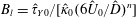
Table 1. Fracture flow categories: slow, normal and fast. First four rows define the category in terms of operational parameter ranges (see § 2.2). Remaining rows characterize the flow structure.

For each flow category we now use the rheological models outlined in § 2.1 together with (2.7) to estimate: (i) the width of the low-shear pseudo-plug; (ii) characteristic low-shear viscosities within the pseudo-plug; (iii) typical particle Stokes numbers within the pseudo-plug; (iv) minimal viscosities, found near the walls; (v) maximal local shear rates, found near the walls; and (vi) maximal particle Stokes numbers within the wall layers. These parameters are tabulated in the lower rows of table 1. This type of analysis is crude in not explicitly including particle migration effects, but does begin to paint a clearer picture of the flows encountered.
In general, the shear rate is relatively constant across the pseudo-plug and then increases continuously but sharply through the shear layers. Shear thinning together with the local strain-rate amplification of (2.3) result in significant centre-to-wall variations in local particle Stokes number (
 $St_{p}$
) given by
$St_{p}$
) given by
 $$\begin{eqnarray}St_{p}=\frac{\hat{\unicode[STIX]{x1D70C}}_{s}\hat{d}_{p}^{2}}{3\unicode[STIX]{x03C0}\hat{\unicode[STIX]{x1D702}}_{f}}\hat{\dot{\unicode[STIX]{x1D6FE}}}_{loc},\end{eqnarray}$$
which is interpreted as the ratio of the time scale for viscous drag to affect particle momentum and the characteristic time scale of the suspension:
 ${\sim}1/\hat{\dot{\unicode[STIX]{x1D6FE}}}_{loc}$
. Note that, since
${\sim}1/\hat{\dot{\unicode[STIX]{x1D6FE}}}_{loc}$
. Note that, since
 $\unicode[STIX]{x1D6FF}_{p}\ll 1$
, transverse variations in both effective viscosity and shear rate (due to the bulk imposed flow) are felt and evaluated locally on the particle length scale.
$\unicode[STIX]{x1D6FF}_{p}\ll 1$
, transverse variations in both effective viscosity and shear rate (due to the bulk imposed flow) are felt and evaluated locally on the particle length scale.
The Stokes number gives a measure of fluid–solid coupling. As expected, considering the full range of likely process and geometric conditions, the pseudo-plug regions are completely non-inertial in all flow types:
 $St_{p}\ll 1$
. The main differences are reflected in the size of the central low-shear region
$St_{p}\ll 1$
. The main differences are reflected in the size of the central low-shear region
 $y_{Y}$
. In moving from the pseudo-plug towards the wall,
$y_{Y}$
. In moving from the pseudo-plug towards the wall,
 $St_{p}$
increases due to both the increase in
$St_{p}$
increases due to both the increase in
 $\hat{\dot{\unicode[STIX]{x1D6FE}}}_{loc}$
and the decrease in
$\hat{\dot{\unicode[STIX]{x1D6FE}}}_{loc}$
and the decrease in
 $\hat{\unicode[STIX]{x1D702}}_{f}$
. For slow fracture flows we find
$\hat{\unicode[STIX]{x1D702}}_{f}$
. For slow fracture flows we find
 $St_{p}\lesssim 1$
throughout the fracture, whereas for normal flows
$St_{p}\lesssim 1$
throughout the fracture, whereas for normal flows
 $St_{p}\geqslant 1$
for approximately half of the sheared layer, approaching
$St_{p}\geqslant 1$
for approximately half of the sheared layer, approaching
 ${\sim}10$
at the walls. For fast flows we would have
${\sim}10$
at the walls. For fast flows we would have
 $1\lesssim St_{p}\lesssim 20$
over approximately half the fracture width, for typical 20/40 proppant.
$1\lesssim St_{p}\lesssim 20$
over approximately half the fracture width, for typical 20/40 proppant.
A representative particle Reynolds number is
 $$\begin{eqnarray}Re_{p}=\frac{\hat{\unicode[STIX]{x1D70C}}_{f}\hat{\dot{\unicode[STIX]{x1D6FE}}}_{loc}\hat{d}_{p}^{2}}{\hat{\unicode[STIX]{x1D702}}_{f}}=\frac{3\unicode[STIX]{x03C0}}{s}St_{p},\end{eqnarray}$$
which closely follows the variations in
 $St_{p}$
across the fracture as
$St_{p}$
across the fracture as
 $3\unicode[STIX]{x03C0}/s\sim O(1)$
. While
$3\unicode[STIX]{x03C0}/s\sim O(1)$
. While
 $St_{p}$
and
$St_{p}$
and
 $Re_{p}$
have similar size, the physical interpretation of these quantities is different. Larger
$Re_{p}$
have similar size, the physical interpretation of these quantities is different. Larger
 $Re_{p}\geqslant 1$
values imply that we enter a nonlinear regime of drag (viscous to inertial), whereas
$Re_{p}\geqslant 1$
values imply that we enter a nonlinear regime of drag (viscous to inertial), whereas
 $St_{p}\geqslant 1$
indicates that the particle velocity is not fully relaxed. The latter implies that the fluctuating components of the particle velocity becomes important. Commonly, this is represented via the granular or particle temperature
$St_{p}\geqslant 1$
indicates that the particle velocity is not fully relaxed. The latter implies that the fluctuating components of the particle velocity becomes important. Commonly, this is represented via the granular or particle temperature
 $\hat{\unicode[STIX]{x1D6E9}}\geqslant 0$
, which is the root-mean-square fluctuating velocity of the particle phase. Temperature
$\hat{\unicode[STIX]{x1D6E9}}\geqslant 0$
, which is the root-mean-square fluctuating velocity of the particle phase. Temperature
 $\hat{\unicode[STIX]{x1D6E9}}$
is present throughout the flow, but in Stokesian regimes (such as within the pseudo-plug)
$\hat{\unicode[STIX]{x1D6E9}}$
is present throughout the flow, but in Stokesian regimes (such as within the pseudo-plug)
 $\hat{\unicode[STIX]{x1D6E9}}$
becomes very small, serving primarily to regularize diffusive fluxes (see e.g. Nott & Brady Reference Nott and Brady1994). Particle temperature is more commonly used in kinetic theories of particle dynamics and in granular flows.
$\hat{\unicode[STIX]{x1D6E9}}$
becomes very small, serving primarily to regularize diffusive fluxes (see e.g. Nott & Brady Reference Nott and Brady1994). Particle temperature is more commonly used in kinetic theories of particle dynamics and in granular flows.
2.4 Modelling flow in the fracture
The main modelling challenge is to allow for a broad range of both bulk-scale flow effects (arising from geometry and process variations) and particle-scale effects as we traverse the fracture width. We adopt a continuum approach in which variables are interpreted as being volume-averaged over a suitably chosen local averaging volume, but not time-averaged. (Note that for typical
 $\unicode[STIX]{x1D6FF}_{p}\approx (2{-}4)\times 10^{-2}$
, we have 25–50 particle diameters across the fracture, so that we are close to the limit of validity of a continuum approach.) Operational choices, cyclical pumping (e.g. CFT), particle migration, the possibility of screen-out, etc. all combine to imply that models for transport along the fracture should consider a full range of
$\unicode[STIX]{x1D6FF}_{p}\approx (2{-}4)\times 10^{-2}$
, we have 25–50 particle diameters across the fracture, so that we are close to the limit of validity of a continuum approach.) Operational choices, cyclical pumping (e.g. CFT), particle migration, the possibility of screen-out, etc. all combine to imply that models for transport along the fracture should consider a full range of
 $\unicode[STIX]{x1D719}$
, from relatively dilute to concentrated suspensions.
$\unicode[STIX]{x1D719}$
, from relatively dilute to concentrated suspensions.
The description emerging is of a Stokesian pseudo-plug layer bounded by shear layers in which inertial and unsteady fluid–particle coupling effects are progressively important towards the walls. Variables specific to solid or liquid phases are phase-averaged, defined using the characteristic function of the phase, the local instantaneous variable (e.g. solids-phase velocity) and a suitable smoothing or weighting function
 ${\mathcal{G}}$
(see e.g. Drew Reference Drew1983, [). Our dimensional variables will be denoted with a
${\mathcal{G}}$
(see e.g. Drew Reference Drew1983, [). Our dimensional variables will be denoted with a
 $\hat{\cdot }$
throughout. The suspension mass and momentum balances are
$\hat{\cdot }$
throughout. The suspension mass and momentum balances are
 $$\begin{eqnarray}\displaystyle & \displaystyle \hat{\unicode[STIX]{x1D735}}\boldsymbol{\cdot }\hat{\boldsymbol{u}}=0, & \displaystyle\end{eqnarray}$$
 $$\begin{eqnarray}\displaystyle & \displaystyle \frac{\text{D}}{\text{D}\hat{t}}[\hat{\unicode[STIX]{x1D70C}}\hat{\boldsymbol{u}}]=\hat{\boldsymbol{b}}+\hat{\unicode[STIX]{x1D735}}\boldsymbol{\cdot }\hat{\unicode[STIX]{x1D72E}}, & \displaystyle\end{eqnarray}$$
where
 $\hat{\boldsymbol{u}}$
is the volume-averaged suspension velocity,
$\hat{\boldsymbol{u}}$
is the volume-averaged suspension velocity,
 $\hat{\boldsymbol{b}}$
and
$\hat{\boldsymbol{b}}$
and
 $\hat{\unicode[STIX]{x1D72E}}$
are the volume-averaged suspension body force and stress tensor, respectively (see Batchelor Reference Batchelor1970). The suspension stress
$\hat{\unicode[STIX]{x1D72E}}$
are the volume-averaged suspension body force and stress tensor, respectively (see Batchelor Reference Batchelor1970). The suspension stress
 $\hat{\unicode[STIX]{x1D72E}}$
is often decomposed into individual contributions from both fluid and solid phases:
$\hat{\unicode[STIX]{x1D72E}}$
is often decomposed into individual contributions from both fluid and solid phases:
 $$\begin{eqnarray}\hat{\unicode[STIX]{x1D72E}}=-\hat{p}_{f}\boldsymbol{I}+\hat{\unicode[STIX]{x1D749}}_{f}+\hat{\unicode[STIX]{x1D72E}}_{p}.\end{eqnarray}$$
The material derivative in (2.11) is
 $$\begin{eqnarray}\frac{\text{D}}{\text{D}\hat{t}}=\frac{\unicode[STIX]{x2202}}{\unicode[STIX]{x2202}\hat{t}}+\hat{\boldsymbol{u}}\boldsymbol{\cdot }\hat{\unicode[STIX]{x1D735}}.\end{eqnarray}$$
These equations are obtained by phase-averaging the individual equations for solid and liquid phases, then summing to eliminate the inter-phase terms. Thus, we also need to consider conservation equations for one phase, taken here as the solids phase:
 $$\begin{eqnarray}\displaystyle & \displaystyle \frac{\unicode[STIX]{x2202}\unicode[STIX]{x1D719}}{\unicode[STIX]{x2202}\hat{t}}+\hat{\unicode[STIX]{x1D735}}\boldsymbol{\cdot }[\unicode[STIX]{x1D719}\hat{\boldsymbol{u}}_{p}]=0, & \displaystyle\end{eqnarray}$$
 $$\begin{eqnarray}\displaystyle & \displaystyle \hat{\unicode[STIX]{x1D70C}}_{s}\frac{\text{D}_{p}}{\text{D}\hat{t}}\unicode[STIX]{x1D719}\hat{\boldsymbol{u}}_{p}=\hat{\unicode[STIX]{x1D735}}\boldsymbol{\cdot }\hat{\unicode[STIX]{x1D72E}}_{p}+\mathop{\sum }_{i=1}^{i=n_{p}}\int _{S_{i}}\boldsymbol{n}\boldsymbol{\cdot }\hat{\unicode[STIX]{x1D748}}{\mathcal{G}}\,\text{d}S+\hat{\boldsymbol{b}}. & \displaystyle\end{eqnarray}$$
Here
 $\hat{\boldsymbol{u}}_{p}$
is the phase-averaged particle velocity and
$\hat{\boldsymbol{u}}_{p}$
is the phase-averaged particle velocity and
 $\unicode[STIX]{x1D719}$
is the solids volume fraction. On the left-hand side of (2.15),
$\unicode[STIX]{x1D719}$
is the solids volume fraction. On the left-hand side of (2.15),
 $\text{D}_{p}/\text{D}\hat{t}$
denotes the material derivative using
$\text{D}_{p}/\text{D}\hat{t}$
denotes the material derivative using
 $\hat{\boldsymbol{u}}_{p}$
for the advective term. The first term on the right-hand side is the particle stress, i.e. particle contribution to the suspension stress. The second term is the volume-averaged traction on the particle surfaces and the last term is the average body force.
$\hat{\boldsymbol{u}}_{p}$
for the advective term. The first term on the right-hand side is the particle stress, i.e. particle contribution to the suspension stress. The second term is the volume-averaged traction on the particle surfaces and the last term is the average body force.
2.5 Developing the suspension balance framework
Diffusive and dispersive effects combine with the averaged forces acting on the solids phase to distribute the particles. The solid-phase mass conservation equation (2.14) is typically manipulated to give a transport equation for evolution of
 $\unicode[STIX]{x1D719}$
. Note that the phase averaging adopted preserves the instantaneous dynamics of each configuration, so that (2.14) has no diffusive flux. At least two general approaches have been taken to model particle-phase diffusion: (i) the diffusive flux approach of Leighton & Acrivos (Reference Leighton and Acrivos1987), modified by Phillips et al. (Reference Phillips, Armstrong, Brown, Graham and Abbott1992); and (ii) the SBM of Nott & Brady (Reference Nott and Brady1994).
$\unicode[STIX]{x1D719}$
. Note that the phase averaging adopted preserves the instantaneous dynamics of each configuration, so that (2.14) has no diffusive flux. At least two general approaches have been taken to model particle-phase diffusion: (i) the diffusive flux approach of Leighton & Acrivos (Reference Leighton and Acrivos1987), modified by Phillips et al. (Reference Phillips, Armstrong, Brown, Graham and Abbott1992); and (ii) the SBM of Nott & Brady (Reference Nott and Brady1994).
Following the SBM approach here, the relative velocity (
 $\hat{\boldsymbol{u}}_{r}=\hat{\boldsymbol{u}}_{s}-\hat{\boldsymbol{u}}_{f}$
) is substituted into (2.14) to give
$\hat{\boldsymbol{u}}_{r}=\hat{\boldsymbol{u}}_{s}-\hat{\boldsymbol{u}}_{f}$
) is substituted into (2.14) to give
 $$\begin{eqnarray}\displaystyle \frac{\unicode[STIX]{x2202}\unicode[STIX]{x1D719}}{\unicode[STIX]{x2202}\hat{t}}+\hat{\unicode[STIX]{x1D735}}\boldsymbol{\cdot }[\unicode[STIX]{x1D719}\hat{\boldsymbol{u}}] & = & \displaystyle -\hat{\unicode[STIX]{x1D735}}\boldsymbol{\cdot }[\unicode[STIX]{x1D719}(\hat{\boldsymbol{u}}_{p}-\hat{\boldsymbol{u}})]=-\hat{\unicode[STIX]{x1D735}}\boldsymbol{\cdot }[\unicode[STIX]{x1D719}(1-\unicode[STIX]{x1D719})\hat{\boldsymbol{u}}_{r}]\nonumber\\ \displaystyle & = & \displaystyle \hat{\unicode[STIX]{x1D735}}\boldsymbol{\cdot }[\unicode[STIX]{x1D719}(1-\unicode[STIX]{x1D719})\hat{M}(\hat{\unicode[STIX]{x1D702}}_{f},\hat{d}_{p},\unicode[STIX]{x1D719})\hat{\boldsymbol{f}}_{D}],\end{eqnarray}$$
where
 $\hat{M}$
denotes the particle mobility and
$\hat{M}$
denotes the particle mobility and
 $\hat{\boldsymbol{f}}_{D}$
is the phase-averaged particle drag force. The usual approach now is to consider (2.15) in the limit of small inertia, whereby
$\hat{\boldsymbol{f}}_{D}$
is the phase-averaged particle drag force. The usual approach now is to consider (2.15) in the limit of small inertia, whereby
 $\hat{\boldsymbol{f}}_{D}$
may be substituted into (2.16), leading to the divergence of the remaining terms on the right-hand side of (2.15).
$\hat{\boldsymbol{f}}_{D}$
may be substituted into (2.16), leading to the divergence of the remaining terms on the right-hand side of (2.15).
More recently Lhuillier (Reference Lhuillier2009) and Nott et al. (Reference Nott, Guazzelli and Pouliquen2011) have shown that the volume-averaged traction (second term on the right-hand side of (2.15)) may be expressed as the sum of a particle-averaged force and the negative divergence of the particle stress. In this sense, the particle stress does not contribute to the particle momentum equation. The only terms remaining on the right-hand side of (2.15) are the external body force and the particle-averaged force, which consists of the hydrodynamic forces, contact traction forces and interparticle forces. This questions the foundation of the SBM model in attributing the shear-induced particle migration to the divergence of particle-phase stress. However, Nott et al. (Reference Nott, Guazzelli and Pouliquen2011) showed that the particle-averaged force can itself be expressed in terms of an interphase drag force and the divergence of a stress tensor, which includes the effects of hydrodynamic, contact and interparticle forces. Consequently, the form of particle-phase momentum equation used in the SBM approach is correct, but using conventional closures for the interphase drag force and the stress tensor is currently under debate (see Lhuillier Reference Lhuillier2009; Nott et al. Reference Nott, Guazzelli and Pouliquen2011; Brady Reference Brady2015). Thus, we continue below to follow the classical SBM approach in developing our model, but incorporate the local viscosity of the shear-thinning yield stress suspension as outlined in § 2.1, and other necessary extensions.
One advantage of the SBM approach is that the particle temperature is included, which is helpful for modelling non-Stokesian particle effects present in fracture flows, as we do below, and in interpreting the results. We therefore replace (2.15) with the solid momentum equation:
 $$\begin{eqnarray}\hat{\unicode[STIX]{x1D70C}}_{s}\unicode[STIX]{x1D719}\frac{\text{D}_{p}}{\text{D}\hat{t}}\hat{\boldsymbol{u}}_{p}=\hat{\boldsymbol{f}}_{B}+\hat{\boldsymbol{f}}_{P}+\hat{\unicode[STIX]{x1D735}}\boldsymbol{\cdot }\hat{\unicode[STIX]{x1D72E}}_{p}.\end{eqnarray}$$
The phase-averaged forces acting on the particles contribute to two terms:
 $\hat{\boldsymbol{f}}_{B}$
representing the net solids-phase body force and
$\hat{\boldsymbol{f}}_{B}$
representing the net solids-phase body force and
 $\hat{\boldsymbol{f}}_{P}$
representing the hydrodynamic forces. The phase-averaged net solids-phase body force is
$\hat{\boldsymbol{f}}_{P}$
representing the hydrodynamic forces. The phase-averaged net solids-phase body force is
 $$\begin{eqnarray}\hat{\boldsymbol{f}}_{B}=\unicode[STIX]{x1D719}[\hat{\unicode[STIX]{x1D70C}}_{s}-\hat{\unicode[STIX]{x1D70C}}_{f}]\boldsymbol{g}.\end{eqnarray}$$
In this paper we simplify by assuming that the phase-averaged net particle force is given primarily by the drag force,
 $\hat{\boldsymbol{f}}_{P}\approx \hat{\boldsymbol{f}}_{D}$
, neglecting all other hydrodynamic particle forces. This in turn is modelled via a hindered settling closure:
$\hat{\boldsymbol{f}}_{P}\approx \hat{\boldsymbol{f}}_{D}$
, neglecting all other hydrodynamic particle forces. This in turn is modelled via a hindered settling closure:
 $$\begin{eqnarray}\hat{\boldsymbol{f}}_{D}=-\frac{3\unicode[STIX]{x1D719}\hat{\unicode[STIX]{x1D70C}}_{f}C_{D}(Re_{p,l})}{4h(\unicode[STIX]{x1D719})\hat{d}_{p}}|\hat{\boldsymbol{u}}_{r}|\hat{\boldsymbol{u}}_{r}.\end{eqnarray}$$
We adopt the same framework as Ovarlez and co-workers. In Ovarlez et al. (Reference Ovarlez, Bertrand, Coussot and Chateau2012) the authors study particle settling in yield stress fluids, perpendicular to the main direction of shear. They advocate using a Newtonian hindering function
 $h(\unicode[STIX]{x1D719})$
,
$h(\unicode[STIX]{x1D719})$
,
 $$\begin{eqnarray}h(\unicode[STIX]{x1D719})=\frac{1-\unicode[STIX]{x1D719}}{\unicode[STIX]{x1D702}_{r}(\unicode[STIX]{x1D719})},\end{eqnarray}$$
to modify the single-particle settling speed. They identify two limits (a plastic regime and a viscous regime) in each of which they use a drag law incorporating
 $\hat{\unicode[STIX]{x1D702}}_{f}(\hat{\dot{\unicode[STIX]{x1D6FE}}},\unicode[STIX]{x1D719})$
, as defined in (2.4). A quite similar usage of
$\hat{\unicode[STIX]{x1D702}}_{f}(\hat{\dot{\unicode[STIX]{x1D6FE}}},\unicode[STIX]{x1D719})$
, as defined in (2.4). A quite similar usage of
 $\hat{\unicode[STIX]{x1D702}}_{f}$
for fitting a drag coefficient is described in Tabuteau, Coussot & de Bruyn (Reference Tabuteau, Coussot and de Bruyn2007). The drag coefficient
$\hat{\unicode[STIX]{x1D702}}_{f}$
for fitting a drag coefficient is described in Tabuteau, Coussot & de Bruyn (Reference Tabuteau, Coussot and de Bruyn2007). The drag coefficient
 $C_{D}(Re_{p,l})$
is extended to cover inertial regimes, for which there are a number of similar closure laws. There is an advantage to having a drag coefficient closure law that is easily invertible, and consequently we adopt
$C_{D}(Re_{p,l})$
is extended to cover inertial regimes, for which there are a number of similar closure laws. There is an advantage to having a drag coefficient closure law that is easily invertible, and consequently we adopt
 $$\begin{eqnarray}C_{D}(Re_{p,l})=\left\{\begin{array}{@{}ll@{}}\displaystyle \frac{24}{Re_{p,l}},\quad & Re_{p,l}<1.4,\\[6.0pt] \displaystyle \frac{A_{CD}}{Re_{p,l}^{0.625}},\quad & 1.4\leqslant Re_{p,l}\leqslant 500,\end{array}\right.\end{eqnarray}$$
where
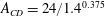 $A_{CD}=24/1.4^{0.375}$
. Note that the range of
$A_{CD}=24/1.4^{0.375}$
. Note that the range of
 $Re_{p,l}>500$
is unlikely to be attained. The Reynolds number is based on
$Re_{p,l}>500$
is unlikely to be attained. The Reynolds number is based on
 $\hat{\unicode[STIX]{x1D702}}_{f}(\hat{\dot{\unicode[STIX]{x1D6FE}}},\unicode[STIX]{x1D719})$
and
$\hat{\unicode[STIX]{x1D702}}_{f}(\hat{\dot{\unicode[STIX]{x1D6FE}}},\unicode[STIX]{x1D719})$
and
 $|\hat{\boldsymbol{u}}_{r}|$
, i.e.
$|\hat{\boldsymbol{u}}_{r}|$
, i.e.
 $$\begin{eqnarray}Re_{p,l}=\frac{\hat{\unicode[STIX]{x1D70C}}_{f}|\hat{\boldsymbol{u}}_{r}|\hat{d}_{p}}{\hat{\unicode[STIX]{x1D702}}_{f}}.\end{eqnarray}$$
Inverting (2.19), with the drag coefficient (2.21), leads straightforwardly to the relation
 $\hat{\boldsymbol{u}}_{r}=-\hat{M}(\unicode[STIX]{x1D719},\hat{\dot{\unicode[STIX]{x1D6FE}}},|\hat{\boldsymbol{f}}_{D}|)\hat{\boldsymbol{f}}_{D}$
, required for (2.16). We specify a dimensionless version of the mobility
$\hat{\boldsymbol{u}}_{r}=-\hat{M}(\unicode[STIX]{x1D719},\hat{\dot{\unicode[STIX]{x1D6FE}}},|\hat{\boldsymbol{f}}_{D}|)\hat{\boldsymbol{f}}_{D}$
, required for (2.16). We specify a dimensionless version of the mobility
 $\hat{M}$
later.
$\hat{M}$
later.
Returning to the SBM derivation, it is assumed that the left-hand side of (2.17) is relatively small (which would hold, for example, in conditions where the flow is steady, rectilinear and fully developed). In this case, we may write
 $$\begin{eqnarray}\hat{\boldsymbol{f}}_{D}\approx -[\hat{\boldsymbol{f}}_{B}+\hat{\unicode[STIX]{x1D735}}\boldsymbol{\cdot }\hat{\unicode[STIX]{x1D72E}}_{p}],\end{eqnarray}$$
and the solids mass conservation equation becomes
 $$\begin{eqnarray}\frac{\unicode[STIX]{x2202}\unicode[STIX]{x1D719}}{\unicode[STIX]{x2202}\hat{t}}+\hat{\unicode[STIX]{x1D735}}\boldsymbol{\cdot }[\unicode[STIX]{x1D719}\hat{\boldsymbol{u}}]=-\hat{\unicode[STIX]{x1D735}}\boldsymbol{\cdot }[\unicode[STIX]{x1D719}(1-\unicode[STIX]{x1D719})\hat{M}(\unicode[STIX]{x1D719},\hat{\dot{\unicode[STIX]{x1D6FE}}},|\hat{\boldsymbol{f}}_{D}|)(\hat{\boldsymbol{f}}_{B}+\hat{\unicode[STIX]{x1D735}}\boldsymbol{\cdot }\hat{\unicode[STIX]{x1D72E}}_{p})].\end{eqnarray}$$
The particle stress tensor is usually modelled by the expression
 $$\begin{eqnarray}\hat{\unicode[STIX]{x1D72E}}_{p}=-\hat{\unicode[STIX]{x1D6F1}}\unicode[STIX]{x1D655}+\hat{\unicode[STIX]{x1D702}}_{f}\unicode[STIX]{x1D702}_{p}(\unicode[STIX]{x1D719})\hat{\dot{\unicode[STIX]{x1D738}}}\end{eqnarray}$$
(see e.g. Fang et al.
Reference Fang, Mammoli, Brady, Ingber, Mondy and Graham2002). The second term in (2.25) is the particle shear stress term. The bulk rate-of-strain tensor for the suspension is
 $\hat{\dot{\unicode[STIX]{x1D738}}}=\hat{\dot{\unicode[STIX]{x1D6FE}}}_{ij}$
. Note that the bulk suspension strain rate is
$\hat{\dot{\unicode[STIX]{x1D738}}}=\hat{\dot{\unicode[STIX]{x1D6FE}}}_{ij}$
. Note that the bulk suspension strain rate is
 $$\begin{eqnarray}\hat{\dot{\unicode[STIX]{x1D6FE}}}=\left[\frac{1}{2}\mathop{\sum }_{i,j=1}^{3}\hat{\dot{\unicode[STIX]{x1D6FE}}}_{ij}^{2}\right]^{1/2}.\end{eqnarray}$$
The first term in (2.25) is a product of the particle pressure
 $\hat{\unicode[STIX]{x1D6F1}}$
and the tensor
$\hat{\unicode[STIX]{x1D6F1}}$
and the tensor
 $\unicode[STIX]{x1D655}$
, through which we account for normal stress differences. It is argued that a reasonable approximation to the tensor
$\unicode[STIX]{x1D655}$
, through which we account for normal stress differences. It is argued that a reasonable approximation to the tensor
 $\unicode[STIX]{x1D655}$
is
$\unicode[STIX]{x1D655}$
is
 $$\begin{eqnarray}\unicode[STIX]{x1D655}=\left(\begin{array}{@{}ccc@{}}\unicode[STIX]{x1D706}_{1} & 0 & 0\\ 0 & \unicode[STIX]{x1D706}_{2} & 0\\ 0 & 0 & \unicode[STIX]{x1D706}_{3}\end{array}\right),\end{eqnarray}$$
where the directions
 $x_{1}$
and
$x_{1}$
and
 $x_{2}$
are in the plane of shear (here this would be locally aligned with the mean flow along the fracture). According to the scaling,
$x_{2}$
are in the plane of shear (here this would be locally aligned with the mean flow along the fracture). According to the scaling,
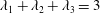 $\unicode[STIX]{x1D706}_{1}+\unicode[STIX]{x1D706}_{2}+\unicode[STIX]{x1D706}_{3}=3$
, and from Brady & Morris (Reference Brady and Morris1997), a common choice for shear flow is
$\unicode[STIX]{x1D706}_{1}+\unicode[STIX]{x1D706}_{2}+\unicode[STIX]{x1D706}_{3}=3$
, and from Brady & Morris (Reference Brady and Morris1997), a common choice for shear flow is
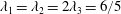 $\unicode[STIX]{x1D706}_{1}=\unicode[STIX]{x1D706}_{2}=2\unicode[STIX]{x1D706}_{3}=6/5$
. Other choices can be made if there is specific knowledge of the normal stress differences. The particle pressure is modelled using the particle temperature in place of the strain rate, considering that
$\unicode[STIX]{x1D706}_{1}=\unicode[STIX]{x1D706}_{2}=2\unicode[STIX]{x1D706}_{3}=6/5$
. Other choices can be made if there is specific knowledge of the normal stress differences. The particle pressure is modelled using the particle temperature in place of the strain rate, considering that
 $\hat{\dot{\unicode[STIX]{x1D6FE}}}^{2}\propto \hat{d}_{p}^{-2}\hat{\unicode[STIX]{x1D6E9}}$
in a homogeneous suspension. The form selected is
$\hat{\dot{\unicode[STIX]{x1D6FE}}}^{2}\propto \hat{d}_{p}^{-2}\hat{\unicode[STIX]{x1D6E9}}$
in a homogeneous suspension. The form selected is
 $$\begin{eqnarray}\hat{\unicode[STIX]{x1D6F1}}=\hat{\unicode[STIX]{x1D702}}_{f}\hat{d}_{p}^{-1}\hat{\unicode[STIX]{x1D6E9}}^{1/2}p(\unicode[STIX]{x1D719}),\quad p(\unicode[STIX]{x1D719})=2\sqrt{3}k_{\unicode[STIX]{x1D719}}\unicode[STIX]{x1D719}^{1/2}(\unicode[STIX]{x1D702}_{p})^{{\mathcal{A}}}.\end{eqnarray}$$
An evolution equation for
 $\hat{\unicode[STIX]{x1D6E9}}$
is derived in Nott & Brady (Reference Nott and Brady1994) as a simplified form of the mechanical energy balance for the particle phase:
$\hat{\unicode[STIX]{x1D6E9}}$
is derived in Nott & Brady (Reference Nott and Brady1994) as a simplified form of the mechanical energy balance for the particle phase:
 $$\begin{eqnarray}3\hat{\unicode[STIX]{x1D70C}}_{s}\unicode[STIX]{x1D719}C(\unicode[STIX]{x1D719})\frac{\text{D}_{p}\hat{\unicode[STIX]{x1D6E9}}}{\text{D}\hat{t}}=\hat{\unicode[STIX]{x1D72E}}_{p},\quad \hat{\dot{\unicode[STIX]{x1D738}}}+4\sqrt{3}\hat{\unicode[STIX]{x1D702}}_{f}\hat{d}_{p}^{-2}\unicode[STIX]{x1D6FD}(\unicode[STIX]{x1D719})\hat{\unicode[STIX]{x1D6E9}}^{1/2}|\hat{\boldsymbol{u}}_{r}|-12\hat{\unicode[STIX]{x1D702}}_{f}\hat{d}_{p}^{-2}\unicode[STIX]{x1D6FC}(\unicode[STIX]{x1D719})\hat{\unicode[STIX]{x1D6E9}}-\hat{\unicode[STIX]{x1D735}}\boldsymbol{\cdot }\hat{\boldsymbol{q}}.\end{eqnarray}$$
There are slight differences due to our preference to work with the particle diameter rather than radius, and a factor of
 $1/3$
absent in Nott & Brady (Reference Nott and Brady1994), compared to the usual definition of particle temperature. The heat-capacity term
$1/3$
absent in Nott & Brady (Reference Nott and Brady1994), compared to the usual definition of particle temperature. The heat-capacity term
 $C(\unicode[STIX]{x1D719})$
is not specified, and not used below. The functions
$C(\unicode[STIX]{x1D719})$
is not specified, and not used below. The functions
 $\unicode[STIX]{x1D6FC}(\unicode[STIX]{x1D719})$
and
$\unicode[STIX]{x1D6FC}(\unicode[STIX]{x1D719})$
and
 $\unicode[STIX]{x1D6FD}(\unicode[STIX]{x1D719})$
are specified semi-empirically by considering different limits of the model. The field
$\unicode[STIX]{x1D6FD}(\unicode[STIX]{x1D719})$
are specified semi-empirically by considering different limits of the model. The field
 $\hat{\boldsymbol{q}}$
represents the phase-averaged fluctuating component of the solids-phase dissipation, i.e.
$\hat{\boldsymbol{q}}$
represents the phase-averaged fluctuating component of the solids-phase dissipation, i.e.
 $$\begin{eqnarray}\hat{\boldsymbol{q}}=-\langle \hat{\unicode[STIX]{x1D72E}}_{p}^{\prime }\boldsymbol{\cdot }(\hat{\boldsymbol{u}}_{p}-\langle \hat{\boldsymbol{u}}\rangle _{p})\rangle ,\end{eqnarray}$$
which is modelled via a Fourier-type ‘conductive heat flux’ law,
 $$\begin{eqnarray}\hat{\boldsymbol{q}}=-3\hat{\unicode[STIX]{x1D702}}_{f}\unicode[STIX]{x1D705}_{\unicode[STIX]{x1D6E9}}(\unicode[STIX]{x1D719})\hat{\unicode[STIX]{x1D735}}\hat{\unicode[STIX]{x1D6E9}}.\end{eqnarray}$$
Although phenomenological in many respects the above model has proven successful in predicting solids-phase distributions in pressure-driven shear flows and many others.
2.6 Unsteady inertial effects
The model outlined above is the standard SBM approach, extended to include non-Newtonian frac fluids (§ 2.1) and steady inertial effects via the nonlinear drag regime. In fracturing flows, within the shear layers approaching the walls, unsteady inertial effects also arise. We now look in more detail at the response of the suspension in the different parts of the flow, with the aim of developing a rational framework that covers these effects.
Following Cassar, Nicolas & Pouliquen (Reference Cassar, Nicolas and Pouliquen2005) and Andreotti, Forterre & Pouliquen (Reference Andreotti, Forterre and Pouliquen2013) we consider a particle that accelerates within the suspension, under the action of a pressure
 $\hat{P}$
and drag force
$\hat{P}$
and drag force
 $\hat{F}_{d}$
. The particle responds on at least three different microscopic time scales related to rearrangement of the suspension. Either
$\hat{F}_{d}$
. The particle responds on at least three different microscopic time scales related to rearrangement of the suspension. Either
 $\hat{P}$
is balanced by pure acceleration (leading to
$\hat{P}$
is balanced by pure acceleration (leading to
 $\hat{t}_{1}\sim \hat{\unicode[STIX]{x1D70C}}_{s}\hat{\unicode[STIX]{x1D6E9}}^{1/2}\hat{d}_{p}/\hat{P}$
), or
$\hat{t}_{1}\sim \hat{\unicode[STIX]{x1D70C}}_{s}\hat{\unicode[STIX]{x1D6E9}}^{1/2}\hat{d}_{p}/\hat{P}$
), or
 $\hat{P}$
is balanced by
$\hat{P}$
is balanced by
 $\hat{F}_{d}$
. The latter leads to
$\hat{F}_{d}$
. The latter leads to
 $\hat{t}_{2}~({\sim}\hat{\unicode[STIX]{x1D702}}_{f}/\hat{P})$
if the drag is principally viscous, or to
$\hat{t}_{2}~({\sim}\hat{\unicode[STIX]{x1D702}}_{f}/\hat{P})$
if the drag is principally viscous, or to
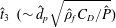 $\hat{t}_{3}~({\sim}\hat{d}_{p}\sqrt{\hat{\unicode[STIX]{x1D70C}}_{f}C_{D}/\hat{P}})$
if the drag is principally inertial. When the suspension is itself under shear, there is also a macroscopic time scale arising from the strain rate. We have seen that the bulk strain rate (
$\hat{t}_{3}~({\sim}\hat{d}_{p}\sqrt{\hat{\unicode[STIX]{x1D70C}}_{f}C_{D}/\hat{P}})$
if the drag is principally inertial. When the suspension is itself under shear, there is also a macroscopic time scale arising from the strain rate. We have seen that the bulk strain rate (
 $\hat{\dot{\unicode[STIX]{x1D6FE}}}$
) is felt locally as
$\hat{\dot{\unicode[STIX]{x1D6FE}}}$
) is felt locally as
 $\hat{\dot{\unicode[STIX]{x1D6FE}}}_{loc}$
, which is still macroscopic on the particle scale.
$\hat{\dot{\unicode[STIX]{x1D6FE}}}_{loc}$
, which is still macroscopic on the particle scale.
Comparison of the macroscopic time scale
 $(\hat{\dot{\unicode[STIX]{x1D6FE}}}_{loc}^{-1})$
, with each of
$(\hat{\dot{\unicode[STIX]{x1D6FE}}}_{loc}^{-1})$
, with each of
 $\hat{t}_{1}$
–
$\hat{t}_{1}$
–
 $\hat{t}_{3}$
leads to three dimensionless groups, the relative size of which determines the dominant characteristic behaviour of the suspension, i.e. at different positions across the fracture and in different types of bulk flow. For example, when
$\hat{t}_{3}$
leads to three dimensionless groups, the relative size of which determines the dominant characteristic behaviour of the suspension, i.e. at different positions across the fracture and in different types of bulk flow. For example, when
 $\hat{t}_{1}\gtrsim \hat{t}_{2}$
and
$\hat{t}_{1}\gtrsim \hat{t}_{2}$
and
 $\hat{t}_{1}\gtrsim \hat{t}_{3}$
, the rate-limiting microscopic time scale is
$\hat{t}_{1}\gtrsim \hat{t}_{3}$
, the rate-limiting microscopic time scale is
 $\hat{t}_{1}$
and suspension behaviour is described primarily by
$\hat{t}_{1}$
and suspension behaviour is described primarily by
 $I=\hat{\dot{\unicode[STIX]{x1D6FE}}}\hat{t}_{1}$
(case I). In this regime particle inertia dominates. If
$I=\hat{\dot{\unicode[STIX]{x1D6FE}}}\hat{t}_{1}$
(case I). In this regime particle inertia dominates. If
 $\hat{t}_{2}\gtrsim \hat{t}_{1}$
and
$\hat{t}_{2}\gtrsim \hat{t}_{1}$
and
 $\hat{t}_{2}\gtrsim \hat{t}_{3}$
, then
$\hat{t}_{2}\gtrsim \hat{t}_{3}$
, then
 $\hat{t}_{2}$
is the rate-limiting microscopic time scale and suspension behaviour is described primarily by
$\hat{t}_{2}$
is the rate-limiting microscopic time scale and suspension behaviour is described primarily by
 $J=\hat{\dot{\unicode[STIX]{x1D6FE}}}\hat{t}_{2}$
(case II: viscous drag regime). Finally, when
$J=\hat{\dot{\unicode[STIX]{x1D6FE}}}\hat{t}_{2}$
(case II: viscous drag regime). Finally, when
 $\hat{t}_{3}$
is rate-limiting, we expect
$\hat{t}_{3}$
is rate-limiting, we expect
 $J_{I}=\hat{\dot{\unicode[STIX]{x1D6FE}}}\hat{t}_{3}$
to describe the suspension behaviour (case III: inertial drag regime).
$J_{I}=\hat{\dot{\unicode[STIX]{x1D6FE}}}\hat{t}_{3}$
to describe the suspension behaviour (case III: inertial drag regime).
These three microscopic regimes are plotted schematically in figure 2. Note that the drag coefficient
 $C_{D}$
is used on the vertical axis in order to capture both viscous and inertial balances. The fluctuating component of velocity has characteristic size
$C_{D}$
is used on the vertical axis in order to capture both viscous and inertial balances. The fluctuating component of velocity has characteristic size
 $\hat{\unicode[STIX]{x1D6E9}}^{1/2}$
, which is used to define a (fluctuating) particle Reynolds number:
$\hat{\unicode[STIX]{x1D6E9}}^{1/2}$
, which is used to define a (fluctuating) particle Reynolds number:
 $$\begin{eqnarray}Re_{p,\unicode[STIX]{x1D6E9}}=\frac{\hat{\unicode[STIX]{x1D70C}}_{f}\hat{d}_{p}\hat{\unicode[STIX]{x1D6E9}}^{1/2}}{\hat{\unicode[STIX]{x1D702}}_{f}}.\end{eqnarray}$$
Using
 $Re_{p,\unicode[STIX]{x1D6E9}}$
in the usual Stokesian drag law allows us to evaluate
$Re_{p,\unicode[STIX]{x1D6E9}}$
in the usual Stokesian drag law allows us to evaluate
 $\hat{t}_{1}/\hat{t}_{2}=\sqrt{sRe_{p,\unicode[STIX]{x1D6E9}}/24}\propto \sqrt{St_{p,\unicode[STIX]{x1D6E9}}}$
. One can similarly evaluate
$\hat{t}_{1}/\hat{t}_{2}=\sqrt{sRe_{p,\unicode[STIX]{x1D6E9}}/24}\propto \sqrt{St_{p,\unicode[STIX]{x1D6E9}}}$
. One can similarly evaluate
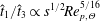 $\hat{t}_{1}/\hat{t}_{3}\propto s^{1/2}Re_{p,\unicode[STIX]{x1D6E9}}^{5/16}$
, over the inertial range likely in this process (and eventually
$\hat{t}_{1}/\hat{t}_{3}\propto s^{1/2}Re_{p,\unicode[STIX]{x1D6E9}}^{5/16}$
, over the inertial range likely in this process (and eventually
 $\hat{t}_{1}/\hat{t}_{3}\propto s^{1/2}$
as
$\hat{t}_{1}/\hat{t}_{3}\propto s^{1/2}$
as
 $Re_{p,\unicode[STIX]{x1D6E9}}\rightarrow \infty$
).
$Re_{p,\unicode[STIX]{x1D6E9}}\rightarrow \infty$
).
In each microscopic regime it is possible to derive order-of-magnitude estimates for the key terms in the solids-phase conservation laws, as was done by Jenkins & McTigue (Reference Jenkins, McTigue, Joseph and Schaeffer1990) for the granular regime; see table 2. In table 2,
 ${\hat{h}}=\hat{d}_{p}[\unicode[STIX]{x1D702}_{r}(\unicode[STIX]{x1D719})/(1-\unicode[STIX]{x1D719})]^{-1/2}$
denotes a representative particle separation, estimated consistently with our earlier treatment of the local strain rate. Particle conductivity and dissipation terms are described later with the transport equation for
${\hat{h}}=\hat{d}_{p}[\unicode[STIX]{x1D702}_{r}(\unicode[STIX]{x1D719})/(1-\unicode[STIX]{x1D719})]^{-1/2}$
denotes a representative particle separation, estimated consistently with our earlier treatment of the local strain rate. Particle conductivity and dissipation terms are described later with the transport equation for
 $\hat{\unicode[STIX]{x1D6E9}}$
(see appendix A).
$\hat{\unicode[STIX]{x1D6E9}}$
(see appendix A).

Figure 2. Variation of the local suspension regimes with slow, normal and fast fracture flows. The arrows indicate the variation across the fracture from the pseudo-plug in the centre to more inertial regimes at the fracture walls (styled after figure 7.13 in Andreotti et al. (Reference Andreotti, Forterre and Pouliquen2013)).
Table 2. Scalings of solid-phase properties for cases I, II and II.

It remains to interpret the different fracture flows in terms of the localized suspension characteristics described above. To do this we balance
 $\hat{\dot{\unicode[STIX]{x1D6FE}}}_{loc}\sim \hat{\unicode[STIX]{x1D6E9}}^{1/2}/d_{p}$
, to enable us to relate
$\hat{\dot{\unicode[STIX]{x1D6FE}}}_{loc}\sim \hat{\unicode[STIX]{x1D6E9}}^{1/2}/d_{p}$
, to enable us to relate
 $St_{p,\unicode[STIX]{x1D6E9}}$
to
$St_{p,\unicode[STIX]{x1D6E9}}$
to
 $St_{p}$
. Note that
$St_{p}$
. Note that
 $\hat{\dot{\unicode[STIX]{x1D6FE}}}_{loc}$
is imposed by the macroscopic flow, whereas
$\hat{\dot{\unicode[STIX]{x1D6FE}}}_{loc}$
is imposed by the macroscopic flow, whereas
 $\hat{\unicode[STIX]{x1D6E9}}^{1/2}/d_{p}$
is a measure of the local response of the fluctuating particle velocity to this strain rate. Figure 2 shows schematically where the (process-scale) fracture flows ‘live’ in terms of the
$\hat{\unicode[STIX]{x1D6E9}}^{1/2}/d_{p}$
is a measure of the local response of the fluctuating particle velocity to this strain rate. Figure 2 shows schematically where the (process-scale) fracture flows ‘live’ in terms of the
 $(I,J,J_{I})$
cartoon that indicates microscopic regimes. The arrows indicate the variation across the fracture from the pseudo-plug in the centre to more inertial and unsteady regimes at the fracture walls.
$(I,J,J_{I})$
cartoon that indicates microscopic regimes. The arrows indicate the variation across the fracture from the pseudo-plug in the centre to more inertial and unsteady regimes at the fracture walls.
This schematic indicates to us how non-Stokesian effects enter as we move across the fracture width, and table 2 suggests the appropriate scaling for extending the different terms in the SBM. Although we take this approach below, it is not the only way to model and include inertial/unsteady effects in the SBM. An alternative approach is to introduce an
 $O(Re_{p,\unicode[STIX]{x1D6E9}})$
‘correction’ into the energy equation of the SBM (and into the other closures), drawing from kinetic theory. Closure models in these regimes have been developed by Koch and co-workers (e.g. Sangani et al.
Reference Sangani, Mo, Tsao and Koch1996; Wylie, Koch & Ladd Reference Wylie, Koch and Ladd2003), targeted primarily at dense inertial gas suspensions, but also applicable to liquid suspensions with sufficiently large density ratio,
$O(Re_{p,\unicode[STIX]{x1D6E9}})$
‘correction’ into the energy equation of the SBM (and into the other closures), drawing from kinetic theory. Closure models in these regimes have been developed by Koch and co-workers (e.g. Sangani et al.
Reference Sangani, Mo, Tsao and Koch1996; Wylie, Koch & Ladd Reference Wylie, Koch and Ladd2003), targeted primarily at dense inertial gas suspensions, but also applicable to liquid suspensions with sufficiently large density ratio,
 $s$
. An application of this style of model to slurry flows in fractures is developed by Eskin & Miller (Reference Eskin and Miller2008). The gas kinetic theory closures are not strictly applicable for the
$s$
. An application of this style of model to slurry flows in fractures is developed by Eskin & Miller (Reference Eskin and Miller2008). The gas kinetic theory closures are not strictly applicable for the
 $s$
typical of fracturing flows, but this body of work does indicate the order of
$s$
typical of fracturing flows, but this body of work does indicate the order of
 $Re_{p,\unicode[STIX]{x1D6E9}}$
correction. We outline this approach and compare with the direct scaling approach in appendix B.
$Re_{p,\unicode[STIX]{x1D6E9}}$
correction. We outline this approach and compare with the direct scaling approach in appendix B.
In the Stokesian regime (case II) these scales are well known and those in table 2 are consistent with those of the SBM in Nott & Brady (Reference Nott and Brady1994). Comparing the scalings for case I with those for case II gives us the extension to the SBM closures as we transition from Stokesian to the granular regime. Comparing the scalings for case III with those for case II gives us the extension to the SBM closures as we transition from Stokesian to the inertial hydrodynamic regime. The results of making these comparisons are illustrated in table 3. We observe that (dimensionally) the first column has a prefactor
 $sRe_{p,\unicode[STIX]{x1D6E9}}$
compared to the Stokesian regime (case II), and the third column has a prefactor
$sRe_{p,\unicode[STIX]{x1D6E9}}$
compared to the Stokesian regime (case II), and the third column has a prefactor
 $Re_{p,\unicode[STIX]{x1D6E9}}$
. The case III scalings are based on a fully inertial regime (in which the drag coefficient becomes Reynolds-invariant), but in this application we are still in the weakly inertial regime at the particle scale. Typically
$Re_{p,\unicode[STIX]{x1D6E9}}$
. The case III scalings are based on a fully inertial regime (in which the drag coefficient becomes Reynolds-invariant), but in this application we are still in the weakly inertial regime at the particle scale. Typically
 $s\approx 2.65$
(sand–water), or sometimes
$s\approx 2.65$
(sand–water), or sometimes
 $s\approx 3{-}4$
(ceramic proppants), so that the relevant extensions to the Stokesian closures may be regarded as being of order
$s\approx 3{-}4$
(ceramic proppants), so that the relevant extensions to the Stokesian closures may be regarded as being of order
 $Re_{p,\unicode[STIX]{x1D6E9}}$
.
$Re_{p,\unicode[STIX]{x1D6E9}}$
.
Table 3. Forms of solid-phase properties for cases I, II and III, scaled with the Stokesian case.

Although we have used table 2 directly, the same order of magnitudes result on using the micro–macro time scale balances outlined above, which has some current popularity. A recent example of this is from Trulsson et al. (Reference Trulsson, Andreotti and Claudin2012), who use a 2D computational approach to model the transition between case I and case II regimes. They show that the
 $sRe_{p,\unicode[STIX]{x1D6E9}}$
prefactor is multiplied by a constant (
$sRe_{p,\unicode[STIX]{x1D6E9}}$
prefactor is multiplied by a constant (
 ${\approx}0.6$
for the ranges studied). This suggests that the scaling approach followed here is valid and that we may also expect
${\approx}0.6$
for the ranges studied). This suggests that the scaling approach followed here is valid and that we may also expect
 $O(1)$
constant multipliers to the prefactors listed in table 3. Determination of these multipliers, however, requires extensive further experimentation and/or simulation, which is not our intent here. Instead, we assume constant unit multipliers for simplicity, which leads to the following extensions to the SBM closures:
$O(1)$
constant multipliers to the prefactors listed in table 3. Determination of these multipliers, however, requires extensive further experimentation and/or simulation, which is not our intent here. Instead, we assume constant unit multipliers for simplicity, which leads to the following extensions to the SBM closures:
 $$\begin{eqnarray}\displaystyle & \displaystyle \unicode[STIX]{x1D702}_{s}=\unicode[STIX]{x1D702}_{p}(\unicode[STIX]{x1D719})(1+sRe_{p,\unicode[STIX]{x1D6E9}}), & \displaystyle\end{eqnarray}$$
 $$\begin{eqnarray}\displaystyle & \displaystyle \unicode[STIX]{x1D6F1}=\unicode[STIX]{x1D702}_{f}\unicode[STIX]{x1D6E9}^{1/2}2\sqrt{3}k_{\unicode[STIX]{x1D719}}\unicode[STIX]{x1D719}^{1/2}\unicode[STIX]{x1D702}_{p}(\unicode[STIX]{x1D719})(1+sRe_{p,\unicode[STIX]{x1D6E9}}), & \displaystyle\end{eqnarray}$$
 $$\begin{eqnarray}\displaystyle & \displaystyle \unicode[STIX]{x1D6FC}=\frac{k_{\unicode[STIX]{x1D6FC}}\unicode[STIX]{x1D702}_{p}(\unicode[STIX]{x1D719})}{\unicode[STIX]{x1D719}}(1+sRe_{p,\unicode[STIX]{x1D6E9}}), & \displaystyle\end{eqnarray}$$
 $$\begin{eqnarray}\displaystyle & \displaystyle \unicode[STIX]{x1D705}_{\unicode[STIX]{x1D6E9}}=k_{c}\unicode[STIX]{x1D702}_{p}(\unicode[STIX]{x1D719})(1+sRe_{p,\unicode[STIX]{x1D6E9}}). & \displaystyle\end{eqnarray}$$
3 Dimensionless model
To clarify the different physical effects present in the model derived in § 2.4, we scale the various equations. We assume a (locally) Cartesian coordinate system at any position along the fracture, with
 $\hat{x}$
in the direction of flow,
$\hat{x}$
in the direction of flow,
 ${\hat{y}}$
measured across the fracture and
${\hat{y}}$
measured across the fracture and
 $\hat{z}$
measured downwards, aligned with gravity. We define dimensionless coordinates and velocity components as
$\hat{z}$
measured downwards, aligned with gravity. We define dimensionless coordinates and velocity components as
 $$\begin{eqnarray}(x,y,z)=\left(\frac{\hat{x}}{\hat{L}_{t}},\frac{{\hat{y}}}{\hat{D}},\frac{\hat{z}}{\hat{L}_{t}}\right),\quad (u,v,w)=\left(\frac{\hat{u} }{\hat{U} _{0}},\unicode[STIX]{x1D6FF}_{t}\frac{\hat{v}}{\hat{U} _{0}},\frac{{\hat{w}}}{\hat{U} _{0}}\right),\end{eqnarray}$$
and time is scaled with
 $\hat{L}_{t}/\hat{U} _{0}$
. The scaled fracture has walls at
$\hat{L}_{t}/\hat{U} _{0}$
. The scaled fracture has walls at
 $y=-y_{w,-}(x,z)$
and
$y=-y_{w,-}(x,z)$
and
 $y=y_{w,+}(x,z)$
. Recall that
$y=y_{w,+}(x,z)$
. Recall that
 $\unicode[STIX]{x1D6FF}_{t}=\hat{D}/\hat{L}_{t}\ll 1$
reflects the local aspect ratio of the fracture (
$\unicode[STIX]{x1D6FF}_{t}=\hat{D}/\hat{L}_{t}\ll 1$
reflects the local aspect ratio of the fracture (
 $\unicode[STIX]{x1D6FF}_{t}^{-1}$
is thus a representative distance along the fracture over which significant geometric changes take place). Components of the particle velocity and relative velocity are scaled in identical fashion. On applying this scaling, it follows that the leading-order strain rates are shear components in the plane of the fracture, of size
$\unicode[STIX]{x1D6FF}_{t}^{-1}$
is thus a representative distance along the fracture over which significant geometric changes take place). Components of the particle velocity and relative velocity are scaled in identical fashion. On applying this scaling, it follows that the leading-order strain rates are shear components in the plane of the fracture, of size
 $\hat{U} _{0}/\hat{D}$
, with extensional strain rates
$\hat{U} _{0}/\hat{D}$
, with extensional strain rates
 $O(\unicode[STIX]{x1D6FF}_{t})$
smaller.
$O(\unicode[STIX]{x1D6FF}_{t})$
smaller.
The extensional strain rates are felt primarily where the shear components vanish. As discussed in § 2.2, the slowly varying geometry tends to induce a pseudo-plug region in the fracture midplane within which the yield stress is marginally exceeded and the strain rates are of the size of the extensional strain rate. Although there are analyses of velocity profiles within such regions, these are geometry-specific and amount only to an
 $O(\unicode[STIX]{x1D6FF}_{t})$
correction. To include this geometric effect in a general (but phenomenological) way, we simply modify the strain rate as
$O(\unicode[STIX]{x1D6FF}_{t})$
correction. To include this geometric effect in a general (but phenomenological) way, we simply modify the strain rate as
 $$\begin{eqnarray}\hat{\dot{\unicode[STIX]{x1D6FE}}}=\frac{\hat{U} _{0}}{\hat{D}}\dot{\unicode[STIX]{x1D6FE}}=\frac{\hat{U} _{0}}{\hat{D}}\left[\left(\frac{\unicode[STIX]{x2202}u}{\unicode[STIX]{x2202}y}\right)^{2}+\left(\frac{\unicode[STIX]{x2202}w}{\unicode[STIX]{x2202}y}\right)^{2}+\unicode[STIX]{x1D6FF}_{t}^{2}\right]^{1/2},\end{eqnarray}$$
wherever it appears in the effective viscosity. This is essentially a regularization: the strain rate will not vanish in the pseudo-plug and the effective viscosity will remain finite. In the sheared layers (since
 $\unicode[STIX]{x1D6FF}_{t}\ll 1$
), this results in a minor perturbation to the leading-order shear stresses and flow.
$\unicode[STIX]{x1D6FF}_{t}\ll 1$
), this results in a minor perturbation to the leading-order shear stresses and flow.
As the leading-order strain rates are
 ${\sim}\hat{U} _{0}/\hat{D}$
, we define a viscosity scale
${\sim}\hat{U} _{0}/\hat{D}$
, we define a viscosity scale
 $\hat{\unicode[STIX]{x1D702}}_{0}$
as
$\hat{\unicode[STIX]{x1D702}}_{0}$
as
 $$\begin{eqnarray}\hat{\unicode[STIX]{x1D702}}_{0}=\hat{\unicode[STIX]{x1D705}}_{0}\left(\frac{\hat{U} _{0}}{\hat{D}}\right)^{n-1},\end{eqnarray}$$
which we use to scale all viscous terms. The dimensionless liquid-phase viscosity is
 $$\begin{eqnarray}\unicode[STIX]{x1D702}_{f}(\dot{\unicode[STIX]{x1D6FE}},\unicode[STIX]{x1D719})=[\dot{\unicode[STIX]{x1D6FE}}_{loc}(\dot{\unicode[STIX]{x1D6FE}},\unicode[STIX]{x1D719})]^{n-1}+\frac{B}{\dot{\unicode[STIX]{x1D6FE}}_{loc}(\dot{\unicode[STIX]{x1D6FE}},\unicode[STIX]{x1D719})},\end{eqnarray}$$
where
 $\dot{\unicode[STIX]{x1D6FE}}_{loc}(\dot{\unicode[STIX]{x1D6FE}},\unicode[STIX]{x1D719})$
is a dimensionless local strain rate and
$\dot{\unicode[STIX]{x1D6FE}}_{loc}(\dot{\unicode[STIX]{x1D6FE}},\unicode[STIX]{x1D719})$
is a dimensionless local strain rate and
 $B$
is the Bingham number:
$B$
is the Bingham number:
 $$\begin{eqnarray}\displaystyle & \displaystyle \dot{\unicode[STIX]{x1D6FE}}_{loc}(\dot{\unicode[STIX]{x1D6FE}},\unicode[STIX]{x1D719})=\left[\frac{\unicode[STIX]{x1D702}_{r}(\unicode[STIX]{x1D719})}{1-\unicode[STIX]{x1D719}}\right]^{1/2}\dot{\unicode[STIX]{x1D6FE}}=\left[\frac{\unicode[STIX]{x1D702}_{r}(\unicode[STIX]{x1D719})}{1-\unicode[STIX]{x1D719}}\right]^{1/2}\left[\left(\frac{\unicode[STIX]{x2202}u}{\unicode[STIX]{x2202}y}\right)^{2}+\left(\frac{\unicode[STIX]{x2202}w}{\unicode[STIX]{x2202}y}\right)^{2}+\unicode[STIX]{x1D6FF}_{t}^{2}\right]^{1/2}, & \displaystyle\end{eqnarray}$$
 $$\begin{eqnarray}\displaystyle & \displaystyle B=\frac{\hat{\unicode[STIX]{x1D70F}}_{Y0}\hat{D}}{\hat{\unicode[STIX]{x1D702}}_{0}\hat{U} _{0}}={\displaystyle \frac{\hat{\unicode[STIX]{x1D70F}}_{Y0}}{\hat{\unicode[STIX]{x1D705}}_{0}\left({\displaystyle \frac{\hat{U} _{0}}{\hat{D}}}\right)^{n}}}. & \displaystyle\end{eqnarray}$$
The relative viscosity
 $\unicode[STIX]{x1D702}_{r}(\unicode[STIX]{x1D719})$
and particle-phase viscosity
$\unicode[STIX]{x1D702}_{r}(\unicode[STIX]{x1D719})$
and particle-phase viscosity
 $\unicode[STIX]{x1D702}_{p}(\unicode[STIX]{x1D719})$
are alreadydimensionless.
$\unicode[STIX]{x1D702}_{p}(\unicode[STIX]{x1D719})$
are alreadydimensionless.
To scale the remaining stresses, we need a scale for the particle temperature and the pressure. Considering the relation to the strain rate in a homogeneous sheared suspension, we write
 $\hat{\unicode[STIX]{x1D6E9}}=\unicode[STIX]{x1D6FF}_{p}^{2}\hat{U} _{0}^{2}\unicode[STIX]{x1D6E9}$
. We scale the fluid pressure as
$\hat{\unicode[STIX]{x1D6E9}}=\unicode[STIX]{x1D6FF}_{p}^{2}\hat{U} _{0}^{2}\unicode[STIX]{x1D6E9}$
. We scale the fluid pressure as
 $$\begin{eqnarray}\hat{p}_{f}=\hat{\unicode[STIX]{x1D70C}}_{f}{\hat{g}}\hat{z}+\frac{1}{\unicode[STIX]{x1D6FF}_{t}}\hat{\unicode[STIX]{x1D702}}_{0}\frac{\hat{U} _{0}}{\hat{D}}p_{f},\end{eqnarray}$$
which anticipates the usual viscous shear-flow balance with the leading-order shear stresses. The hydrostatic component
 $\hat{\unicode[STIX]{x1D70C}}_{f}{\hat{g}}\hat{z}$
is subtracted from the total stress and included as part of the body force in the momentum equations. The remaining stresses, when scaled with
$\hat{\unicode[STIX]{x1D70C}}_{f}{\hat{g}}\hat{z}$
is subtracted from the total stress and included as part of the body force in the momentum equations. The remaining stresses, when scaled with
 $\hat{\unicode[STIX]{x1D702}}_{0}\hat{U} _{0}/\hat{D}$
adopt the following form:
$\hat{\unicode[STIX]{x1D702}}_{0}\hat{U} _{0}/\hat{D}$
adopt the following form:
 $$\begin{eqnarray}\displaystyle & \displaystyle \unicode[STIX]{x1D72E}=-\frac{1}{\unicode[STIX]{x1D6FF}_{t}}p_{f}\boldsymbol{I}+\underbrace{\unicode[STIX]{x1D702}_{f}\left(\begin{array}{@{}ccc@{}}O(\unicode[STIX]{x1D6FF}_{t}) & \displaystyle \frac{\unicode[STIX]{x2202}u}{\unicode[STIX]{x2202}y} & O(\unicode[STIX]{x1D6FF}_{t})\\ \displaystyle \frac{\unicode[STIX]{x2202}u}{\unicode[STIX]{x2202}y} & O(\unicode[STIX]{x1D6FF}_{t}) & \displaystyle \frac{\unicode[STIX]{x2202}w}{\unicode[STIX]{x2202}y}\\ O(\unicode[STIX]{x1D6FF}_{t}) & \displaystyle \frac{\unicode[STIX]{x2202}w}{\unicode[STIX]{x2202}y} & O(\unicode[STIX]{x1D6FF}_{t})\end{array}\right)}_{\unicode[STIX]{x1D749}_{f}}-\underbrace{\unicode[STIX]{x1D702}_{f}\unicode[STIX]{x1D6E9}^{1/2}p\left(\begin{array}{@{}ccc@{}}\unicode[STIX]{x1D706}_{1} & 0 & 0\\ 0 & \unicode[STIX]{x1D706}_{2} & 0\\ 0 & 0 & \unicode[STIX]{x1D706}_{3}\end{array}\right)}_{\unicode[STIX]{x1D6F1}\unicode[STIX]{x1D655}}+~\unicode[STIX]{x1D749}_{p}, & \displaystyle\end{eqnarray}$$
 $$\begin{eqnarray}\displaystyle & \displaystyle p=2\sqrt{3}k_{\unicode[STIX]{x1D719}}\unicode[STIX]{x1D719}^{1/2}\unicode[STIX]{x1D702}_{p}(\unicode[STIX]{x1D719})(1+sRe_{p,\unicode[STIX]{x1D6E9}}), & \displaystyle\end{eqnarray}$$
 $$\begin{eqnarray}\displaystyle & \displaystyle \unicode[STIX]{x1D749}_{p}=\unicode[STIX]{x1D702}_{f}\unicode[STIX]{x1D702}_{p}(\unicode[STIX]{x1D719})(1+sRe_{p,\unicode[STIX]{x1D6E9}})\left(\begin{array}{@{}ccc@{}}O(\unicode[STIX]{x1D6FF}_{t}) & \displaystyle \frac{\unicode[STIX]{x2202}u}{\unicode[STIX]{x2202}y} & O(\unicode[STIX]{x1D6FF}_{t})\\ \displaystyle \frac{\unicode[STIX]{x2202}u}{\unicode[STIX]{x2202}y} & O(\unicode[STIX]{x1D6FF}_{t}) & \displaystyle \frac{\unicode[STIX]{x2202}w}{\unicode[STIX]{x2202}y}\\ O(\unicode[STIX]{x1D6FF}_{t}) & \displaystyle \frac{\unicode[STIX]{x2202}w}{\unicode[STIX]{x2202}y} & O(\unicode[STIX]{x1D6FF}_{t})\end{array}\right). & \displaystyle\end{eqnarray}$$
Finally, we scale the phase-averaged particle forces with
 $\hat{\unicode[STIX]{x1D702}}_{0}\hat{U} _{0}/\hat{d}_{p}^{2}$
. For the drag force we have
$\hat{\unicode[STIX]{x1D702}}_{0}\hat{U} _{0}/\hat{d}_{p}^{2}$
. For the drag force we have
 $$\begin{eqnarray}\boldsymbol{f}_{D}=-\!\left\{\begin{array}{@{}ll@{}}\displaystyle \frac{18\unicode[STIX]{x1D719}\unicode[STIX]{x1D702}_{f}}{h(\unicode[STIX]{x1D719})}\boldsymbol{u}_{r},\quad & \displaystyle \frac{\unicode[STIX]{x1D6FF}_{p}Re|\boldsymbol{u}_{r}|}{\unicode[STIX]{x1D702}_{f}}\leqslant 1.4,\\ \displaystyle \frac{18\unicode[STIX]{x1D719}\unicode[STIX]{x1D702}_{f}}{h(\unicode[STIX]{x1D719})}\left(\frac{\unicode[STIX]{x1D6FF}_{p}Re|\boldsymbol{u}_{r}|}{1.4\unicode[STIX]{x1D702}_{f}}\right)^{3/8}\boldsymbol{u}_{r},\quad & \displaystyle \frac{\unicode[STIX]{x1D6FF}_{p}Re|\boldsymbol{u}_{r}|}{\unicode[STIX]{x1D702}_{f}}>1.4,\end{array}\right.\end{eqnarray}$$
where
 $\boldsymbol{u}_{r}=(u_{r},\unicode[STIX]{x1D6FF}_{t}v_{r},w_{r})$
. Alternatively, we can write the relative velocity in terms of a scaled mobility function,
$\boldsymbol{u}_{r}=(u_{r},\unicode[STIX]{x1D6FF}_{t}v_{r},w_{r})$
. Alternatively, we can write the relative velocity in terms of a scaled mobility function,
 $\boldsymbol{u}_{r}=-M(|\boldsymbol{f}_{D}|)\boldsymbol{f}_{D}$
:
$\boldsymbol{u}_{r}=-M(|\boldsymbol{f}_{D}|)\boldsymbol{f}_{D}$
:
 $$\begin{eqnarray}\boldsymbol{u}_{r}=-\!\left\{\begin{array}{@{}ll@{}}\displaystyle \frac{h(\unicode[STIX]{x1D719})}{18\unicode[STIX]{x1D719}\unicode[STIX]{x1D702}_{f}}\boldsymbol{f}_{D},\quad & \displaystyle \frac{\unicode[STIX]{x1D6FF}_{p}Reh(\unicode[STIX]{x1D719})|\boldsymbol{f}_{D}|}{18\unicode[STIX]{x1D719}\unicode[STIX]{x1D702}_{f}^{2}}\leqslant 1.4,\\ \displaystyle \frac{h(\unicode[STIX]{x1D719})}{18\unicode[STIX]{x1D719}\unicode[STIX]{x1D702}_{f}}\left(1.4\frac{18\unicode[STIX]{x1D719}\unicode[STIX]{x1D702}_{f}^{2}}{\unicode[STIX]{x1D6FF}_{p}Reh(\unicode[STIX]{x1D719})|\boldsymbol{f}_{D}|}\right)^{3/11}\boldsymbol{f}_{D},\quad & \displaystyle \frac{\unicode[STIX]{x1D6FF}_{p}Reh(\unicode[STIX]{x1D719})|\boldsymbol{f}_{D}|}{18\unicode[STIX]{x1D719}\unicode[STIX]{x1D702}_{f}^{2}}>1.4.\end{array}\right.\end{eqnarray}$$
3.1 Scaled governing equations
The dimensionless suspension mass and momentum equations are:
 $$\begin{eqnarray}\displaystyle & \displaystyle 0=\unicode[STIX]{x1D735}\boldsymbol{\cdot }\boldsymbol{u}+\underbrace{O(\unicode[STIX]{x1D6FF}_{t})}_{CT}, & \displaystyle\end{eqnarray}$$
 $$\begin{eqnarray}\displaystyle & \displaystyle \unicode[STIX]{x1D6FF}_{t}Re\frac{\text{D}}{\text{D }t}(\unicode[STIX]{x1D70C}u)=-\frac{\unicode[STIX]{x2202}p_{f}}{\unicode[STIX]{x2202}x}+\frac{\unicode[STIX]{x2202}}{\unicode[STIX]{x2202}y}\left[\unicode[STIX]{x1D702}_{f}[1+\unicode[STIX]{x1D702}_{s}]\frac{\unicode[STIX]{x2202}u}{\unicode[STIX]{x2202}y}\right]-\unicode[STIX]{x1D6FF}_{t}\unicode[STIX]{x1D706}_{x}\frac{\unicode[STIX]{x2202}\unicode[STIX]{x1D6F1}}{\unicode[STIX]{x2202}x}+\underbrace{O(\unicode[STIX]{x1D6FF}_{t})}_{CT}+\underbrace{O(\unicode[STIX]{x1D6FF}_{t}^{2})}_{SSG}, & \displaystyle\end{eqnarray}$$
 $$\begin{eqnarray}\displaystyle & \displaystyle \unicode[STIX]{x1D6FF}_{t}^{3}Re\frac{\text{D}}{\text{D }t}(\unicode[STIX]{x1D70C}v)=-\frac{\unicode[STIX]{x2202}p_{f}}{\unicode[STIX]{x2202}y}-\unicode[STIX]{x1D6FF}_{t}\unicode[STIX]{x1D706}_{y}\frac{\unicode[STIX]{x2202}\unicode[STIX]{x1D6F1}}{\unicode[STIX]{x2202}y}+\underbrace{O(\unicode[STIX]{x1D6FF}_{t}^{2})}_{CT}+\underbrace{O(\unicode[STIX]{x1D6FF}_{t}^{2})}_{SSG}, & \displaystyle\end{eqnarray}$$
 $$\begin{eqnarray}\displaystyle & \displaystyle \unicode[STIX]{x1D6FF}_{t}Re\frac{\text{D}}{\text{D }t}(\unicode[STIX]{x1D70C}w)=\frac{Re}{Fr^{2}}\unicode[STIX]{x1D719}-\frac{\unicode[STIX]{x2202}p_{f}}{\unicode[STIX]{x2202}z}+\frac{\unicode[STIX]{x2202}}{\unicode[STIX]{x2202}y}\left[\unicode[STIX]{x1D702}_{f}[1+\unicode[STIX]{x1D702}_{s}]\frac{\unicode[STIX]{x2202}w}{\unicode[STIX]{x2202}y}\right]-\unicode[STIX]{x1D6FF}_{t}\unicode[STIX]{x1D706}_{z}\frac{\unicode[STIX]{x2202}\unicode[STIX]{x1D6F1}}{\unicode[STIX]{x2202}z} & \displaystyle \nonumber\\ \displaystyle & \displaystyle \,+\,\underbrace{O(\unicode[STIX]{x1D6FF}_{t})}_{CT}+\underbrace{O(\unicode[STIX]{x1D6FF}_{t}^{2})}_{SSG}.\qquad \qquad \quad & \displaystyle\end{eqnarray}$$
The terms identified as
 $CT$
and
$CT$
and
 $SSG$
indicate the next order of terms that enter the equations. Here
$SSG$
indicate the next order of terms that enter the equations. Here
 $CT$
denotes curvature terms, i.e. due to the streamwise variations in the local coordinate system. Similarly,
$CT$
denotes curvature terms, i.e. due to the streamwise variations in the local coordinate system. Similarly,
 $SSG$
denote the next-order terms in the shear stress gradients.
$SSG$
denote the next-order terms in the shear stress gradients.
We now consider the solids-phase momentum balance. The aim is to use the momentum balance to estimate the relative size of the drag force components and hence the relative velocity, which is needed in order to evaluate the solids-phase transport via the mass conservation equation, i.e. in (2.16). The
 $x$
- and
$x$
- and
 $z$
-momentum equations are
$z$
-momentum equations are
 $$\begin{eqnarray}\displaystyle & \displaystyle \unicode[STIX]{x1D6FF}_{t}Re\,s\unicode[STIX]{x1D719}\frac{\text{D}_{p}}{\text{D}t}u_{p}=\frac{f_{D,x}+f_{D^{\prime },x}}{\unicode[STIX]{x1D6FF}_{p}^{2}}+\frac{\unicode[STIX]{x2202}}{\unicode[STIX]{x2202}y}\left[\unicode[STIX]{x1D702}_{f}\unicode[STIX]{x1D702}_{s}\frac{\unicode[STIX]{x2202}u}{\unicode[STIX]{x2202}y}\right]-\unicode[STIX]{x1D6FF}_{t}\unicode[STIX]{x1D706}_{x}\frac{\unicode[STIX]{x2202}\unicode[STIX]{x1D6F1}}{\unicode[STIX]{x2202}x}, & \displaystyle\end{eqnarray}$$
 $$\begin{eqnarray}\displaystyle & \displaystyle \unicode[STIX]{x1D6FF}_{t}Re\,s\unicode[STIX]{x1D719}\frac{\text{D}_{p}}{\text{D}t}w_{p}=\frac{Re}{Fr^{2}}\unicode[STIX]{x1D719}+\frac{f_{D,z}+f_{D^{\prime },z}}{\unicode[STIX]{x1D6FF}_{p}^{2}}+\frac{\unicode[STIX]{x2202}}{\unicode[STIX]{x2202}y}\left[\unicode[STIX]{x1D702}_{f}\unicode[STIX]{x1D702}_{s}\frac{\unicode[STIX]{x2202}w}{\unicode[STIX]{x2202}y}\right]-\unicode[STIX]{x1D6FF}_{t}\unicode[STIX]{x1D706}_{z}\frac{\unicode[STIX]{x2202}\unicode[STIX]{x1D6F1}}{\unicode[STIX]{x2202}z}, & \displaystyle\end{eqnarray}$$
where we have neglected terms of
 $O(\unicode[STIX]{x1D6FF}_{t})$
related to curvature and terms of
$O(\unicode[STIX]{x1D6FF}_{t})$
related to curvature and terms of
 $O(\unicode[STIX]{x1D6FF}_{t}^{2})$
related to shear stress gradients. The term
$O(\unicode[STIX]{x1D6FF}_{t}^{2})$
related to shear stress gradients. The term
 $\boldsymbol{f}_{\!D^{\prime }}$
denotes all forces other than drag and buoyancy that act on the particles. Assuming that
$\boldsymbol{f}_{\!D^{\prime }}$
denotes all forces other than drag and buoyancy that act on the particles. Assuming that
 $\unicode[STIX]{x1D6FF}_{t}Re\lesssim O(1)$
, we see that the leading-order contributions to the drag force are
$\unicode[STIX]{x1D6FF}_{t}Re\lesssim O(1)$
, we see that the leading-order contributions to the drag force are
 $$\begin{eqnarray}|f_{D,x}|\sim O(\unicode[STIX]{x1D6FF}_{p}^{2})+|f_{D^{\prime },x}|,\quad f_{D,z}\sim -f_{D^{\prime },z}-\unicode[STIX]{x1D6FF}_{p}^{2}\frac{Re}{Fr^{2}}\unicode[STIX]{x1D719}+O(\unicode[STIX]{x1D6FF}_{p}^{2}).\end{eqnarray}$$
Although we ignore
 $\boldsymbol{f}_{\!D^{\prime }}$
in our reduced model later, we include here some discussion, as it is helpful for future modelling. Other than viscous drag and gravitational/buoyancy forces, a number of other forces act on particles immersed in a fluid (see e.g. Maxey & Riley Reference Maxey and Riley1983). These include the Archimedes force, added mass, Basset force, components of lift force and various smaller terms (e.g. Faxen corrections). The added mass and Basset forces are related to fluid and particle accelerations and to the time evolution of the relative motion. Although closure expressions for these forces can be found in the literature, we ignore them as there is no clear directional bias to these contributions. Similarly, we ignore the Magnus component of the lift force, which is related to systematic rotation of solid particles. The leading-order Archimedes force is likely to be transverse to the main flow direction, driven by streamline curvature (see below). There has been considerable work on the lift forces experienced by particles in shear flows at moderate
$\boldsymbol{f}_{\!D^{\prime }}$
in our reduced model later, we include here some discussion, as it is helpful for future modelling. Other than viscous drag and gravitational/buoyancy forces, a number of other forces act on particles immersed in a fluid (see e.g. Maxey & Riley Reference Maxey and Riley1983). These include the Archimedes force, added mass, Basset force, components of lift force and various smaller terms (e.g. Faxen corrections). The added mass and Basset forces are related to fluid and particle accelerations and to the time evolution of the relative motion. Although closure expressions for these forces can be found in the literature, we ignore them as there is no clear directional bias to these contributions. Similarly, we ignore the Magnus component of the lift force, which is related to systematic rotation of solid particles. The leading-order Archimedes force is likely to be transverse to the main flow direction, driven by streamline curvature (see below). There has been considerable work on the lift forces experienced by particles in shear flows at moderate
 $Re$
(e.g. Hogg Reference Hogg1994; Asmolov Reference Asmolov1999; Asmolov, Lebedeva & Osiptsov Reference Asmolov, Lebedeva and Osiptsov2009; Asmolov & Osiptsov Reference Asmolov and Osiptsov2009; Lebedeva & Asmolov Reference Lebedeva and Asmolov2011), with the last specifically focused on fracturing. These studies do require small particle Reynolds numbers and are aimed at dilute suspensions. Although this limits the accuracy of applying these closures directly, they are valuable in assessing the magnitude of the lift force. In particular, when the principal components of the velocity are in the plane of the fracture, the main lift force components acts transversely, in the
$Re$
(e.g. Hogg Reference Hogg1994; Asmolov Reference Asmolov1999; Asmolov, Lebedeva & Osiptsov Reference Asmolov, Lebedeva and Osiptsov2009; Asmolov & Osiptsov Reference Asmolov and Osiptsov2009; Lebedeva & Asmolov Reference Lebedeva and Asmolov2011), with the last specifically focused on fracturing. These studies do require small particle Reynolds numbers and are aimed at dilute suspensions. Although this limits the accuracy of applying these closures directly, they are valuable in assessing the magnitude of the lift force. In particular, when the principal components of the velocity are in the plane of the fracture, the main lift force components acts transversely, in the
 $y$
-direction. In summary, the main contributions to
$y$
-direction. In summary, the main contributions to
 $\boldsymbol{f}_{\!D^{\prime }}$
will be in the
$\boldsymbol{f}_{\!D^{\prime }}$
will be in the
 $y$
-direction, which means that the main contribution to
$y$
-direction, which means that the main contribution to
 $(f_{D,x},f_{D,z})$
comes from the term
$(f_{D,x},f_{D,z})$
comes from the term
 $\unicode[STIX]{x1D6FF}_{p}^{2}\unicode[STIX]{x1D719}Re/Fr^{2}$
, aligned with gravity.
$\unicode[STIX]{x1D6FF}_{p}^{2}\unicode[STIX]{x1D719}Re/Fr^{2}$
, aligned with gravity.
The solid-phase
 $y$
-momentum balance is important in that the particle forces here contribute to the diffusive particle fluxes:
$y$
-momentum balance is important in that the particle forces here contribute to the diffusive particle fluxes:
 $$\begin{eqnarray}\underbrace{O(\unicode[STIX]{x1D6FF}_{t}^{2}Re)}_{IT}=\unicode[STIX]{x1D6FF}_{t}Re\,s\unicode[STIX]{x1D719}\frac{u_{s,str}^{2}}{r_{\unicode[STIX]{x1D705}}}-\unicode[STIX]{x1D706}_{y}\frac{\unicode[STIX]{x2202}\unicode[STIX]{x1D6F1}}{\unicode[STIX]{x2202}y}+\frac{f_{D,y}+f_{D^{\prime },y}}{\unicode[STIX]{x1D6FF}_{p}^{2}}+\underbrace{O(\unicode[STIX]{x1D6FF}_{t})}_{CT}+\underbrace{O(\unicode[STIX]{x1D6FF}_{t})}_{SSG},\end{eqnarray}$$
with the same meaning as before, regarding the terms identified as
 $CT$
and
$CT$
and
 $SSG$
. The terms marked
$SSG$
. The terms marked
 $IT$
in (3.20) are inertial terms of the specified order. At lower order (moved to the right-hand side) is a centrifugal term that may become important in cases where the fracture has streamwise curvature: here the scaled radius of curvature is
$IT$
in (3.20) are inertial terms of the specified order. At lower order (moved to the right-hand side) is a centrifugal term that may become important in cases where the fracture has streamwise curvature: here the scaled radius of curvature is
 $r_{\unicode[STIX]{x1D705}}$
and
$r_{\unicode[STIX]{x1D705}}$
and
 $u_{s,str}$
indicates the solids-phase speed in the local
$u_{s,str}$
indicates the solids-phase speed in the local
 $(x,z)$
-plane, along the fracture. As commented above, the two leading-order terms in
$(x,z)$
-plane, along the fracture. As commented above, the two leading-order terms in
 $f_{D^{\prime },y}$
that have a consistent directional bias are a transverse Archimedes force and lift force. The transverse Archimedes force is similar to the centrifugal term but involves the fluid density and speed in the local
$f_{D^{\prime },y}$
that have a consistent directional bias are a transverse Archimedes force and lift force. The transverse Archimedes force is similar to the centrifugal term but involves the fluid density and speed in the local
 $(x,z)$
-plane. Combining this with the centrifugal term in (3.20) leads to
$(x,z)$
-plane. Combining this with the centrifugal term in (3.20) leads to
 $$\begin{eqnarray}f_{A,y}\approx \unicode[STIX]{x1D6FF}_{p}^{2}\unicode[STIX]{x1D6FF}_{t}Re(s-1)\unicode[STIX]{x1D719}\frac{u^{2}+w^{2}}{r_{\unicode[STIX]{x1D705}}},\end{eqnarray}$$
with relative error of the size of the relative velocity. We denote the scaled lift forces by
 $f_{L,y}$
and note simply that prescribing
$f_{L,y}$
and note simply that prescribing
 $f_{L,y}$
fully is not possible from the current literature. The expressions deriving from Hogg (Reference Hogg1994) and Asmolov (Reference Asmolov1999) and similar relate to Newtonian fluids and dilute regimes. Recent studies by Lashgari et al. (Reference Lashgari, Picanoa, Breugemc and Brandt2014, Reference Lashgari, Picanoa, Breugemc and Brandt2016) show that lift affects the particle distribution only at smaller solid volume fractions (see also Segre & Silberberg (Reference Segre and Silberberg1961)): for
$f_{L,y}$
fully is not possible from the current literature. The expressions deriving from Hogg (Reference Hogg1994) and Asmolov (Reference Asmolov1999) and similar relate to Newtonian fluids and dilute regimes. Recent studies by Lashgari et al. (Reference Lashgari, Picanoa, Breugemc and Brandt2014, Reference Lashgari, Picanoa, Breugemc and Brandt2016) show that lift affects the particle distribution only at smaller solid volume fractions (see also Segre & Silberberg (Reference Segre and Silberberg1961)): for
 $\unicode[STIX]{x1D719}>0.2$
, the particle distribution is governed increasingly by particle–particle interactions and particle-phase stress.
$\unicode[STIX]{x1D719}>0.2$
, the particle distribution is governed increasingly by particle–particle interactions and particle-phase stress.
In summary, from (3.20) we find that
 $$\begin{eqnarray}f_{D,y}=\unicode[STIX]{x1D6FF}_{p}^{2}\unicode[STIX]{x1D706}_{y}\frac{\unicode[STIX]{x2202}\unicode[STIX]{x1D6F1}}{\unicode[STIX]{x2202}y}-f_{A,y}-f_{L,y}+O(\unicode[STIX]{x1D6FF}_{p}^{2}\unicode[STIX]{x1D6FF}_{t})+O(\unicode[STIX]{x1D6FF}_{p}^{2}\unicode[STIX]{x1D6FF}_{t}^{2}Re).\end{eqnarray}$$
In substituting for the relative velocity in (2.16), we will take the divergence of the relative velocity. Owing to the scaling, the
 $y$
-derivative in the divergence operator is multiplied by
$y$
-derivative in the divergence operator is multiplied by
 $1/\unicode[STIX]{x1D6FF}_{t}$
. Thus, in neglecting small terms in
$1/\unicode[STIX]{x1D6FF}_{t}$
. Thus, in neglecting small terms in
 $f_{D,y}$
, to be consistent with the
$f_{D,y}$
, to be consistent with the
 $(x,z)$
-directions we should neglect only the terms of
$(x,z)$
-directions we should neglect only the terms of
 $O(\unicode[STIX]{x1D6FF}_{p}^{2}\unicode[STIX]{x1D6FF}_{t})$
and
$O(\unicode[STIX]{x1D6FF}_{p}^{2}\unicode[STIX]{x1D6FF}_{t})$
and
 $O(\unicode[STIX]{x1D6FF}_{p}^{2}\unicode[STIX]{x1D6FF}_{t}^{2}Re)$
. We cannot say whether or not the lift and Archimedes terms are consistently smaller/larger than the stress gradient term. In all likelihood there will be parameter regimes where these forces are significant, e.g. tortuous fractures at high speeds for
$O(\unicode[STIX]{x1D6FF}_{p}^{2}\unicode[STIX]{x1D6FF}_{t}^{2}Re)$
. We cannot say whether or not the lift and Archimedes terms are consistently smaller/larger than the stress gradient term. In all likelihood there will be parameter regimes where these forces are significant, e.g. tortuous fractures at high speeds for
 $f_{A,y}$
and dilute regimes for
$f_{A,y}$
and dilute regimes for
 $f_{L,y}$
. We continue by assuming that the three contributions to
$f_{L,y}$
. We continue by assuming that the three contributions to
 $f_{D,y}$
are comparable in (3.22). Note, however, that we have neglected terms that are strictly
$f_{D,y}$
are comparable in (3.22). Note, however, that we have neglected terms that are strictly
 $O(\unicode[STIX]{x1D6FF}_{p}^{2})$
in estimating
$O(\unicode[STIX]{x1D6FF}_{p}^{2})$
in estimating
 $f_{D,x}$
and
$f_{D,x}$
and
 $f_{D,z}$
, retaining only the term
$f_{D,z}$
, retaining only the term
 $\unicode[STIX]{x1D6FF}_{p}^{2}\unicode[STIX]{x1D719}Re/Fr^{2}$
. Consistent with this approximation is that the magnitude of the drag force vector does not involve
$\unicode[STIX]{x1D6FF}_{p}^{2}\unicode[STIX]{x1D719}Re/Fr^{2}$
. Consistent with this approximation is that the magnitude of the drag force vector does not involve
 $f_{D,y}$
at leading order, i.e. at leading order we have
$f_{D,y}$
at leading order, i.e. at leading order we have
 $|\boldsymbol{f}_{\!D}|=\unicode[STIX]{x1D6FF}_{p}^{2}\unicode[STIX]{x1D719}Re/Fr^{2}$
and consequently
$|\boldsymbol{f}_{\!D}|=\unicode[STIX]{x1D6FF}_{p}^{2}\unicode[STIX]{x1D719}Re/Fr^{2}$
and consequently
 $$\begin{eqnarray}\boldsymbol{u}_{r}\approx -M\left(\left|\frac{\unicode[STIX]{x1D6FF}_{p}^{2}\unicode[STIX]{x1D719}Re}{Fr^{2}}\right|\right)\left(0,~\unicode[STIX]{x1D6FF}_{p}^{2}\unicode[STIX]{x1D706}_{y}\frac{\unicode[STIX]{x2202}\unicode[STIX]{x1D6F1}}{\unicode[STIX]{x2202}y}-f_{A,y}-f_{L,y},~-\unicode[STIX]{x1D6FF}_{p}^{2}\frac{Re}{Fr^{2}}\unicode[STIX]{x1D719}\right).\end{eqnarray}$$
The leading-order relative velocities are now inserted into the solids mass conservation law:
 $$\begin{eqnarray}\displaystyle \frac{\unicode[STIX]{x2202}\unicode[STIX]{x1D719}}{\unicode[STIX]{x2202}t}+\unicode[STIX]{x1D735}\boldsymbol{\cdot }[\unicode[STIX]{x1D719}\boldsymbol{u}] & = & \displaystyle \frac{\unicode[STIX]{x1D6FF}_{p}^{2}}{\unicode[STIX]{x1D6FF}_{t}}\frac{\unicode[STIX]{x2202}}{\unicode[STIX]{x2202}y}\left[\unicode[STIX]{x1D719}(1-\unicode[STIX]{x1D719})M\left(\left|\frac{\unicode[STIX]{x1D6FF}_{p}^{2}\unicode[STIX]{x1D719}Re}{Fr^{2}}\right|\right)\left(\unicode[STIX]{x1D706}_{y}\frac{\unicode[STIX]{x2202}\unicode[STIX]{x1D6F1}}{\unicode[STIX]{x2202}y}-\frac{f_{L,y}+f_{A,y}}{\unicode[STIX]{x1D6FF}_{p}^{2}}\right)\right]\nonumber\\ \displaystyle & & \displaystyle +\,\frac{\unicode[STIX]{x1D6FF}_{p}^{2}Re}{Fr^{2}}\frac{\unicode[STIX]{x2202}}{\unicode[STIX]{x2202}z}\left[\unicode[STIX]{x1D719}^{2}(1-\unicode[STIX]{x1D719})M\left(\left|\frac{\unicode[STIX]{x1D6FF}_{p}^{2}\unicode[STIX]{x1D719}Re}{Fr^{2}}\right|\right)\right].\end{eqnarray}$$
Finally, the granular temperature equation scales as follows:
 $$\begin{eqnarray}\displaystyle 0 & = & \displaystyle \unicode[STIX]{x1D702}_{f}\unicode[STIX]{x1D702}_{s}(\unicode[STIX]{x1D719},\unicode[STIX]{x1D6E9})[u_{y}^{2}+w_{y}^{2}]-12\unicode[STIX]{x1D702}_{f}\unicode[STIX]{x1D6FC}(\unicode[STIX]{x1D719},\unicode[STIX]{x1D6E9})\unicode[STIX]{x1D6E9}+\unicode[STIX]{x1D6FF}_{p}^{2}\frac{\unicode[STIX]{x2202}}{\unicode[STIX]{x2202}y}\left[3\unicode[STIX]{x1D702}_{f}\unicode[STIX]{x1D705}(\unicode[STIX]{x1D719},\unicode[STIX]{x1D6E9})\frac{\unicode[STIX]{x2202}\unicode[STIX]{x1D6E9}}{\unicode[STIX]{x2202}y}\right]\nonumber\\ \displaystyle & & \displaystyle -\,\unicode[STIX]{x1D6FF}_{p}^{2}\unicode[STIX]{x1D6FF}_{t}Re\,s\unicode[STIX]{x1D719}C(\unicode[STIX]{x1D719})\frac{\text{D}_{p}\unicode[STIX]{x1D6E9}}{\text{D}t}+\underbrace{O(\unicode[STIX]{x1D6FF}_{p}^{2}\unicode[STIX]{x1D6FF}_{t}^{2})}_{HFT}+\underbrace{O(\unicode[STIX]{x1D6FF}_{t}^{2})}_{VDT},\end{eqnarray}$$
where neglected terms are lower-order terms in the heat flux (HFT) and viscous dissipation functional (VDT). The convective terms are small and to leading order the balance is simply
 $$\begin{eqnarray}0=\unicode[STIX]{x1D702}_{f}\unicode[STIX]{x1D702}_{s}[u_{y}^{2}+w_{y}^{2}]-12\unicode[STIX]{x1D702}_{f}\unicode[STIX]{x1D6FC}(\unicode[STIX]{x1D719},\unicode[STIX]{x1D6E9})\unicode[STIX]{x1D6E9}+\unicode[STIX]{x1D6FF}_{p}^{2}\frac{\unicode[STIX]{x2202}}{\unicode[STIX]{x2202}y}\left[3\unicode[STIX]{x1D702}_{f}\unicode[STIX]{x1D705}(\unicode[STIX]{x1D719},\unicode[STIX]{x1D6E9})\frac{\unicode[STIX]{x2202}\unicode[STIX]{x1D6E9}}{\unicode[STIX]{x2202}y}\right].\end{eqnarray}$$
As in Nott & Brady (Reference Nott and Brady1994) the heat flux term is largely inactive unless we have large gradients in
 $\unicode[STIX]{x1D6E9}$
.
$\unicode[STIX]{x1D6E9}$
.
3.2 Viable modelling frameworks
The
 $(x,z)$
-domain has size
$(x,z)$
-domain has size
 $L\times H$
. We regard
$L\times H$
. We regard
 $\unicode[STIX]{x1D6FF}_{t}$
as characteristic of streamwise geometrical variations. The principal equations are (3.13)–(3.16), (3.24) and (3.26), with all terms
$\unicode[STIX]{x1D6FF}_{t}$
as characteristic of streamwise geometrical variations. The principal equations are (3.13)–(3.16), (3.24) and (3.26), with all terms
 $CT$
and
$CT$
and
 $SSG$
neglected. Evidently, if we consider all
$SSG$
neglected. Evidently, if we consider all
 $O(\unicode[STIX]{x1D6FF}_{t})$
terms, we invite suffocating geometric complexity, quite apart from the additional normal stresses and shear stress contributions. Neglecting terms strictly of
$O(\unicode[STIX]{x1D6FF}_{t})$
terms, we invite suffocating geometric complexity, quite apart from the additional normal stresses and shear stress contributions. Neglecting terms strictly of
 $O(\unicode[STIX]{x1D6FF}_{t})$
, we see that the Hele-Shaw type of model is recovered as
$O(\unicode[STIX]{x1D6FF}_{t})$
, we see that the Hele-Shaw type of model is recovered as
 $\unicode[STIX]{x1D6FF}_{t}\rightarrow 0$
at fixed
$\unicode[STIX]{x1D6FF}_{t}\rightarrow 0$
at fixed
 $Re$
. If
$Re$
. If
 $Re$
is
$Re$
is
 $O(1)$
, then anyway the Hele-Shaw type of averaging is valid, but in practice many fracturing flows have large
$O(1)$
, then anyway the Hele-Shaw type of averaging is valid, but in practice many fracturing flows have large
 $Re$
. Insofar as the bulk suspension flow is concerned, the terms of
$Re$
. Insofar as the bulk suspension flow is concerned, the terms of
 $O(\unicode[STIX]{x1D6FF}_{t}Re)$
are probably the most important to include at high flow rates. These terms change the form of the momentum balance. Equally, at higher flow rates we would expect larger gradients in shear rates and thus inertial effects to appear at the particle scale in sheared layers nearer the walls. In summary, it appears that two types of model are feasible within this framework, according partly to the fracture geometry, fluid rheology and flow rates.
$O(\unicode[STIX]{x1D6FF}_{t}Re)$
are probably the most important to include at high flow rates. These terms change the form of the momentum balance. Equally, at higher flow rates we would expect larger gradients in shear rates and thus inertial effects to appear at the particle scale in sheared layers nearer the walls. In summary, it appears that two types of model are feasible within this framework, according partly to the fracture geometry, fluid rheology and flow rates.
3.2.1 Long thin uniform fractures
Here we effectively assume that
 $\unicode[STIX]{x1D6FF}_{t}\sim 1/L$
, that
$\unicode[STIX]{x1D6FF}_{t}\sim 1/L$
, that
 $Re$
is moderate and that the fracture width
$Re$
is moderate and that the fracture width
 $\hat{D}$
is small enough for
$\hat{D}$
is small enough for
 $\unicode[STIX]{x1D6FF}_{p}^{2}\gg \unicode[STIX]{x1D6FF}_{t}$
. The following model equations result:
$\unicode[STIX]{x1D6FF}_{p}^{2}\gg \unicode[STIX]{x1D6FF}_{t}$
. The following model equations result:
 $$\begin{eqnarray}\displaystyle & \displaystyle 0=\unicode[STIX]{x1D735}\boldsymbol{\cdot }\boldsymbol{u}, & \displaystyle\end{eqnarray}$$
 $$\begin{eqnarray}\displaystyle & \displaystyle 0=-\frac{\unicode[STIX]{x2202}p_{f}}{\unicode[STIX]{x2202}x}+\frac{\unicode[STIX]{x2202}}{\unicode[STIX]{x2202}y}\left[\unicode[STIX]{x1D702}_{f}[1+\unicode[STIX]{x1D702}_{s}]\frac{\unicode[STIX]{x2202}u}{\unicode[STIX]{x2202}y}\right], & \displaystyle\end{eqnarray}$$
 $$\begin{eqnarray}\displaystyle & \displaystyle 0=-\frac{\unicode[STIX]{x2202}p_{f}}{\unicode[STIX]{x2202}y}, & \displaystyle\end{eqnarray}$$
 $$\begin{eqnarray}\displaystyle & \displaystyle 0=\frac{Re}{Fr^{2}}\unicode[STIX]{x1D719}-\frac{\unicode[STIX]{x2202}p_{f}}{\unicode[STIX]{x2202}z}+\frac{\unicode[STIX]{x2202}}{\unicode[STIX]{x2202}y}\left[\unicode[STIX]{x1D702}_{f}[1+\unicode[STIX]{x1D702}_{s}]\frac{\unicode[STIX]{x2202}w}{\unicode[STIX]{x2202}y}\right], & \displaystyle\end{eqnarray}$$
 $$\begin{eqnarray}\displaystyle & \displaystyle \frac{\unicode[STIX]{x2202}\unicode[STIX]{x1D719}}{\unicode[STIX]{x2202}t}=-\unicode[STIX]{x1D735}\boldsymbol{\cdot }[\unicode[STIX]{x1D719}\boldsymbol{u}]+\frac{\unicode[STIX]{x1D6FF}_{p}^{2}}{\unicode[STIX]{x1D6FF}_{t}}\frac{\unicode[STIX]{x2202}}{\unicode[STIX]{x2202}y}\left[\unicode[STIX]{x1D719}(1-\unicode[STIX]{x1D719})M\left(\left|\frac{\unicode[STIX]{x1D6FF}_{p}^{2}\unicode[STIX]{x1D719}Re}{Fr^{2}}\right|\right)\left(\unicode[STIX]{x1D706}_{y}\frac{\unicode[STIX]{x2202}\unicode[STIX]{x1D6F1}}{\unicode[STIX]{x2202}y}-\frac{f_{L,y}+f_{A,y}}{\unicode[STIX]{x1D6FF}_{p}^{2}}\right)\right] & \displaystyle \nonumber\\ \displaystyle & \displaystyle \;\;+\,\frac{\unicode[STIX]{x1D6FF}_{p}^{2}Re}{Fr^{2}}\frac{\unicode[STIX]{x2202}}{\unicode[STIX]{x2202}z}\left[\unicode[STIX]{x1D719}^{2}(1-\unicode[STIX]{x1D719})M\left(\left|\frac{\unicode[STIX]{x1D6FF}_{p}^{2}\unicode[STIX]{x1D719}Re}{Fr^{2}}\right|\right)\right],\qquad \qquad \qquad \qquad \qquad & \displaystyle\end{eqnarray}$$
 $$\begin{eqnarray}\displaystyle & \displaystyle 0=\unicode[STIX]{x1D702}_{f}\unicode[STIX]{x1D702}_{s}[u_{y}^{2}+w_{y}^{2}]-12\unicode[STIX]{x1D702}_{f}\unicode[STIX]{x1D6FC}(\unicode[STIX]{x1D719},\unicode[STIX]{x1D6E9})\unicode[STIX]{x1D6E9}+\unicode[STIX]{x1D6FF}_{p}^{2}\frac{\unicode[STIX]{x2202}}{\unicode[STIX]{x2202}y}\left[3\unicode[STIX]{x1D702}_{f}\unicode[STIX]{x1D705}(\unicode[STIX]{x1D719},\unicode[STIX]{x1D6E9})\frac{\unicode[STIX]{x2202}\unicode[STIX]{x1D6E9}}{\unicode[STIX]{x2202}y}\right]. & \displaystyle\end{eqnarray}$$
This model has potential for further analysis and is continued below in § 4, where we shall neglect
 $f_{L,y}$
and
$f_{L,y}$
and
 $f_{A,y}$
for simplicity.
$f_{A,y}$
for simplicity.
3.2.2 Inertial hydraulics in rough fractures
A second set of equations that it makes sense to consider involve more geometrically complex fractures, where
 $\unicode[STIX]{x1D6FF}_{t}\gg 1/L$
, higher flow rates and lower viscosities are considered. Inertial terms would need modelling in the momentum balance. These flows are likely to have a modified velocity profile from that which results from the long thin model above, as physically the geometry prevents the flow from ever fully developing; see e.g. the computations of Skjetne et al. (Reference Skjetne, Hansen and Gudmondson1999) for a Newtonian flow. This unsteadiness may warrant incorporation of an additional diffusive term in the solids-phase mass conservation equation.
$\unicode[STIX]{x1D6FF}_{t}\gg 1/L$
, higher flow rates and lower viscosities are considered. Inertial terms would need modelling in the momentum balance. These flows are likely to have a modified velocity profile from that which results from the long thin model above, as physically the geometry prevents the flow from ever fully developing; see e.g. the computations of Skjetne et al. (Reference Skjetne, Hansen and Gudmondson1999) for a Newtonian flow. This unsteadiness may warrant incorporation of an additional diffusive term in the solids-phase mass conservation equation.
Computationally, this type of model still benefits from being reduced with respect to a full Navier–Stokes problem, but would need resolving as the flow evolves along the fracture. Effectively, the Navier–Stokes system is reduced to a set of boundary layer-type equations. The solids-phase mass conservation equation now does not necessarily evolve to a dispersive limit. This model framework requires considerable development, in both modelling and computation. Although such a model is needed for inertial flows in spatially varying fractures, note that, if developed, this model should incorporate all the dynamics of the model in § 3.2.1, which is anyway a limiting case.
4 Analysis of flows in long thin uniform fractures
In the remainder of the paper we explore the model in § 3.2.1. We note that the momentum and temperature balances are stationary, driven by time variations in
 $\unicode[STIX]{x1D719}$
solved by integrating forward (3.31). It is worth mentioning that recently Dontsov & Peirce (Reference Dontsov and Peirce2014) and Lecampion & Garagash (Reference Lecampion and Garagash2014) have studied the leading-order Stokesian flows of Newtonian slurries in long thin uniform fractures. Our analysis extends beyond this by considering inertial flows of non-Newtonian slurries in the presence of gravitational effects in both leading order and first order, and in developing a general framework. Particularly, our main interest is in the streamwise development of the suspension properties along the fracture.
$\unicode[STIX]{x1D719}$
solved by integrating forward (3.31). It is worth mentioning that recently Dontsov & Peirce (Reference Dontsov and Peirce2014) and Lecampion & Garagash (Reference Lecampion and Garagash2014) have studied the leading-order Stokesian flows of Newtonian slurries in long thin uniform fractures. Our analysis extends beyond this by considering inertial flows of non-Newtonian slurries in the presence of gravitational effects in both leading order and first order, and in developing a general framework. Particularly, our main interest is in the streamwise development of the suspension properties along the fracture.
We consider first the limit
 $\unicode[STIX]{x1D6FF}_{t}/\unicode[STIX]{x1D6FF}_{p}^{2}\ll 1$
of rapid transverse equilibrium. The physical meaning of this limit can be heuristically explained as follows. The advective time scale along the fracture is
$\unicode[STIX]{x1D6FF}_{t}/\unicode[STIX]{x1D6FF}_{p}^{2}\ll 1$
of rapid transverse equilibrium. The physical meaning of this limit can be heuristically explained as follows. The advective time scale along the fracture is
 $\hat{t}_{a}\sim \hat{L}_{t}/\hat{U} _{0}$
. Solids-phase diffusivity, on the other hand, scales with
$\hat{t}_{a}\sim \hat{L}_{t}/\hat{U} _{0}$
. Solids-phase diffusivity, on the other hand, scales with
 $\hat{\dot{\unicode[STIX]{x1D6FE}}}\hat{d}_{p}^{2}$
, so that the time scale for equilibration across the fracture is
$\hat{\dot{\unicode[STIX]{x1D6FE}}}\hat{d}_{p}^{2}$
, so that the time scale for equilibration across the fracture is
 $\hat{t}_{d}=\hat{D}^{2}/(\hat{\dot{\unicode[STIX]{x1D6FE}}}\hat{d}_{p}^{2})$
. Therefore, the ratio of these time scales is
$\hat{t}_{d}=\hat{D}^{2}/(\hat{\dot{\unicode[STIX]{x1D6FE}}}\hat{d}_{p}^{2})$
. Therefore, the ratio of these time scales is
 $$\begin{eqnarray}\frac{\hat{t}_{d}}{\hat{t}_{a}}\sim \frac{\hat{D}^{2}\hat{U} _{0}}{\hat{\dot{\unicode[STIX]{x1D6FE}}}\hat{d}_{p}^{2}\hat{L}_{t}}=\frac{\unicode[STIX]{x1D6FF}_{t}}{\unicode[STIX]{x1D6FF}_{p}^{2}}.\end{eqnarray}$$
In other words, the limit
 $\unicode[STIX]{x1D6FF}_{t}/\unicode[STIX]{x1D6FF}_{p}^{2}\ll 1$
corresponds to that in which a rapid transverse equilibrium of the solids distribution is attained over a length scale that is shorter than
$\unicode[STIX]{x1D6FF}_{t}/\unicode[STIX]{x1D6FF}_{p}^{2}\ll 1$
corresponds to that in which a rapid transverse equilibrium of the solids distribution is attained over a length scale that is shorter than
 $\hat{L}_{t}$
. For simplicity, and since we do not have adequate closure models, we ignore the terms
$\hat{L}_{t}$
. For simplicity, and since we do not have adequate closure models, we ignore the terms
 $f_{L,y}$
and
$f_{L,y}$
and
 $f_{A,y}$
for the remainder of the paper. We also approximate
$f_{A,y}$
for the remainder of the paper. We also approximate
 $\unicode[STIX]{x1D719}Re/Fr^{2}$
by
$\unicode[STIX]{x1D719}Re/Fr^{2}$
by
 $\bar{\unicode[STIX]{x1D719}}Re/Fr^{2}$
in (3.30), where
$\bar{\unicode[STIX]{x1D719}}Re/Fr^{2}$
in (3.30), where
 $\bar{\unicode[STIX]{x1D719}}$
is the value of
$\bar{\unicode[STIX]{x1D719}}$
is the value of
 $\unicode[STIX]{x1D719}$
averaged across the fracture, i.e. assume the local distribution of
$\unicode[STIX]{x1D719}$
averaged across the fracture, i.e. assume the local distribution of
 $\unicode[STIX]{x1D719}$
has a secondary influence on determining the velocity field, in terms of the distribution of buoyancy forces (but not in terms of viscous effects); see appendix B for a discussion of this. This implies that the velocity vector in the plane of the fracture,
$\unicode[STIX]{x1D719}$
has a secondary influence on determining the velocity field, in terms of the distribution of buoyancy forces (but not in terms of viscous effects); see appendix B for a discussion of this. This implies that the velocity vector in the plane of the fracture,
 $(u,w)$
, is parallel to the modified pressure gradient:
$(u,w)$
, is parallel to the modified pressure gradient:
 $$\begin{eqnarray}(u,w)\biggl\|\left(-\frac{\unicode[STIX]{x2202}p_{f}}{\unicode[STIX]{x2202}x},-\frac{\unicode[STIX]{x2202}p_{f}}{\unicode[STIX]{x2202}z}+\frac{Re}{Fr^{2}}\bar{\unicode[STIX]{x1D719}}\right).\end{eqnarray}$$
We orient the coordinates in the direction
 $\unicode[STIX]{x1D709}$
, parallel to
$\unicode[STIX]{x1D709}$
, parallel to
 $(u,w)$
, to evaluate the leading-order streamwise dispersion. Therefore, (3.28)–(3.30) are replaced by a single momentum equation for the streamwise velocity, parametrized at each location by the distribution of
$(u,w)$
, to evaluate the leading-order streamwise dispersion. Therefore, (3.28)–(3.30) are replaced by a single momentum equation for the streamwise velocity, parametrized at each location by the distribution of
 $\unicode[STIX]{x1D719},\unicode[STIX]{x1D6E9}$
. Time evolution occurs only via (3.31).
$\unicode[STIX]{x1D719},\unicode[STIX]{x1D6E9}$
. Time evolution occurs only via (3.31).
Defining
 $\unicode[STIX]{x1D700}=\unicode[STIX]{x1D6FF}_{t}/\unicode[STIX]{x1D6FF}_{p}^{2}\ll 1$
, we seek an approximation to
$\unicode[STIX]{x1D700}=\unicode[STIX]{x1D6FF}_{t}/\unicode[STIX]{x1D6FF}_{p}^{2}\ll 1$
, we seek an approximation to
 $\unicode[STIX]{x1D719}$
and the other variables using a regular asymptotic expansion in
$\unicode[STIX]{x1D719}$
and the other variables using a regular asymptotic expansion in
 $\unicode[STIX]{x1D700}$
, i.e.
$\unicode[STIX]{x1D700}$
, i.e.
 $$\begin{eqnarray}U=U_{0}+\unicode[STIX]{x1D700}U_{1}+\cdots \,,\quad \unicode[STIX]{x1D719}=\unicode[STIX]{x1D719}_{0}+\unicode[STIX]{x1D700}\unicode[STIX]{x1D719}_{1}+\cdots \,,\quad \unicode[STIX]{x1D6E9}=\unicode[STIX]{x1D6E9}_{0}+\unicode[STIX]{x1D700}\unicode[STIX]{x1D6E9}_{1}+\cdots \,,~\text{etc.}\end{eqnarray}$$
We substitute the above into (3.27)–(3.32) and collect terms of the same order. Note that
 $U$
here is in the direction of the streamlines, which are not themselves evaluated in this simple model, i.e. we look at evolution along a streamline.
$U$
here is in the direction of the streamlines, which are not themselves evaluated in this simple model, i.e. we look at evolution along a streamline.
Zeroth-order problem:
At leading order we have
 $$\begin{eqnarray}0=\frac{\unicode[STIX]{x2202}U_{0}}{\unicode[STIX]{x2202}\unicode[STIX]{x1D709}}+\frac{\unicode[STIX]{x2202}v_{0}}{\unicode[STIX]{x2202}y},\end{eqnarray}$$
 $$\begin{eqnarray}|G|y=\left[\unicode[STIX]{x1D702}_{f}[1+\unicode[STIX]{x1D702}_{s}]\frac{\unicode[STIX]{x2202}U_{0}}{\unicode[STIX]{x2202}y}\right],\quad |G|=\left|\left(\frac{\unicode[STIX]{x2202}p_{f}}{\unicode[STIX]{x2202}x},\frac{\unicode[STIX]{x2202}p_{f}}{\unicode[STIX]{x2202}z}-\frac{Re}{Fr^{2}}\bar{\unicode[STIX]{x1D719}}_{0}\right)\right|,\end{eqnarray}$$
 $$\begin{eqnarray}\displaystyle & \displaystyle 0=-\frac{\unicode[STIX]{x2202}p_{0f}}{\unicode[STIX]{x2202}y}, & \displaystyle\end{eqnarray}$$
 $$\begin{eqnarray}\displaystyle & \displaystyle 0=\frac{\unicode[STIX]{x2202}}{\unicode[STIX]{x2202}y}\left[\unicode[STIX]{x1D719}_{0}(1-\unicode[STIX]{x1D719}_{0})M\left(\left|\frac{\unicode[STIX]{x1D6FF}_{p}^{2}\unicode[STIX]{x1D719}_{0}Re}{Fr^{2}}\right|\right)\unicode[STIX]{x1D706}_{y}\frac{\unicode[STIX]{x2202}\unicode[STIX]{x1D6F1}_{0}}{\unicode[STIX]{x2202}y}\right], & \displaystyle\end{eqnarray}$$
 $$\begin{eqnarray}\displaystyle & \displaystyle 0=\unicode[STIX]{x1D702}_{f}\unicode[STIX]{x1D702}_{s}\left[\frac{\unicode[STIX]{x2202}U_{0}}{\unicode[STIX]{x2202}y}\right]^{2}-12\unicode[STIX]{x1D702}_{f}\unicode[STIX]{x1D6FC}_{0}(\unicode[STIX]{x1D719}_{0})\unicode[STIX]{x1D6E9}_{0}, & \displaystyle\end{eqnarray}$$
with boundary conditions
 $U_{0}=0$
at
$U_{0}=0$
at
 $y=\mp y_{w,\mp }(x,z)$
. Note that
$y=\mp y_{w,\mp }(x,z)$
. Note that
 $|G|$
here is independent of
$|G|$
here is independent of
 $y$
. In practice we may know the local mean speed, say
$y$
. In practice we may know the local mean speed, say
 $\bar{U}_{0}$
, and the local average solids fraction,
$\bar{U}_{0}$
, and the local average solids fraction,
 $\bar{\unicode[STIX]{x1D719}}_{0}$
. Thus, two additional constraints are
$\bar{\unicode[STIX]{x1D719}}_{0}$
. Thus, two additional constraints are
 $$\begin{eqnarray}\displaystyle & \displaystyle \bar{U}_{0}=\int _{-y_{w,-}}^{y_{w,+}}U_{0}\,\text{d}y, & \displaystyle\end{eqnarray}$$
 $$\begin{eqnarray}\displaystyle & \displaystyle \bar{\unicode[STIX]{x1D719}}_{0}h_{w}(x,z)=\int _{-y_{w,-}}^{y_{w,+}}\unicode[STIX]{x1D719}_{0}\,\text{d}y, & \displaystyle\end{eqnarray}$$
where
 $h_{w}(x,z)=[y_{w,+}(x,z)+y_{w,-}(x,z)]$
is the local fracture width. The coupled system of equations (4.5)–(4.10) can be solved to obtain
$h_{w}(x,z)=[y_{w,+}(x,z)+y_{w,-}(x,z)]$
is the local fracture width. The coupled system of equations (4.5)–(4.10) can be solved to obtain
 $|G|$
,
$|G|$
,
 $U_{0}(y)$
,
$U_{0}(y)$
,
 $\unicode[STIX]{x1D719}_{0}(y)$
and
$\unicode[STIX]{x1D719}_{0}(y)$
and
 $\unicode[STIX]{x1D6E9}_{0}(y)$
. The form of the equations guarantees a unique solution for specified mean velocity and mean volume fraction; see § 4.1.
$\unicode[STIX]{x1D6E9}_{0}(y)$
. The form of the equations guarantees a unique solution for specified mean velocity and mean volume fraction; see § 4.1.
First-order problem:
At first order we use only the solids mass conservation equation:
 $$\begin{eqnarray}\displaystyle \frac{\unicode[STIX]{x2202}\unicode[STIX]{x1D719}_{0}}{\unicode[STIX]{x2202}t}+U_{0}\frac{\unicode[STIX]{x2202}\unicode[STIX]{x1D719}_{0}}{\unicode[STIX]{x2202}\unicode[STIX]{x1D709}}+v_{0}\frac{\unicode[STIX]{x2202}\unicode[STIX]{x1D719}_{0}}{\unicode[STIX]{x2202}y}=\frac{\unicode[STIX]{x2202}}{\unicode[STIX]{x2202}y}\left[\unicode[STIX]{x1D719}_{0}(1-\unicode[STIX]{x1D719}_{0})M\left(\left|\frac{\unicode[STIX]{x1D6FF}_{p}^{2}\unicode[STIX]{x1D719}_{0}Re}{Fr^{2}}\right|\right)\unicode[STIX]{x1D706}_{y}\frac{\unicode[STIX]{x2202}\unicode[STIX]{x1D6F1}_{1}}{\unicode[STIX]{x2202}y}\right]. & & \displaystyle\end{eqnarray}$$
We integrate (4.11) across the width of the fracture and use (4.4) to get
 $$\begin{eqnarray}\displaystyle 0=\int _{-y_{w,-}}^{y_{w,+}}\frac{\unicode[STIX]{x2202}\unicode[STIX]{x1D719}_{0}}{\unicode[STIX]{x2202}t}\,\text{d}y+\int _{-y_{w,-}}^{y_{w,+}}\frac{\unicode[STIX]{x2202}}{\unicode[STIX]{x2202}\unicode[STIX]{x1D709}}U_{0}\unicode[STIX]{x1D719}_{0}\,\text{d}y, & & \displaystyle\end{eqnarray}$$
which can be written as
 $$\begin{eqnarray}\displaystyle 0=\frac{\unicode[STIX]{x2202}}{\unicode[STIX]{x2202}t}[h_{w}\bar{\unicode[STIX]{x1D719}}_{0}]+\frac{\unicode[STIX]{x2202}}{\unicode[STIX]{x2202}\unicode[STIX]{x1D709}}[h_{w}(F(\bar{\unicode[STIX]{x1D719}}_{0},\bar{U}_{0})+\bar{U}_{0}\bar{\unicode[STIX]{x1D719}}_{0})]. & & \displaystyle\end{eqnarray}$$
The flux
 $F$
is defined as
$F$
is defined as
 $$\begin{eqnarray}\displaystyle F(\bar{\unicode[STIX]{x1D719}}_{0},\bar{U}_{0}) & = & \displaystyle \frac{1}{h_{w}}\int _{-y_{w,-}}^{y_{w,+}}\tilde{U} _{0}(y)\tilde{\unicode[STIX]{x1D719}}_{0}(y)\,\text{d}y,\end{eqnarray}$$
 $$\begin{eqnarray}U_{0}=\bar{U}_{0}+\tilde{U} _{0}(y),\quad \unicode[STIX]{x1D719}_{0}=\bar{\unicode[STIX]{x1D719}}_{0}+\tilde{\unicode[STIX]{x1D719}}_{0}(y),\end{eqnarray}$$
which we note is a form of covariance or correlation between
 $\tilde{U} _{0}$
and
$\tilde{U} _{0}$
and
 $\tilde{\unicode[STIX]{x1D719}}_{0}$
.
$\tilde{\unicode[STIX]{x1D719}}_{0}$
.
The form of first-order problem (4.13) is quite general. The characteristics of the leading-order distributions of
 $U_{0}$
and
$U_{0}$
and
 $\unicode[STIX]{x1D719}_{0}$
determine the type of leading-order transport. We can continue the asymptotic approximation to the next order to derive an advection–diffusion equation for the slow-time evolution of
$\unicode[STIX]{x1D719}_{0}$
determine the type of leading-order transport. We can continue the asymptotic approximation to the next order to derive an advection–diffusion equation for the slow-time evolution of
 $\unicode[STIX]{x1D719}_{0}$
. This next-order diffusive term is effectively the Taylor dispersion. For example, such an approach was followed recently in Ramachandran (Reference Ramachandran2013) for flows of Newtonian suspensions modelled by Stokesian SBM. Whether or not the diffusive terms govern proppant dispersion depends on the first-order flux. As we shall see below, the leading-order distributions of
$\unicode[STIX]{x1D719}_{0}$
. This next-order diffusive term is effectively the Taylor dispersion. For example, such an approach was followed recently in Ramachandran (Reference Ramachandran2013) for flows of Newtonian suspensions modelled by Stokesian SBM. Whether or not the diffusive terms govern proppant dispersion depends on the first-order flux. As we shall see below, the leading-order distributions of
 $\unicode[STIX]{x1D719}_{0}$
show significant transverse variation and generally the flux
$\unicode[STIX]{x1D719}_{0}$
show significant transverse variation and generally the flux
 $F(\bar{\unicode[STIX]{x1D719}}_{0},\bar{U}_{0})$
is non-zero. Thus, the dominant contribution to spreading comes at first order and we do not extend the analysis deeper here.
$F(\bar{\unicode[STIX]{x1D719}}_{0},\bar{U}_{0})$
is non-zero. Thus, the dominant contribution to spreading comes at first order and we do not extend the analysis deeper here.
4.1 Computation of
 $F(\bar{\unicode[STIX]{x1D719}}_{0},\bar{U}_{0})$

Our leading-order model is based on the conservation law (4.13), which is governed by
 $F(\bar{\unicode[STIX]{x1D719}}_{0},\bar{U}_{0})$
. In order to construct
$F(\bar{\unicode[STIX]{x1D719}}_{0},\bar{U}_{0})$
. In order to construct
 $F$
, let us assume that
$F$
, let us assume that
 $\bar{\unicode[STIX]{x1D719}}_{0}$
and
$\bar{\unicode[STIX]{x1D719}}_{0}$
and
 $\bar{U}_{0}$
are given. If we integrate (4.7) once and impose a symmetry condition on
$\bar{U}_{0}$
are given. If we integrate (4.7) once and impose a symmetry condition on
 $\unicode[STIX]{x1D6F1}_{0}$
at
$\unicode[STIX]{x1D6F1}_{0}$
at
 $y=0$
, we see that
$y=0$
, we see that
 $\unicode[STIX]{x1D6F1}_{0}$
is constant across the fracture. Thus, we have three variables to find,
$\unicode[STIX]{x1D6F1}_{0}$
is constant across the fracture. Thus, we have three variables to find,
 $U_{0}(y)$
,
$U_{0}(y)$
,
 $\unicode[STIX]{x1D719}_{0}(y)$
 $\unicode[STIX]{x1D6E9}_{0}(y)$
, as well as two constants, the pressure gradient
$\unicode[STIX]{x1D6E9}_{0}(y)$
, as well as two constants, the pressure gradient
 $|G|$
and the leading-order solids pressure
$|G|$
and the leading-order solids pressure
 $\unicode[STIX]{x1D6F1}_{0}$
.
$\unicode[STIX]{x1D6F1}_{0}$
.
To solve our nonlinear system of three variables and two constants, we first note that (4.8) relates
 $\unicode[STIX]{x1D6E9}_{0}$
algebraically to
$\unicode[STIX]{x1D6E9}_{0}$
algebraically to
 $\unicode[STIX]{x1D719}_{0}$
and
$\unicode[STIX]{x1D719}_{0}$
and
 $|U_{0}^{\prime }|$
(denoting the
$|U_{0}^{\prime }|$
(denoting the
 $y$
-derivative of
$y$
-derivative of
 $U_{0}(y)$
). It may be verified that this expression has a unique solution for given
$U_{0}(y)$
). It may be verified that this expression has a unique solution for given
 $|U_{0}^{\prime }|$
and
$|U_{0}^{\prime }|$
and
 $\unicode[STIX]{x1D719}_{0}\in [0,\unicode[STIX]{x1D719}_{m})$
. Thus, below, we assume that
$\unicode[STIX]{x1D719}_{0}\in [0,\unicode[STIX]{x1D719}_{m})$
. Thus, below, we assume that
 $\unicode[STIX]{x1D6E9}_{0}$
is a known function of
$\unicode[STIX]{x1D6E9}_{0}$
is a known function of
 $|U_{0}^{\prime }|$
and
$|U_{0}^{\prime }|$
and
 $\unicode[STIX]{x1D719}_{0}$
. Since we have
$\unicode[STIX]{x1D719}_{0}$
. Since we have
 $\unicode[STIX]{x1D6F1}_{0}=\text{const.}$
, we set this value from values at
$\unicode[STIX]{x1D6F1}_{0}=\text{const.}$
, we set this value from values at
 $y=0$
, i.e. we use
$y=0$
, i.e. we use
 $$\begin{eqnarray}\unicode[STIX]{x1D6F1}_{0}=\left.(\unicode[STIX]{x1D702}_{f}\unicode[STIX]{x1D6E9}_{0}^{1/2}p)\right|_{y=0}.\end{eqnarray}$$
This uniquely defines
 $\unicode[STIX]{x1D6F1}_{0}$
in terms of the centreline value of
$\unicode[STIX]{x1D6F1}_{0}$
in terms of the centreline value of
 $\unicode[STIX]{x1D719}_{0}$
, i.e.
$\unicode[STIX]{x1D719}_{0}$
, i.e.
 $\unicode[STIX]{x1D719}_{0}(0)$
. On evaluating
$\unicode[STIX]{x1D719}_{0}(0)$
. On evaluating
 $\unicode[STIX]{x1D6F1}_{0}$
in this way, we may then calculate
$\unicode[STIX]{x1D6F1}_{0}$
in this way, we may then calculate
 $\unicode[STIX]{x1D719}_{0}(y)$
across the fracture, with the distribution depending only on
$\unicode[STIX]{x1D719}_{0}(y)$
across the fracture, with the distribution depending only on
 $\unicode[STIX]{x1D719}_{0}(0)$
and
$\unicode[STIX]{x1D719}_{0}(0)$
and
 $|U_{0}^{\prime }|$
.
$|U_{0}^{\prime }|$
.
Next, for any
 $(\unicode[STIX]{x1D719}_{0},\unicode[STIX]{x1D6E9}_{0})$
with
$(\unicode[STIX]{x1D719}_{0},\unicode[STIX]{x1D6E9}_{0})$
with
 $\unicode[STIX]{x1D719}_{0}\in [\!0,\unicode[STIX]{x1D719}_{m}\! [$
, the function
$\unicode[STIX]{x1D719}_{0}\in [\!0,\unicode[STIX]{x1D719}_{m}\! [$
, the function
 $\unicode[STIX]{x1D702}_{f}[1+\unicode[STIX]{x1D702}_{s}]|U_{0}^{\prime }|$
is strictly monotone with respect to the velocity gradient
$\unicode[STIX]{x1D702}_{f}[1+\unicode[STIX]{x1D702}_{s}]|U_{0}^{\prime }|$
is strictly monotone with respect to the velocity gradient
 $|U_{0}^{\prime }|$
. This is effectively the flow curve (constitutive law) of the suspension under steady shear. As discussed above,
$|U_{0}^{\prime }|$
. This is effectively the flow curve (constitutive law) of the suspension under steady shear. As discussed above,
 $(\unicode[STIX]{x1D719}_{0},\unicode[STIX]{x1D6E9}_{0})$
are themselves determined by
$(\unicode[STIX]{x1D719}_{0},\unicode[STIX]{x1D6E9}_{0})$
are themselves determined by
 $|U_{0}^{\prime }|$
and
$|U_{0}^{\prime }|$
and
 $\unicode[STIX]{x1D719}_{0}(0)$
Thus, for given
 $|G|$
and
$|G|$
and
 $\unicode[STIX]{x1D719}_{0}(0)$
, (4.5) uniquely determines the velocity gradient at each
$\unicode[STIX]{x1D719}_{0}(0)$
, (4.5) uniquely determines the velocity gradient at each
 $y$
. We now iterate with respect to
$y$
. We now iterate with respect to
 $\unicode[STIX]{x1D719}_{0}(0)$
at fixed
$\unicode[STIX]{x1D719}_{0}(0)$
at fixed
 $|G|$
in order to satisfy (4.10). Finally, on integrating out from the wall,
$|G|$
in order to satisfy (4.10). Finally, on integrating out from the wall,
 $U_{0}(y)$
is determined from
$U_{0}(y)$
is determined from
 $|U_{0}^{\prime }|(y)$
, and a further integration yields the flow rate. The applied pressure gradient
$|U_{0}^{\prime }|(y)$
, and a further integration yields the flow rate. The applied pressure gradient
 $|G|$
is adjusted in order to satisfy the flow rate constraint (4.9).
$|G|$
is adjusted in order to satisfy the flow rate constraint (4.9).
The various nonlinear equations to be solved are either algebraically solved, or involve monotone continuous functions, for which various robust root-finding procedures can be used. We regularize the relative viscosity to remove the singular behaviour of
 $\unicode[STIX]{x1D702}_{r}(\unicode[STIX]{x1D719}_{0})$
as
$\unicode[STIX]{x1D702}_{r}(\unicode[STIX]{x1D719}_{0})$
as
 $\unicode[STIX]{x1D719}_{0}\rightarrow \unicode[STIX]{x1D719}_{m}^{-}$
. The relative viscosity is regularized as
$\unicode[STIX]{x1D719}_{0}\rightarrow \unicode[STIX]{x1D719}_{m}^{-}$
. The relative viscosity is regularized as
 $$\begin{eqnarray}\unicode[STIX]{x1D702}_{r}(\unicode[STIX]{x1D719})=(1-\unicode[STIX]{x1D719}/\unicode[STIX]{x1D719}_{m}+\unicode[STIX]{x1D716})^{-2.5\unicode[STIX]{x1D719}_{m}},\end{eqnarray}$$
where
 $\unicode[STIX]{x1D716}$
is the regularization parameter. The results of this paper are invariant for
$\unicode[STIX]{x1D716}$
is the regularization parameter. The results of this paper are invariant for
 $\unicode[STIX]{x1D716}\leqslant 10^{-5}$
. The equations are then solved iteratively in the nested fashion indicated in the above description, i.e.
$\unicode[STIX]{x1D716}\leqslant 10^{-5}$
. The equations are then solved iteratively in the nested fashion indicated in the above description, i.e.
 $|G|\rightarrow U_{0}(y)\rightarrow \unicode[STIX]{x1D719}_{0}(0)\rightarrow \unicode[STIX]{x1D719}_{0}(y)\rightarrow \unicode[STIX]{x1D6E9}_{0}(y)$
. Finally, having computed
$|G|\rightarrow U_{0}(y)\rightarrow \unicode[STIX]{x1D719}_{0}(0)\rightarrow \unicode[STIX]{x1D719}_{0}(y)\rightarrow \unicode[STIX]{x1D6E9}_{0}(y)$
. Finally, having computed
 $U_{0}(y)$
and
$U_{0}(y)$
and
 $\unicode[STIX]{x1D719}_{0}(y)$
, we subtract
$\unicode[STIX]{x1D719}_{0}(y)$
, we subtract
 $\bar{U}_{0}$
and
$\bar{U}_{0}$
and
 $\bar{\unicode[STIX]{x1D719}}_{0}$
, respectively, and integrate (4.14) to give
$\bar{\unicode[STIX]{x1D719}}_{0}$
, respectively, and integrate (4.14) to give
 $F(\bar{\unicode[STIX]{x1D719}}_{0},\bar{U}_{0})$
.
$F(\bar{\unicode[STIX]{x1D719}}_{0},\bar{U}_{0})$
.

Figure 3. Flux function for a range of flow parameters:
 $B=1,2,4,6,8,10$
,
$B=1,2,4,6,8,10$
,
 $Re=1,10,100,200,400$
and
$Re=1,10,100,200,400$
and
 $n=0.3,0.4,0.5,0.6,0.7,1.0$
. The solid red line corresponds to a representative set of dimensionless parameters:
$n=0.3,0.4,0.5,0.6,0.7,1.0$
. The solid red line corresponds to a representative set of dimensionless parameters:
 $Re=10$
,
$Re=10$
,
 $B=1$
,
$B=1$
,
 $n=0.5$
,
$n=0.5$
,
 $Fr=1$
,
$Fr=1$
,
 $s=2.65$
,
$s=2.65$
,
 $\unicode[STIX]{x1D6FF}_{p}=0.05$
and
$\unicode[STIX]{x1D6FF}_{p}=0.05$
and
 $\unicode[STIX]{x1D6FF}_{t}=0.0001$
. The flow profiles are associated with the case of
$\unicode[STIX]{x1D6FF}_{t}=0.0001$
. The flow profiles are associated with the case of
 $\bar{\unicode[STIX]{x1D719}}_{0}=0.4$
.
$\bar{\unicode[STIX]{x1D719}}_{0}=0.4$
.
4.1.1 Example results
To illustrate the main parametric variations of the flux function and associated zeroth-order model, we consider a simple scenario of a uniform fracture (hence
 $y_{w,\pm }=1/2$
and
$y_{w,\pm }=1/2$
and
 $h_{w}=1$
). We assume a local mean velocity
$h_{w}=1$
). We assume a local mean velocity
 $\bar{U}_{0}=1$
and explore variations about a representative set of dimensionless parameters:
$\bar{U}_{0}=1$
and explore variations about a representative set of dimensionless parameters:
 $Re=10$
,
$Re=10$
,
 $B=1$
,
$B=1$
,
 $n=0.5$
,
$n=0.5$
,
 $Fr=1$
,
$Fr=1$
,
 $s=2.65$
,
$s=2.65$
,
 $\unicode[STIX]{x1D6FF}_{p}=0.05$
and
$\unicode[STIX]{x1D6FF}_{p}=0.05$
and
 $\unicode[STIX]{x1D6FF}_{t}=0.0001$
(and, where needed,
$\unicode[STIX]{x1D6FF}_{t}=0.0001$
(and, where needed,
 $\unicode[STIX]{x1D719}_{in}=\bar{\unicode[STIX]{x1D719}}_{0}=0.5$
). Keeping this base set of parameters fixed, we compute
$\unicode[STIX]{x1D719}_{in}=\bar{\unicode[STIX]{x1D719}}_{0}=0.5$
). Keeping this base set of parameters fixed, we compute
 $F(\bar{\unicode[STIX]{x1D719}}_{0})=F(\bar{\unicode[STIX]{x1D719}}_{0},1)$
, and the zeroth-order solution variables, by individually varying the Bingham number
$F(\bar{\unicode[STIX]{x1D719}}_{0})=F(\bar{\unicode[STIX]{x1D719}}_{0},1)$
, and the zeroth-order solution variables, by individually varying the Bingham number
 $B=1,2,4,6,8,10$
, the power-law index
$B=1,2,4,6,8,10$
, the power-law index
 $n=0.3,0.4,0.5,0.6,0.7,1.0$
and the Reynolds number
$n=0.3,0.4,0.5,0.6,0.7,1.0$
and the Reynolds number
 $Re=1,10,100,200,400$
.
$Re=1,10,100,200,400$
.
Figure 3 shows the results. Figure 3(a) indicates the computed flux function under each parameter variation. Note here that
 $\bar{\unicode[STIX]{x1D719}}_{0}$
varies between 0 and
$\bar{\unicode[STIX]{x1D719}}_{0}$
varies between 0 and
 $\unicode[STIX]{x1D719}_{m}=0.57$
. Increasing
$\unicode[STIX]{x1D719}_{m}=0.57$
. Increasing
 $B$
tends to reduce the amplitude of
$B$
tends to reduce the amplitude of
 $F(\bar{\unicode[STIX]{x1D719}}_{0})$
and skew the flux function towards higher concentrations. Intuitively, larger
$F(\bar{\unicode[STIX]{x1D719}}_{0})$
and skew the flux function towards higher concentrations. Intuitively, larger
 $B$
results in a more uniform velocity that reduces
$B$
results in a more uniform velocity that reduces
 $\tilde{U} _{0}$
, but we also find a contributing reduction in
$\tilde{U} _{0}$
, but we also find a contributing reduction in
 $\tilde{\unicode[STIX]{x1D719}}_{0}$
.
$\tilde{\unicode[STIX]{x1D719}}_{0}$
.
The reverse effect is found for increasing
 $Re$
, which increases the amplitude of
$Re$
, which increases the amplitude of
 $F(\bar{\unicode[STIX]{x1D719}}_{0})$
and increases axial dispersion. However, the increase in
$F(\bar{\unicode[STIX]{x1D719}}_{0})$
and increases axial dispersion. However, the increase in
 $Re$
also results in a more symmetric
$Re$
also results in a more symmetric
 $F(\bar{\unicode[STIX]{x1D719}}_{0})$
. These changes are again attributable to increases in the amplitudes of
$F(\bar{\unicode[STIX]{x1D719}}_{0})$
. These changes are again attributable to increases in the amplitudes of
 $\tilde{U} _{0}$
and
$\tilde{U} _{0}$
and
 $\tilde{\unicode[STIX]{x1D719}}_{0}$
. Similarly, increasing
$\tilde{\unicode[STIX]{x1D719}}_{0}$
. Similarly, increasing
 $n$
results in increased amplitude and symmetry of
$n$
results in increased amplitude and symmetry of
 $F(\bar{\unicode[STIX]{x1D719}}_{0})$
. Since the conservation law (4.13) is a quasi-linear first-order equation, the qualitative behaviour is governed by the derivative
$F(\bar{\unicode[STIX]{x1D719}}_{0})$
. Since the conservation law (4.13) is a quasi-linear first-order equation, the qualitative behaviour is governed by the derivative
 $F^{\prime }(\bar{\unicode[STIX]{x1D719}}_{0})$
and by the heights of kinematic shocks that will result. These are highly dependent on the shape of
$F^{\prime }(\bar{\unicode[STIX]{x1D719}}_{0})$
and by the heights of kinematic shocks that will result. These are highly dependent on the shape of
 $F(\bar{\unicode[STIX]{x1D719}}_{0})$
. Examples of the variations in the base solution are presented in figure 3(b–d) for the case
$F(\bar{\unicode[STIX]{x1D719}}_{0})$
. Examples of the variations in the base solution are presented in figure 3(b–d) for the case
 $\bar{\unicode[STIX]{x1D719}}_{0}=0.4$
. The results for
$\bar{\unicode[STIX]{x1D719}}_{0}=0.4$
. The results for
 $\unicode[STIX]{x1D719}_{0}(y)$
show that particles migrate towards the centre of the fracture where the pseudo-plug exists and where
$\unicode[STIX]{x1D719}_{0}(y)$
show that particles migrate towards the centre of the fracture where the pseudo-plug exists and where
 $\unicode[STIX]{x1D719}_{0}(y)$
approaches a critical volume fraction
$\unicode[STIX]{x1D719}_{0}(y)$
approaches a critical volume fraction
 $\unicode[STIX]{x1D719}_{c}\neq \unicode[STIX]{x1D719}_{m}$
.
$\unicode[STIX]{x1D719}_{c}\neq \unicode[STIX]{x1D719}_{m}$
.
Interestingly, we have not considered at leading order the conductive term in the particle temperature equation. In the Newtonian SBM channel flow, this term is critical in keeping a small non-zero
 $\unicode[STIX]{x1D6E9}_{0}$
at the channel centre, which acts to regularize and remove the cusp that otherwise results. There is a different form of regularization in our model, within the pseudo-plug region: namely, we have assumed a limiting strain rate of
$\unicode[STIX]{x1D6E9}_{0}$
at the channel centre, which acts to regularize and remove the cusp that otherwise results. There is a different form of regularization in our model, within the pseudo-plug region: namely, we have assumed a limiting strain rate of
 ${\sim}\unicode[STIX]{x1D6FF}_{t}$
due to axial variation along the fracture. Although this term would act to smooth
${\sim}\unicode[STIX]{x1D6FF}_{t}$
due to axial variation along the fracture. Although this term would act to smooth
 $\unicode[STIX]{x1D719}_{0}(y)$
at the centre, this is not the reason for
$\unicode[STIX]{x1D719}_{0}(y)$
at the centre, this is not the reason for
 $\unicode[STIX]{x1D719}_{0}(y)\sim \unicode[STIX]{x1D719}_{c}<\unicode[STIX]{x1D719}_{m}$
in the pseudo-plug, as we now explain.
$\unicode[STIX]{x1D719}_{0}(y)\sim \unicode[STIX]{x1D719}_{c}<\unicode[STIX]{x1D719}_{m}$
in the pseudo-plug, as we now explain.
Having
 $\unicode[STIX]{x1D719}_{c}<\unicode[STIX]{x1D719}_{m}$
by a finite amount is consistent with the recent rheological results of Dagois-Bohy et al. (Reference Dagois-Bohy, Hormozi, Guazzelli and Pouliquen2015), which explored the constitutive laws of non-colloidal particles in yield stress fluids. Using the frictional viewpoint, it is shown that the effective friction and the solid volume fraction depend on two dimensionless parameters,
$\unicode[STIX]{x1D719}_{c}<\unicode[STIX]{x1D719}_{m}$
by a finite amount is consistent with the recent rheological results of Dagois-Bohy et al. (Reference Dagois-Bohy, Hormozi, Guazzelli and Pouliquen2015), which explored the constitutive laws of non-colloidal particles in yield stress fluids. Using the frictional viewpoint, it is shown that the effective friction and the solid volume fraction depend on two dimensionless parameters,
 $J=\hat{\unicode[STIX]{x1D702}}\hat{\dot{\unicode[STIX]{x1D6FE}}}^{n}/\hat{P}$
and
$J=\hat{\unicode[STIX]{x1D702}}\hat{\dot{\unicode[STIX]{x1D6FE}}}^{n}/\hat{P}$
and
 $J_{y}=\hat{\unicode[STIX]{x1D70F}}_{Y}/\hat{P}$
. For a constant
$J_{y}=\hat{\unicode[STIX]{x1D70F}}_{Y}/\hat{P}$
. For a constant
 $J_{y}$
, the volume fraction was found not to approach
$J_{y}$
, the volume fraction was found not to approach
 $\unicode[STIX]{x1D719}_{m}$
as
$\unicode[STIX]{x1D719}_{m}$
as
 $J\rightarrow 0$
(controlled via vanishing
$J\rightarrow 0$
(controlled via vanishing
 $\hat{\dot{\unicode[STIX]{x1D6FE}}}$
). Instead, it was shown that
$\hat{\dot{\unicode[STIX]{x1D6FE}}}$
). Instead, it was shown that
 $\unicode[STIX]{x1D719}$
approaches a volume fraction
$\unicode[STIX]{x1D719}$
approaches a volume fraction
 $\unicode[STIX]{x1D719}_{c}<\unicode[STIX]{x1D719}_{m}$
that depends on
$\unicode[STIX]{x1D719}_{c}<\unicode[STIX]{x1D719}_{m}$
that depends on
 $J_{y}$
. However,
$J_{y}$
. However,
 $\unicode[STIX]{x1D719}_{m}$
can be approached by
$\unicode[STIX]{x1D719}_{m}$
can be approached by
 $\unicode[STIX]{x1D719}_{c}$
in the limit of
$\unicode[STIX]{x1D719}_{c}$
in the limit of
 $J_{y}\rightarrow 0$
, i.e. vanishing yield stress.
$J_{y}\rightarrow 0$
, i.e. vanishing yield stress.
In our results, we have the leading-order particle pressure constant across the fracture and hence also
 $J_{y}$
. Both the
$J_{y}$
. Both the
 $J_{y}$
and
$J_{y}$
and
 $J$
from Dagois-Bohy et al. (Reference Dagois-Bohy, Hormozi, Guazzelli and Pouliquen2015) are included in our
$J$
from Dagois-Bohy et al. (Reference Dagois-Bohy, Hormozi, Guazzelli and Pouliquen2015) are included in our
 $J$
, introduced earlier, as our local viscosity includes both viscous shear-thinning and yield stress terms. As we enter the pseudo-plug the viscous term approaches zero and therefore only the constant
$J$
, introduced earlier, as our local viscosity includes both viscous shear-thinning and yield stress terms. As we enter the pseudo-plug the viscous term approaches zero and therefore only the constant
 $J_{y}$
remains. As with Dagois-Bohy et al. (Reference Dagois-Bohy, Hormozi, Guazzelli and Pouliquen2015), the solid volume fraction does not approach
$J_{y}$
remains. As with Dagois-Bohy et al. (Reference Dagois-Bohy, Hormozi, Guazzelli and Pouliquen2015), the solid volume fraction does not approach
 $\unicode[STIX]{x1D719}_{m}$
in the pseudo-plug or at the centre. The physical interpretation is that the particle pressure balances with the yield stress, limiting further migration. An interesting observation is that, as we increase the yield stress of the suspending fluid, the final solid volume fraction (in the limit of zero shear rate) decreases. This suggests that even a finite confining pressure cannot break the unyielded plug regions forming between the particles resisting the squeezing motions. We are currently studying this problem experimentally. The hypothesis is that compaction does not occur in the case of a suspending yield stress fluid and that the usual jamming fraction is not approached (see Firouznia et al.
Reference Firouznia, Metzger, Ovarlez and Hormozi2016).
$\unicode[STIX]{x1D719}_{m}$
in the pseudo-plug or at the centre. The physical interpretation is that the particle pressure balances with the yield stress, limiting further migration. An interesting observation is that, as we increase the yield stress of the suspending fluid, the final solid volume fraction (in the limit of zero shear rate) decreases. This suggests that even a finite confining pressure cannot break the unyielded plug regions forming between the particles resisting the squeezing motions. We are currently studying this problem experimentally. The hypothesis is that compaction does not occur in the case of a suspending yield stress fluid and that the usual jamming fraction is not approached (see Firouznia et al.
Reference Firouznia, Metzger, Ovarlez and Hormozi2016).
Recently Lecampion & Garagash (Reference Lecampion and Garagash2014) developed a model for confined flows of neutrally buoyant Newtonian suspensions based on frictional rheology. Basically, the authors extended the framework presented by Boyer, Boyer & Pouliquen (Reference Boyer, Guazzelli and Pouliquen2011) to achieve the fully jammed state (the random close-packing limit) in the limit of zero shear rate when the shear-induced migration of particles occurs. Formation of a Bingham-like plug in Newtonian suspensions is further studied by Ahnert, Münch & Wagner (Reference Ahnert, Münch and Wagner2014) from a two-phase flow perspective. Later Oh et al. (Reference Oh, Song, Garagash, Lecampion and Desroches2015) carried out experimental measurements of the solid volume fraction in a pipe configuration for flows of neutrally buoyant Newtonian suspensions and showed that the fully jammed state is achievable in the central region of the pipe. As pointed out by Oh et al. (Reference Oh, Song, Garagash, Lecampion and Desroches2015), the underlying mechanism associated with the compaction in the plug region (meaning the region in which
 $\unicode[STIX]{x1D719}$
approaches
$\unicode[STIX]{x1D719}$
approaches
 $\unicode[STIX]{x1D719}_{m}$
in Newtonian suspensions) can be related to microscopic particle rearrangements caused by velocity fluctuations of the particles. Potentially, the yield stress prevents these fluctuations, accounting for the different plug behaviour.
$\unicode[STIX]{x1D719}_{m}$
in Newtonian suspensions) can be related to microscopic particle rearrangements caused by velocity fluctuations of the particles. Potentially, the yield stress prevents these fluctuations, accounting for the different plug behaviour.
The effects of varying
 $B$
,
$B$
,
 $Re$
and
$Re$
and
 $n$
on
$n$
on
 $\unicode[STIX]{x1D6E9}_{0}(y)$
are illustrated in figure 3(d). In general
$\unicode[STIX]{x1D6E9}_{0}(y)$
are illustrated in figure 3(d). In general
 $\unicode[STIX]{x1D6E9}_{0}(y)$
drops to close to zero within the pseudo-plug, but is certainly significant in the shear layers close to the walls. The maximal
$\unicode[STIX]{x1D6E9}_{0}(y)$
drops to close to zero within the pseudo-plug, but is certainly significant in the shear layers close to the walls. The maximal
 $\unicode[STIX]{x1D6E9}_{0}(y)$
is found at the wall and is observed to increase with
$\unicode[STIX]{x1D6E9}_{0}(y)$
is found at the wall and is observed to increase with
 $B$
, but to decrease with both
$B$
, but to decrease with both
 $Re$
and
$Re$
and
 $n$
.
$n$
.
4.2 Proppant propagation
To study proppant propagation behaviour, we solve (4.13) numerically for a given
 $F(\bar{\unicode[STIX]{x1D719}}_{0})$
under different operational scenarios. This is a first-order quasi-linear hyperbolic equation, for which many numerical methods exist. Here we have used a second-order extension of the staggered Lax–Friedrichs scheme introduced by Nessyahu & Tadmor (Reference Nessyahu and Tadmor1990) with Superbee limiter (see Leveque Reference Leveque2002). The implementation has been tested with a range of test problems, omitted here for brevity. In fact, for the numerical integration, we use an interpolated
$F(\bar{\unicode[STIX]{x1D719}}_{0})$
under different operational scenarios. This is a first-order quasi-linear hyperbolic equation, for which many numerical methods exist. Here we have used a second-order extension of the staggered Lax–Friedrichs scheme introduced by Nessyahu & Tadmor (Reference Nessyahu and Tadmor1990) with Superbee limiter (see Leveque Reference Leveque2002). The implementation has been tested with a range of test problems, omitted here for brevity. In fact, for the numerical integration, we use an interpolated
 $F(\bar{\unicode[STIX]{x1D719}}_{0})$
evaluated by solving for
$F(\bar{\unicode[STIX]{x1D719}}_{0})$
evaluated by solving for
 $F$
at a number of discrete values. Here we use spacing
$F$
at a number of discrete values. Here we use spacing
 $\unicode[STIX]{x1D6FF}\bar{\unicode[STIX]{x1D719}}_{0}\approx 0.01$
.
$\unicode[STIX]{x1D6FF}\bar{\unicode[STIX]{x1D719}}_{0}\approx 0.01$
.
4.2.1 Spreading of a single slug of proppant
Consider flow of a yield stress frac fluid pumped continuously at the inlet of a fracture. At times
 $t>t_{0}$
, proppant with volume fraction
$t>t_{0}$
, proppant with volume fraction
 $\bar{\unicode[STIX]{x1D719}}_{0}$
is added at the fracture inlet for a time period
$\bar{\unicode[STIX]{x1D719}}_{0}$
is added at the fracture inlet for a time period
 $T$
and then turned off, leaving a single slug of proppant to advect and spread along the fracture. Figure 4 shows the spreading and flow profiles for a typical fracturing flow with parameters
$T$
and then turned off, leaving a single slug of proppant to advect and spread along the fracture. Figure 4 shows the spreading and flow profiles for a typical fracturing flow with parameters
 $Re=100$
,
$Re=100$
,
 $B=1$
,
$B=1$
,
 $n=1.0$
,
$n=1.0$
,
 $Fr=1.44$
,
$Fr=1.44$
,
 $s=2.65$
,
$s=2.65$
,
 $\unicode[STIX]{x1D6FF}_{p}=0.03$
and
$\unicode[STIX]{x1D6FF}_{p}=0.03$
and
 $\unicode[STIX]{x1D6FF}_{t}=0.0001$
. A single slug of proppant with
$\unicode[STIX]{x1D6FF}_{t}=0.0001$
. A single slug of proppant with
 $\bar{\unicode[STIX]{x1D719}}_{0}=0.5$
is added to the flow at the fracture inlet for a time period
$\bar{\unicode[STIX]{x1D719}}_{0}=0.5$
is added to the flow at the fracture inlet for a time period
 $T=0.1$
. The computed flux function is shown in figure 4(a). According to (4.13) the streamwise spreading speed is equal to the wave speed, which is
$T=0.1$
. The computed flux function is shown in figure 4(a). According to (4.13) the streamwise spreading speed is equal to the wave speed, which is
 $1+\unicode[STIX]{x2202}F(\bar{\unicode[STIX]{x1D719}}_{0})/\unicode[STIX]{x2202}\bar{\unicode[STIX]{x1D719}}_{0}$
. The minimum wave speed is at
$1+\unicode[STIX]{x2202}F(\bar{\unicode[STIX]{x1D719}}_{0})/\unicode[STIX]{x2202}\bar{\unicode[STIX]{x1D719}}_{0}$
. The minimum wave speed is at
 $\bar{\unicode[STIX]{x1D719}}_{0}=\unicode[STIX]{x1D719}_{m}$
. The maximum wave speed is somewhere above
$\bar{\unicode[STIX]{x1D719}}_{0}=\unicode[STIX]{x1D719}_{m}$
. The maximum wave speed is somewhere above
 $\bar{\unicode[STIX]{x1D719}}_{0}=0$
, as
$\bar{\unicode[STIX]{x1D719}}_{0}=0$
, as
 $F(\bar{\unicode[STIX]{x1D719}}_{0})$
appears to be convex close to
$F(\bar{\unicode[STIX]{x1D719}}_{0})$
appears to be convex close to
 $\bar{\unicode[STIX]{x1D719}}_{0}=0$
.
$\bar{\unicode[STIX]{x1D719}}_{0}=0$
.
On analysing
 $\unicode[STIX]{x2202}F(\bar{\unicode[STIX]{x1D719}}_{0})/\unicode[STIX]{x2202}\bar{\unicode[STIX]{x1D719}}_{0}$
we deduce that the slug should spread at the front and steepen at the back, which is indeed found in figure 4(b), which shows the streamwise dispersion of mean solid volume fraction. Also shown in figure 4(c) is the scaled length of the slug,
$\unicode[STIX]{x2202}F(\bar{\unicode[STIX]{x1D719}}_{0})/\unicode[STIX]{x2202}\bar{\unicode[STIX]{x1D719}}_{0}$
we deduce that the slug should spread at the front and steepen at the back, which is indeed found in figure 4(b), which shows the streamwise dispersion of mean solid volume fraction. Also shown in figure 4(c) is the scaled length of the slug,
 $L_{s}$
, which is proportional to the difference in wave speeds at the front and back of the slug (denoted by
$L_{s}$
, which is proportional to the difference in wave speeds at the front and back of the slug (denoted by
 $\unicode[STIX]{x1D719}_{f}$
and
$\unicode[STIX]{x1D719}_{f}$
and
 $\unicode[STIX]{x1D719}_{b}$
, respectively),
$\unicode[STIX]{x1D719}_{b}$
, respectively),
 $$\begin{eqnarray}\displaystyle \frac{L_{s}}{L_{t}}=\left[\left.\frac{\unicode[STIX]{x2202}F(\bar{\unicode[STIX]{x1D719}}_{0})}{\unicode[STIX]{x2202}\bar{\unicode[STIX]{x1D719}}_{0}}\right|_{\unicode[STIX]{x1D719}_{f}}-\left.\frac{\unicode[STIX]{x2202}F(\bar{\unicode[STIX]{x1D719}}_{0})}{\unicode[STIX]{x2202}\bar{\unicode[STIX]{x1D719}}_{0}}\right|_{\unicode[STIX]{x1D719}_{b}}\right]t. & & \displaystyle\end{eqnarray}$$
Note that
 $\unicode[STIX]{x1D719}_{f}$
and
$\unicode[STIX]{x1D719}_{f}$
and
 $\unicode[STIX]{x1D719}_{b}$
can be calculated directly from
$\unicode[STIX]{x1D719}_{b}$
can be calculated directly from
 $F(\bar{\unicode[STIX]{x1D719}}_{0})$
. Figure 4(c) shows the expected linear growth of the slug length with time.
$F(\bar{\unicode[STIX]{x1D719}}_{0})$
. Figure 4(c) shows the expected linear growth of the slug length with time.

Figure 4. Single slug of proppant for
 $Re=100$
,
$Re=100$
,
 $B=1$
,
$B=1$
,
 $n=1.0$
,
$n=1.0$
,
 $Fr=1.44$
,
$Fr=1.44$
,
 $s=2.65$
,
$s=2.65$
,
 $\unicode[STIX]{x1D6FF}_{p}=0.03$
,
$\unicode[STIX]{x1D6FF}_{p}=0.03$
,
 $\unicode[STIX]{x1D6FF}_{t}=0.0001$
and
$\unicode[STIX]{x1D6FF}_{t}=0.0001$
and
 $\bar{\unicode[STIX]{x1D719}}_{in}=0.5$
, of duration
$\bar{\unicode[STIX]{x1D719}}_{in}=0.5$
, of duration
 $T=0.1$
: (a) flux function; (b)
$T=0.1$
: (a) flux function; (b)
 $\bar{\unicode[STIX]{x1D719}}_{0}(\unicode[STIX]{x1D709},t)$
at regular time intervals; (c) ratio of spreading length to streamwise length scale.
$\bar{\unicode[STIX]{x1D719}}_{0}(\unicode[STIX]{x1D709},t)$
at regular time intervals; (c) ratio of spreading length to streamwise length scale.
As the entire leading-order solution is determined by average velocity and solids fractions (see the computational procedure in § 4.1), we are in a position to reconstruct the distribution of solids across the fracture at each
 $(y,\unicode[STIX]{x1D709},t)$
. Snapshots of the solids fraction
$(y,\unicode[STIX]{x1D709},t)$
. Snapshots of the solids fraction
 $\unicode[STIX]{x1D719}_{0}(y,\unicode[STIX]{x1D709},t)$
are plotted in the left-hand column of figure 5 at successive times. We see that the maximum solid volume fraction occurs in the pseudo-plug region, but that a solids-depleted region exists on the top right corner of the slug, i.e. at the front closest to the wall. As noted previously, the maximum solid volume fraction remains below
$\unicode[STIX]{x1D719}_{0}(y,\unicode[STIX]{x1D709},t)$
are plotted in the left-hand column of figure 5 at successive times. We see that the maximum solid volume fraction occurs in the pseudo-plug region, but that a solids-depleted region exists on the top right corner of the slug, i.e. at the front closest to the wall. As noted previously, the maximum solid volume fraction remains below
 $\unicode[STIX]{x1D719}_{m}$
.
$\unicode[STIX]{x1D719}_{m}$
.
Although sedimentation does not affect the leading-order transport equation for
 $\bar{\unicode[STIX]{x1D719}}_{0}$
, hindered settling velocities can be estimated from (2.19) and (2.20), post-processed from the leading-order solution. This is shown in the right-hand column of figure 5. The colour maps of scaled sedimentation velocity in the
$\bar{\unicode[STIX]{x1D719}}_{0}$
, hindered settling velocities can be estimated from (2.19) and (2.20), post-processed from the leading-order solution. This is shown in the right-hand column of figure 5. The colour maps of scaled sedimentation velocity in the
 $(\unicode[STIX]{x1D709},y)$
plane have been normalized using a sedimentation velocity that is calculated for
$(\unicode[STIX]{x1D709},y)$
plane have been normalized using a sedimentation velocity that is calculated for
 $\bar{\unicode[STIX]{x1D719}}_{0}=\unicode[STIX]{x1D719}_{in}=0.5$
and for the maximal inlet shear rate. We observe that the sedimentation velocity is almost zero in the pseudo-plug region, but can be significantly larger in the depleted regions near the wall, which correspond to the regions of lowest fluid viscosity within the slug. Note, lastly, that, outside the slug, where
$\bar{\unicode[STIX]{x1D719}}_{0}=\unicode[STIX]{x1D719}_{in}=0.5$
and for the maximal inlet shear rate. We observe that the sedimentation velocity is almost zero in the pseudo-plug region, but can be significantly larger in the depleted regions near the wall, which correspond to the regions of lowest fluid viscosity within the slug. Note, lastly, that, outside the slug, where
 $\unicode[STIX]{x1D719}_{0}(y,\unicode[STIX]{x1D709},t)=0$
, there is no sedimentation.
$\unicode[STIX]{x1D719}_{0}(y,\unicode[STIX]{x1D709},t)=0$
, there is no sedimentation.

Figure 5. (a,c,e,g) Colour maps of
 $\unicode[STIX]{x1D719}_{0}(y,\unicode[STIX]{x1D709},t)$
as the single proppant slug propagates. (b,d,f,h) Colour maps of scaled sedimentation velocity as the single pulse propagates. The sedimentation velocity is scaled with the sedimentation velocity of
$\unicode[STIX]{x1D719}_{0}(y,\unicode[STIX]{x1D709},t)$
as the single proppant slug propagates. (b,d,f,h) Colour maps of scaled sedimentation velocity as the single pulse propagates. The sedimentation velocity is scaled with the sedimentation velocity of
 $\bar{\unicode[STIX]{x1D719}}_{0}=0.5$
at the maximum shear rate of the inflow. The representative set of dimensionless parameters are:
$\bar{\unicode[STIX]{x1D719}}_{0}=0.5$
at the maximum shear rate of the inflow. The representative set of dimensionless parameters are:
 $Re=10$
,
$Re=10$
,
 $B=1$
,
$B=1$
,
 $n=0.5$
,
$n=0.5$
,
 $Fr=1$
,
$Fr=1$
,
 $s=2.65$
,
$s=2.65$
,
 $\unicode[STIX]{x1D6FF}_{p}=0.05$
and
$\unicode[STIX]{x1D6FF}_{p}=0.05$
and
 $\unicode[STIX]{x1D6FF}_{t}=0.0001$
.
$\unicode[STIX]{x1D6FF}_{t}=0.0001$
.
Returning now to figure 4(c) and the estimates of normalized slug length, we now explore how the scaled dispersion length of the slug at the end of the fracture varies. Figure 6 takes the same base parameter set as for figure 4, varying each of
 $B$
,
$B$
,
 $Re$
and
$Re$
and
 $n$
. It is evident that increasing the yield stress through the Bingham number limits the dispersion. Also, we see that dispersion is an increasing function of
$n$
. It is evident that increasing the yield stress through the Bingham number limits the dispersion. Also, we see that dispersion is an increasing function of
 $Re$
number and
$Re$
number and
 $n$
. This confirms our basic intuition regarding dispersion being controlled by flatter velocity profiles, governed rheologically by
$n$
. This confirms our basic intuition regarding dispersion being controlled by flatter velocity profiles, governed rheologically by
 $(B,n)$
.
$(B,n)$
.

Figure 6. Scaled spreading length for a range of flow parameters:
 $B=1,2,4,6,8,10$
,
$B=1,2,4,6,8,10$
,
 $Re=1,10,100,200,400$
and
$Re=1,10,100,200,400$
and
 $n=0.3,0.4,0.5,0.6,0.7,1.0$
. The solid red line corresponds to the following representative set of dimensionless parameters:
$n=0.3,0.4,0.5,0.6,0.7,1.0$
. The solid red line corresponds to the following representative set of dimensionless parameters:
 $Re=10$
,
$Re=10$
,
 $B=1$
,
$B=1$
,
 $n=0.5$
,
$n=0.5$
,
 $Fr=1$
,
$Fr=1$
,
 $s=2.65$
,
$s=2.65$
,
 $\unicode[STIX]{x1D6FF}_{p}=0.05$
and
$\unicode[STIX]{x1D6FF}_{p}=0.05$
and
 $\unicode[STIX]{x1D6FF}_{t}=0.0001$
.
$\unicode[STIX]{x1D6FF}_{t}=0.0001$
.
4.2.2 Spreading of a sequence of pulsed slugs
As discussed earlier in § 1, recent fracturing techniques such as CFT involve cyclic pumping of proppant slugs interspersed with clear fracturing fluid, with the intention of leaving open channels of clear fluid between the proppant slugs at the end of the operation, to form a series of pillars (in three dimensions) as the fracture pressure is released. If the pillars disperse into one another, then no increase in hydraulic conductivity is achieved. If the pillars are too far apart, then the fracture may pinch closed between pillars. Therefore, it is essential to engineer the optimal distance between the pillars. Our simple model provides a tool for exploring these aspects of flow design.
Figure 7 shows a sequence of proppant slugs pumped with the parameters of figure 4, using a slug length of
 $T=0.1$
and a spacing of
$T=0.1$
and a spacing of
 $0.1$
between slugs. We show colour maps of the solid volume fraction and scaled settling velocities at different times along the fracture. The spacing between the slugs decreases due to streamwise dispersion of solids, but the slugs remain separated. We now decrease both the spacing and pulsing time by a factor of
$0.1$
between slugs. We show colour maps of the solid volume fraction and scaled settling velocities at different times along the fracture. The spacing between the slugs decreases due to streamwise dispersion of solids, but the slugs remain separated. We now decrease both the spacing and pulsing time by a factor of
 $5$
; see figure 8. Two features are evident here. First, the dispersion length is larger than the spacing between slugs, so that open channels are not achieved. Second, there exists a considerable depleted region outside the pseudo-plug with scaled settling velocity of more than
$5$
; see figure 8. Two features are evident here. First, the dispersion length is larger than the spacing between slugs, so that open channels are not achieved. Second, there exists a considerable depleted region outside the pseudo-plug with scaled settling velocity of more than
 $2$
.
$2$
.

Figure 7. (a,c,e,g) Colour maps of
 $\unicode[STIX]{x1D719}_{0}$
for multi-pulse propagation. The pulsing time is
$\unicode[STIX]{x1D719}_{0}$
for multi-pulse propagation. The pulsing time is
 $T=0.1$
. (b,d,f,h) Colour maps of scaled sedimenting velocity as a single pulse propagates. The sedimenting velocity is scaled with the sedimenting velocity of
$T=0.1$
. (b,d,f,h) Colour maps of scaled sedimenting velocity as a single pulse propagates. The sedimenting velocity is scaled with the sedimenting velocity of
 $\bar{\unicode[STIX]{x1D719}}_{0}=0.5$
at corresponding maximum shear rate. Flow parameters are as in figure 5.
$\bar{\unicode[STIX]{x1D719}}_{0}=0.5$
at corresponding maximum shear rate. Flow parameters are as in figure 5.

Figure 8. (a,c,e,g) Colour maps of
 $\unicode[STIX]{x1D719}_{0}$
for multi-pulse propagation. The pulsing time is
$\unicode[STIX]{x1D719}_{0}$
for multi-pulse propagation. The pulsing time is
 $T=0.02$
. (b,d,f,h) Colour maps of scaled sedimenting velocity as a single pulse propagates. The sedimenting velocity is scaled with the sedimenting velocity of
$T=0.02$
. (b,d,f,h) Colour maps of scaled sedimenting velocity as a single pulse propagates. The sedimenting velocity is scaled with the sedimenting velocity of
 $\bar{\unicode[STIX]{x1D719}}_{0}=0.5$
at corresponding maximum shear rate. Flow parameters are as in figure 5.
$\bar{\unicode[STIX]{x1D719}}_{0}=0.5$
at corresponding maximum shear rate. Flow parameters are as in figure 5.
To study the effects of yield stress, inertia and shear thinning, we perform similar computations as in figure 9 for the following base parameters:
 $Re=10$
,
$Re=10$
,
 $B=1$
,
$B=1$
,
 $n=0.5$
,
$n=0.5$
,
 $Fr=1$
,
$Fr=1$
,
 $s=2.65$
,
$s=2.65$
,
 $\unicode[STIX]{x1D6FF}_{p}=0.05$
and
$\unicode[STIX]{x1D6FF}_{p}=0.05$
and
 $\unicode[STIX]{x1D6FF}_{t}=0.0001$
. The results at final time are given in figure 9. Figure 9(a,b) indicates the base set of parameters. In (c,d) we have changed the following parameters:
$\unicode[STIX]{x1D6FF}_{t}=0.0001$
. The results at final time are given in figure 9. Figure 9(a,b) indicates the base set of parameters. In (c,d) we have changed the following parameters:
 $n=1$
and
$n=1$
and
 $Fr=1.6$
. Figure 9(e,f) increases
$Fr=1.6$
. Figure 9(e,f) increases
 $Re=400$
and
$Re=400$
and
 $Fr=2.5$
; and (g,h) increases
$Fr=2.5$
; and (g,h) increases
 $B=10$
. We see that for larger values of power-law index and Reynolds number compared to those of the base solution, the dispersion and the depleted region near the wall are significantly larger. This suggests the possibility of slug interaction even with large time spacing between the pulses. We also see that, for a sufficiently large value of the yield stress, the dispersion is significantly reduced. This allows for control of slug interaction even with smaller time spacing and shorter slugs. Note also that the solids-depleted wall regions are significantly smaller.
$B=10$
. We see that for larger values of power-law index and Reynolds number compared to those of the base solution, the dispersion and the depleted region near the wall are significantly larger. This suggests the possibility of slug interaction even with large time spacing between the pulses. We also see that, for a sufficiently large value of the yield stress, the dispersion is significantly reduced. This allows for control of slug interaction even with smaller time spacing and shorter slugs. Note also that the solids-depleted wall regions are significantly smaller.

Figure 9. (a,c,e,g) Colour maps of
 $\unicode[STIX]{x1D719}_{0}$
for multi-pulse propagation at
$\unicode[STIX]{x1D719}_{0}$
for multi-pulse propagation at
 $T=1$
. (b,d,f,h) Colour maps of scaled sedimenting velocity. The sedimenting velocity is scaled with the sedimenting velocity of
$T=1$
. (b,d,f,h) Colour maps of scaled sedimenting velocity. The sedimenting velocity is scaled with the sedimenting velocity of
 $\bar{\unicode[STIX]{x1D719}}_{0}=0.5$
at corresponding maximum shear rate. (a,b) Flow parameters as in figure 5. (c,d) Flow parameters as in figure 5 except
$\bar{\unicode[STIX]{x1D719}}_{0}=0.5$
at corresponding maximum shear rate. (a,b) Flow parameters as in figure 5. (c,d) Flow parameters as in figure 5 except
 $n=1$
and
$n=1$
and
 $Fr=1.6$
. (e,f) Flow parameters as in figure 5 except
$Fr=1.6$
. (e,f) Flow parameters as in figure 5 except
 $Re=400$
and
$Re=400$
and
 $Fr=2.5$
. (g,h) Flow parameters as in figure 5 except
$Fr=2.5$
. (g,h) Flow parameters as in figure 5 except
 $B=10$
.
$B=10$
.
5 Discussion
We have developed a model that is suitable for investigating dispersion of solid particles within a yield stress fracturing fluid. This is targeted at various common fracturing scenarios, e.g. initial pad propagation, tip screen-out, as well as at newer techniques such as the channel fracturing technique (CFT). In each of these scenarios a front between slurry and pure frac fluid exists and it is operationally important to predict the behaviour of this region.
We started with a comprehensive analysis of the range of hydraulic fracturing flows found. This revealed that typically a significant variation in the local particle Reynolds (and Stokes) number exists across the fracture due to the change in local effective viscosity of yield stress fracturing fluid. This is due to both the shear-thinning nature of the fluids and the presence of particles. In the central region (pseudo-plug region with high viscosity), Stokesian particle regimes are found. However, on entering the sheared regions and approaching the walls, large shear rates arise and the local particle flows become progressively inertial/unsteady. Hence, unlike Newtonian suspension, both Stokesian and inertial flow regimes may exist across the fracture.
The model framework developed is continuum-based and exploits the suspension balance methodology to model particle-phase transport and dispersion. The main novelties are that the SBM approach has been extended (i) towards yield stress fluids and (ii) to incorporate inertial/unsteady effects. The former uses recent rheological advances of Chateau et al. (Reference Chateau, Ovarlez and Luu Trung2008) and Ovarlez et al. (Reference Ovarlez, Bertrand, Coussot and Chateau2012, Reference Ovarlez, Mahaut, Deboeuf, Lenoir, Hormozi and Chateau.2015). The latter uses scaling arguments stemming from Jenkins & McTigue (Reference Jenkins, McTigue, Joseph and Schaeffer1990), Cassar et al. (Reference Cassar, Nicolas and Pouliquen2005), Boyer et al. (Reference Boyer, Guazzelli and Pouliquen2011) and Andreotti et al. (Reference Andreotti, Forterre and Pouliquen2013), extended and found compatible with the recent results of Dagois-Bohy et al. (Reference Dagois-Bohy, Hormozi, Guazzelli and Pouliquen2015). Insofar as these aspects of the model are concerned, we acknowledge that significant work is still needed to fully calibrate the closures. What our work does is to provide motivation for the more focused studies that are needed to isolate flow effects and determine prefactors.
There exist model flow studies that may be adapted to yield stress fluid paradigms (e.g. Guazzelli & Morris Reference Guazzelli and Morris2012), and specialized rheometry techniques such as those of Dagois-Bohy et al. (Reference Dagois-Bohy, Hormozi, Guazzelli and Pouliquen2015) and Ovarlez et al. (Reference Ovarlez, Mahaut, Deboeuf, Lenoir, Hormozi and Chateau.2015) are evolving. Unlike Newtonian suspensions, computational techniques are significantly less evolved for yield stress fluids. In particular, loss of linearity prevents the application of methods such as Stokesian dynamics or others that resolve the particle dynamics economically via semi-analytical means. Instead, fully resolved computations appear the only tool and these are still painfully slow for yield stress fluid suspensions in three dimensions.
Later in this paper we have scaled and simplified the general model proposed. In the limit of thin and long fracture, an asymptotic method was used to derive a leading-order 1D model describing streamwise dispersion of solid volume fraction. The leading-order system of equations has been solved numerically for a range of fracturing flows. The results show a strong dependence of solid dispersion on both non-Newtonian rheology and inertial effects, as well as on process inputs. One main operational conclusion is that the use of a yield stress fluid may be exploited to limit the dispersion of proppant slugs transported within the fracture. Although the model itself is novel and the results are interesting from an industrial perspective, this remains a toy model. We are cautious about the industrial application, as this 1D model is mainly intended to be illustrative of what may be predicted by developing the broader framework in § 3.2.1 into two dimensions.
In further developing a 2D model following § 3.2.1, it is important to include leak-off effects (neglected here), as these will modify local solids fractions, as well as geometric variations in width and fracture orientation. The results shown have illustrated significant patterns of solids depletion and pseudo-plug propagation. In oriented 2D fractures, the consequences of such evolution may become apparent in large-scale solids settling patterns. Also we note that in two dimensions pulsed proppant slugs correspond to propagating layers of higher suspension viscosity interspersed with lower-viscosity pure fluid layers. Each such pair has both a high–low and low–high viscosity front, the latter of which is likely to be vulnerable to fingering-type instability, possibly providing a break-up mechanism to form proppant pillars in the fracture. The study of such phenomena, as well as the effects of near-wellbore inflow conditions, fracture geometry and leak-off, are the main goals for a 2D model of this type.
Although the approach of § 3.2.1 (1D or 2D) allows study of transverse distributions of the flow variables, it is important to note that this is via post-processing and these variations are not explicitly coupled back into the model. One important phenomenon is that of so-called ‘convection’, in which a region of dense suspension (e.g. the pseudo-plug) moves as a dense single-phase fluid, settling rapidly. In the 1D approach this is not possible, as we have replaced the buoyancy term
 $Re\unicode[STIX]{x1D719}_{0}/Fr^{2}$
by
$Re\unicode[STIX]{x1D719}_{0}/Fr^{2}$
by
 $Re\bar{\unicode[STIX]{x1D719}}_{0}/Fr^{2}$
, in order to simplify the modified pressure gradient by making it independent of
$Re\bar{\unicode[STIX]{x1D719}}_{0}/Fr^{2}$
, in order to simplify the modified pressure gradient by making it independent of
 $y$
. To include this effect fully would necessitate integration across the fracture (numerically), resulting in what is sometimes called a 2.5D (or 1.5D) model similar to that outlined in § 3.2.2. Avoiding this and keeping to the simpler models means that the results may be interpreted/used to assess the risk of phenomena such as convection and predict solids depletion, but remain with some limitations. Developing the model in § 3.2.2 is a longer-term prospect, with significant complexity in developing closure expressions for both bulk inertial flows in complex geometries and the leading-order particle forces neglected (lift and centrifugal effects).
$y$
. To include this effect fully would necessitate integration across the fracture (numerically), resulting in what is sometimes called a 2.5D (or 1.5D) model similar to that outlined in § 3.2.2. Avoiding this and keeping to the simpler models means that the results may be interpreted/used to assess the risk of phenomena such as convection and predict solids depletion, but remain with some limitations. Developing the model in § 3.2.2 is a longer-term prospect, with significant complexity in developing closure expressions for both bulk inertial flows in complex geometries and the leading-order particle forces neglected (lift and centrifugal effects).
Finally, we should note that it is crucial to perform experimental studies to validate and refine our proposed framework. However, the experiments are challenging due to several limitations present in the available experimental methods, such as particle tracking velocimetry (PTV), nuclear magnetic resonance (NMR) and magnetic resonance imaging (MRI), e.g. lack of optical access for model yield stress suspensions to perform PTV, and poor temporal resolutions in MRI and NMR techniques. Recently, we have introduced a new technique based on X-ray radiography with high temporal (
 $O(0.1~\text{s})$
) and spatial (
$O(0.1~\text{s})$
) and spatial (
 $O(10~\unicode[STIX]{x03BC}\text{m})$
) resolutions to study the evolution of solid volume fractions in fast suspension flows regardless of optical access and nonlinearity of the suspending fluids (Gholami et al.
Reference Gholami, Lenoir, Hautemayou, Ovarlez and Hormozi2017). Currently, we are making use of this technique to study fracturing flows of yield stress fluids experimentally.
$O(10~\unicode[STIX]{x03BC}\text{m})$
) resolutions to study the evolution of solid volume fractions in fast suspension flows regardless of optical access and nonlinearity of the suspending fluids (Gholami et al.
Reference Gholami, Lenoir, Hautemayou, Ovarlez and Hormozi2017). Currently, we are making use of this technique to study fracturing flows of yield stress fluids experimentally.
Acknowledgements
The authors thank Schlumberger Oilfield Services for grant funding that initiated this research project. We also thank Dr D. Eskin of Schlumberger for many interesting discussions. Parts of this research were supported by NSF (grant no. CBET-1554044-CAREER) and ACS PRF (grant no. 55661-DNI9) via the research awards (S.H.).
Appendix A. Inertial extension of the SBM using kinetic theory
Here we outline the extension of the SBM using kinetic theory. We start with the fluctuation energy balance for the entire suspension:
 $$\begin{eqnarray}\frac{\text{D}}{\text{D}\hat{t}}\hat{E}=\hat{\unicode[STIX]{x1D72E}}\boldsymbol{ : }\hat{\dot{\unicode[STIX]{x1D738}}}+\langle \hat{\boldsymbol{F}}_{B}^{\prime }\boldsymbol{\cdot }\hat{\boldsymbol{u}}^{\prime }\rangle -\hat{\dot{\unicode[STIX]{x1D6F7}}}-\hat{\unicode[STIX]{x1D735}}\boldsymbol{\cdot }\hat{\boldsymbol{q}},\end{eqnarray}$$
where the prime denotes the fluctuation from the averaged value and where
 $\hat{\dot{\unicode[STIX]{x1D6F7}}}$
is the average rate of dissipation of mechanical energy into heat. Here
$\hat{\dot{\unicode[STIX]{x1D6F7}}}$
is the average rate of dissipation of mechanical energy into heat. Here
 $\hat{E}$
denotes the total energy,
$\hat{E}$
denotes the total energy,
 $$\begin{eqnarray}\hat{E}=3\unicode[STIX]{x1D719}\hat{\unicode[STIX]{x1D70C}}_{s}\hat{\unicode[STIX]{x1D6E9}}+(1-\unicode[STIX]{x1D719})\hat{\unicode[STIX]{x1D70C}}_{f}\langle \hat{\boldsymbol{u}}^{\prime }\boldsymbol{\cdot }\hat{\boldsymbol{u}}^{\prime }\rangle _{f},\end{eqnarray}$$
where the
 $\langle \cdot \rangle _{f}$
indicates the average over the fluid phase. In practice, on assuming a fully developed flow and averaging across the gap, the left-hand side of (A 1) will be neglected, so there is little difference in considering
$\langle \cdot \rangle _{f}$
indicates the average over the fluid phase. In practice, on assuming a fully developed flow and averaging across the gap, the left-hand side of (A 1) will be neglected, so there is little difference in considering
 $\hat{E}$
rather than
$\hat{E}$
rather than
 $\hat{\unicode[STIX]{x1D6E9}}$
. This is analogous to the neglect of
$\hat{\unicode[STIX]{x1D6E9}}$
. This is analogous to the neglect of
 $C(\unicode[STIX]{x1D719})$
in the SBM analyses of (2.29). Following Eskin & Miller (Reference Eskin and Miller2008), we neglect the fluid phase part of the dissipation functional, approximating
$C(\unicode[STIX]{x1D719})$
in the SBM analyses of (2.29). Following Eskin & Miller (Reference Eskin and Miller2008), we neglect the fluid phase part of the dissipation functional, approximating
 $$\begin{eqnarray}\hat{\unicode[STIX]{x1D72E}}\boldsymbol{ : }\hat{\dot{\unicode[STIX]{x1D738}}}\approx \hat{\unicode[STIX]{x1D72E}}_{p}\boldsymbol{ : }\hat{\dot{\unicode[STIX]{x1D738}}},\end{eqnarray}$$
and we adopt the models from Sangani et al. (Reference Sangani, Mo, Tsao and Koch1996) and Wylie et al. (Reference Wylie, Koch and Ladd2003) for collisional and viscous contributions to
 $\hat{\dot{\unicode[STIX]{x1D6F7}}}=\hat{\dot{\unicode[STIX]{x1D6F7}}}_{c}+\hat{\dot{\unicode[STIX]{x1D6F7}}}_{v}$
, i.e.
$\hat{\dot{\unicode[STIX]{x1D6F7}}}=\hat{\dot{\unicode[STIX]{x1D6F7}}}_{c}+\hat{\dot{\unicode[STIX]{x1D6F7}}}_{v}$
, i.e.
 $$\begin{eqnarray}\displaystyle & \displaystyle \hat{\dot{\unicode[STIX]{x1D6F7}}}_{c}=\frac{24}{\sqrt{\unicode[STIX]{x03C0}}}(1-e)\unicode[STIX]{x1D719}^{2}\unicode[STIX]{x1D712}(\unicode[STIX]{x1D719})\frac{\hat{\unicode[STIX]{x1D70C}}_{s}\hat{\unicode[STIX]{x1D6E9}}^{3/2}}{\hat{d}_{p}}, & \displaystyle\end{eqnarray}$$
 $$\begin{eqnarray}\displaystyle & \displaystyle \hat{\dot{\unicode[STIX]{x1D6F7}}}_{v}=54\unicode[STIX]{x1D719}\frac{\hat{\unicode[STIX]{x1D702}}_{f}}{\hat{d}_{p}^{2}}\hat{\unicode[STIX]{x1D6E9}}[R_{diss,0}(\unicode[STIX]{x1D719})+Re_{p,\unicode[STIX]{x1D6E9}}K_{W}(\unicode[STIX]{x1D719})], & \displaystyle\end{eqnarray}$$
where
 $e$
is the coefficient of restitution for particle collisions, and
$e$
is the coefficient of restitution for particle collisions, and
 $R_{diss,0}$
and
$R_{diss,0}$
and
 $K_{W}$
are dimensionless coefficients:
$K_{W}$
are dimensionless coefficients:
 $$\begin{eqnarray}\displaystyle & \displaystyle R_{diss,0}=1+3\sqrt{\frac{\unicode[STIX]{x1D719}}{2}}+\frac{135}{64}\unicode[STIX]{x1D719}\ln \unicode[STIX]{x1D719}\qquad \qquad \qquad \qquad \qquad \quad & \displaystyle \nonumber\\ \displaystyle & \displaystyle \qquad \qquad \qquad \quad \;\;\;\;+\,11.26\unicode[STIX]{x1D719}(1-5.1\unicode[STIX]{x1D719}+16.57\unicode[STIX]{x1D719}^{2}-21.77\unicode[STIX]{x1D719}^{3})-\unicode[STIX]{x1D719}\unicode[STIX]{x1D712}(\unicode[STIX]{x1D719})\ln \unicode[STIX]{x1D716}_{m},\quad & \displaystyle\end{eqnarray}$$
 $$\begin{eqnarray}\displaystyle & \displaystyle K_{W}(\unicode[STIX]{x1D719})=\frac{0.096+0.142\unicode[STIX]{x1D719}^{0.212}}{(1-\unicode[STIX]{x1D719})^{4.454}}. & \displaystyle\end{eqnarray}$$
Here
 $\unicode[STIX]{x1D716}_{m}$
represents a scaled separation distance between particles at which hydrodynamic lubrication breaks down, i.e. effectively a roughness scale of the particles.
$\unicode[STIX]{x1D716}_{m}$
represents a scaled separation distance between particles at which hydrodynamic lubrication breaks down, i.e. effectively a roughness scale of the particles.
The dissipation rate terms contribute to the term
 $\unicode[STIX]{x1D6FC}$
in (2.29), which depends also on
$\unicode[STIX]{x1D6FC}$
in (2.29), which depends also on
 $\hat{\unicode[STIX]{x1D6E9}}$
in the inertial extension. This may be expanded in terms of
$\hat{\unicode[STIX]{x1D6E9}}$
in the inertial extension. This may be expanded in terms of
 $Re_{p,\unicode[STIX]{x1D6E9}}$
:
$Re_{p,\unicode[STIX]{x1D6E9}}$
:
 $$\begin{eqnarray}\displaystyle \unicode[STIX]{x1D6FC}(\unicode[STIX]{x1D719},\hat{\unicode[STIX]{x1D6E9}})=\frac{k_{\unicode[STIX]{x1D6FC}}\unicode[STIX]{x1D702}_{p}(\unicode[STIX]{x1D719})}{\unicode[STIX]{x1D719}}+\frac{9\unicode[STIX]{x1D719}R_{diss,0}}{2}+Re_{p,\unicode[STIX]{x1D6E9}}\left(\frac{9\unicode[STIX]{x1D719}K_{W}(\unicode[STIX]{x1D719})}{2}+\frac{2s}{\sqrt{\unicode[STIX]{x03C0}}}(1-e)\unicode[STIX]{x1D719}^{2}\unicode[STIX]{x1D712}(\unicode[STIX]{x1D719})\right). & & \displaystyle\end{eqnarray}$$
Note that for the Stokesian regime
 $\unicode[STIX]{x1D6FC}(\unicode[STIX]{x1D719})$
is defined only loosely in Nott & Brady (Reference Nott and Brady1994), to satisfy physical limits on
$\unicode[STIX]{x1D6FC}(\unicode[STIX]{x1D719})$
is defined only loosely in Nott & Brady (Reference Nott and Brady1994), to satisfy physical limits on
 $\hat{\unicode[STIX]{x1D6F1}}$
and
$\hat{\unicode[STIX]{x1D6F1}}$
and
 $\hat{\unicode[STIX]{x1D6E9}}$
as
$\hat{\unicode[STIX]{x1D6E9}}$
as
 $\unicode[STIX]{x1D719}\rightarrow 0$
and as
$\unicode[STIX]{x1D719}\rightarrow 0$
and as
 $\unicode[STIX]{x1D719}\rightarrow \unicode[STIX]{x1D719}_{m}$
, which is unaffected by the inclusion of inertial terms. For
$\unicode[STIX]{x1D719}\rightarrow \unicode[STIX]{x1D719}_{m}$
, which is unaffected by the inclusion of inertial terms. For
 $Re_{p,\unicode[STIX]{x1D6E9}}\not =0$
and
$Re_{p,\unicode[STIX]{x1D6E9}}\not =0$
and
 $\unicode[STIX]{x1D719}\not =0$
the zeroth-order dissipation above is modified significantly from that in Nott & Brady (Reference Nott and Brady1994) (i.e. by the term with
$\unicode[STIX]{x1D719}\not =0$
the zeroth-order dissipation above is modified significantly from that in Nott & Brady (Reference Nott and Brady1994) (i.e. by the term with
 $R_{diss,0}$
). This modification will, however, mostly affect the Stokesian central plug region of a fracture flow, reducing
$R_{diss,0}$
). This modification will, however, mostly affect the Stokesian central plug region of a fracture flow, reducing
 $\hat{\unicode[STIX]{x1D6E9}}$
there by a numerical factor. For simplicity, we neglect the phase slip term
$\hat{\unicode[STIX]{x1D6E9}}$
there by a numerical factor. For simplicity, we neglect the phase slip term
 $\unicode[STIX]{x1D6FD}(\unicode[STIX]{x1D719})$
in (2.29) at this stage. The relative velocity may be important in dispersion, but here we are considering the contribution of the relative velocity to the distribution of
$\unicode[STIX]{x1D6FD}(\unicode[STIX]{x1D719})$
in (2.29) at this stage. The relative velocity may be important in dispersion, but here we are considering the contribution of the relative velocity to the distribution of
 $\hat{\unicode[STIX]{x1D6E9}}$
.
$\hat{\unicode[STIX]{x1D6E9}}$
.
We modify the heat flux
 $\hat{\boldsymbol{q}}$
in a similar way to
$\hat{\boldsymbol{q}}$
in a similar way to
 $\unicode[STIX]{x1D6FC}$
, combining the expressions from Nott & Brady (Reference Nott and Brady1994) and those from Gidaspow (Reference Gidaspow1994):
$\unicode[STIX]{x1D6FC}$
, combining the expressions from Nott & Brady (Reference Nott and Brady1994) and those from Gidaspow (Reference Gidaspow1994):
 $$\begin{eqnarray}\displaystyle \hat{\boldsymbol{q}} & = & \displaystyle -3\hat{\unicode[STIX]{x1D702}}_{f}\left[\unicode[STIX]{x1D705}_{\unicode[STIX]{x1D6E9},0}(\unicode[STIX]{x1D719})+Re_{p,\unicode[STIX]{x1D6E9}}\left(\frac{150\sqrt{\unicode[STIX]{x03C0}}s\unicode[STIX]{x1D719}}{384(1+e)\unicode[STIX]{x1D712}(\unicode[STIX]{x1D719})}\left[1+\frac{6(1+e)\unicode[STIX]{x1D719}\unicode[STIX]{x1D712}(\unicode[STIX]{x1D719})}{5}\right]^{2}\right.\right.\nonumber\\ \displaystyle & & \displaystyle \left.\left.+\,\frac{2s(1+e)\unicode[STIX]{x1D719}^{2}\unicode[STIX]{x1D712}(\unicode[STIX]{x1D719})}{\sqrt{\unicode[STIX]{x03C0}}}\right)\right]\hat{\unicode[STIX]{x1D735}}\hat{\unicode[STIX]{x1D6E9}}.\end{eqnarray}$$
The zeroth-order term is a Stokesian term, related to the particle-phase viscosity. The two first-order terms in the expression above come from the kinetic theory of dense gases, and are related to kinetic and collisional effects, respectively (see Eskin & Miller Reference Eskin and Miller2008).
Finally, we modify the closures for the particle stress, in terms of both the particle pressure and particle-phase viscosity. Again we use (2.25) but with
 $$\begin{eqnarray}\displaystyle & \displaystyle \hat{\unicode[STIX]{x1D6F1}}=\frac{\hat{\unicode[STIX]{x1D702}}_{f}\hat{\unicode[STIX]{x1D6E9}}^{1/2}}{\hat{d}_{p}}\left[2\sqrt{3}k_{\unicode[STIX]{x1D719}}\unicode[STIX]{x1D719}^{1/2}\unicode[STIX]{x1D702}_{p}(\unicode[STIX]{x1D719})+Re_{p,\unicode[STIX]{x1D6E9}}\frac{s\unicode[STIX]{x1D719}[1+2\unicode[STIX]{x1D719}\unicode[STIX]{x1D712}(\unicode[STIX]{x1D719})(1+e)]}{\sqrt{3}}\right], & \displaystyle\end{eqnarray}$$
 $$\begin{eqnarray}\displaystyle & \displaystyle \frac{\hat{\unicode[STIX]{x1D749}}_{p}}{\hat{\unicode[STIX]{x1D702}}_{f}}=\left[\unicode[STIX]{x1D702}_{p}(\unicode[STIX]{x1D719})+sRe_{p,\unicode[STIX]{x1D6E9}}\left(\frac{5\sqrt{\unicode[STIX]{x03C0}}}{48(1+e)\unicode[STIX]{x1D712}(\unicode[STIX]{x1D719})}\left(1+\frac{4}{5}(1+e)\unicode[STIX]{x1D719}\unicode[STIX]{x1D712}(\unicode[STIX]{x1D719})\right)^{2}\right.\right. & \displaystyle \nonumber\\ \displaystyle & \displaystyle \left.\left.\;+\,\frac{4(1+e)\unicode[STIX]{x1D719}^{2}\unicode[STIX]{x1D712}(\unicode[STIX]{x1D719})}{5\sqrt{\unicode[STIX]{x03C0}}}\right)\right]\hat{\dot{\unicode[STIX]{x1D738}}}.\qquad \qquad \qquad \qquad \qquad \qquad & \displaystyle\end{eqnarray}$$
The Stokesian term in (A 10) is as defined for the SBM, with the power-law index of
 $\unicode[STIX]{x1D702}_{p}(\unicode[STIX]{x1D719})$
fixed to 1 in order to reproduce the expected pressure behaviour (
$\unicode[STIX]{x1D702}_{p}(\unicode[STIX]{x1D719})$
fixed to 1 in order to reproduce the expected pressure behaviour (
 $\hat{\unicode[STIX]{x1D6F1}}\sim \unicode[STIX]{x1D719}^{2}$
) as
$\hat{\unicode[STIX]{x1D6F1}}\sim \unicode[STIX]{x1D719}^{2}$
) as
 $\unicode[STIX]{x1D719}\rightarrow 0$
. The form of
$\unicode[STIX]{x1D719}\rightarrow 0$
. The form of
 $O(Re_{p,\unicode[STIX]{x1D6E9}})$
terms chosen comes from kinetic theory, as in Gidaspow (Reference Gidaspow1994). The modification of the particle deviatoric stress is selected to extend into the inertial regime the balance between the particle stress dissipation term and the term involving
$O(Re_{p,\unicode[STIX]{x1D6E9}})$
terms chosen comes from kinetic theory, as in Gidaspow (Reference Gidaspow1994). The modification of the particle deviatoric stress is selected to extend into the inertial regime the balance between the particle stress dissipation term and the term involving
 $\unicode[STIX]{x1D6FC}(\unicode[STIX]{x1D719},Re_{p,\unicode[STIX]{x1D6E9}})$
in (A 1).
$\unicode[STIX]{x1D6FC}(\unicode[STIX]{x1D719},Re_{p,\unicode[STIX]{x1D6E9}})$
in (A 1).
A.1 Comparison
Using the above closures for fracturing flows is admittedly questionable. First, these closures are not able to fully model the dense suspension regime, where the whole system is connected via short-range, long-range and multi-particle interactions. Second, the range of density ratios
 $s$
encountered in hydraulic fracturing falls below the usual range for which these closures were derived. However, inclusion of these closures allows a comparison with the direct scaling method used earlier and also serves to illuminate gaps in present physical understanding.
$s$
encountered in hydraulic fracturing falls below the usual range for which these closures were derived. However, inclusion of these closures allows a comparison with the direct scaling method used earlier and also serves to illuminate gaps in present physical understanding.
We now compute the fraction of the fluctuation energy dissipated by viscous and inertial effects:
 $$\begin{eqnarray}\dot{\unicode[STIX]{x1D6F7}}_{vs}\left/\sum \dot{\unicode[STIX]{x1D6F7}}_{i}\right.=1/(1+sRe_{p,\unicode[STIX]{x1D6E9}}),\quad \dot{\unicode[STIX]{x1D6F7}}_{es}\left/\sum \dot{\unicode[STIX]{x1D6F7}}_{i}\right.=sRe_{p,\unicode[STIX]{x1D6E9}}/(1+sRe_{p,\unicode[STIX]{x1D6E9}}).\end{eqnarray}$$
We may compare the relative fractions of viscous and inertial dissipation, between the modified kinetic theory approach and the direct scaling approach earlier. This is done at
 $\unicode[STIX]{x1D719}=0.45$
and for
$\unicode[STIX]{x1D719}=0.45$
and for
 $s=2.65$
. The results are shown in figure 10. We see that, for small values of the Stokes number (
$s=2.65$
. The results are shown in figure 10. We see that, for small values of the Stokes number (
 $Re_{p,\unicode[STIX]{x1D6E9}}\leqslant 1$
), the fluctuation energy is mainly dissipated by viscous effects in both approaches. However, when
$Re_{p,\unicode[STIX]{x1D6E9}}\leqslant 1$
), the fluctuation energy is mainly dissipated by viscous effects in both approaches. However, when
 $Re_{p.\unicode[STIX]{x1D6E9}}>1$
, it is mainly inertial effects that contribute to the dissipation of the fluctuation energy in the direct scaling approach. In the kinetic theory approach, inertial effects dissipate only approximately 10 % of the fluctuation energy. We see that kinetic approach does not appear to adequately capture the expected transition from viscous to inertial dominance. This motivates our adoption of the direct scaling approach. Of course, as commented already, the kinetic approach has been extended algebraically (and somewhat crudely) outside its domain of validity.
$Re_{p.\unicode[STIX]{x1D6E9}}>1$
, it is mainly inertial effects that contribute to the dissipation of the fluctuation energy in the direct scaling approach. In the kinetic theory approach, inertial effects dissipate only approximately 10 % of the fluctuation energy. We see that kinetic approach does not appear to adequately capture the expected transition from viscous to inertial dominance. This motivates our adoption of the direct scaling approach. Of course, as commented already, the kinetic approach has been extended algebraically (and somewhat crudely) outside its domain of validity.

Figure 10. Comparison of the relative fractions of viscous and inertial dissipation for the modified kinetic theory approach and the scaling approach.
Appendix B. Consequences of using the averaged buoyancy
Here we discuss the range of validity of approximating
 $\unicode[STIX]{x1D719}(y)Re/Fr^{2}$
by
$\unicode[STIX]{x1D719}(y)Re/Fr^{2}$
by
 $\bar{\unicode[STIX]{x1D719}}Re/Fr^{2}$
, as we have done in order to make the zeroth-order problem tractable. The main question is whether the transversely varying buoyancy gradients become significant with respect to the gap-averaged gradients. In the first place, when considered as a regular perturbation procedure, we would expect that the leading-order approach is valid at least when
$\bar{\unicode[STIX]{x1D719}}Re/Fr^{2}$
, as we have done in order to make the zeroth-order problem tractable. The main question is whether the transversely varying buoyancy gradients become significant with respect to the gap-averaged gradients. In the first place, when considered as a regular perturbation procedure, we would expect that the leading-order approach is valid at least when
 $Re\unicode[STIX]{x1D719}/Fr^{2}\ll 1$
. We have seen that the system (4.5)–(4.10) leads to a unique leading-order solution. Let us now consider a posteriori the effect of replacing
$Re\unicode[STIX]{x1D719}/Fr^{2}\ll 1$
. We have seen that the system (4.5)–(4.10) leads to a unique leading-order solution. Let us now consider a posteriori the effect of replacing
 $\bar{\unicode[STIX]{x1D719}}Re/Fr^{2}$
by
$\bar{\unicode[STIX]{x1D719}}Re/Fr^{2}$
by
 $\unicode[STIX]{x1D719}Re/Fr^{2}$
in the momentum balance. Assuming the pressure gradient is unchanged, then the relative error in the momentum balance is
$\unicode[STIX]{x1D719}Re/Fr^{2}$
in the momentum balance. Assuming the pressure gradient is unchanged, then the relative error in the momentum balance is
 $|\unicode[STIX]{x1D719}(y)-\bar{\unicode[STIX]{x1D719}}|Re/(Fr^{2}G)$
. When this quantity is relatively small, we might also expect that any correction in the pressure gradient terms that arises from using
$|\unicode[STIX]{x1D719}(y)-\bar{\unicode[STIX]{x1D719}}|Re/(Fr^{2}G)$
. When this quantity is relatively small, we might also expect that any correction in the pressure gradient terms that arises from using
 $\unicode[STIX]{x1D719}(y)Re/Fr^{2}$
to have similar size, i.e. the argument is simply one of linearization. Of course, when this quantity becomes large, then the nonlinearity of (4.5)–(4.10) means that we can say very little.
$\unicode[STIX]{x1D719}(y)Re/Fr^{2}$
to have similar size, i.e. the argument is simply one of linearization. Of course, when this quantity becomes large, then the nonlinearity of (4.5)–(4.10) means that we can say very little.
Figure 11 plots
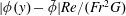 $|\unicode[STIX]{x1D719}(y)-\bar{\unicode[STIX]{x1D719}}|Re/(Fr^{2}G)$
for two representative values of
$|\unicode[STIX]{x1D719}(y)-\bar{\unicode[STIX]{x1D719}}|Re/(Fr^{2}G)$
for two representative values of
 $Re/Fr^{2}$
, over a range of
$Re/Fr^{2}$
, over a range of
 $\bar{\unicode[STIX]{x1D719}}$
and for modest
$\bar{\unicode[STIX]{x1D719}}$
and for modest
 $B$
and
$B$
and
 $n$
. Comparing figures 11(a) and 11(b) reveals that, as expected, the errors are larger as
$n$
. Comparing figures 11(a) and 11(b) reveals that, as expected, the errors are larger as
 $Re/Fr^{2}$
grows. Perhaps surprisingly, for
$Re/Fr^{2}$
grows. Perhaps surprisingly, for
 $Re/Fr^{2}\sim 10$
(figure 11
a) the errors are small, and even for
$Re/Fr^{2}\sim 10$
(figure 11
a) the errors are small, and even for
 $Re/Fr^{2}\sim 60$
(figure 11
b) the errors are less than 10 % for dense suspensions
$Re/Fr^{2}\sim 60$
(figure 11
b) the errors are less than 10 % for dense suspensions
 $(\bar{\unicode[STIX]{x1D719}}\geqslant 40\,\%)$
, which have been the focus of our study (see figures 5–10).
$(\bar{\unicode[STIX]{x1D719}}\geqslant 40\,\%)$
, which have been the focus of our study (see figures 5–10).

Figure 11. Colour maps of
 $|\unicode[STIX]{x1D719}(y)-\bar{\unicode[STIX]{x1D719}}|Re/(Fr^{2}G)$
for a typical inertial fracturing flow with parameters (a)
$|\unicode[STIX]{x1D719}(y)-\bar{\unicode[STIX]{x1D719}}|Re/(Fr^{2}G)$
for a typical inertial fracturing flow with parameters (a)
 $Re=10$
,
$Re=10$
,
 $B=1$
,
$B=1$
,
 $n=0.5$
,
$n=0.5$
,
 $Fr=1$
,
$Fr=1$
,
 $s=2.65$
and
$s=2.65$
and
 $\unicode[STIX]{x1D6FF}_{p}=0.05$
and (b)
$\unicode[STIX]{x1D6FF}_{p}=0.05$
and (b)
 $Re=400$
,
$Re=400$
,
 $B=1$
,
$B=1$
,
 $n=0.5$
,
$n=0.5$
,
 $Fr=2.5$
,
$Fr=2.5$
,
 $s=2.65$
and
$s=2.65$
and
 $\unicode[STIX]{x1D6FF}_{p}=0.05$
.
$\unicode[STIX]{x1D6FF}_{p}=0.05$
.
A number of factors contribute to keeping the errors smaller than might be expected. First, even in the case of a Newtonian fluid, with unit mean velocity through a channel with unit width, the modified pressure gradient is
 $G=24$
. The pressure gradient is now increased by both rheology
$G=24$
. The pressure gradient is now increased by both rheology
 $B$
and by the solids phase (although reduced by shear thinning). The point is that
$B$
and by the solids phase (although reduced by shear thinning). The point is that
 $Re\unicode[STIX]{x1D719}/Fr^{2}\ll 1$
is anyway conservative with respect to the typical pressure gradients encountered. Secondly, we note that the rheological effects combine to influence
$Re\unicode[STIX]{x1D719}/Fr^{2}\ll 1$
is anyway conservative with respect to the typical pressure gradients encountered. Secondly, we note that the rheological effects combine to influence
 $\unicode[STIX]{x1D719}(y)$
in a positive way, i.e.
$\unicode[STIX]{x1D719}(y)$
in a positive way, i.e.
 $\unicode[STIX]{x1D719}(y)$
is more blunt than in a Newtonian suspension, which directly reduces the error
$\unicode[STIX]{x1D719}(y)$
is more blunt than in a Newtonian suspension, which directly reduces the error
 $|\unicode[STIX]{x1D719}(y)-\bar{\unicode[STIX]{x1D719}}|Re/(Fr^{2}G)$
. Two reasons for this are: (i) the velocity profiles and shear rates in shear thinning and yield stress fluids are more plug-like, which influences migration; (ii) as revealed in our model and as confirmed in Dagois-Bohy et al. (Reference Dagois-Bohy, Hormozi, Guazzelli and Pouliquen2015),
$|\unicode[STIX]{x1D719}(y)-\bar{\unicode[STIX]{x1D719}}|Re/(Fr^{2}G)$
. Two reasons for this are: (i) the velocity profiles and shear rates in shear thinning and yield stress fluids are more plug-like, which influences migration; (ii) as revealed in our model and as confirmed in Dagois-Bohy et al. (Reference Dagois-Bohy, Hormozi, Guazzelli and Pouliquen2015),
 $\unicode[STIX]{x1D719}(y)$
approaches a critical value less than the jamming volume fraction at the channel centre. The latter means that
$\unicode[STIX]{x1D719}(y)$
approaches a critical value less than the jamming volume fraction at the channel centre. The latter means that
 $\unicode[STIX]{x1D719}(y)$
must spread more. Note also that in figure 11 we have plotted results with a modest value of
$\unicode[STIX]{x1D719}(y)$
must spread more. Note also that in figure 11 we have plotted results with a modest value of
 $B$
. To conclude, our results suggest that the validity of our leading-order solutions extends beyond
$B$
. To conclude, our results suggest that the validity of our leading-order solutions extends beyond
 $Re\unicode[STIX]{x1D719}/Fr^{2}\ll 1$
to
$Re\unicode[STIX]{x1D719}/Fr^{2}\ll 1$
to
 $Re\unicode[STIX]{x1D719}/Fr^{2}\sim 1$
, and even further depending on the specifics of
$Re\unicode[STIX]{x1D719}/Fr^{2}\sim 1$
, and even further depending on the specifics of
 $\bar{\unicode[STIX]{x1D719}}$
and
$\bar{\unicode[STIX]{x1D719}}$
and
 $B$
. A more detailed study would be required to explore this and other limitations, e.g. particle depletion in wall layers. We note too that examining the errors in the leading-order model is further hampered since in our simplified approach, the two momentum equations in axial and vertical directions are replaced by a single momentum equation along the streamlines. This means that the information about the direction of the main flow is lost. A more comprehensive study of the model error is, however, planned for our future work.
$B$
. A more detailed study would be required to explore this and other limitations, e.g. particle depletion in wall layers. We note too that examining the errors in the leading-order model is further hampered since in our simplified approach, the two momentum equations in axial and vertical directions are replaced by a single momentum equation along the streamlines. This means that the information about the direction of the main flow is lost. A more comprehensive study of the model error is, however, planned for our future work.
Finally, one of the main issues in making the approximation of
 $\unicode[STIX]{x1D719}Re/Fr^{2}$
by
$\unicode[STIX]{x1D719}Re/Fr^{2}$
by
 $\bar{\unicode[STIX]{x1D719}}Re/Fr^{2}$
concerns what has been called ‘slurry convection’, whereby heavier and denser parts of the suspension may fall as a consolidated plug, balanced by an upflow of solids-depleted lighter fluid (closer to the walls). If such a situation occurs, the leading-order solution presented will not be valid (see also Dontsov & Peirce Reference Dontsov and Peirce2014). The point about slurry convection is that the local particle drag, which has relatively small relative velocity, is replaced by a bulk-scale buoyancy-driven motion, which allows for larger relative velocities. However, slurry convection is not well understood. The actual occurrence of slurry convection is not a simple matter of being able to develop a different 1D velocity solution following a different transverse description of the solids distribution. In particular, we should note that bulk exchange flows in pipes and channels frequently do not remain stratified with buoyancy balanced by viscous stresses. The rapid motions induced by buoyancy become balanced by bulk inertial stresses, which leads to mixing, so that model-predicted 1D convection states are not always found in practice.
$\bar{\unicode[STIX]{x1D719}}Re/Fr^{2}$
concerns what has been called ‘slurry convection’, whereby heavier and denser parts of the suspension may fall as a consolidated plug, balanced by an upflow of solids-depleted lighter fluid (closer to the walls). If such a situation occurs, the leading-order solution presented will not be valid (see also Dontsov & Peirce Reference Dontsov and Peirce2014). The point about slurry convection is that the local particle drag, which has relatively small relative velocity, is replaced by a bulk-scale buoyancy-driven motion, which allows for larger relative velocities. However, slurry convection is not well understood. The actual occurrence of slurry convection is not a simple matter of being able to develop a different 1D velocity solution following a different transverse description of the solids distribution. In particular, we should note that bulk exchange flows in pipes and channels frequently do not remain stratified with buoyancy balanced by viscous stresses. The rapid motions induced by buoyancy become balanced by bulk inertial stresses, which leads to mixing, so that model-predicted 1D convection states are not always found in practice.


