

1. Introduction
Multiphase flows with phase transitions and heat transfer are ubiquitous in natural and industrial processes, such as atmospheric phenomena, material and food processing, petrochemical engineering and bio-medicine, as well as life sciences (Brennen Reference Brennen2005; Bernaschi, Melchionna & Succi Reference Bernaschi, Melchionna and Succi2019; Zang et al. Reference Zang, Tarafdar, Tarasevich, Choudhury and Dutta2019; Wu, Liu & Wang Reference Wu, Liu and Wang2021b). Therefore, establishing accurate, reliable and efficient models and computational strategies for predicting their flow behaviour will deepen our understanding of the fundamental and underlying physical mechanisms behind multiphase flows. Besides major academic significance as complex phenomena far from equilibrium, they also bear essential industrial value.
Nevertheless, multi-scale modelling and simulation of such a complex system is a long-standing challenge (Luo, Xia & Monaco Reference Luo, Xia and Monaco2009; Bernaschi et al. Reference Bernaschi, Melchionna and Succi2019; Zang et al. Reference Zang, Tarafdar, Tarasevich, Choudhury and Dutta2019). The challenge arises from the common and unique features of these fluids: (i) complex multi-scale structures and their cross-scale correlations, such as particles, bubbles, droplets and clusters; (ii) rich and abundant evolving interfaces, such as material and mechanical interfaces; (iii) complex forces, relaxations and responses, such as gradient, interparticle and external forces, and the nonlinear coupling among them; (iv) competition between various spatiotemporal scales and kinetic modes, such as growth, deformation, breakup, cavitation, boiling and even turbulence.
In general, a multiphase flow system is in a global or local thermo-hydrodynamic non-equilibrium (THNE) state with fluctuations (Parsa & Wagner Reference Parsa and Wagner2020), including significant hydrodynamic and thermodynamic non-equilibrium (HNE and TNE, respectively) effects that may undermine the validity of macroscopic models, such as the most commonly used Navier–Stokes (NS) equations. Simplifying assumptions, such as thermal equilibrium across a liquid–vapour interface during phase separation, can lead to erroneous predictions (Persad & Ward Reference Persad and Ward2016). A possible solution for accessing detailed THNE effects is to use particle-based methods, for example, molecular dynamics or the direct simulation Monte Carlo method (Liu et al. Reference Liu, Zhang, Kang, Zhang, Duan and He2017, Reference Liu, Zhou, Kang, Zhang, Duan, Zhang and He2020). However, the spatiotemporal scales and geometries that the two schemes can afford are extremely small and highly idealized compared with those of practical applications.
As a mesoscopic approach and a natural bridge connecting microscopic and macroscopic models, suitably extended versions of the Boltzmann equation can in principle describe the complex non-equilibrium thermo-hydrodynamics for the full spectrum of flow regimes (Chapman & Cowling Reference Chapman and Cowling1990). However, the nonlinearity, multi-dimensionality, and integro-differential nature of the collision term pose a formidable challenge to its direct solution. The difficulty in using the original Boltzmann equation has prompted the development of approximate and simplified kinetic models that relinquish much of its computational complexity while preserving its most relevant physics in point. The versatile lattice Boltzmann method (LBM) (Benzi, Succi & Vergassola Reference Benzi, Succi and Vergassola1992; Chen & Doolen Reference Chen and Doolen1998; Wagner & Yeomans Reference Wagner and Yeomans1998; Succi Reference Succi2001, Reference Succi2018; Zheng, Shu & Chew Reference Zheng, Shu and Chew2006; Sbragaglia et al. Reference Sbragaglia, Benzi, Biferale, Succi, Sugiyama and Toschi2007; Xu et al. Reference Xu, Zhang, Gan, Chen and Yu2012; Guo & Shu Reference Guo and Shu2013; Bernaschi et al. Reference Bernaschi, Melchionna and Succi2019; Falcucci et al. Reference Falcucci, Amati, Fanelli, Krastev, Polverino, Porfiri and Succi2021; Huang et al. Reference Huang, Tian, Young and Lai2021a; Bhairapurada, Denet & Boivin Reference Bhairapurada, Denet and Boivin2022; Wei et al. Reference Wei, Li, Wang, Yang, Zhu, Qian and Luo2022) and the recently developed discrete Boltzmann method (DBM) (Gan et al. Reference Gan, Xu, Zhang and Succi2015, Reference Gan, Xu, Zhang, Zhang and Succi2018, Reference Gan, Xu, Zhang, Lin and Liu2019; Lai et al. Reference Lai, Xu, Zhang, Gan, Ying and Succi2016; Lin et al. Reference Lin, Luo, Fei and Succi2017; Zhang et al. Reference Zhang, Xu, Zhang, Gan, Chen and Succi2019, Reference Zhang, Xu, Zhang, Li, Lai and Hu2021; Chen et al. Reference Chen, Xu, Zhang and Zeng2020; Xu et al. Reference Xu, Chen, Song, Chen and Chen2021a,Reference Xu, Shan, Chen, Gan and Linb,Reference Xu, Song, Chen, Xie and Yingc) belong precisely to this class of modern non-equilibrium methods.
As for the LBM research, there are two complementary branches. The first is a physics-inspired construction method, while the second is a numerical scheme for solving partial differential equations, such as the wave equation (Yan Reference Yan2000; Lai & Ma Reference Lai and Ma2011), convection–diffusion equation (Du & Liu Reference Du and Liu2020; Chen et al. Reference Chen, Chai, Shang and Shi2021b), Poisson equation (Chai & Shi Reference Chai and Shi2008), Laplace equation (Zhang, Yan & Dong Reference Zhang, Yan and Dong2009), Fisher equation (Succi Reference Succi2014), Burgers equation (Elton Reference Elton1996; Duan & Liu Reference Duan and Liu2007; Liu & Shi Reference Liu and Shi2011), Benjamin–Ono equation (Lai & Ma Reference Lai and Ma2010), Korteweg–de Vries equation (Wang Reference Wang2017b; Lan, Hu & Guo Reference Lan, Hu and Guo2019), Klein–Gordon–Zakharov equation (Wang Reference Wang2019), Zakharov–Kuznetsov equation (Wang Reference Wang2017a, Reference Wang2020), Ginzburg–Landau equation (Zhang & Yan Reference Zhang and Yan2010, Reference Zhang and Yan2014), Kuramoto–Sivashinsky equation (Otomo, Boghosian & Dubois Reference Otomo, Boghosian and Dubois2018) and Schrödinger equation (Succi Reference Succi2001; He & Lin Reference He and Lin2020). These two branches build on similar, yet not equal, construction rules. The DBM was developed from the first branch and represents a mesoscopic modelling method for fluid flows.
Although the original Boltzmann equation and its approximations work only for dilute gas systems, they can be extended to multiphase flow regimes after incorporating the non-ideal gas effects through a variety of approaches. Actually, both the LBM and the DBM are particularly promising in the area of multiphase and multi-component flows, mainly on account of their kinetic nature, directly inherited from the Boltzmann equation, which facilitates the inclusion of microscopic physical interactions as compared to numerical methods based on continuum models.
To date, many LBMs for multiphase flows have been proposed, including the chromodynamic model Gunstensen et al. (Reference Gunstensen, Rothman, Zaleski and Zanetti1991), the pseudo-potential model (Shan & Chen Reference Shan and Chen1993, Reference Shan and Chen1994), the free-energy model (Swift, Osborn & Yeomans Reference Swift, Osborn and Yeomans1995; Swift et al. Reference Swift, Orlandini, Osborn and Yeomans1996; Xu, Gonnella & Lamura Reference Xu, Gonnella and Lamura2003, Reference Xu, Gonnella and Lamura2004), the kinetic-theory-based model (He, Shan & Doolen Reference He, Shan and Doolen1998; He, Chen & Zhang Reference He, Chen and Zhang1999), the forcing model (Sofonea et al. Reference Sofonea, Lamura, Gonnella and Cristea2004; Gonnella, Lamura & Sofonea Reference Gonnella, Lamura and Sofonea2007), the phase-field model (Rasin, Miller & Succi Reference Rasin, Miller and Succi2005), the entropic kinetic model (Mazloomi M, Chikatamarla & Karlin Reference Mazloomi M, Chikatamarla and Karlin2015; Montessori et al. Reference Montessori, Prestininzi, La Rocca and Succi2017; Wöhrwag et al. Reference Wöhrwag, Semprebon, Mazloomi Moqaddam, Karlin and Kusumaatmaja2018) and the unified collision model (Luo, Fei & Wang Reference Luo, Fei and Wang2021). Although the models are proposed from different perspectives, their common point is the inclusion of interparticle interactions at the mesoscopic scale. The interparticle interactions are the underlying engine behind the complex THNE features of multiphase flows. The aforementioned models and their revised versions have been applied successfully to the study of fundamental phenomena and mechanisms of multiphase flows in science and engineering, ranging from droplet evaporation (Ledesma-Aguilar, Vella & Yeomans Reference Ledesma-Aguilar, Vella and Yeomans2014; Safari, Rahimian & Krafczyk Reference Safari, Rahimian and Krafczyk2014; Zarghami & Van den Akker Reference Zarghami and Van den Akker2017; Qin et al. Reference Qin, Del Carro, Mazloomi Moqaddam, Kang, Brunschwiler, Derome and Carmeliet2019; Fei et al. Reference Fei, Qin, Wang, Luo, Derome and Carmeliet2022) to droplet deformation, breakup, splashing and coalescence (Wagner, Wilson & Cates Reference Wagner, Wilson and Cates2003; Wang et al. Reference Wang, Shu, Huang and Teo2015a; Wang, Shu & Yang Reference Wang, Shu and Yang2015b; Chen & Deng Reference Chen and Deng2017; Wen et al. Reference Wen, Zhou, He, Zhang and Fang2017, Reference Wen, Zhao, Qiu, Ye and Shan2020; Liu et al. Reference Liu, Ba, Wu, Li, Xi and Zhang2018; Liang et al. Reference Liang, Li, Chen and Xu2019; Yang et al. Reference Yang, Liu, Zhuo and Zhong2022b), collapsing cavitation (Chen, Zhong & Yuan Reference Chen, Zhong and Yuan2011; Falcucci et al. Reference Falcucci, Jannelli, Ubertini and Succi2013; Kähler et al. Reference Kähler, Bonelli, Gonnella and Lamura2015; Sofonea et al. Reference Sofonea, Biciuşcă, Busuioc, Ambruş, Gonnella and Lamura2018; Yang et al. Reference Yang, Shan, Kan, Shangguan and Han2020, Reference Yang, Shan, Su, Kan, Shangguan and Han2022a), acoustics levitation (Zang Reference Zang2020), nucleate boiling (Li et al. Reference Li, Luo, Kang, He, Chen and Liu2016, Reference Li, Yu, Zhou and Yan2018; Fei et al. Reference Fei, Yang, Chen, Mo and Luo2020), ferrofluid and electro-hydrodynamic flows (Falcucci et al. Reference Falcucci, Chiatti, Succi, Mohamad and Kuzmin2009; Hu, Li & Niu Reference Hu, Li and Niu2018; Liu, Chai & Shi Reference Liu, Chai and Shi2019), hydrodynamic instability (Zhang et al. Reference Zhang, He, Doolen and Chen2001; Fakhari & Lee Reference Fakhari and Lee2013; Liang et al. Reference Liang, Shi, Guo and Chai2014, Reference Liang, Li, Shi and Chai2016a; Liang, Shi & Chai Reference Liang, Shi and Chai2016b; Yang, Zhong & Zhuo Reference Yang, Zhong and Zhuo2019; Tavares et al. Reference Tavares, Biferale, Sbragaglia and Mailybaev2021), dendritic growth (Rasin et al. Reference Rasin, Miller and Succi2005; Rojas, Takaki & Ohno Reference Rojas, Takaki and Ohno2015; Sun et al. Reference Sun, Pan, Han and Sun2016a,Reference Sun, Zhu, Wang and Sunb), heat and mass transfer in porous media (Chen et al. Reference Chen, Kang, Tang, Robinson, He and Tao2015; Chai et al. Reference Chai, Huang, Shi and Guo2016, Reference Chai, Liang, Du and Shi2019; Liu et al. Reference Liu, Kang, Leonardi, Schmieschek, Narváez, Jones, Williams, Valocchi and Harting2016; He et al. Reference He, Liu, Li and Tao2019), Rayleigh–Bénard convection (Pelusi et al. Reference Pelusi, Sbragaglia, Benzi, Scagliarini, Bernaschi and Succi2021), active fluid (Cates et al. Reference Cates, Fielding, Marenduzzo, Orlandini and Yeomans2008; Doostmohammadi et al. Reference Doostmohammadi, Adamer, Thampi and Yeomans2016; Carenza et al. Reference Carenza, Gonnella, Marenduzzo and Negro2019; Negro et al. Reference Negro, Carenza, Lamura, Tiribocchi and Gonnella2019), isotropic turbulence (Perlekar et al. Reference Perlekar, Benzi, Clercx, Nelson and Toschi2014; Milan et al. Reference Milan, Biferale, Sbragaglia and Toschi2020), solid–liquid–vapour phase transition and phase ordering under various conditions (Osborn et al. Reference Osborn, Orlandini, Swift, Yeomans and Banavar1995; Gonnella, Orlandini & Yeomans Reference Gonnella, Orlandini and Yeomans1997; Corberi, Gonnella & Lamura Reference Corberi, Gonnella and Lamura1998; Kendon et al. Reference Kendon, Desplat, Bladon and Cates1999; Sofonea et al. Reference Sofonea, Lamura, Gonnella and Cristea2004; Gonnella et al. Reference Gonnella, Lamura, Piscitelli and Tiribocchi2010; Coclite, Gonnella & Lamura Reference Coclite, Gonnella and Lamura2014; Wang et al. Reference Wang, Li, Li and Geng2017; Ambruş et al. Reference Ambruş, Busuioc, Wagner, Paillusson and Kusumaatmaja2019; Busuioc et al. Reference Busuioc, Ambruş, Biciuşcă and Sofonea2020; Chen et al. Reference Chen, Shu, Yang, Zhao and Liu2021c; Huang, Wu & Adams Reference Huang, Wu and Adams2021b).
Notwithstanding significant progress, the highly non-equilibrium interfacial thermo- hydrodynamics, which is strongly associated with the growth kinetics and morphological evolution of systems, is seldom reported and still poorly understood. This topic has presented a challenge to the important front of trans-scale modelling and simulation of multiphase flows.
Recently, we have demonstrated that the DBM offers a novel systematic scheme and a set of convenient and efficient tools for describing, measuring and analysing simultaneously THNE effects that cannot be described adequately by traditional hydrodynamic models (Xu et al. Reference Xu, Zhang, Gan, Chen and Yu2012; Gan et al. Reference Gan, Xu, Zhang and Succi2015, Reference Gan, Xu, Zhang, Zhang and Succi2018; Lai et al. Reference Lai, Xu, Zhang, Gan, Ying and Succi2016; Zhang et al. Reference Zhang, Xu, Zhang, Gan, Chen and Succi2019, Reference Zhang, Xu, Zhang, Li, Lai and Hu2021, Reference Zhang, Xu, Zhang, Gan and Li2022a; Chen et al. Reference Chen, Xu, Zhang and Zeng2020, Reference Chen, Xu, Zhang, Gan, Liu and Wang2022a; Liu et al. Reference Liu, Song, Xu, Zhang and Xie2022). The DBM was developed from a branch of the LBM that aims to describe the non-equilibrium flows from a more fundamental level and is no longer based on the simple ‘propagation  $+$ collision’ lattice gas evolution scenario. The key point of the DBM is to ensure that the properties to be studied do not change with model simplification and use the non-conservative kinetic moments of
  $(f-f^{(0)})$ to describe the system state and extract TNE and THNE information (Xu, Zhang & Zhang Reference Xu, Zhang and Zhang2018a; Xu et al. Reference Xu, Chen, Song, Chen and Chen2021a,Reference Xu, Shan, Chen, Gan and Linb,Reference Xu, Song, Chen, Xie and Yingc), where
  $f$ is the distribution function, and
  $f^{(0)}$ is the equilibrium distribution function. Therefore, the simplified Boltzmann-like equation and kinetic moment relations that are not compliant with non-equilibrium statistical physics are prohibited in the DBM. Further, the DBM uses non-conservative kinetic moments of
  $(f-f^{(0)})$ to open a phase space where the origin corresponds to the thermodynamic equilibrium state, and other points correspond to specific THNE states. The phase space and its subspaces provide a graphic geometric description of non-equilibrium states. Evidently, each non-conservative kinetic moment of
  $(f-f^{(0)})$ provides its specific contribution to the overall departure from local equilibrium. Hence, as explained above, the choice of the non-equilibrium moments to be retained is dictated by the specific problem at hand.
Methodologically, the DBM belongs to the general framework of non-equilibrium statistical physics, i.e. a specific form of coarse-graining as applied to the physics of fluids beyond the hydrodynamic level. Specifically, the THNE effects presented by the DBM have permitted us to recover the main features of the distribution function (Lin et al. Reference Lin, Xu, Zhang, Li and Succi2014; Su & Lin Reference Su and Lin2022), to capture various interfacial phenomena (Lin et al. Reference Lin, Xu, Zhang, Li and Succi2014; Lai et al. Reference Lai, Xu, Zhang, Gan, Ying and Succi2016; Gan et al. Reference Gan, Xu, Zhang, Lin and Liu2019), to investigate entropy-increasing mechanisms and their relative importance (Zhang et al. Reference Zhang, Xu, Zhang, Zhu and Lin2016, Reference Zhang, Xu, Zhang, Gan, Chen and Succi2019), and to clarify some of the fundamental mechanisms of the fine structures of shock waves, contact discontinuities and rarefaction waves beyond the reach of molecular dynamics (Gan et al. Reference Gan, Xu, Zhang, Zhang and Succi2018; Qiu et al. Reference Qiu, Bao, Zhou, Che, Chen and You2020, Reference Qiu, Zhou, Bao, Zhou, Che and You2021; Bao et al. Reference Bao, Qiu, Zhou, Zhou, Weng, Lin and You2022). Kinetic features, such as the unbalancing and mutual conversion of internal energy at different degrees of freedom, provide appropriate criteria for determining whether or not higher-order TNE effects should be considered in the modelling, and which level of DBM should be adopted (Lin et al. Reference Lin, Xu, Zhang, Li and Succi2014; Gan et al. Reference Gan, Xu, Zhang and Succi2015, Reference Gan, Xu, Zhang, Zhang and Succi2018). In plasma physics, kinetic features have been used to distinguish plasma shock wave from shock wave in ordinary neutral flow (Liu et al. Reference Liu, Song, Xu, Zhang and Xie2022). These findings and observations shed light on the fundamental mechanisms of various compressible flow systems.
As for the more complicated multiphase case, in 2015, we proposed a DBM with a more realistic equation of state (EOS) to study the HNE and TNE manifestations induced by interparticle and gradient force during phase transition (Gan et al. Reference Gan, Xu, Zhang and Succi2015). We found that the maximum of TNE strength can be used as a physical criterion to discriminate the stages of spinodal decomposition and domain growth. In 2019, we further found that the maximum of entropy production rate can be used as another physical criterion to discriminate the two stages (Zhang et al. Reference Zhang, Xu, Zhang, Gan, Chen and Succi2019), whereas these models are suitable only for cases with weak non-equilibrium effects, or cases in which the Knudsen number is sufficiently small, including phase separation with a slow quenching rate, shallow quenching depth, limited liquid–vapour density ratio, weak viscous stress and heat flux, but wide interface width.
Two prominent reasons account for the insufficiency of the model far from equilibrium. First, constitutive relations are strictly associated with TNE measures, accounting for the coupling of distinct lengths or time scales, and ultimately determining the accuracy of the hydrodynamic model. Given that few kinetic moments are satisfied by the discrete equilibrium distribution function (DEDF), the model in the previous study (Gan et al. Reference Gan, Xu, Zhang and Succi2015) is consistent only with Onuki's model (Onuki Reference Onuki2005, Reference Onuki2007) for Carnahan–Starling fluid in the hydrodynamic limit with linear constitutive relations, that is, Newton's law of viscosity and Fourier's law of heat conduction. Nevertheless, linear constitutive relations result only from the first-order deviation from the thermodynamic equilibrium, and are inadequate for cases with substantial HNE and TNE effects. Second, although higher-order TNE measures and their evolution can be extracted from this DBM (Gan et al. Reference Gan, Xu, Zhang and Succi2015), whether or not they are accurate enough should be carefully estimated, preserved and improved.
In this study, we aim to develop a higher-order DBM for the multi-scale modelling of multiphase flow systems ranging from continuum to transition flow regimes. All the inspiring works on higher-order mesoscopic models for non-equilibrium ideal gas flows (Philippi et al. Reference Philippi, Hegele, dos Santos and Surmas2006; Shan, Yuan & Chen Reference Shan, Yuan and Chen2006; Zhang, Shan & Chen Reference Zhang, Shan and Chen2006; Ansumali et al. Reference Ansumali, Karlin, Arcidiacono, Abbas and Prasianakis2007; Chikatamarla & Karlin Reference Chikatamarla and Karlin2009; Xu Reference Xu2014; Montessori et al. Reference Montessori, Prestininzi, La Rocca and Succi2015; Ambruş & Sofonea Reference Ambruş and Sofonea2016; Coreixas et al. Reference Coreixas, Wissocq, Puigt, Boussuge and Sagaut2017; Yang et al. Reference Yang, Shu, Yang, Chen and Dong2018; Li, Shi & Shan Reference Li, Shi and Shan2019; He et al. Reference He, Tao, Yang, Lu and He2021; Shi & Shan Reference Shi and Shan2021; Shi, Wu & Shan Reference Shi, Wu and Shan2021; Zhang et al. Reference Zhang, Xu, Zhang, Gan and Li2022a) are out of the scope of the present work, although they can be extended into multiphase flow systems with the approaches listed above. Instead, through Chapman–Enskog multi-scale expansion, we first establish the relationships between TNE measures and the generalized constitutive relations for viscous stress and heat flux beyond the Burnett level; we formulate specific expressions with second-order accuracy for viscous stress, heat flux and other higher-order TNE and THNE quantities that are strictly associated with the evolution of constitutive relations. Moreover, we determine all the fewest required kinetic moments that the DEDF should satisfy, and construct three DBMs for multiphase flows near equilibrium and far from equilibrium by inversely solving the required kinetic moments with efficient discrete velocity models. Finally, we demonstrate theoretically and numerically that the capability of the DBM in describing TNE and THNE effects, as well as its multi-scale predictive capability, depends on the kinetic moments specifically recovered by the DEDF.
2. DBM for multiphase flows far from equilibrium
In this section, we first reconsider what the original Boltzmann Bhatnagar–Gross–Krook (BGK) model (Bhatnagar, Gross & Krook Reference Bhatnagar, Gross and Krook1954) describes, and place the BGK model frequently used for various non-equilibrium flows in the proper theoretical perspective for the description of non-dilute systems. Then we focus on the establishment of the links among the Boltzmann–BGK equation, extended hydrodynamic models and THNE phenomena; we determine the necessary kinetic moments to measure THNE effects and discretize phase space using a moment-matching approach. Finally, we present the application of DBMs to multiphase flows far from equilibrium.
2.1. Discrete formulation of density functional kinetic theory
Extended hydrodynamics or generalized hydrodynamics models consider non-equilibrium effects through nonlinear constitutive relations. Correspondingly, high-order kinetic models consider non-equilibrium effects via higher-order distribution functions deviating from equilibrium. As a result, they are expected to be applicable to flows in the slip and transition flow regimes where the NS equations perform poorly (Struchtrup Reference Struchtrup2005; Gao & Sun Reference Gao and Sun2014). A popular strategy for deriving such models is to perform a Chapman–Enskog multi-scale expansion. In a multiphase system, the starting point is the Boltzmann–BGK equation, supplemented by an appropriate interparticle force (Gonnella et al. Reference Gonnella, Lamura and Sofonea2007):
 \begin{equation} \partial_{t}f+\boldsymbol{v} \boldsymbol{\cdot} \boldsymbol{\nabla} f={-}\frac{1}{\tau }[f-f^{(0)}]+I, \end{equation}
where  $f^{(0)}=({\rho }/{2{\rm \pi} T})\exp [-{\boldsymbol {v}^{\ast }\boldsymbol {\cdot } \boldsymbol {v}^{\ast }}/{2T}]$ in the two-dimensional case, with
  $\rho$,
  $T$ and
  $\boldsymbol {v}^{\ast }$ the local density, temperature and thermal velocity, respectively. Here,
  $\boldsymbol {v}^{\ast }=\boldsymbol {v}-\boldsymbol {u}$, with
  $\boldsymbol {v}$ the particle velocity, and
  $\boldsymbol {u}$ the fluid velocity. Finally,
  $I$ indicates the kinetic formulation of interparticle force accounting for the non-ideal gas effects.
At this stage, it is important to point out that the original BGK equation (Bhatnagar et al. Reference Bhatnagar, Gross and Krook1954) assumes that the net effect of collisions is to relax the velocity distribution function towards a local equilibrium distribution  $f^{(0)}$, over a microscopic velocity-independent characteristic timescale
  $\tau$. As a result, it describes molecular collisions in an averaged statistical form, with the only constraint of preserving mass/momentum/energy conservation, as well as the
  $H$-theorem, to secure convergent evolution towards a local equilibrium. Strictly speaking, the BGK model is valid only close to equilibrium, i.e.
  $Kn\ll 1$ and
  $f\simeq f^{(0)}$, thus covering only a very small portion of the full kinetic space.
To study the kinetic behaviour of non-ideal fluids far from equilibrium, one needs to account for interparticle interactions beyond binary collisions, as well as non-equilibrium effects triggered by strong inhomogeneities. This can be achieved by resorting to a mean-field theory formulation (Stanley Reference Stanley1971), or, more precisely, to a density functional kinetic theory (DFKT) (Succi et al. Reference Succi, Montessori, Lauricella, Tiribocchi and Bonaccorso2021). The role of DFKT is twofold: (1) include the effects of the intermolecular interaction potential, omitted by the Boltzmann equation; (2) extend the application scope of the BGK model to non-equilibrium phenomena beyond hydrodynamics. In a pictorial form (see figure 1), one could say that DFKT provides an ‘analytic continuation’ of the BGK model to regions of kinetic phase space not covered by the original Boltzmann equation itself. Here, BGK-like refers to various families of model Boltzmann equations based on single and multi-time relaxation approximations.
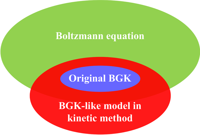
Figure 1. Schematic diagram of the application scopes of the Boltzmann equation, the original BGK model, and a BGK-like model in the kinetic method.
In addition, the BGK-like models used widely in the study of complex fluids include several other physical modelling improvements, for example: relaxation times related to local macroscopic quantities (Li & Zhang Reference Li and Zhang2004; Li et al. Reference Li, Peng, Zhang and Yang2015) and collision frequency (Struchtrup Reference Struchtrup1997); pseudo-equilibrium distribution functions that contain non-equilibrium information (Holway Reference Holway1966; Shakhov Reference Shakhov1968; Shan et al. Reference Shan, Yuan and Chen2006; Gao & Sun Reference Gao and Sun2014; Watari Reference Watari2016); internal degrees of freedom (Rykov Reference Rykov1975) and even quantum vibrational energy (Wu et al. Reference Wu, Li, Zhang and Peng2021a); and appropriate kinetic boundary conditions (Wagner & Pagonabarraga Reference Wagner and Pagonabarraga2002; Sbragaglia & Succi Reference Sbragaglia and Succi2005; Sofonea & Sekerka Reference Sofonea and Sekerka2005; Toschi & Succi Reference Toschi and Succi2005; Benzi et al. Reference Benzi, Biferale, Sbragaglia, Succi and Toschi2006; Chikatamarla, Ansumali & Karlin Reference Chikatamarla, Ansumali and Karlin2006; Chen, Zhang & Zhang Reference Chen, Zhang and Zhang2013). These improved models permit to capture a wider range of Knudsen numbers and a higher degree of non-equilibrium.
The multi-scale multiphase DFKT is expected to contribute to the area of materials science for energy–environment applications (Succi et al. Reference Succi, Amati, Bonaccorso, Lauricella, Bernaschi, Montessori and Tiribocchi2020) and medical purposes (Xu et al. Reference Xu, Wang, Liu, Tang and Tian2018b; Li et al. Reference Li, Luo, Liu, Xu, Tian and Wang2022). For instance, it may help us: to understand the non-equilibrium transport processes of multiphase flow in proton exchange membrane fuel cells for obtaining better performance, and lower cost, emission and noise (Chen, Kang & Tao Reference Chen, Kang and Tao2021a); to investigate the non-equilibrium nucleate boiling mechanism and design suitable surface structures for enhancing nucleate boiling heat transfer efficiency (Biferale et al. Reference Biferale, Perlekar, Sbragaglia and Toschi2012; Li et al. Reference Li, Yu, Zhou and Yan2018, Reference Li, Li, Yu and Wen2020; Fei et al. Reference Fei, Yang, Chen, Mo and Luo2020); to optimize heat source location (Dai et al. Reference Dai, Li, Mostaghimi, Wang and Zeng2020) and improve the latent heat thermal energy storage rate (Ren Reference Ren2019; Tian et al. Reference Tian2022); to conduct mesoscale simulations of blood flow (Dupin, Halliday & Care Reference Dupin, Halliday and Care2006; Yan et al. Reference Yan, Cai, Liu and Fu2012), and generation, transmission and diffusion of bioaerosols (He et al. Reference He, Qin, Chen and Wen2022).
In the present paper, as a specific example of DFKT, the mean-field force  $I$ takes the following form for a liquid–vapour system:
 \begin{equation} I={-}[A+\boldsymbol{B}\boldsymbol{\cdot} \boldsymbol{v}^{{\ast} }+(C+C_{q})\boldsymbol{v}^{{\ast} }\boldsymbol{\cdot} \boldsymbol{v}^{{\ast} }]f^{(0)}. \end{equation}
The coefficients in (2.2) are designed so as to recover the thermo-hydrodynamic equations proposed by Onuki (Onuki Reference Onuki2005) by using the following contributions of the force term  $I$ to mass, momentum and energy equations at the second order in Knudsen number:
 $$\begin{gather} \int_{-\infty }^{\infty } I\,{\rm d}\boldsymbol{v}=A+2(C+C_{q})T, \end{gather}$$
 $$\begin{gather}\int_{-\infty }^{\infty } I\boldsymbol{v}\, {\rm d} \boldsymbol{v}={-}\rho T\boldsymbol{B}, \end{gather}$$
 $$\begin{gather}\int_{-\infty }^{\infty } I\,\frac{\boldsymbol{v}\boldsymbol{\cdot} \boldsymbol{v}}{2}\, {\rm d} \boldsymbol{v}={-}2\rho T^{2}(C+C_{q})-\rho T\boldsymbol{B}\boldsymbol{\cdot} \boldsymbol{u}. \end{gather}$$
As a result,  $A=-2(C+C_{q})T$, indicates that the forcing term guarantees mass conservation, and
  $\boldsymbol {B}=({1}/{\rho T})[\boldsymbol {\nabla }(P^{{CS}}-\rho T)+\boldsymbol {\nabla }\boldsymbol {\cdot } \boldsymbol {\varLambda }]$ describes two contributions of
  $I$ to the fluid momentum. One comes from the difference between the non-ideal gas EOS and the ideal gas EOS, and the other comes from the contribution of density gradient to pressure tensor
  $\boldsymbol {\varLambda }=K\,\boldsymbol {\nabla }\rho \, \boldsymbol {\nabla }\rho -K(\rho \,\nabla ^{2}\rho +\vert \boldsymbol {\nabla }\rho \vert ^{2}/2)\boldsymbol {I}-[\rho T\,\boldsymbol {\nabla }\rho \boldsymbol {\cdot } \boldsymbol {\nabla }(K/T)]\boldsymbol {I}$, with
  $\boldsymbol {I}$ the unit tensor, and
  $K$ the surface tension coefficient. Here, we choose the Carnahan–Starling EOS (Carnahan & Starling Reference Carnahan and Starling1969) as the non-ideal one,
  $P^{{CS}}=\rho T(({1+\eta +\eta ^{2}-\eta ^{3}})/{(1-\eta )^{3}})-a\rho ^{2}$ with
  $\eta =b\rho /4$, which offers a more accurate representation for hard sphere interactions than the van der Waals EOS. A more realistic EOS, such as the Redlich–Kwong (Redlich & Kwong Reference Redlich and Kwong1949) or the Peng–Robinson (Peng & Robinson Reference Peng and Robinson1976), could be incorporated conveniently into the DBM through modifying the extra force term
  $I$ for modelling improvement. Here,
  $C=({1}/{2\rho T^{2}}) \{(P^{CS}-\rho T)\boldsymbol {\nabla }\boldsymbol {\cdot } \boldsymbol {u}+{\boldsymbol {\varLambda }}: \boldsymbol {\nabla } \boldsymbol {u}+a\rho ^{2}\,\boldsymbol {\nabla }\boldsymbol \cdot$
  $\boldsymbol {u}+K[-\frac {1}{2}(\boldsymbol {\nabla } \rho \boldsymbol {\cdot } \boldsymbol {\nabla }\rho )\boldsymbol {\nabla }\boldsymbol {\cdot } \boldsymbol {u}-\rho \, \boldsymbol {\nabla }\rho \boldsymbol {\cdot } \boldsymbol {\nabla }(\boldsymbol {\nabla }\boldsymbol {\cdot } \boldsymbol {u})-\boldsymbol {\nabla }\rho \boldsymbol {\cdot } \boldsymbol {\nabla }\boldsymbol {u}\boldsymbol {\cdot } \boldsymbol {\nabla }\rho ]\}$ represents a partial contribution of
  $I$ to energy. The term
  $C_{q}=({1}/{2\rho T^{2}})\,\boldsymbol {\nabla }\boldsymbol {\cdot } \lbrack 2q\rho T\,\boldsymbol {\nabla }T]$ permits us to tune the heat conductivity independently of the dynamic viscosity (non-unit Prandtl number).
Constructing the density, momentum and energy kinetic moments of (2.1) and recomposing the time derivative, results in the following extended hydrodynamics equations:
 $$\begin{gather} \partial _{t}\rho +\boldsymbol{\nabla}\boldsymbol{\cdot} (\rho \boldsymbol{u})=0, \end{gather}$$
 $$\begin{gather}\partial _{t}(\rho \boldsymbol{u})+\boldsymbol{\nabla}\boldsymbol{\cdot} (\rho \boldsymbol{uu}+\boldsymbol{ \varPi }+\boldsymbol{\varDelta}_{2})=0, \end{gather}$$
 $$\begin{gather}\partial _{t}e_{T}+\boldsymbol{\nabla}\boldsymbol{\cdot} \lbrack e_{T} \boldsymbol{u}+\boldsymbol{\varPi}\boldsymbol{\cdot} \boldsymbol{u}+\boldsymbol{\varDelta}_{3,1}+\kappa_{2}\, \boldsymbol{\nabla}T]=0, \end{gather}$$
where  $\boldsymbol {\varPi }=P^{{CS}}\boldsymbol {I}+\boldsymbol {\varLambda }$ is the non-viscous stress,
  $e_{T}=\rho T-a\rho ^{2}+K\,|\boldsymbol {\nabla }\rho |^{2}/2+\rho u^{2}/2$ is the total energy density, and
  $\kappa _{2}=2\rho Tq$ is an additional heat conductivity originated from
  $C_{q}$ and designed to tune the Prandtl number. Also,
  $\boldsymbol {\varDelta }_{2}$ and
  $\boldsymbol {\varDelta }_{3,1}$ are typical non-equilibrium measures related to the generalized constitutive relations.
Without loss of generality, two sets of non-equilibrium measures can be defined (Xu et al. Reference Xu, Zhang, Gan, Chen and Yu2012; Gan et al. Reference Gan, Xu, Zhang and Succi2015):
 $$\begin{align} \boldsymbol{\varDelta}_{m,n}&=\boldsymbol{M}_{m,n}(f-f^{(0)})=\int_{-\infty }^{\infty } \left(\frac{1}{2}\right)^{1-\delta _{m,n}}(f^{(1)}+f^{(2)}+\cdots){\underbrace{{\boldsymbol{v}\boldsymbol{v}}\cdots {\boldsymbol{v}}} _{n}(\boldsymbol{v}\boldsymbol{\cdot} \boldsymbol{v})}^{({m-n})/{2}}\, {\rm d} \boldsymbol{v}, \end{align}$$
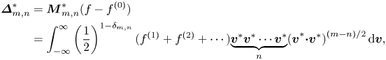 $$\begin{align}\boldsymbol{\varDelta}_{m,n}^{{\ast} }&=\boldsymbol{M}_{m,n}^{{\ast} }(f-f^{(0)})\nonumber\\&=\int_{-\infty }^{\infty } \left(\frac{1}{ 2}\right)^{1-\delta _{m,n}}(f^{(1)}+f^{(2)}+\cdots){\underbrace{{\boldsymbol{v}}^{{\ast} }{ \boldsymbol{v}}^{{\ast} }\cdots {\boldsymbol{v}}^{{\ast} }}_{n}(\boldsymbol{v}}^{{\ast} }{ \boldsymbol{\cdot}\boldsymbol{v}}^{{\ast} }{)}^{({m-n})/{2}}\, {\rm d} \boldsymbol{v}, \end{align}$$
where  $\boldsymbol {\varDelta }_{m,n}$ and
  $\boldsymbol {\varDelta }_{m,n}^{\ast }$ are the
  $m$th-order tensors contracted to
  $n$th-order ones, and
  $\delta _{m,n}$ is the Kronecker delta function. Here,
  $(m-n)/2$ is an integer, and when
  $m=n$,
  $\boldsymbol {\varDelta }_{m,n}$ and
  $\boldsymbol {\varDelta } _{m,n}^{\ast }$ are referred to simplistically as
  $\boldsymbol {\varDelta }_{m}$ and
  $\boldsymbol {\varDelta }_{m}^{\ast }$, respectively. Also,
  $\boldsymbol {\varDelta }_{m,n}$ describes the combination effects of HNE and TNE, which are usually called the thermo-hydrodynamic non-equilibrium (THNE) effects, and
  $\boldsymbol {\varDelta }_{m,n}^{\ast }$ reflects molecular individualism on top of organized collective motion, describing only the TNE effects;
  $\boldsymbol {\varDelta }_{m,n}-\boldsymbol {\varDelta }_{m,n}^{\ast }$ depicts the HNE effects, as a supplemental description of macroscopic quantity gradients. Term
  $\boldsymbol {M}_{m,n}$ (
 $\boldsymbol {M}_{m,n}^{\ast }$) is the non-central (central) kinetic moment, and
  $f^{(\kern0.06em j)}$ represents the
  $\kern0.06em j$th-order derivation from
  $f^{(0)}$. The decomposition relations among THNE and TNE measures are derived and displayed in Appendix A:
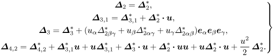 \begin{equation} \left.\begin{array}{c@{}}
\boldsymbol{\varDelta}_{2}=\boldsymbol{\varDelta}_{2}^{{\ast}
}, \\[3pt]
\boldsymbol{\varDelta}_{3,1}=\boldsymbol{\varDelta}_{3,1}^{{\ast}
}+\boldsymbol{\varDelta}_{2}^{{\ast} }\boldsymbol{\cdot}
{\boldsymbol{u}}, \\[3pt]
\boldsymbol{\varDelta}_{3}=\boldsymbol{\varDelta}_{3}^{{\ast}
}+(u_{\alpha }\varDelta_{2\beta \gamma }^{{\ast} }+u_{\beta
}\varDelta_{2\alpha \gamma }^{{\ast} }+u_{\gamma
}\varDelta_{2\alpha \beta }^{{\ast}
})\boldsymbol{e}_{\alpha }\boldsymbol{e}_{\beta
}\boldsymbol{e}_{\gamma }, \\
\boldsymbol{\varDelta}_{4,2}=\boldsymbol{\varDelta}_{4,2}^{{\ast}
}+\boldsymbol{\varDelta}_{3,1}^{{\ast} }
\boldsymbol{u}+\boldsymbol{u}\boldsymbol{\varDelta}_{3,1}^{{\ast}
}+\boldsymbol{\varDelta}_{3}^{{\ast} }\boldsymbol{\cdot}
{\boldsymbol{ u}}+\boldsymbol{\varDelta}_{2}^{{\ast}
}\boldsymbol{\cdot}
{\boldsymbol{uu}}+\boldsymbol{u}\boldsymbol{\varDelta}_{2}^{{\ast}
}\boldsymbol{\cdot}
{\boldsymbol{u}}+\dfrac{u^{2}}{2}\,\boldsymbol{\varDelta}_{2}^{{\ast}
}.
\end{array}\right\}\end{equation}
\begin{equation} \left.\begin{array}{c@{}}
\boldsymbol{\varDelta}_{2}=\boldsymbol{\varDelta}_{2}^{{\ast}
}, \\[3pt]
\boldsymbol{\varDelta}_{3,1}=\boldsymbol{\varDelta}_{3,1}^{{\ast}
}+\boldsymbol{\varDelta}_{2}^{{\ast} }\boldsymbol{\cdot}
{\boldsymbol{u}}, \\[3pt]
\boldsymbol{\varDelta}_{3}=\boldsymbol{\varDelta}_{3}^{{\ast}
}+(u_{\alpha }\varDelta_{2\beta \gamma }^{{\ast} }+u_{\beta
}\varDelta_{2\alpha \gamma }^{{\ast} }+u_{\gamma
}\varDelta_{2\alpha \beta }^{{\ast}
})\boldsymbol{e}_{\alpha }\boldsymbol{e}_{\beta
}\boldsymbol{e}_{\gamma }, \\
\boldsymbol{\varDelta}_{4,2}=\boldsymbol{\varDelta}_{4,2}^{{\ast}
}+\boldsymbol{\varDelta}_{3,1}^{{\ast} }
\boldsymbol{u}+\boldsymbol{u}\boldsymbol{\varDelta}_{3,1}^{{\ast}
}+\boldsymbol{\varDelta}_{3}^{{\ast} }\boldsymbol{\cdot}
{\boldsymbol{ u}}+\boldsymbol{\varDelta}_{2}^{{\ast}
}\boldsymbol{\cdot}
{\boldsymbol{uu}}+\boldsymbol{u}\boldsymbol{\varDelta}_{2}^{{\ast}
}\boldsymbol{\cdot}
{\boldsymbol{u}}+\dfrac{u^{2}}{2}\,\boldsymbol{\varDelta}_{2}^{{\ast}
}.
\end{array}\right\}\end{equation}
Here,  $\boldsymbol {\varDelta }_{2}^{\ast }$ and
  $\boldsymbol {\varDelta }_{3,1}^{\ast }$ are also referred to as the non-organized moment flux (NOMF) and non-organized energy flux (NOEF), respectively. Compared with the NS and Burnett equations,
  $\boldsymbol {\varDelta } _{2}^{\ast }$ and
  $\boldsymbol {\varDelta }_{3,1}^{\ast }$ correspond to more generalized viscous stress and heat flux, which contain all hierarchical TNE effects induced by
  $(f-f^{(0)})$, instead of only
  $f^{(1)}$ at the NS level and
  $f^{(1)}+f^{(2)}$ at the Burnett level. The links among the Boltzmann equation, the extended hydrodynamic equations and TNE measures have been established so far. Terms
  $\boldsymbol {\varDelta }_{3}^{\ast }$ and
  $\boldsymbol {\varDelta }_{4,2}^{\ast }$ are the flux of viscous stress and the flux of heat flux, respectively.
However,  $\boldsymbol {\varDelta }_{2}^{\ast }$ and
  $\boldsymbol {\varDelta }_{3,1}^{\ast }$ are primarily unknown. To obtain the explicit constitutive relations, we perform Chapman–Enskog expansion on both sides of (2.1) by introducing expansions
 $$\begin{gather} f=f^{(0)}+f^{(1)}+f^{(2)}+\cdots, \end{gather}$$
 $$\begin{gather}\partial _{t}=\partial _{t_{1}}+\partial _{t_{2}}+\cdots, \end{gather}$$
 $$\begin{gather}\boldsymbol{\nabla}=\boldsymbol{\nabla}_{1}, \quad I=I_{1}, \end{gather}$$
where  $\partial _{t_{j}}$,
  $\boldsymbol {\nabla }_{j}$ and
  $I_{j}$ are
  $j$th-order terms in Knudsen number
  $\epsilon$. Substituting (2.12)–(2.14) into (2.1), and equating terms that have the same orders in
  $\epsilon$, gives
 $$\begin{gather} \epsilon ^{1}:{\partial }_{t_{1}}{f^{(0)}}+\boldsymbol{\nabla}_{1}\boldsymbol{\cdot} (f^{(0)}\boldsymbol{v})={-}\frac{1}{\tau }\,f^{{(1)}}+I_{1}, \end{gather}$$
 $$\begin{gather}\epsilon ^{2}:{\partial }_{t_{2}}{f^{(0)}}+{\partial }_{t_{1}}{f^{(1)}}+ \boldsymbol{\nabla}_{1}\boldsymbol{\cdot} (f^{(1)}\boldsymbol{v})={-}\frac{1}{\tau }\,f^{{(2)}}. \end{gather}$$
Performing the velocity moments with the collision invariant vector  $(1, \boldsymbol {v}, {v^{2}}/{2})$ on the two sides of (2.15) leads to the following useful relations between the temporal derivative
  $\partial _{t_{1}}$ and the spatial derivative
  $\boldsymbol {\nabla }_{1}$ at
  $\epsilon ^{1}$ level:
 $$\begin{gather} {\partial }_{t_{1}}\rho ={-}\boldsymbol{\nabla}_{1}\boldsymbol{\cdot} (\rho \boldsymbol{u}), \end{gather}$$
 $$\begin{gather}{\partial }_{t_{1}}\boldsymbol{u}={-}T\boldsymbol{B}- \boldsymbol{\nabla}_{1}T-\frac{T}{\rho }\, \boldsymbol{\nabla}_{1}\rho -\boldsymbol{u}\boldsymbol{\cdot} \boldsymbol{\nabla}_{1}\boldsymbol{u}, \end{gather}$$
 $$\begin{gather}{\partial }_{t_{1}}T={-}2(C+C_{q})T^{2}-T\,\boldsymbol{\nabla}_{1}\boldsymbol{\cdot} \boldsymbol{u}-\boldsymbol{u}\boldsymbol{\cdot} \boldsymbol{\nabla}_{1}T. \end{gather}$$
From (2.15), we can obtain  $f^{{(1)}}=-\tau \lbrack {\partial }_{t_{1}}f{^{(0)}}+\boldsymbol {\nabla } _{1}\boldsymbol {\cdot } (f^{(0)}\boldsymbol {v})-I_{1}]$. Using (2.17)–(2.19), and after some straightforward but rather tedious algebraic manipulation, we acquire the following relations between thermodynamic forces and fluxes:
 $$\begin{gather} \boldsymbol{\varDelta}_{2}^{{\ast} (1)}=\int_{-\infty }^{\infty } f^{(1)}\boldsymbol{v}^{{\ast} }\boldsymbol{v}^{{\ast} }\, {\rm d} \boldsymbol{v}={-}\mu \lbrack \boldsymbol{\nabla}\boldsymbol{u}+(\boldsymbol{\nabla}\boldsymbol{u})^{\rm T}- \boldsymbol{I}\boldsymbol{\nabla}\boldsymbol{\cdot} \boldsymbol{u}], \end{gather}$$
 $$\begin{gather}\boldsymbol{\varDelta}_{3,1}^{{\ast} (1)}=\int_{-\infty }^{\infty } \frac{1}{2}\,f^{(1)}\boldsymbol{v}^{{\ast} }\boldsymbol{\cdot} \boldsymbol{v}^{{\ast} }\boldsymbol{v}^{{\ast} }\, {\rm d} \boldsymbol{v}={-}\kappa _{1}\,\boldsymbol{\nabla}T. \end{gather}$$
Equations (2.20) and (2.21) indicate that the first orders of NOMF and NOEF are exactly the viscous stress tensor and the heat flux at the NS level, respectively;  $\mu =\rho T\tau$ is the viscosity coefficient, and
  $\kappa _{1}=2\rho T\tau$ is the heat conductivity. Similarly, we have
 $$\begin{gather} \boldsymbol{\varDelta}_{3}^{{\ast} (1)}=\int_{-\infty }^{\infty }f^{(1)}{\boldsymbol{v}} ^{{\ast} }{\boldsymbol{v}}^{{\ast} }{\boldsymbol{v}}^{{\ast} }\, {\rm d} \boldsymbol{v}={-}\rho T\tau (\partial _{\alpha }T\delta _{\beta \gamma }+\partial _{\beta }T\delta _{\alpha \gamma }+\partial _{\gamma }T\delta _{\alpha \beta })\boldsymbol{e} _{\alpha }\boldsymbol{e}_{\beta }\boldsymbol{e}_{\gamma }, \end{gather}$$
 $$\begin{gather}\boldsymbol{\varDelta}_{4,2}^{{\ast} (1)}=\int_{-\infty }^{\infty }f^{(1)}{\boldsymbol{v}} ^{{\ast} }{\boldsymbol{v}}^{{\ast} }\,\frac{{\boldsymbol{v}}^{{\ast} }\boldsymbol{\cdot} {\boldsymbol{v}} ^{{\ast} }}{2}\, {\rm d} \boldsymbol{v}={-}3\rho T^{2}\tau \lbrack \boldsymbol{\nabla}\boldsymbol{u}+( \boldsymbol{\nabla}\boldsymbol{u})^{\rm T}-\boldsymbol{I}\,\boldsymbol{\nabla}\boldsymbol{\cdot} \boldsymbol{u}]. \end{gather}$$
 Deeper TNE effects can be accessed by considering the contributions of  $f^{(2)}$, and clarifying relations between
  $\partial _{t_{2}}$ and
  $\boldsymbol {\nabla }_{1}$ at
  $\epsilon ^{2}$ level according to procedures similar to those listed in (2.17)–(2.19). Specifically, from (2.16), we acquire
 \begin{align} f^{{(2)}} &={-}\tau
\lbrack {\partial }_{t_{2}}f{^{(0)}}+{\partial }_{t_{1}}f{
^{(1)}}+\boldsymbol{\nabla}_{1}\boldsymbol{\cdot}
(f^{(1)}\boldsymbol{v})]\nonumber\\
&={-}\tau\,{\partial
}_{t_{2}}f{^{(0)}}+\tau {^2}\,{\partial
}_{t_{1}}^{2}f{ ^{(0)}}+\tau {^2}\,{\partial
}_{t_{1}}[\boldsymbol{\nabla}_{1}\boldsymbol{\cdot}
(f^{(0)}\boldsymbol{v})]-\tau {^2}\,{\partial
}_{t_{1}}I_{1} \nonumber\\ & \quad +\tau
^{2}\boldsymbol{\nabla}_{1}\boldsymbol{\cdot} \lbrack
{\partial }_{t_{1}}f{^{(0)}}\boldsymbol{
v}+\boldsymbol{\nabla}_{1}\boldsymbol{\cdot}
(f^{(0)}\boldsymbol{vv})-I_{1}\boldsymbol{v}].
\end{align}
\begin{align} f^{{(2)}} &={-}\tau
\lbrack {\partial }_{t_{2}}f{^{(0)}}+{\partial }_{t_{1}}f{
^{(1)}}+\boldsymbol{\nabla}_{1}\boldsymbol{\cdot}
(f^{(1)}\boldsymbol{v})]\nonumber\\
&={-}\tau\,{\partial
}_{t_{2}}f{^{(0)}}+\tau {^2}\,{\partial
}_{t_{1}}^{2}f{ ^{(0)}}+\tau {^2}\,{\partial
}_{t_{1}}[\boldsymbol{\nabla}_{1}\boldsymbol{\cdot}
(f^{(0)}\boldsymbol{v})]-\tau {^2}\,{\partial
}_{t_{1}}I_{1} \nonumber\\ & \quad +\tau
^{2}\boldsymbol{\nabla}_{1}\boldsymbol{\cdot} \lbrack
{\partial }_{t_{1}}f{^{(0)}}\boldsymbol{
v}+\boldsymbol{\nabla}_{1}\boldsymbol{\cdot}
(f^{(0)}\boldsymbol{vv})-I_{1}\boldsymbol{v}].
\end{align}
It is clear that  $f^{(2)}$ can also be expressed in terms of
  $f^{(0)}$. As a result, non-conservative non-equilibrium moments can finally resort to those of
  $f^{(0)}$, which triggers the requirement of the higher-order kinetic moments of
  $f^{(0)}$. The second-order non-organized moment flux reads
 \begin{equation} \boldsymbol{\varDelta}_{2}^{{\ast} (2)}=\boldsymbol{M}_{2}^{{\ast} }(f^{(2)})=\int_{-\infty }^{\infty }f^{(2)}{\boldsymbol{v}}^{{\ast} }{\boldsymbol{v}}^{{\ast} }\, {\rm d} \boldsymbol{v}. \end{equation}
To obtain an explicit expression, relations between  $\partial _{t_{2}}$ and
  $\boldsymbol {\nabla }_{1}$ at
  $\epsilon ^{2}$ level should be clarified. Performing the velocity moments with the collision invariant vector
  $(1, \boldsymbol {v}, {v^{2}}/{2})$ on the two sides of (2.16) leads to the following useful relations between the temporal derivative
  $\partial _{t_{2}}$ and the spatial derivative
  $\boldsymbol {\nabla }_{1}$ at
  $\epsilon ^{2}$ level:
 $$\begin{gather} {\partial }_{t_{2}}\rho =0, \end{gather}$$
 $$\begin{gather}\rho\,{\partial }_{t_{2}}\boldsymbol{u}={-}\boldsymbol{\nabla}_{1}\boldsymbol{\cdot} \boldsymbol{\varDelta}_{2}^{(1)}, \end{gather}$$
 $$\begin{gather}{\partial }_{t_{2}}(\rho T+\tfrac{1}{2}\rho u^{2})={-}\boldsymbol{\nabla}_{1}\boldsymbol{\cdot} \boldsymbol{\varDelta}_{3,1}^{(1)}. \end{gather}$$
Using (2.26)–(2.28) to replace the temporal derivative  $\partial _{t_{2}}$ by spatial derivative
  $\boldsymbol {\nabla }_{1}$ at
  $\epsilon ^{2}$ level, and after some laborious algebraic manipulation, we acquire expression for
  $\boldsymbol {\varDelta }_{2}^{\ast (2)}$. Likewise, analytical expressions for
  $\boldsymbol {\varDelta }_{3,1}^{\ast (2)}$,
  $\boldsymbol {\varDelta }_{3}^{\ast (2)}$ and
  $\boldsymbol {\varDelta }_{4,2}^{\ast (2)}$ can be obtained, as illustrated in Appendix B. The derivation of these expressions is a tough task, so we resort to the software Maple 18.
Furthermore, multiplying (2.1) by  $\boldsymbol {v}^{\ast }\boldsymbol {v} ^{\ast }$ and
  $\frac {1}{2}\boldsymbol {v}^{\ast }\boldsymbol {\cdot } \boldsymbol {v}^{\ast }\boldsymbol {v }^{\ast }$, and integrating over the whole velocity space, we obtain the time-evolution equations for viscous stress and heat flux:
 $$\begin{align} &{\partial }_{t}\boldsymbol{\varDelta}_{2}^{{\ast} }+{\partial }_{t}\boldsymbol{M}_{2}^{{\ast} }(f^{(0)})+\boldsymbol{\nabla}\boldsymbol{\cdot} \lbrack \boldsymbol{M}_{3}^{{\ast} }(f^{(0)})+\boldsymbol{M }_{2}^{{\ast} }(f^{(0)})\boldsymbol{u}+\boldsymbol{\varDelta}_{3}^{{\ast} }+\boldsymbol{\varDelta } _{2}^{{\ast} }\boldsymbol{u}]={-}\frac{1}{\tau }\,\boldsymbol{\varDelta}_{2}^{{\ast} }+\boldsymbol{M} _{2}^{{\ast} }(I), \end{align}$$
 $$\begin{align} &{\partial }_{t}\boldsymbol{\varDelta}_{3,1}^{{\ast} }+{\partial }_{t}\boldsymbol{M} _{3,1}^{{\ast} }(f^{(0)})+\boldsymbol{\nabla}\boldsymbol{\cdot} \lbrack \boldsymbol{M}_{4,2}^{{\ast} }(f^{(0)})+\boldsymbol{M}_{3,1}^{{\ast} }(f^{(0)})\boldsymbol{u}+\boldsymbol{\varDelta } _{4,2}^{{\ast} }+\boldsymbol{\varDelta}_{3,1}^{{\ast} }\boldsymbol{u}]\nonumber\\&\quad={-}\frac{1}{\tau }\, \boldsymbol{\varDelta}_{3,1}^{{\ast} }+\boldsymbol{M}_{3,1}^{{\ast} }(I). \end{align}$$
Equations (2.29) and (2.30) suggest that obtaining the expressions of higher-order TNE quantities, such as  $\boldsymbol {\varDelta }_{3}^{\ast }$ and
  $\boldsymbol {\varDelta }_{4,2}^{\ast }$, enhances our understanding of the evolution mechanisms of nonlinear constitutive relations.
To summarize, higher-order constitutive relations of second-order accuracy for viscous stress and heat transfer can be formulated as  $\boldsymbol {\varDelta }_{2}^{\ast }=\boldsymbol {\varDelta }_{2}^{\ast (1)}+\boldsymbol {\varDelta } _{2}^{\ast (2)}$,
  $\boldsymbol {\varDelta }_{3,1}^{\ast }=\boldsymbol {\varDelta }_{3,1}^{\ast (1)}+ \boldsymbol {\varDelta }_{3,1}^{\ast (2)}$, which are expected to noticeably improve the macroscopic modelling. Meanwhile, higher-order TNE measures with second-order accuracy,
  $\boldsymbol {\varDelta }_{3}^{\ast }=\boldsymbol {\varDelta }_{3}^{\ast (1)}+\boldsymbol {\varDelta }_{3}^{\ast (2)}$,
  $\boldsymbol {\varDelta }_{4,2}^{\ast }=\boldsymbol {\varDelta }_{4,2}^{\ast (1)}+\boldsymbol {\varDelta } _{4,2}^{\ast (2)}$, offer more abundant non-equilibrium scenarios from different aspects and are useful in elucidating the evolutions of higher-order constitutive relations.
In fact, the theoretical expressions of  $\boldsymbol {\varDelta }_{3}^{\ast }$ and
  $\boldsymbol {\varDelta }_{4,2}^{\ast }$ are also constitutive relations, which are omitted in the NS equations. In the case of quasi-continuous and near-equilibrium, it is not a big problem if they are omitted. However, as the degree of discretization and thermodynamic non-equilibrium increase, ignoring
  $\boldsymbol {\varDelta }_{3}^{\ast }$ and
  $\boldsymbol {\varDelta }_{4,2}^{\ast }$ leads to substantial errors. Furthermore, the analytical expressions for THNE with second-order accuracy,
  $\boldsymbol {\varDelta }_{2}=\boldsymbol {\varDelta }_{2}^{(1)}+\boldsymbol {\varDelta }_{2}^{(2)}$,
  $\boldsymbol {\varDelta }_{3,1}=\boldsymbol {\varDelta }_{3,1}^{(1)}+\boldsymbol {\varDelta }_{3,1}^{(2)}$,
  $\boldsymbol {\varDelta }_{3}=\boldsymbol {\varDelta }_{3,1}^{(1)}+\boldsymbol {\varDelta }_{3,1}^{(2)}$ and
  $\boldsymbol {\varDelta }_{4,2}=\boldsymbol {\varDelta }_{4,2}^{(1)}+\boldsymbol {\varDelta }_{4,2}^{(2)}$, can be acquired from (2.11).
2.2. Discretization of particle velocity space
The velocity space discretization is a critical step in DBM modelling. The above expressions for TNE measures (see Appendix B) have been derived from (2.1) with a continuous equilibrium distribution function  $f^{(0)}$. To conduct numerical simulation, it is required to construct a discrete velocity model (DVM)
  $\boldsymbol {v}_{i}$ to discretize the particle velocity space, and formulate the DEDF
  $f_{i}^{(0)}$ satisfying all the needed kinetic moments, where
  $i=1,2,3,\ldots,N$, with
  $N$ the total number of discrete velocities. Chapman–Enskog analysis demonstrates that
  $f_{i}^{(0)}$ should satisfy the seven kinetic moments (Gan et al. Reference Gan, Xu, Zhang and Succi2015)
  $\boldsymbol {M}_{0}$,
  $\boldsymbol {M}_{1}$,
  $\boldsymbol {M}_{2,0}$,
  $\boldsymbol {M}_{2}$,
  $\boldsymbol {M}_{3,1}$,
  $\boldsymbol {M}_{3}$,
  $\boldsymbol {M}_{4,2}$ in the recovery of the targeted hydrodynamic equations at the NS level. In cases with fixed specific heat ratio,
  $\boldsymbol {M}_{0}$,
  $\boldsymbol {M}_{1}$,
  $\boldsymbol {M}_{2}$,
  $\boldsymbol {M}_{3}$,
  $\boldsymbol {M}_{4,2}$ are independent. In the recovery of the targeted hydrodynamic equations at the Burnett level,
  $f_{i}^{(0)}$ should further satisfy
  $\boldsymbol {M}_{4}$ and
  $\boldsymbol {M}_{5,3}$ (Gan et al. Reference Gan, Xu, Zhang, Zhang and Succi2018). In the recovery of the targeted hydrodynamic equations beyond the Burnett level and description of all the TNE measures displayed in Appendix B with second-order accuracy,
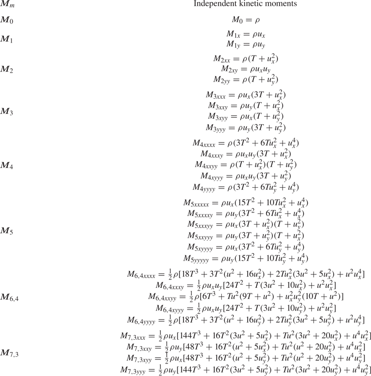
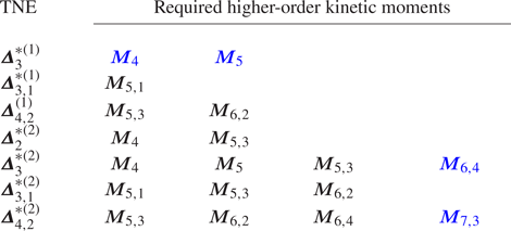
  $f_{i}^{(0)}$ should satisfy more higher-order non-equilibrium moments, as listed in table 1. Among them,
  $\boldsymbol {M}_{0}$,
  $\boldsymbol {M}_{1}$,
  $\boldsymbol {M}_{2}$,
  $\boldsymbol {M}_{3}$,
  $\boldsymbol {M}_{4}$,
  $\boldsymbol {M}_{5}$,
  $\boldsymbol {M}_{6,4}$ and
  $\boldsymbol {M}_{7,3}$ are independent (see Appendix C).
Table 1. Higher-order kinetic moment relations required for deriving the analytical expressions of TNE measures, where the blue terms are independent constraint relations.
Here, ‘satisfy’ means that the required kinetic moments of  $f_{i}^{(0)}$, originally in integral form, can be calculated in discrete summation form
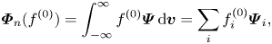 \begin{equation} \boldsymbol{\varPhi}_{n}(f^{(0)})=\int_{-\infty }^{\infty } f^{(0)}\boldsymbol{\varPsi }\, {\rm d} \boldsymbol{v}= \sum_{i}f_{i}^{(0)}\boldsymbol{\varPsi }_{i}, \end{equation}
with  $\boldsymbol {\varPsi }=[1,\boldsymbol {v},\boldsymbol {vv},\boldsymbol {vvv},\boldsymbol {vvvv}, \boldsymbol {vvvvv},\frac {1}{2}\boldsymbol {v}\boldsymbol {\cdot } \boldsymbol {vvvvv},\frac {1}{2}(\boldsymbol {v}\boldsymbol {\cdot } \boldsymbol {v})^{2}\boldsymbol {vvv}]^\textrm {T}$. Equation (2.31) can be rewritten in matrix form as
 \begin{equation} \boldsymbol{\varPhi }_{n}=\boldsymbol{\varPsi }\boldsymbol{\cdot} \boldsymbol{f}^{(0)}, \end{equation}
where  $\boldsymbol {\varPhi }_{n}=(\boldsymbol {M}_{0},\,\boldsymbol {M}_{1},\,\boldsymbol {M}_{2},\, \boldsymbol {M}_{3},\,\boldsymbol {M}_{4},\,\boldsymbol {M}_{5},\,\boldsymbol {M}_{6,4},\,\boldsymbol {M} _{7,3})^\textrm {T}\,=\,(M_{0},\,M_{1x},\,M_{1y},\ldots,$
  $M_{7,3yyy})^\textrm {T}$ is the set of moments of
  $f^{(0)}$. Also,
  $\boldsymbol {f} ^{(0)}=(f_{1}^{(0)},f_{2}^{(0)},\ldots,f_{30}^{(0)})^\textrm {T}$ and
  $\boldsymbol {\varPsi }=(\boldsymbol {C}_{1},\boldsymbol {C}_{2},\ldots,\boldsymbol {C}_{30})$ is a
  $30\times 30$ matrix bridging the DEDF and the kinetic moments with
  $\boldsymbol {C} _{i}=(1,v_{ix},v_{iy},\ldots,\frac {1}{2}v^{4}v_{ix}^{3},\frac {1}{2} v^{4}v_{ix}^{2}v_{iy},\frac {1}{2}v^{4}v_{ix}v_{iy}^{2},\frac {1}{2} v^{4}v_{iy}^{3})^\textrm {T}$. Naturally,
  $\boldsymbol {f}^{(0)}$ can be calculated as (Gan et al. Reference Gan, Xu, Zhang and Yang2013)
 \begin{equation} \boldsymbol{f}^{(0)}=\boldsymbol{\varPsi}{^{{-}1}} \boldsymbol{\cdot} \boldsymbol{\varPhi }_{n}, \end{equation}
where  $\boldsymbol {\varPsi }{^{-1}}$ is the inverse matrix of
  $\boldsymbol {\varPsi }$. Here, a two-dimensional DVM with
  $30$ discrete velocities, drawn in schematically figure 2, is used to discretize the velocity space and to ensure the existence of
  $\boldsymbol {\varPsi }{^{-1}}$:
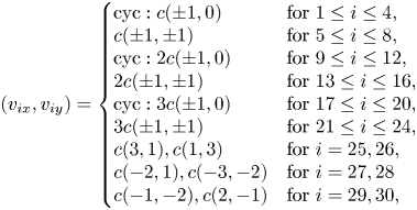 \begin{equation} (v_{ix},v_{iy})=\left\{ \begin{array}{@{}ll} \text{cyc}:c({\pm} 1,0) & \text{for}\ 1\leq i\leq 4, \\ c({\pm} 1,\pm 1) & \text{for}\ 5\leq i\leq 8, \\ \text{cyc}:2c({\pm} 1,0) & \text{for}\ 9\leq i\leq 12, \\ 2c({\pm} 1,\pm 1) & \text{for}\ 13\leq i\leq 16, \\ \text{cyc}:3c({\pm} 1,0) & \text{for}\ 17\leq i\leq 20, \\ 3c({\pm} 1,\pm 1) & \text{for}\ 21\leq i\leq 24, \\ c(3,1), c(1,3) & \text{for}\ i=25,26, \\ c({-}2,1), c({-}3,-2) & \text{for}\ i=27,28 \\ c({-}1,-2), c(2,-1) & \text{for}\ i=29,30, \end{array} \right. \end{equation}
where ‘cyc’ indicates cyclic permutation. The selection of  $\boldsymbol {v}_{25},\ldots,\boldsymbol {v}_{30}$ is highly flexible and thus guarantees the existence of
  $\boldsymbol {\varPsi }{^{-1}}$ and optimizes the stability of the model. Then the discrete coarse-grained evolution equation reads
 \begin{equation} \partial_{t}f_i+\boldsymbol{v}_i \boldsymbol{\cdot} \boldsymbol{\nabla}f_i={-}\frac{1}{\tau }\,[f_i-f^{(0)}_i]+I_i. \end{equation}
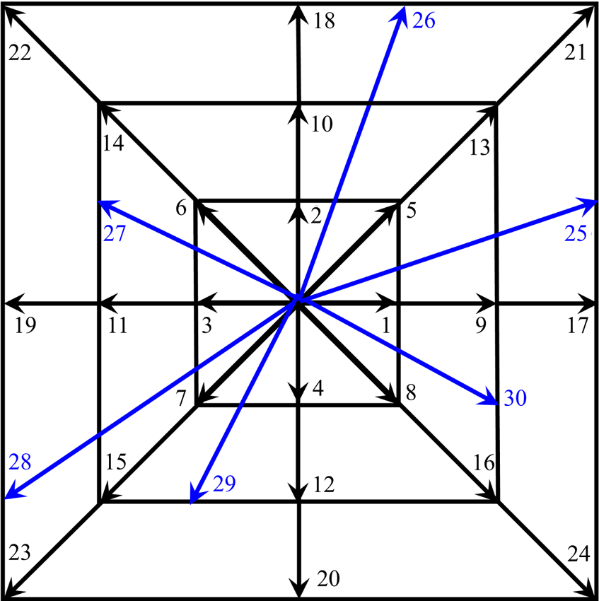
Figure 2. Schematic of the D2V30 discrete velocity model, where  $\boldsymbol {v} _{1},\boldsymbol {v}_{2},\ldots,\boldsymbol {v}_{24}$ are symmetric vectors, and
  $\boldsymbol { v}_{25},\boldsymbol {v}_{26},\ldots,\boldsymbol {v}_{30}$ are non-symmetric ones, designed to guarantee the existence of
  $\boldsymbol {\varPsi }{^{-1}}$.
It is necessary to point out the following.
(i) The most important step in DBM modelling and simulation is the calculation of
 $f_{i}^{(0)}$. The Maxwell distribution satisfies an infinite number of moment relations. Requiring $f_{i}^{(0)}$ to satisfy all the moment relations is impractical. Which moment relations are necessary depends on the kinetic properties to be studied, a choice that is typically dictated by the intensity of the non-equilibrium effects to be described.
(ii) The capability of describing non-equilibrium effects relies on the kinetic moment relations that the DBM retrieved correctly. Therefore, by satisfying different kinetic moments, we can systematically construct DBMs for TNE effects at various levels that correspond to different coarse-grained models and own different application ranges. For instance, besides the D2V30 DBM, we propose D2V13, D2V15 and D2V16 multiphase models, and examine their performances in the subsequent section. Here, the D2V13 (D2V15) model adopts the former 13 (15) discrete velocities of the D2V30 model. The D2V16 model indicates the one proposed in (Gan et al. Reference Gan, Xu, Zhang and Yang2013) for compressible flows with a flexible specific heat ratio. While considering only the translational degrees of freedom, the D2V16 model will degenerate into the D2V13 model. Independent kinetic moments retrieved by these models are exhibited in table 2.
(iii) For the same set of grids, the computational cost of the model is proportional to the number of discrete velocities. So, theoretically, the computational cost of the D2V30 model is twice that of the D2V15 model. Compared with the standard multiphase lattice Boltzmann model, such as the well-known Shan–Chen D2Q9 model (Wang et al. Reference Wang, Xu, Zhang and Li2009), the computational cost of the D2V30 model is about 4.4 times that of the D2Q9 model, greater than the ratio of the number of discrete velocities of the two DVMs,
$30/9$. This originates from the more concise external force term of the Shan–Chen model.(iv) The complexity of corresponding hydrodynamic equations increases sharply with the degree of TNE, whereas that of the DBM does not have a significant increase. We can formulate the DBM with the desired order of accuracy by incorporating more needed kinetic moments into
$\boldsymbol {\varPhi } _{n}$, and perform simulations without knowing the exact form of the hydrodynamic equations. For example, the D2V30 model satisfies 8 moment relations listed in table 2, and describes viscous stress and heat flux with third-order accuracy. If one wants to achieve fourth-order accuracy, then the physical model needs to further satisfy higher-order moment relations $\boldsymbol {M}_{6}$ and $\boldsymbol {M}_{7,5}$. Then the independent ones are $\boldsymbol {M}_{0}$, $\boldsymbol {M}_{1}$, $\boldsymbol { M}_{2}$, $\boldsymbol {M}_{3}$, $\boldsymbol {M}_{4}$, $\boldsymbol {M}_{5}$, $\boldsymbol {M} _{6}$ and $\boldsymbol {M}_{7,5}$. For a two-dimensional case, these moment relations have 34 independent components, so a D2V34 model is sufficient to discretize the phase space. Compared with the D2V30 model, the computational cost of the D2V34 model is increased by only $13.33\,\%$.(v) The Chapman–Enskog expansion acts as a bridge between the kinetic description given by the DBM and continuum mechanics non-conserved macroscopic dissipation and the conserved variables. Through it, we can determine directly and strictly the minimal physical requirements, and confirm the invariable moment sets
$\boldsymbol {\varPhi }_{n}$ for modelling a given non-equilibrium state. We also point out that from the perspective of perturbation theory, conducting Chapman–Enskog multi-scale analysis corresponds to imposing a disturbance on the equilibrium system. The convergence of Chapman–Enskog multi-scale expansion corresponds to the system returning to its equilibrium state. If the disturbance is too strong, such as due to the emergence of very steep gradients, leading to the divergence of the Taylor expansion of the distribution function, then the disturbance may trigger new structures or modes, and the Chapman–Enskog analysis fails. Fortunately, in the multiphase flow system, due to the existence of the interface with a certain width, the gradient of the macroscopic quantity is more gentle than that in the high-speed compressible single-phase system, especially in the low-speed multiphase flow with large surface tension.(vi) Strictly speaking, the discretization of continuous space inevitably brings non-physical symmetry breaking, and is a source of physical and numerical inaccuracies in the description of the system. Coarse-grained physical modelling is inherently a trade-off. The properties to be studied must be preserved during model simplification, beyond scope of the given study can be sacrificed. Of the many options available to meet the research needs of the current problem, the simplest or most economical is often the first choice. The moment matching approach, shown in (2.31), affords the minimal discrete velocity sets for solving
$\boldsymbol {\varPhi }_{n}$, because the number of discrete velocities just equals the number of independent kinetic moment relations. Therefore, physically, the DBM proposed in this way features the highest computational efficiency. These outstanding advantages make the DBM a particularly appealing methodology for investigating non-equilibrium flows. We can also build a more symmetrical DVM by increasing the number of discrete velocities. For example, we can construct a DVM through Hermite expansion (Shan et al. Reference Shan, Yuan and Chen2006; Zhang et al. Reference Zhang, Shan and Chen2006; Gan et al. Reference Gan, Xu, Zhang, Yu and Li2008; Li et al. Reference Li, Shi and Shan2019; Shi et al. Reference Shi, Wu and Shan2021) so that the DVM has better spatial symmetry at the cost of increasing the number of discrete velocities. In this paper, we have chosen the simplest form matching the relevant physical constraints for the problems at hand.(vii) For bulk flow far from the boundary, the DBM includes three main pillars, described in the Abstract. For near-wall flow, the mechanism for THNE may be greatly different from that for bulk flow, and consequently, a fourth pillar, construction of kinetic boundary conditions, is necessary. A DBM for slip flow is referred to in Zhang et al. (Reference Zhang, Xu, Chen, Lin and Wei2022b).
(viii) The present work belongs to the category of single-component miscible multiphase flow. There are several works on DBM modelling and simulation of multi-component miscible fluid flows (Lin et al. Reference Lin, Xu, Zhang and Li2016, Reference Lin, Luo, Fei and Succi2017, Reference Lin, Luo, Xu, Gan and Lai2021; Zhang et al. Reference Zhang, Xu, Zhang and Li2020). The extension of the present work to a multi-component immiscible fluid system is currently under consideration. For multi-component immiscible fluid flows, self-aggregation still occurs between different phases, and surface tension still exists between different components. The core of DBM modelling for immiscible multiphase flow is the incorporation of (a) intermolecular interaction in the same component, and (b) intermolecular interaction between different components.


Table 2. Discrete-velocity models and corresponding independent kinetic moments.
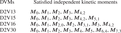
3. Numerical simulations and analysis
In this section, we first validate DBMs at various levels via three benchmarks related to the equilibrium properties in bulk regions. We then evaluate carefully the multi-scale predictive capability of the DBMs by investigating THNE features around the liquid–vapour interface. Finally, we study the effects of relaxation time and surface tension coefficient on thermal phase separation from the non-equilibrium aspects. In all simulations, we set  $a=2$ and
  $b=0.4$; then the critical density and temperature are
  $\rho ^{c}=1.30444$ and
  $T^{c}=1.88657$, respectively. To improve the numerical stability and accuracy, the windowed fast Fourier transform (FFT) scheme with
  $16$th-order precision (Gan et al. Reference Gan, Xu, Zhang, Li and Li2011, Reference Gan, Xu, Zhang, Zhang and Li2012b, Reference Gan, Xu, Zhang and Succi2015) is utilized to discretize the spatial derivatives, and the second-order Runge–Kutta scheme is used to calculate the temporal derivative. Notably, the periodic boundary condition is imposed inherently in the
  $x$ and
  $y$ directions because of the adoption of the FFT scheme. For a system with non-periodic boundary conditions, the FFT scheme can also be applied as long as the mirror operation is performed on the non-periodic boundary (Gan et al. Reference Gan, Xu, Zhang and Li2012a), at the cost of doubling the calculation amount. All the parameters used here are dimensionless. Please refer to Zhang et al. (Reference Zhang, Xu, Zhang, Gan, Chen and Succi2019) for recovery of the actual physical quantities from the numerical results.
3.1. Verification and validation
3.1.1. Liquid–vapour coexistence curve
Here, the liquid–vapour coexistence curve test is used to check if the newly constructed DBMs can reproduce the correct equilibrium thermodynamics of the Carnahan–Starling system. For the problem considered, the initial conditions are  $(\rho, T, u_{x}, u_{y})=(\rho _{l}, 1.82, 0.0, 0.0)$ if
  $N_{x}/4< x\leq 3N_{x}/4$, otherwise
  $(\rho, T, u_{x}, u_{y})=(\rho _{v}, 1.82, 0.0, 0.0)$, where
  $\rho _{l}=1.9643$ and
  $\rho _{v}=0.7569$ are the theoretical liquid and vapour coexisting densities at
  $T=1.82$. Parameters are
  $\tau =10^{-4}$,
  $K=1.5\times 10^{-4}$,
  $\Pr =0.01$,
  $N_{x}\times N_{y}=128\times 1$,
  $c=1.25$,
  ${\rm \Delta} t=3\times 10^{-5}$ and
  ${\rm \Delta} x={\rm \Delta} y=4\times 10^{-3}$ for the D2V13, D2V15 and D2V30 models. But in the D2V16 model, the minimum spatial step that stabilizes the simulation is
  ${\rm \Delta} x={\rm \Delta} y=5\times 10^{-3}$. The initial temperature drops by
  $0.01$ when a steady state has been reached, i.e.
  $|(u_{x}^{2}+u_{y}^{2})^{1/2}|_{max}<10^{-6}$. Figure 3 displays the phase diagrams calculated from the DBM simulations and Maxwell construction. In each panel, the two sets of results are in good agreement with each other. However, the maximum density ratio
  $R_{max }=\rho _{max }/\rho _{min}$ and the lowest reduced temperature
  $Tr_{min }=T_{min }/T^{C}$ that each model can undergo are quite different.
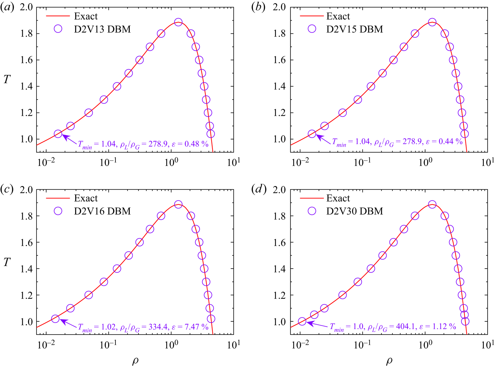
Figure 3. Comparisons of the coexisting densities predicted by various DBMs and Maxwell construction.
The more the moment relations maintained by the DBM, the larger the maximum density ratio and the lower the minimum reduced temperature that the model can attain. Specifically, in the D2V13 model,  $R_{max }=278.9$ with the maximum relative error in density
  $\epsilon =|\rho _{{DBM}}-\rho _{{Exact}}|/\rho _{{Exact}}=0.48\,\%$ in the vapour branch (
 $\epsilon _{{max}}=0.28\,\%$ for the D2V30 model under the same density ratio), whereas in the D2V30 model,
  $R_{max }$ can reach up to
  $404.1$ and
  $Tr_{min }$ reduces to
  $0.53$ with
  $\epsilon =1.12\,\%$ in the vapour branch.
There are several reasons that account for the fact that the incorporation of higher-order kinetic moments improves the density ratio that the model can sustain. First, physically, the incorporation of higher-order moment relations makes the DBM model more approximate to the continuous Boltzmann–BGK equation with an external force term; that is, the model is more physical. Second, the incorporation of higher-order moment relations makes the DBM more accurate in describing non-equilibrium effects, which greatly affects the computational accuracy and stability, as shown in figure 11. Third, the higher-order model is more capable of ensuring the positive entropy increase rate during the evolution process, with the entropy growth rate defined as (Zhang et al. Reference Zhang, Xu, Zhang, Gan, Chen and Succi2019)  ${\textrm {d} S}/{\textrm {d} t}=\int (\boldsymbol {\varDelta }_{3,1}^{\ast }\boldsymbol {\cdot } \boldsymbol {\nabla }({1}/{T})- ({1}/{T})\boldsymbol {\varDelta }_{2}^{\ast }: \boldsymbol {\nabla }\boldsymbol {u})\, \textrm {d} \boldsymbol {r}$. Fourth, the incorporation of higher-order moment relations is equivalent to adopting more discrete velocities to discretize the phase space. As the number of discrete velocities increases, the fluctuations of distribution function
  $\delta f$ and the spatial gradient of distribution function
  $\boldsymbol {\nabla }f$ decrease, which makes the higher-order model more stable. Lots of numerical examples suggest that the stability improvement of the higher-order model compared to lower-order ones is effective not only for static (or quasi-static) tests, but also for dynamic cases.
3.1.2. Spurious velocity
Figure 4 illustrates the time evolutions of the maximum velocity  $u_{max }$ for an initially non-equilibrium planar interface, obtained from various DBM simulations performed using the procedure and parameters exhibited in figure 3, except that the initial temperature is suddenly quenched from
  $1.45$ to
  $1.10$, and the relaxation time is
  $\tau =2\times 10^{-4}$. The spurious velocity, located mainly around the liquid–vapour interface, refers to the residual velocity, which cannot be further reduced after a long period of evolution (Wagner Reference Wagner2003). Specifically, for the D2V30 model, spurious velocity refers to the remaining current when
  $t>120$ in figure 4. The decay before
  $t<120$ is a physical process decided by the initial condition.
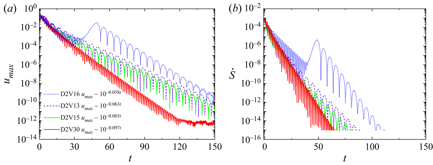
Figure 4. (a) Time evolutions of the maximum velocity  $u_{{max}}$ calculated from various DBMs. (b) Time evolutions of the entropy increase rate.
Discarding the early-time transient regime and the very-late-time regime, where  $u_{max }$ stays almost unchanged, we find that
  $u_{max}$ decreases with time
  $t$ approximately as
  $u_{max }\sim 10^{-\gamma t}$. But the exponent of the D2V30 model (
 $\gamma \simeq 0.1$) is considerably larger than that of other models (
 $\gamma \sim 0.061\pm 0.003$). When
  $t>120.0$,
  $u_{max }$ decays to a negligible value
  $10^{-12}$ in the D2V30 simulation under the combined effects of NOMF and NOEF. Figure 4(b) shows time evolutions of entropy increase rate for the decaying process. When the system temperature is fixed, the entropy increase rate reduces to
  ${\textrm {d} S}/{\textrm {d} t}=-\int ({1}/{T})\boldsymbol {\varDelta }_{2}^{\ast }: \boldsymbol {\nabla }\boldsymbol {u}\, \textrm {d} \boldsymbol {r}$. The slope of the entropy increase rate reflects the speed at which the system tends towards equilibrium, which is qualitatively consistent with figure 4(a). The larger the slope of the entropy increase rate, the faster the decay in
  $u_{{max}}$. Compared with lower-order models, a faster decay in
  $u_{{max}}$ obtained from the D2V30 model is due to a more accurate viscous stress that the model recovers. These findings suggest that the retrieval of higher-order kinetic moments in physical modelling makes the DBM more powerful in inhibiting spurious currents.
3.1.3. Conservativeness of the new model
To examine the conservativeness of the new model, we monitor variations in  $\rho$,
  $\rho \boldsymbol {u}$ and
  $e_{T}$ in a thermal phase transition process in figure 5. The initial conditions are
  $(\rho, T, u_{x}, u_{y})=(1.5+\varDelta, 1.0, 0.0, 0.0)$, where
  $\varDelta$ is a random noise of the amplitude
  $0.001$ acting as heterogeneous nuclei and accelerating the kinetic process. The remaining parameters are
  $N_{x}=N_{y}=128$,
  $\tau =10^{-3}$,
  $K=5\times 10^{-5}$ and
  $\Pr =0.1$. Even when the system is quenched instantaneously to a completely unstable state, the two models maintain
  ${\rm \Delta} \rho$ and
  ${\rm \Delta} (\rho \boldsymbol {u})$ to machine accuracy. Meanwhile, it is found that
  $\delta (\rho u)$ is two orders of magnitude lower than
  $\delta (\rho )$. This is because: (a)
  $\delta (\rho u)=u\,\delta \rho +\rho \,\delta u$; (b) different from the isothermal phase separation process, the release of latent heat causes the changing of local temperature. The freedom in temperature results in a more detailed and stricter local mechanical and thermodynamic equilibrium, consequently hampering the full development of velocity, especially for the case with large viscosity. The mean velocity
  $u_{{mean}}$ is approximately of the order of
  $10^{-2}$ throughout the simulations that we considered. So
  $u\delta \rho \sim 10^{-15}$. (c) Furthermore, it is reasonable that variations in
  $\rho (t)$ and
  $\rho u(t)$ are proportional to their fluctuations,
  $\delta \rho \propto (\rho _{max }-\rho _{min })\sim o(1)$ and
  $\delta u\propto (u_{max }-u_{min })\sim o(10^{-2})$, so
  $\delta u$ is two orders of magnitude lower than
  $\delta \rho$. Then
  $\rho \,\delta u\sim 10^{-15}$.
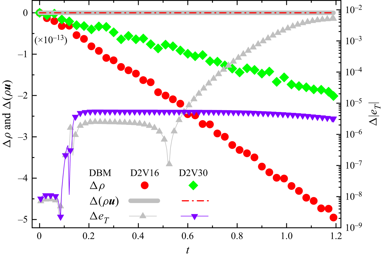
Figure 5. Variations in  $\rho$,
  $\rho \boldsymbol {u}$ and
  $e_{T}$ in a thermal phase separation process obtained from D2V16 and D2V30 DBMs.
In our simulations, the average energy density  $e_{T}=\rho T-a\rho ^{2}+K\,|\boldsymbol {\nabla }\rho |^{2}/2+\rho u^{2}/2=$
  $-3.000015$. Different from
  ${\rm \Delta} \rho$ and
  ${\rm \Delta} (\rho \boldsymbol {u})$,
  ${\rm \Delta} e_{T}(t)$ oscillates and grows persistently during the whole procedure mimicked by the D2V16 model. Two reasons account for the oscillation and growth in
  ${\rm \Delta} e_{T}(t)$. First, the appearance of numerous liquid–vapour interfaces in the spinodal decomposition stage induces macroscopic quantity gradients and accumulated spatial discretization errors. Second, the resulting macroscopic quantity gradients serve as sources of HNE and TNE that may threaten the validity of the lower-order DBM. The maximum deviation of
  $e_{T}(t)$ is
  $0.01$ for the D2V16 model, while it is
  $O(10^{-6})$ for the D2V30 model, demonstrating that the D2V30 model is more effective in maintaining energy conservation and more capable of handling typical non-equilibrium processes. These variations are indicators of model accuracy that significantly affect the phase morphology, flow field distribution and stability of simulation.
The results for two-dimensional lattices with 13, 15, 16 and 30 velocities indicate that increasing the order of approximation of the lattice Boltzmann equation enhances performance in maintaining thermodynamic consistency, energy conservation, and inhibiting spurious currents.
3.2. Multi-scale model and trans-scale ability
In the DBM modelling, there exist two sets of macroscopic variables, the conservative set ( $\rho$,
  $\rho \boldsymbol {u}$,
  $e_{T}$) and the non-conservative counterpart (
 $\boldsymbol {\varDelta }_{m,n}$ and
  $\boldsymbol {\varDelta }_{m,n}^{\ast }$,
  $m-n \geq 2$), which vary in diverse time and length scales. Compared with the slowly varying conservative variables, the THNE quantities are quickly varying non-conservative ones, with extremely short relaxation times of the order of
  $10^{-10}$ s (Myong Reference Myong1999). In this subsection, we evaluate carefully the multi-scale predictive capability of the DBMs for describing THNE features. Specifically, we determine whether or not the DBM can correctly capture the fast-changing THNE characteristics around an evolving liquid–vapour interface. Indeed, understanding precisely the fine structure and the specific status of non-equilibrium state between two phases at coexistence is of central importance in a variety of fields, because these non-equilibrium characteristics determine the transport efficiency of mass and energy across an interface, as well as the growth dynamics and morphological behaviours.
To date, significant progress has been made by pioneers in the non-equilibrium effects of multiphase flows. Frezzotti et al. comprehensively studied the rich array of non-equilibrium effects of multiphase flows through solving numerically the Enskog–Vlasov equation by direct simulation Monte Carlo (Enskog-Vlasov DSMC) and through the molecular dynamics (MD) method (Frezzotti, Gibelli & Lorenzani Reference Frezzotti, Gibelli and Lorenzani2005; Frezzotti Reference Frezzotti2011; Frezzotti & Rossi Reference Frezzotti and Rossi2012; Frezzotti et al. Reference Frezzotti, Gibelli, Lockerby and Sprittles2018; Frezzotti, Barbante & Gibelli Reference Frezzotti, Barbante and Gibelli2019), including the non-equilibrium structure of the liquid–vapour interface, velocity slip at the liquid–vapour boundary, non-equilibrium evaporation, and non-equilibrium stress. In addition to microscopic MD and mesoscopic DSMC, recently, the extended macroscopic moment method, in particular the regularized moment method (Struchtrup & Torrilhon Reference Struchtrup and Torrilhon2003; Struchtrup Reference Struchtrup2005; Chen et al. Reference Chen, Zhao, Jiang and Liui2016; Torrilhon Reference Torrilhon2016), derived as approximations of the Boltzmann equation by means of the order-of-magnitude method, has been developed rapidly and extended to the field of multiphase flows (Struchtrup et al. Reference Struchtrup, Beckmann, Rana and Frezzotti2017; Struchtrup & Frezzotti Reference Struchtrup and Frezzotti2022) by Struchtrup et al. In Struchtrup et al. (Reference Struchtrup, Beckmann, Rana and Frezzotti2017), the macroscopic evaporation boundary conditions for regularized 13 (R13) moment equations have been derived from microscopic interface conditions of the Boltzmann equation, which extends the application range of the R13 equation to multiphase flows in the transition regime. More recently, in Struchtrup & Frezzotti (Reference Struchtrup and Frezzotti2022), a set of 26 moment equations for the Enskog–Vlasov equation has been derived by using the Grad moment method, which provides a computationally efficient and functionally unified approach for ideal and non-ideal fluid flows far from equilibrium. Besides, the coupled constitutive relations theory was developed to capture the remarkable rarefaction effects at small scales in the liquid–vapour phase transition processes (Rana et al. Reference Rana, Saini, Chakraborty, Lockerby and Sprittles2021). Meanwhile, the rarefaction effects in a head-on collision of two identical droplets are investigated via various lattice Boltzmann models with different degrees of precision (Chen et al. Reference Chen, Wu, Wang and Chen2022b). It is found that the rarefaction effects enhance the conversion from free energy to kinetic energy, and accelerate droplet coalescence. Parsa et al. presented an original and fundamental molecular dynamics lattice gas (MDLG) approach connecting lattice Boltzmann methods to physical reality (Parsa & Wagner Reference Parsa and Wagner2017, Reference Parsa and Wagner2020; Czelusniak et al. Reference Czelusniak, Mapelli, Guzella, Cabezas-Gómez and Wagner2020; Pachalieva & Wagner Reference Pachalieva and Wagner2021; Parsa, Kim & Wagner Reference Parsa, Kim and Wagner2021). The key implementation of MDLG is an embedded coarse-graining procedure, i.e. mapping an MD simulation onto a lattice Boltzmann framework. It permits us to study any system that can be simulated with MD, including the non-ideal system with significant non-equilibrium fluctuations (Parsa & Wagner Reference Parsa and Wagner2020), since the collision operator is informed by an underlying MD simulation. This approach can be considered as an optimal LBM or a more realistic coarse-grained fluctuating method. We stress that these microscopic (MD), mesoscopic (DSMC, LBM and DBM proposed here) and macroscopic (high-order moment method, extended hydrodynamics or generalized hydrodynamics models) models/methods, with different starting points and different emphases, have their own strengths and insights, and complement each other, but cannot replace each other. In addition, the developments of these methods have stages.
Although extensive experimental and theoretical studies have been designed and developed in the past decades to address this issue (Weeks Reference Weeks1977; Evans Reference Evans1979; Bedeaux Reference Bedeaux1986; Onuki Reference Onuki2002; Aarts, Schmidt & Lekkerkerker Reference Aarts, Schmidt and Lekkerkerker2004; Lang & Leiderer Reference Lang and Leiderer2006; Bu, Kim & Vaknin Reference Bu, Kim and Vaknin2014; Jaensson & Vermant Reference Jaensson and Vermant2018), the early stage of the liquid–vapour transition, i.e. the spinodal decomposition stage, where non-equilibrium effects are much more pronounced than the latter domain growth stage, still needs further investigations from the viewpoint of non-equilibrium thermodynamics. Early studies tend to focus on conserved quantities and slow variables, because these characteristics are relatively stable and easy to grasp (Osborn et al. Reference Osborn, Orlandini, Swift, Yeomans and Banavar1995; Gonnella et al. Reference Gonnella, Orlandini and Yeomans1997, Reference Gonnella, Lamura and Sofonea2007, Reference Gonnella, Lamura, Piscitelli and Tiribocchi2010; Succi Reference Succi2001; Xu et al. Reference Xu, Gonnella and Lamura2003; Sofonea et al. Reference Sofonea, Lamura, Gonnella and Cristea2004; Onuki Reference Onuki2007, Reference Onuki2002; Gan et al. Reference Gan, Xu, Zhang, Li and Li2011, Reference Gan, Xu, Zhang, Zhang and Li2012b; Coclite et al. Reference Coclite, Gonnella and Lamura2014). The study of these conserved quantities and slow variables provides a basis for the study of fast-changing behaviour that is particularly relevant to the early stage of spinodal decomposition, a process still far from being completely understood.
The reason is that these fast-varying and complex THNE quantities springing up in the spinodal decomposition stage are difficult to measure and analyse. Moreover, related experiments are costly and time-consuming. Theoretical analysis is usually limited to cases with numerous simplifying assumptions and generalizations, such as the local equilibrium assumption, given small deviations from the equilibrium state and linear relationship between fluxes and forces. How to overcome these limitations is a core problem in physical modelling (Gurtin & Voorhees Reference Gurtin and Voorhees1996; Vilar & Rubi Reference Vilar and Rubi2001; Schweizer, Öttinger & Savin Reference Schweizer, Öttinger and Savin2016; Rana et al. Reference Rana, Saini, Chakraborty, Lockerby and Sprittles2021).
The definition of any non-equilibrium strength depends on the perspective of the study. Complex systems need to be investigated from multiple perspectives. If we look at the system from  $N$ angles, then there are
  $N$ kinds of non-equilibrium strengths. Therefore, if the
  $N$ kinds of non-equilibrium strengths are taken as components to introduce a non-equilibrium strength vector, then it should be more accurate and specific. Below, we use the four-component vector
  $\boldsymbol {S}_{{THNE}} = (\boldsymbol {\varDelta }_{2}, \boldsymbol {\varDelta }_{3,1}, \boldsymbol {\varDelta }_{3}, \boldsymbol {\varDelta }_{4,2} )$, whose analytical expressions have been derived, to describe roughly the strength of non-equilibrium.
3.2.1. Weak THNE case
According to the analytical formulas listed in Appendix B and § 2.1, four explicit factors control the intensities and structures of THNE manifestations, i.e. the relaxation time  $\tau$, the fluid velocity
  $\boldsymbol {u}$, the gradient force, and the interparticle force caused by gradients of macroscopic quantities. The latter are affected implicitly by the initial state and the duration of evolution, for example, the initial density distribution, the quenching temperature, the surface tension coefficient, and the Prandtl number. Therefore, by adjusting these aspects, we can design scenarios with weak, moderate and strong THNE strengths.
First, we investigate the weak THNE case. The initial state is the equilibrium density profile  $\rho _{{initial}}(x)$ at
  $T=1.74$, as shown in figure 6(c). The parameters are
  $K=2.7\times 10^{-5}$,
  ${\rm \Delta} t=2\times 10^{-5}$ and
  ${\rm \Delta} x={\rm \Delta} y=5\times 10^{-3}$; others are consistent with those in figure 3. When simulation starts, the system is suddenly quenched to
  $T=1.0$. The profiles of hydrodynamic quantities, including the chemical potential (Wagner Reference Wagner2006; Wen et al. Reference Wen, Zhou, He, Zhang and Fang2017, Reference Wen, Zhao, Qiu, Ye and Shan2020)
  $\mu ^{{CS}}=RT[({3-b\rho /4 })/{(1-b\rho /4 )^{3}}+\ln \rho +1]-2a\rho -K\,\nabla ^{2}\rho$, calculated from the D2V30 model at representative instants, are shown in figure 6, where
  $\phi _{n}$ represents the macroscopic quantity after
  $n$ iterations. The following results have been obtained. (i) The instantaneous decrease in temperature results in the emergence of steep gradients in both pressure
  $P^{{CS}}$ and chemical potential
  $\mu ^{{CS}}$ near the liquid–vapour interfaces (see figure 6a). (ii) The pressure and chemical potential gradients drive the vapour phase across the interface towards the liquid phase (see figures 6b,c), contributing to the decrease (increase) in vapour (liquid) density, and the appearance of remarkable velocity around the interface. After
  $20$ iterations, the maximum velocity along the
  $x$ direction,
  $u_{x-max}$, is approximately
  $0.04$, but it exceeds
  $0.80$ after
  $500$ iterations. (iii) With the development of phase separation, latent heat is released locally to and absorbed by the surrounding liquid and vapour phases, respectively. These processes lead to violent changes in temperature and local mechanical imbalance. The maximum temperature difference between the two phases
  ${\rm \Delta} T_{max }$ is negligible at the very beginning of the procedure, but reaches
  $0.6T_{{ initial}}$ at
  $t=0.01$ (
 $500$ iterations), which is the largest difference from an isothermal case at a fixed temperature.
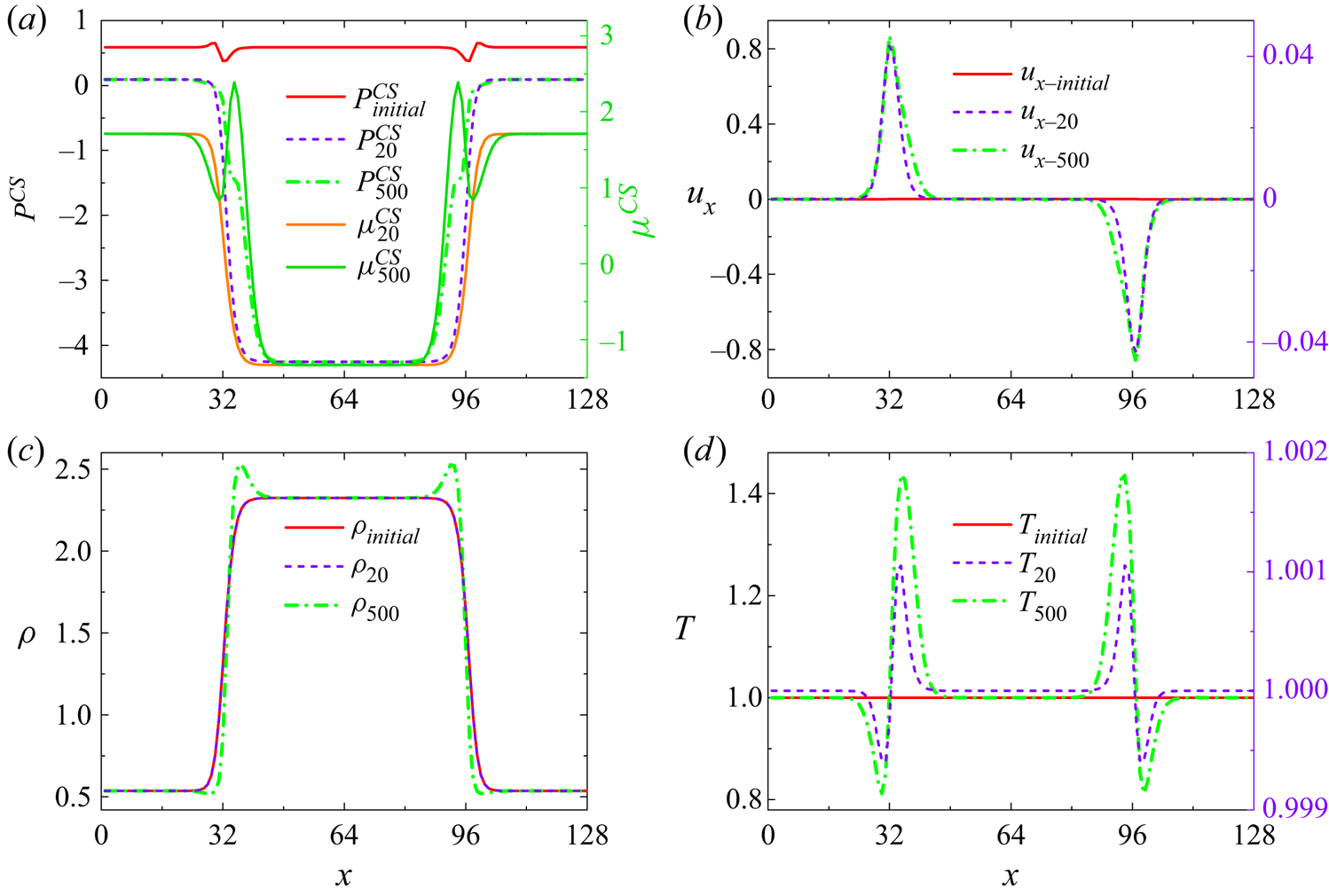
Figure 6. Profiles of hydrodynamic quantities calculated from the D2V30 model at three representative instants:  $0$,
$0$,  $20$ and
  $500$ iterations.
Figure 7 portrays the specific THNE manifestations  $\varDelta _{2xx}$,
  $\varDelta _{3,1x}$,
  $\varDelta _{3xxx}$, and
  $\varDelta _{4,2xx}$ for figure 6 at
  $t=4\times 10^{-4}$ (
 $20$ iterations), where the D2V13 model at the NS level (left column), the D2V15 model at the NS level (middle column), and the D2V30 model beyond the third-order super-Burnett level (right column) have been adopted. For the convenience of comparisons, analytical solutions with the first- and second-order accuracies are plotted by solid lines. Figure 7 shows the following general characteristics when the system deviates from thermo-hydrodynamic equilibrium. (i) THNE effects concentrate primarily in the interfacial regions, where the interparticle force and gradient force dominate, and disappear in the same manner as the gradients of macroscopic quantities vanish in the liquid and vapour bulk phases. (ii) Owing to the limited action time of the gradient force and interparticle force, THNE effects are not fully developed until this moment. (iii) The first-order THNE,
  $\boldsymbol {\varDelta }_{m,n}^{(1)}\propto \tau$, is always larger than the second-order THNE,
  $\boldsymbol {\varDelta }_{m,n}^{(2)}\propto \tau ^{2}$, demonstrating that
  $\boldsymbol {\varDelta }_{m,n}^{(1)}$ is the principal part of
  $\boldsymbol {\varDelta }_{m,n}$ and, to some extent, the effectiveness of the lower-order coarse-grained model. (iv) It is interesting to find that
  $|\boldsymbol {\varDelta }_{m,n}^{(1)}+\boldsymbol {\varDelta }_{m,n}^{(2)}|$ is not larger than
  $|\boldsymbol {\varDelta }_{m,n}^{(1)}|$, i.e. the second-order THNE invariably acts as negative feedback on the first-order one, and weakens the total THNE intensity.
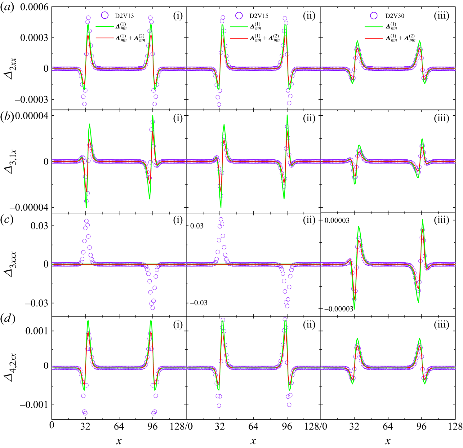
Figure 7. Weak case: THNE manifestations calculated from DBMs at various levels and theoretical analysis. Here,  $t=4\times 10^{-4}$ (
 $20$ iterations) and
  $\tau =10^{-4}$.
Beyond the aforementioned commonalities, the following distinctive performances among various models should be examined thoroughly. It is clear that even with such a feeble THNE, the simulation results of the D2V13 and D2V15 models do not match well, with either the first-order or the second-order theoretical solutions. More explicitly, the two lower-order models overestimate the THNE level tremendously, especially on the vapour side and for the  $xxx$ component of
  $\boldsymbol {\varDelta }_{3}$. The discrepancies possess peak values approximately at the locations where the gradient of the most associated physical quantity reaches its local maximum (minimum).
Two key factors are responsible for the failure of the lower-order DBM in capturing THNE accurately. On the one hand, to fully describe a given non-equilibrium quantity  $\boldsymbol {\varDelta }_{m,n}^{(\kern0.06em j)}$, the number of the required kinetic moments retrieved exactly by the discrete equilibrium distribution function
  $\,f_{i}^{(0)}$ increases with increasing
  $m$, i.e. the rank of
  $\boldsymbol {\varDelta }_{m,n}$. As shown in table 1, in the formulation of
  $\boldsymbol {\varDelta }_{3,1}^{(1)}$,
  $f_{i}^{(0)}$ should satisfy the moment
  $\boldsymbol {M}_{5,1}$; when deriving
  $\boldsymbol {\varDelta }_{4,2}^{(1)}$,
  $f_{i}^{(0)}$ should satisfy higher-order moments
  $\boldsymbol {M}_{5,3}$ and
  $\boldsymbol {M}_{6,2}$. On the other hand, additional moment constraints on
  $f_{i}^{(0)}$ need to be selected and guaranteed with increasing
  $j$, i.e. the order of accuracy of
  $\boldsymbol {\varDelta }_{m,n}$. Concretely, a first-order accuracy in the description of
  $\boldsymbol {\varDelta }_{3}^{{}}$ can be achieved by maintaining
  $\boldsymbol {M}_{4}$ and
  $\boldsymbol {M}_{5}$; while realizing a second-order accuracy in the description of
  $\boldsymbol {\varDelta }_{3}$,
  $f_{i}^{(0)}$ should further retain the additional thermodynamic one,
  $\boldsymbol { M}_{6,4}$ (
 $\boldsymbol {M}_{5,3}$ in table 1 is not independent of
  $\boldsymbol {M}_{5}$). Table 2 manifests that both the D2V13 and D2V15 models cannot hold these necessary constraint relationships, even just for the first-order accurate descriptions of
  $\boldsymbol {\varDelta }_{3,1}^{(1)}$ and
  $\boldsymbol {\varDelta }_{4,2}^{(1)}$. Among these THNE quantities, the correct description of
  $\boldsymbol {\varDelta }_{3}$ and
  $\boldsymbol {\varDelta }_{4,2}$ requires the retrieval of the highest-order moment relations. Thus, as expected, the worst simulation results appear in figures 7(c.i), (c.ii), (d.i) and (d.ii), provided by the two lower-order models.
Compared with the D2V13 model, the supplemental moment  $\boldsymbol {M}_{5,1}$, which is necessary for the formulation of
  $\boldsymbol {\varDelta }_{3,1}^{(1)}$ and maintained by the D2V15 model, plays a fairly negligible role in improving the numerical precision of
  $\varDelta _{3,1x}$, because the second-order non-equilibrium effects
  $\boldsymbol {\varDelta }_{m,n}^{(2)}$ cannot be neglected in contrast to the first-order
  $\boldsymbol {\varDelta }_{m,n}^{(1)}$ during the early stage of spinodal decomposition. Under this condition, considering the first-order THNE effects only is not recommended. Indeed, at the beginning of the phase separation, the gradients of temperature and velocity approximately equal zero. As a result,
  $\varDelta _{2xx}^{(1)}\simeq 0$, and
  $\varDelta _{2xx}^{(2)}$ can be simplified to
  $({T^{2}}/{\rho }) (\partial _{x}\rho )^{2}-T^{2}({\partial ^{2}\rho }/{\partial x}^{2})-\rho T^{2}\partial _{x}B_{x}$. These higher-order terms in
  $\varDelta _{2xx}^{(2)}$ do not appear in classical hydrodynamics, but are essential for modelling a system far from equilibrium (Struchtrup Reference Struchtrup2005; Struchtrup & Frezzotti Reference Struchtrup and Frezzotti2022). Other non-equilibrium measures can be analysed similarly. That is, interparticle force and density gradient force first trigger the second-order THNE, and afterwards, stimulate the first-order THNE through enlarging velocity and temperature gradients. To evaluate under which circumstances the higher-order THNE should be taken into account, a characteristic dimensionless parameter, called the relative THNE strength
  $R_{{THNE}}=|\boldsymbol {\varDelta }_{m,n}^{(j+1)}/\boldsymbol { \varDelta }_{m,n}^{(\kern0.06em j)}|$, may be introduced for the estimation of the relative importance of the
  $(j+1)$th-order THNE effects to the
  $j$th-order ones. The
  $R_{{THNE}}$ for
  $\varDelta _{2xx}$,
  $\varDelta _{3,1x}$,
  $\varDelta _{3xxx}$ and
  $\varDelta _{4,2xx}$ at the positions where these non-equilibrium measures take extreme values, are
  $0.250$,
  $0.349$,
  $0.212$ and
  $0.252$, respectively. At earlier times, such as after
  $15$ iterations,
  $R_{{THNE}}$ is as high as
  $0.50$. Therefore, higher-order DBMs with at least second-order accuracy for
  $\boldsymbol {\varDelta }_{m,n}$ are undoubtedly needed, even for cases with faint non-equilibrium effects. Tables 1 and 2 indicate that the D2V30 model satisfies all the needed kinetic moment relations. Consequently, the D2V30 results are consistent with the theoretical analysis at the second order of accuracy. In particular, the remarkable deviations in figures 7(c.i) and (c.ii) disappear in figure 7(c.iii).
3.2.2. Moderate THNE case
As time evolves, the degree of phase separation becomes pronounced, with extended phase-separating regions and prominent gradients of macroscopic quantities (see dash-dot lines in figure 6). The non-equilibrium manifestations at the same instant, exhibited in figure 8, indicate that the system enters into the moderate THNE stage. Compared with figure 7, the most distinctive difference in figure 8 is the enormous growth in  $\boldsymbol {\varDelta }_{m,n}$, approximately
  $10\unicode{x2013} 1000$ times larger than in the weak case. For each kind of THNE quantity, the first-order analytical solution (denoted by green dots) overlaps with the second-order one (denoted by red solid lines), illustrating that
  $\boldsymbol {\varDelta }_{m,n}^{(2)}$ is negligible compared with
  $\boldsymbol {\varDelta }_{m,n}^{(1)}$. Correspondingly, the relative THNE strengths
  $R_{{THNE}}$ for
  $\varDelta _{2xx}$,
  $\varDelta _{3,1x}$,
  $\varDelta _{3xxx}$ and
  $\varDelta _{4,2xx}$ are as small as
  $0.006$,
  $0.002$,
  $0.018$ and
  $0.016$, respectively. For
  $\varDelta _{2xx}$, good agreements between simulations and theoretical solutions are depicted in figures 8(a.i) and (a.ii). This is understandable because either of the D2V13 and D2V15 models is a sufficient description of
  $\varDelta _{2xx}^{(1)}$. Nevertheless, for
  $\varDelta _{3,1x}$, owing to the lack of indispensable kinetic moment
  $\boldsymbol {M}_{5,1}$ in the D2V13 model, distinct discrepancies are found in figure 8(b.i), but are absent in figure 8(b.ii), obtained from the D2V15 model that meets the constraint of
  $\boldsymbol {M}_{5,1}$. Similarly, for
  $\varDelta _{3xxx}$ and
  $\varDelta _{4,2xx}$, the D2V13 and D2V15 results mismatch the theoretical profiles, because of the deficiencies in the necessary high-order moments
  $\boldsymbol {M}_{4}$,
  $\boldsymbol {M}_{5}$ and
  $\boldsymbol {M}_{6,2}$. By contrast, as shown in the third column of figure 8, the D2V30 results coincide excellently with the theoretical results, regardless of the relative non-equilibrium intensity. We also stress that if we focus only on the hydrodynamic quantities and constitutive relations (related to
  $\boldsymbol {\varDelta }_{2}$ and
  $\boldsymbol {\varDelta }_{3,1}$), but not the evolution of the constitutive relations (related to
  $\boldsymbol {\varDelta }_{3}$ and
  $\boldsymbol {\varDelta }_{4,2}$), then the D2V15 model is reliable and acceptable when
  $R_{{THNE}}$ is small enough.
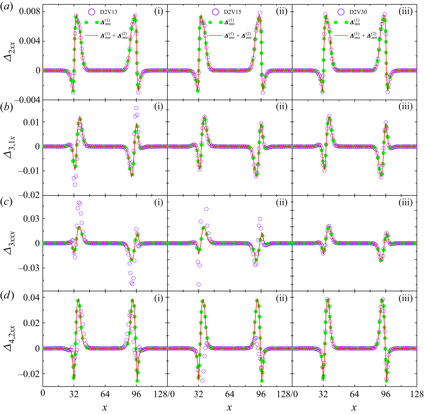
Figure 8. Moderate case: non-equilibrium manifestations calculated from DBMs at various levels and theoretical analysis. Here,  $t=0.01$ (
 $500$ iterations) and
  $\tau =10^{-4}$.
3.2.3. Strong THNE case
To further examine the multi-scale ability of the models, we increase the strength of THNE measures by straightforwardly increasing the relaxation time  $\tau$ in figure 9. In addition, another way to control the THNE strength is by adjusting the quenching depth
  $T/T_C$, which indirectly affects the non-equilibrium intensity by changing the gradients of hydrodynamic quantities. With the increasing of THNE intensity, deviations between lower-order DBM simulations and theoretical solutions become extraordinarily conspicuous (see the first and second columns of figure 9). The relative THNE strengths
  $R_{{THNE}}$ for
  $\varDelta _{2xx}$,
  $\varDelta _{3,1x}$,
  $\varDelta _{3xxx}$ and
  $\varDelta _{4,2yy}$ rapidly reach up to
  $0.213$,
  $0.248$,
  $0.169$ and
  $0.239$, respectively, manifesting the importance of the second-order THNE and the urgent need for a higher-order DBM. The D2V30 model meets the minimum physical requirements in describing accurately the concerned THNE quantities. Therefore, the reasonable agreements between D2V30 simulations and corresponding theoretical solutions in the weak, moderate and strong THNE cases demonstrate comprehensively that the D2V30 DBM is indeed a multi-scale model and possesses better trans-scale ability than the D2V13 and D2V15 models.
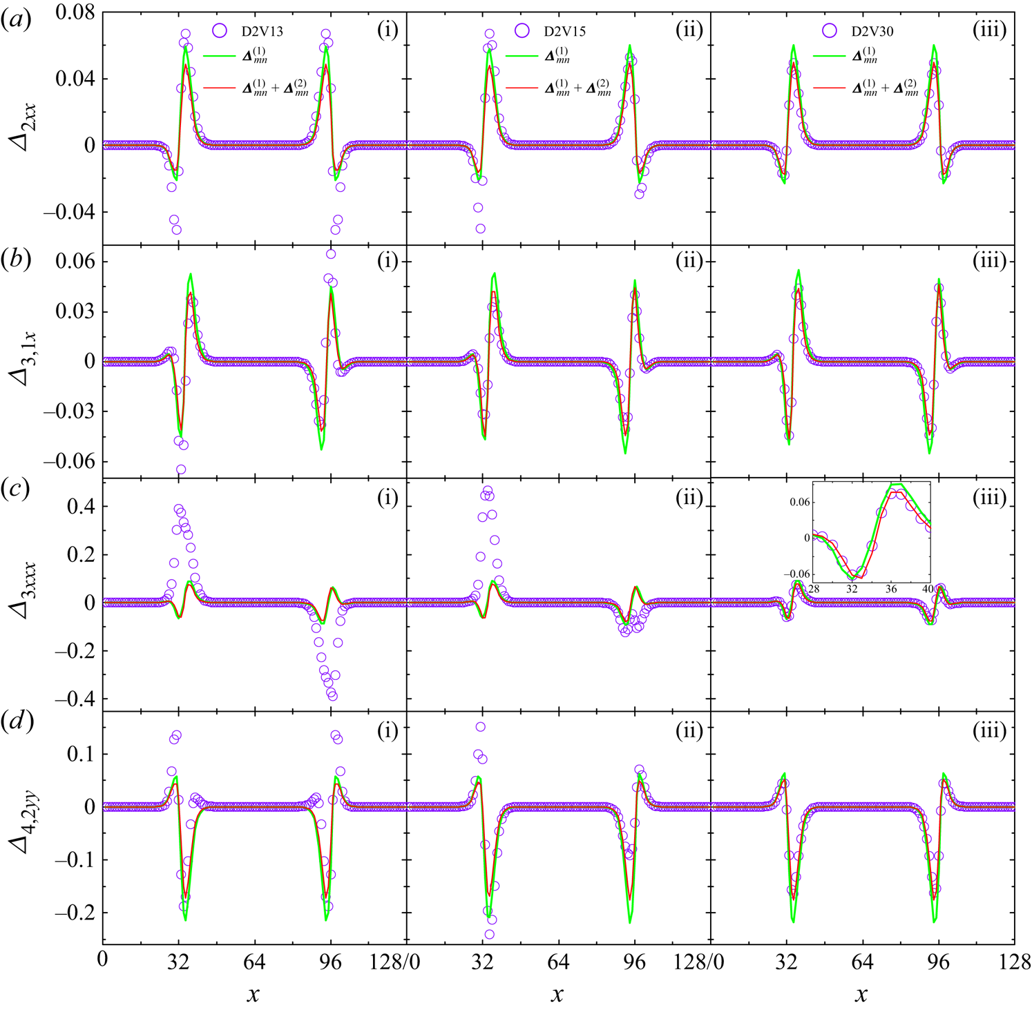
Figure 9. Strong case: non-equilibrium manifestations calculated from DBMs at various levels and theoretical analysis. Here,  $t=0.006$ (
 $300$ iterations) and
  $\tau =10^{-3}$.
To assess the application range of the DBM more completely, we resort to the Knudsen number, a dimensionless parameter generally used to characterize non-equilibrium or rarefaction degree of flows, and classify various flow regimes. The Knudsen number  $Kn=\lambda /L$ is defined as the ratio of the mean free path
  $\lambda =c_{s}\tau$ to a characteristic length that we focus on,
  $L=\varTheta /|\boldsymbol {\nabla }\varTheta |$, where
  $c_{s}$ is the local speed of sound, and
  $\varTheta$ is a physical quantity. The maximum
  $Kn_{max }$ values calculated by density for cases with weak, moderate and strong THNE effects are
  $0.008$,
  $0.015$ and
  $0.141$, respectively, all beyond the application scope of NS equations. Evidently, the applicable range of the D2V30 model has been extended into the early transition regime.
3.3. Effects of relaxation time on TNE
In this subsection, we investigate the multi-scale limit of the D2V30 model through exploring whether the model can correctly reproduce higher-order constitutive relations for multiphase flows over a wide range of relaxation times and Knudsen numbers. Essentially, the accurate description of constitutive relations is of fundamental importance to the simulation of highly non-equilibrium multiphase flows (Struchtrup Reference Struchtrup2005). It is the constitutive relations that determine directly the multi-scale ability and accuracy of a model. For this purpose, in figure 10, we exhibit the effects of relaxation time  $\tau$ on the two typical TNE manifestations: viscous stress (left column) and heat flux (right column) at
  $t=0.01$, where the initial conditions and parameters in figure 7 are used, except for
  $K=5\times 10^{-5}$. To be seen is that the magnitudes of
  $\varDelta _{2xx}^{\ast }$ and
  $\varDelta _{3,1x}^{\ast }$, and the discrepancies between DBM simulations and the second-order theoretical solutions, increase as
  $\tau$ increases. Specifically, for the case with
  $\tau =3\times 10^{-3}$, excellent coincidences can be observed between the two counterparts. When
  $\tau$ increases to
  $4\times 10^{-3}$, good agreements can be found, whereas when
  $\tau$ further increases to
  $5\times 10^{-3}$, noticeable oscillations and distinctions, labelled by green rectangles, emerge around the interfaces in figures 10(c.i) and (c.ii), respectively.
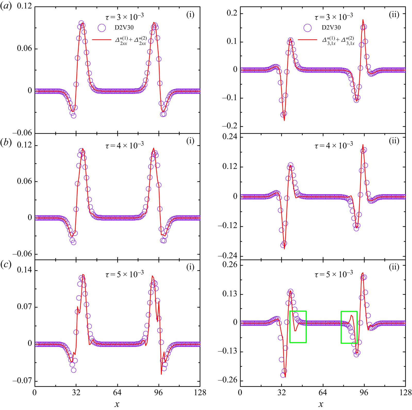
Figure 10. Effects of relaxation time on typical TNE manifestations: viscous stress (left column) and heat flux (right column).
Apart from the relative TNE intensity  $R_{{TNE}}=|\boldsymbol {\varDelta }_{m,n}^{\ast (j+1)}/\boldsymbol {\varDelta }_{m,n}^{\ast (\kern0.06em j)}|$, the aforementioned TNE discrepancy between DBM simulation and theoretical solution,
  $\boldsymbol { \varkappa }_{{Dis}}=\boldsymbol {\varDelta }^{\ast }_{{DBM}}-\boldsymbol {\varDelta }^{\ast }_{{Exact}}$, or the relative TNE discrepancy
  $R_{{Dis}}=|(\boldsymbol {\varDelta }^{\ast }_{{DBM}}-\boldsymbol {\varDelta }^{\ast }_{{Exact}})/\boldsymbol {\varDelta }^{\ast }_{{Exact}}|$ can be regarded as a non-equilibrium criterion for assessing the effectiveness of a coarse-grained model and appropriateness of the coarse-graining process, as shown in § 2. In real simulations, only when
  $R_{{TNE}}$ or
  $R_{{Dis}}$ is negligibly small is the proposed DBM physically sufficient and appropriate. Otherwise, a higher-order DBM that considers higher-order TNE effects should be adopted. Thus from this point of view, the critical relaxation time for the D2V30 model is
  $\tau _{C}=4\times 10^{-3}$ with respect to this standard test. When
  $\tau >\tau _{C}$, the present model is ineffective and unacceptable, and contributions of high-order departures from equilibrium distribution function
  $f^{(\kern0.06em j)}$ (
 $j>2$) should be considered in physical modelling.
Figure 11 further demonstrates that higher-order constitutive relations are necessary for obtaining accurate hydrodynamic quantities and fine structures of material and mechanical interfaces as the degree of non-equilibrium deepens ( $\tau =4\times 10^{-3}$), where
  $\varphi _{M}-\varphi _{N}$ represents the hydrodynamic quantity difference calculated from models with
  $M$ and
  $N$ discrete velocities. The maximum relative error in the velocity profile is
  $28.4\,\%$ at this moment, typically located at the highly non-equilibrium regime, but quickly reaches up to
  $70.0\,\%$ after
  $200$ iterations with the accumulation of errors. This kind of error, belonging to the physical modelling aspect, cannot be reduced or eliminated by improving the accuracy of the algorithm. The inaccuracy of the D2V13 and D2V15 models is due to the crucial missing of some necessary higher-order moments required for recovering
  $f^{(\kern0.06em j)}$ (
 $\kern0.06em j\geq 2$).
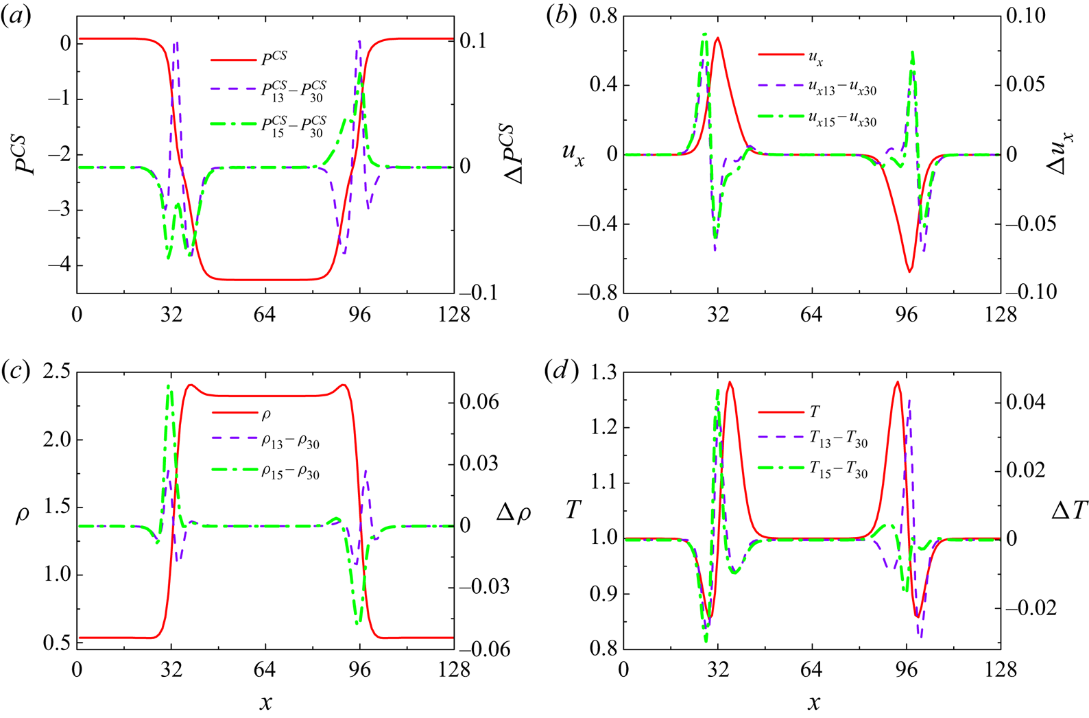
Figure 11. Hydrodynamic quantities calculated from the D2V30 model, and the corresponding differences among the D2V30, D2V15 and D2V13 models at  $t=0.01$ when
  $\tau =4\times 10^{-3}$.
Subsequently, we illustrate the effects of relaxation time on the slowly and quickly varying variables in figure 12. Figures 12(a,b) demonstrate how relaxation time  $\tau$ affects the maximum viscous stress
  $\varDelta _{2xx{-max }}^{\ast }$ and the maximum heat flux
  $\varDelta _{3,1x{-max }}^{\ast }$. Clearly,
  $\tau$ strengthens the intensities of
  $\varDelta _{2xx{-max }}^{\ast }$ and
  $\varDelta _{3,1x{-max }}^{\ast }$ in the same manner. The relationship between
  $\varDelta _{2xx{-max }}^{\ast }$ (
 $\varDelta _{3,1x{-max }}^{\ast }$) and
  $\tau$ can be divided into two stages: linear and nonlinear. When
  $\tau \leq \tau _{0}$,
  $\varDelta _{2xx{-max } }^{\ast }$ (
 $\varDelta _{3,1x{-max }}^{\ast }$) increases linearly with
  $\tau$,
  $\varDelta _{2xx{{-max}}}^{\ast }=B_{2}\tau$ (
 $\varDelta _{3,1x{{-max } }}^{\ast }=B_{4}\tau )$; when
  $\tau >\tau _{0}$, the linearization is no longer valid, and the dependence of
  $\varDelta _{2xx{-max }}^{\ast }$ (
 $\varDelta _{3,1x{-max }}^{\ast }$) on
  $\tau$ can be fitted by
  $\varDelta _{2xx{-max }}^{\ast }=A_{1}+B_{1}\tau ^{2/3}$ (
 $\varDelta _{3,1x{-max }}^{\ast }=A_{3}+B_{3}\tau ^{2/3}$), manifesting the necessity of higher-order constitutive relations for a system far away from equilibrium. The fitting parameters are
  $A_1=-0.006$,
  $B_1=4.889$,
  $B_2=45.000$,
  $A_3=-0.014$,
  $B_3=8.231$ and
  $B_4=69.291$. Of course, the ending point of the linear constitutive relations provides a distinct criterion to identify whether the system is near or far from equilibrium. Figure 12(c) shows distributions of the local Knudsen number
  $Kn(x)$ with various
  $\tau$. Similar to the behaviours of THNE,
  $Kn(x)$ becomes more pronounced in the interfacial region, and reaches its maximum at the point at which the gradient of quantity attains its peak value; it vanishes exponentially in the bulk of the liquid and vapour regions. The maximum interface Knudsen number
  $Kn_{max }$ calculated from density exceeds
  $1/3$, indicating that the D2V30 model is valid in the transition flow regime. Different from the ideal gas system and the effects of surface tension, the relaxation time
  $\tau$ only enlarges the amplitude of
  $Kn$, but does not extend the non-equilibrium region, or broaden the characteristic length scale of a system, resulting in the approximately linear dependence of
  $Kn_{max }(\rho, T,P^{cs},u_{x})$ on
  $\tau$, as shown in figure 12(d). This is because the slowly varying variables appear to be slightly affected (for
  $u_{x}(x)$, see the legend of figure 12d) or basically unaffected (for
  $\rho (x)$,
  $T(x)$,
  $P^{CS}(x)$, not shown here) by relaxation time until this moment, but noteworthily smoothed by the surface tension coefficient (see figures 13c,d). From this perspective, the interface Knudsen number calculated from the slowly varying quantity cannot be viewed as a qualified parameter to characterize the non-equilibrium behaviours at the early stage of phase separation.
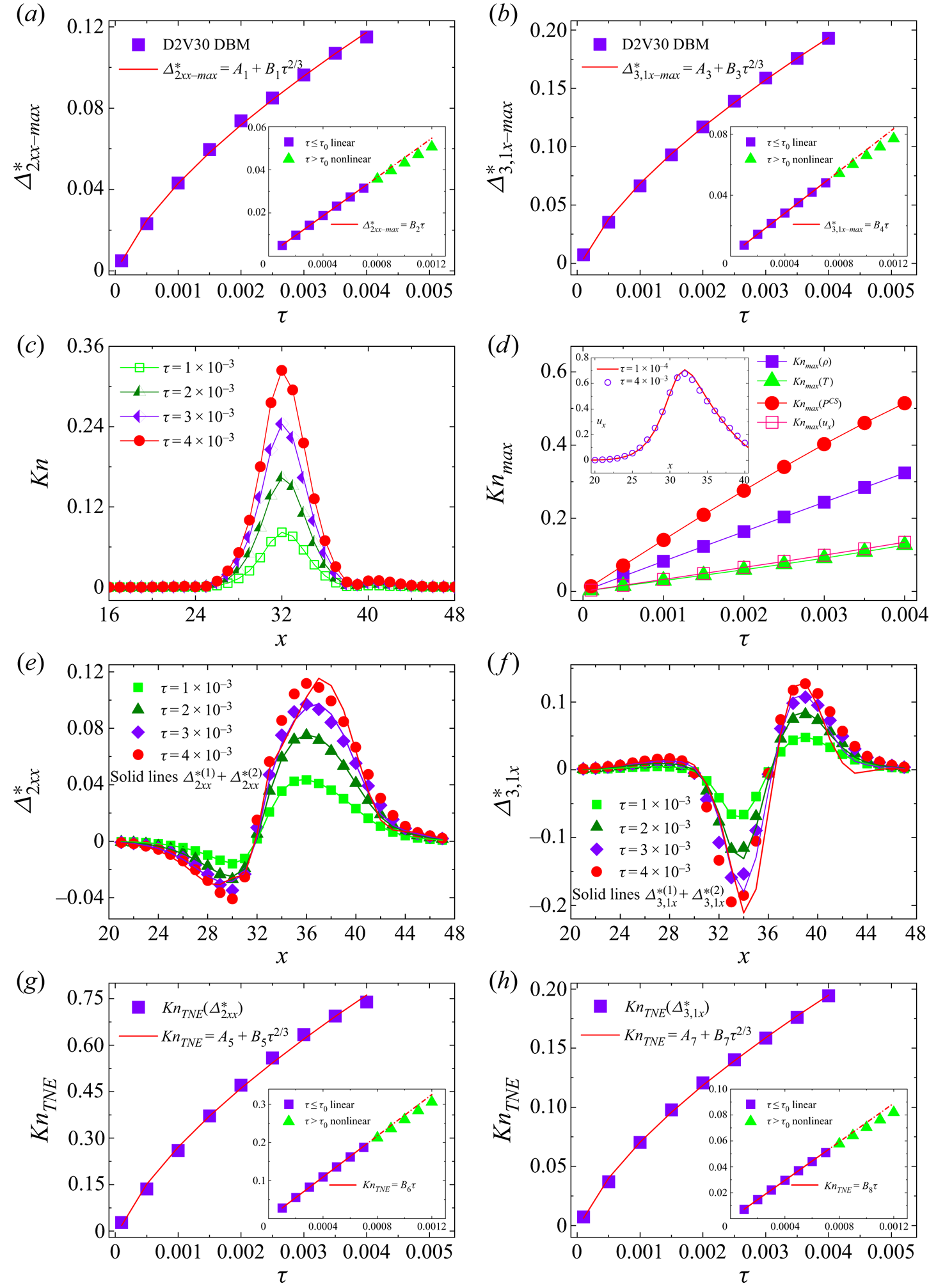
Figure 12. Effects of relaxation time on the maximum viscous stress (a), the maximum heat flux (b), distributions of the local Knudsen number (c), the maximum Knudsen number (d), distributions of viscous stress (e), distributions of heat flux ( f), the Knudsen number calculated from viscous stress (g), and the Knudsen number calculated from heat flux (h).
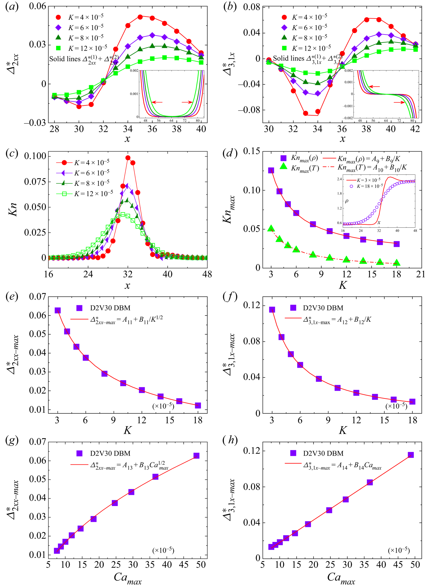
Figure 13. Effects of surface tension coefficient on the distributions of viscous stress (a), heat flux (b), the local Knudsen number (c), the maximum of Knudsen numbers calculated from density and temperature (d), the maximum viscous stress (e), and the maximum heat flux ( f). Also, the relation between the maximum viscous stress and the maximum Capillary number (g), and the relation between the maximum heat flux and the maximum Capillary number (h).
To solve this issue, we therefore resort to the quickly varying quantities, i.e. the TNE measures, and Knudsen numbers calculated from them. Figures 12(e) and 12( f) show effects of the relaxation time on viscous stresses and heat fluxes, where symbols represent DBM simulation results, and solid lines indicate the corresponding theoretical estimates. As shown in figures 12(e,f), the relaxation time substantially improves the magnitudes of TNE measures and changes their structures. The characteristic length scales are extraordinarily sensitive to relaxation time, position and time. Figures 12(g,h) suggest that the relaxation time significantly enhances the maximum Knudsen numbers calculated from viscous stress,  $Kn_{max }(\varDelta _{2xx}^{\ast })$ (figure 12g), and heat flux,
  $Kn_{max }(\varDelta _{3,1x}^{\ast })$ (figure 12h). The
  $Kn_{{TNE}}\sim \tau$ relation behaves qualitatively similarly to the one between
  $\varDelta _{2xx{-max }}^{\ast }$ (
 $\varDelta _{3,1x{-max }}^{\ast }$) and
  $\tau$. The moderate growth in
  $Kn_{{TNE}}$ when
  $\tau >\tau _{0}$ results from the second-order TNE effect that restrains the total TNE intensity.
3.4. Effects of surface tension on TNE
Here, the focus is on how and to what extent surface tension affects the dynamic patterns and TNE features. Figures 13(a) and 13(b) show the viscous stresses and heat fluxes at  $t=0.01$ for cases with various surface tension coefficients
  $K$, where symbols stand for simulation results, and solid lines represent the corresponding second-order analytical solutions. The initial conditions and other parameters are the same as those in figure 9. As shown, the surface tension effects are threefold, restraining the local TNE intensity near the interface, but expanding the TNE range and strengthening the TNE intensity away from the interface (see the solid lines and the red arrows in legends for details), through interface smoothing and extending. This result can also be verified by figures 13(c,d), where the maximum of
  $Kn$ decreases but the region with non-zero
  $Kn$ increases with
  $K$, as a result of the capillary wave broadening. When
  $K$ varies in the interval
  $[3\times 10^{-5}$,
  $18\times 10^{-5}]$, the dependence of
  $Kn_{max }(\rho )$ and
  $Kn_{max }(T)$ on
  $K$ can be fitted by
  $Kn_{max }(\rho )=A_{9}+B_{9}/K$ and
  $Kn_{max }(T)=A_{10}+B_{10}/K$, respectively, with
  $A_{9}=0.013$,
  $B_9=3.422\times 10^{-6}$,
  $A_{10}=-0.003$, and
  $B_{10}=1.588\times 10^{-6}$. The high sensitivity of density profile to surface tension coefficient (see the legend of figure 13d) is due mainly to the
  $\boldsymbol {\varLambda }$ term in (2.2) that is linearly proportional to
  $K$.
$K$.
Accordingly, as plotted in figures 13(e, f), the maxima of  $\varDelta _{2xx}^{\ast }$ and
  $\varDelta _{3,1x}^{\ast }$ decrease synchronously with
  $K$ approximately as
  $\varDelta _{2xx{{-max}}}^{\ast }=A_{11}+B_{11}/K^{1/2}$ and
  $\varDelta _{3,1{{-max }} }^{\ast }=A_{12}+B_{12}/K$, with
  $A_{11}=-0.023$,
  $B_{11}=4.667\times 10^{-4}$,
  $A_{12}=0.008$ and
  $B_{12}=3.711\times 10^{-6}$. In other words, large resistances to mass and heat transfers appear at the interface, and increase with the surface tension coefficient. The suppressive effect of surface tension on heat flux is much stronger than that on viscous stress at a small Prandtl number. We further examine the effects of surface tension on TNE in terms of the capillary number
  $Ca$, which denotes the ratio between viscous force and interfacial tension,
  $Ca=\mu u_{C}/\sigma$, with
  $u_{C}$ the characteristic velocity, and
  $\sigma$ the interfacial tension between liquid and vapour phases. For a planar interface,
  $\sigma$ can be computed specifically as
  $\sigma =K\int _{-\infty }^{\infty }({\partial \rho }/{\partial z})^{2}\, \textrm {d} z$. Figures 13(g,h) show relations among TNE measures and the maximum capillary number
  $Ca_{{max}}$. Clearly,
  $\varDelta _{2xx{{-max}}}^{\ast }$ and
  $\varDelta _{3,1x{{-max}}}^{\ast }$ increase with increasing
  $Ca_{{max}}$. The two relations can be fitted by
  $\varDelta _{2xx{{-max} }}^{\ast }=A_{13}+B_{13}\,Ca_{{max}}^{1/2}$ and
  $\varDelta _{3,1{{-max } }}^{\ast }=A_{14}+B_{14}\,Ca_{{max}}$, with fitting parameters
  $A_{13}=-0.021$,
  $B_{13}=3.761$,
  $A_{14}=-0.007$ and
  $B_{14}=249.513$. The diametrically opposite trends in figures 13(e) and 13(g) (also figures 13( f,h)) are due to the inverse relation between
  $Ca_{{max}}$ and
  $K$,
$K$,  $Ca_{{max}}\sim K^{-1}$.
4. Conclusions and remarks
From the perspective of kinetic theory, the transport properties of a flowing system are described by the distribution function  $f$ or by the full sequence of its kinetic moments. The conservative kinetic moments of
  $f$ include the density, momentum and energy. Acquisition of these conservative kinetic moments is equivalent to knowing only the equilibrium distribution function
  $f^{(0)}$, namely perfect fluids free from dissipative effects. How and to what extent the system deviates from the thermodynamic equilibrium remains completely unknown at this stage.
To know the distribution function  $f$ is equivalent to knowing all the kinetic moments of
  $f$, which is neither possible nor necessary for the vast majority of situations. Which kinetic moments need to be known for multi-scale modelling of complex flows is the first key question that the DBM endeavours to address. The second is how to detect, describe, present and analyse THNE states. Along this line, we present a framework for constructing multi-scale discrete Boltzmann models for thermal multiphase flows ranging from continuum to transition flow regimes. The DBM is a straightforward and efficient kinetic moment-matching method, for bulk flow, whose basic framework consists of three fundamental steps: (i) establishment of the formal links with the modified continuous Boltzmann–BGK equation, the extended hydrodynamic equations and the sought thermo-hydrodynamic non-equilibrium (THNE) phenomena under consideration; (ii) formulation of the THNE measures; and (iii) discretization of the particle velocity space for the construction of the discrete equilibrium distribution function. In addition, phase space manifolds spanned by the independent components of non-conservative kinetic moments of
  $(f-f^{(0)})$ are introduced to describe the corresponding non-equilibrium states and effects. The concept of metric distance from the origin in such phase space is extended to describe intuitively the non-equilibrium depth. The concept of metric distance between two points in such phase space is extended to describe intuitively the difference between two states. For near-wall flow, one more step, construction of kinetic boundary conditions, is needed.
In the case of the validity of Chapman–Enskog theory, step (ii) permits us to select the minimum physical requirements for describing the THNE quantities of interest to the desired order of accuracy, that is, it determines the fewest required kinetic moments  $\boldsymbol {\varPhi }_{n}=(\boldsymbol {M}_{0}, \boldsymbol {M}_{1}, \ldots, \boldsymbol {M} _{n})^\textrm {T}$ that the discrete equilibrium distribution function should retrieve during the coarse-grained physical modelling process. It also provides valuable byproducts: higher-order constitutive relations and the most relevant higher-order THNE manifestations that are expected to improve the macroscopic modelling and enhance the understanding of dynamic constitutive relations.
The set of the fewest kinetic moments offers a unique perspective to investigate the non-equilibrium behaviour of the ‘mesoscale’ or ‘dilemma’ situations where the continuum modelling fails and the molecular dynamics method lacks sufficient power to reach up to the scales of interest. The research perspective and modelling accuracy depend on the specific elements of moment sets, and can be adjusted and improved in time. For instance, to access stronger non-equilibrium effects, one needs to include more higher-order moment relations into  $\boldsymbol {\varPhi }_{n}$, so that the discrete Boltzmann model becomes more consistent with the continuous Boltzmann equation far from equilibrium. Importantly, the computational complexity of the DBM increases only mildly in the process, as opposed to the case of generalized hydrodynamics, such as the Burnett or the super-Burnett equations.
As model examples, two-dimensional discrete Boltzmann models with  $13$,
$13$,  $15$ and
  $30$ discrete velocities at Navier–Stokes and beyond Burnett levels have been proposed and evaluated. It is found that the incorporation of additional higher-order kinetic moments helps to enhance the liquid–vapour density ratio that the model can hold, to curb spurious currents around the interface, and to ensure better mass, momentum and energy conservation in phase-separating systems. The multi-scale predictive capability of the discrete Boltzmann model to describe THNE features increases with the number of independent kinetic moments included by the model. As fast-varying variables, the thermodynamic and THNE measures provide more detailed information on the non-equilibrium multiphase flow system than methods based on macroscopic conserved quantities alone, thereby shedding new light on these complex states of flowing matter far from equilibrium. For example, the present work helps in preparing the cognitive basis for subsequent experimental research, and provides theoretical guidance for further experimental design, observation and analysis.
Future work includes: a more complete comparison among DBM results, high-order moment method (Struchtrup & Frezzotti Reference Struchtrup and Frezzotti2022), particle-based method (Frezzotti et al. Reference Frezzotti, Gibelli, Lockerby and Sprittles2018, Reference Frezzotti, Barbante and Gibelli2019) and experimental results; the incorporation of the external force in a more fundamental way; the construction of appropriate kinetic boundary conditions (Struchtrup et al. Reference Struchtrup, Beckmann, Rana and Frezzotti2017; Zhang et al. Reference Zhang, Xu, Chen, Lin and Wei2022b); and consideration of the case with faster phase separation, say the phase transition time scale is comparable to the molecular thermal relaxation.
Acknowledgements
The authors sincerely thank the anonymous reviewers for their valuable and instructive comments and suggestions, which were very helpful for revising the manuscript. Also, we warmly thank Dr T. Chen (Southern University of Science and Technology), Dr Y. Zhang (Zhengzhou University), Dr C. Lin (Sun Yat-sen University), Dr D. Zhang (China University of Mining and Technology (Beijing)) and Dr B. Chen (North China Institute of Aerospace Engineering) for many helpful discussions.
Funding
We acknowledge support from the National Natural Science Foundation of China (grant nos 11875001 and 12172061), the Natural Science Foundation of Hebei Province (grant nos. A2021409001 and 226Z7601G), the ‘Three, Three and Three’ Talent Project of Hebei Province (grant no. A202105005), the Natural Science Foundation of Fujian Province (grant no. 2021J01652), the CAEP Foundation (grant no. CX2019033), the opening project of State Key Laboratory of Explosion Science and Technology (Beijing Institute of Technology) (grant no. KFJJ21-16M) and the Foundation of Laboratory of Computational Physics. S.S. gratefully acknowledges financial support from the European Research Council under the Horizon 2020 Programme Grant Agreement no. 739964 (‘COPMAT’).
Declaration of interests
The authors report no conflict of interest.
Appendix A. Determination of the relations among THNE and TNE measures
According to the definitions in (2.9) and (2.10),  $\boldsymbol {\varDelta }_{m,n}$ describes the combination effects of thermodynamic non-equilibrium (TNE) and hydrodynamic non-equilibrium (HNE), which are usually called the thermo-hydrodynamic non-equilibrium (THNE) effects;
  $\boldsymbol {\varDelta }_{m,n}^{\ast }$ reflects molecular individualism on top of organized collective motion, describing only the TNE effects. Next, we list the relations among them:
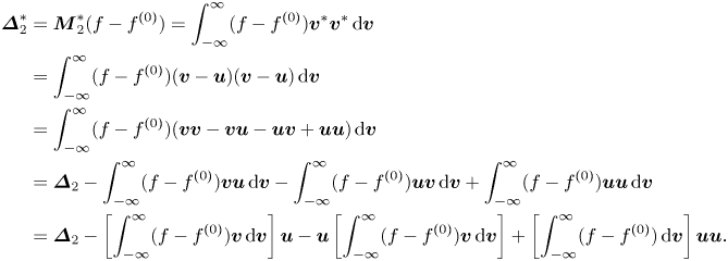 \begin{align} \boldsymbol{\varDelta}_{2}^{{\ast} } &= \boldsymbol{M}_{2}^{{\ast} }(f-f^{(0)})=\int_{-\infty }^{\infty }(f-f^{(0)}){\boldsymbol{v}}^{{\ast} }{\boldsymbol{v}}^{{\ast} }\, {\rm d} \boldsymbol{v} \nonumber\\ &= \int_{-\infty }^{\infty }(f-f^{(0)})({\boldsymbol{v}}-{\boldsymbol{u}})({\boldsymbol{v }}-{\boldsymbol{u}})\, {\rm d} \boldsymbol{v} \nonumber\\ &= \int_{-\infty }^{\infty }(f-f^{(0)})({\boldsymbol{vv}}-{\boldsymbol{vu}-\boldsymbol{uv}+\boldsymbol{uu}})\, {\rm d} \boldsymbol{v} \nonumber\\ &= \boldsymbol{\varDelta}_{2}-\int_{-\infty }^{\infty }(f-f^{(0)}){\boldsymbol{vu}}\, {\rm d} \boldsymbol{ v}-\int_{-\infty }^{\infty }(f-f^{(0)}){\boldsymbol{uv}}\, {\rm d} \boldsymbol{v}+ \int_{-\infty }^{\infty }(f-f^{(0)}){\boldsymbol{uu}}\, {\rm d} \boldsymbol{v} \nonumber\\ &= \boldsymbol{\varDelta}_{2}-\left[\int_{-\infty }^{\infty }(f-f^{(0)}){\boldsymbol{v}}\, {\rm d} \boldsymbol{v}\right] \boldsymbol{u}-\boldsymbol{u}\left[\int_{-\infty }^{\infty }(f-f^{(0)}){\boldsymbol{v}}\, {\rm d} \boldsymbol{v}\right]+ \left[\int_{-\infty}^{\infty }(f-f^{(0)})\, {\rm d} \boldsymbol{v} \right]{\boldsymbol{uu}}. \end{align}
It is well known that  $\int _{-\infty }^{\infty }(f-f^{(0)})\, \textrm {d} \boldsymbol {v}=0$ and
  $\int _{-\infty }^{\infty }(f-f^{(0)}){\boldsymbol {v}}\, \textrm {d} \boldsymbol {v}=0$, so
 \begin{equation} \boldsymbol{\varDelta}_{2}^{{\ast} }=\boldsymbol{\varDelta}_{2}. \end{equation}
We have
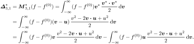 \begin{align} \boldsymbol{\varDelta}_{3,1}^{{\ast} } &= \boldsymbol{M}_{3,1}^{{\ast} }(f-f^{(0)})=\int_{-\infty }^{\infty }(f-f^{(0)}){\boldsymbol{v}}^{{\ast} }\,\frac{{ \boldsymbol{v}}^{{\ast} }\boldsymbol{\cdot} {\boldsymbol{v}}^{{\ast} }}{2}\, {\rm d} \boldsymbol{v} \nonumber\\ &= \int_{-\infty }^{\infty }(f-f^{(0)})({\boldsymbol{v}}-{\boldsymbol{u}})\,\frac{ v^{2}-2{\boldsymbol{v}}\boldsymbol{\cdot} {\boldsymbol{u}}+u^{2}}{2}\, {\rm d} \boldsymbol{v} \nonumber\\ &= \int_{-\infty }^{\infty }(f-f^{(0)}){\boldsymbol{v}}\,\frac{v^{2}-2{\boldsymbol{v}} \boldsymbol{\cdot} {\boldsymbol{u}}+u^{2}}{2}\, {\rm d} \boldsymbol{v}-\int_{-\infty }^{\infty }(f-f^{(0)}){ \boldsymbol{u}}\,\frac{v^{2}-2{\boldsymbol{v}}\boldsymbol{\cdot} {\boldsymbol{u}}+u^{2}}{2}\, {\rm d} \boldsymbol{v}. \end{align}
It is clear that  $\int _{-\infty }^{\infty }(f-f^{(0)})({v^{2}}/{2})\, \textrm {d} \boldsymbol {v}=0$, hence
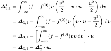 \begin{align}\boldsymbol{\varDelta}_{3,1}^{{\ast} } &= \int_{-\infty}^{\infty}(f-f^{(0)}){\boldsymbol{v}}\left(\frac{v^{2}}{2}-{\boldsymbol{v}}\boldsymbol{\cdot}{\boldsymbol{u}}+\frac{u^{2}}{2}\right)\, {\rm d}\boldsymbol{v}\nonumber\\ &=\boldsymbol{\varDelta}_{3,1}-\int_{-\infty }^{\infty}(f-f^{(0)}){\boldsymbol{v}}\left({\boldsymbol{v}}\boldsymbol{\cdot}{\boldsymbol{u}}-\frac{u^{2}}{2}\right)\, {\rm d}\boldsymbol{v} \nonumber\\ &=\boldsymbol{\varDelta}_{3,1}-\left[\int_{-\infty }^{\infty}(f-f^{(0)}){\boldsymbol{vv}}\, {\rm d}\boldsymbol{v}\right]\boldsymbol{\cdot} {\boldsymbol{u}}\nonumber\\ &=\boldsymbol{\varDelta}_{3,1}-\boldsymbol{\varDelta}_{2}^{{\ast}}\boldsymbol{\cdot} {\boldsymbol{u}}.\end{align}
Similarly,
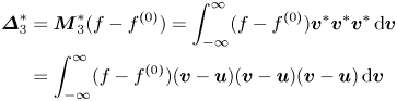 \begin{align}
\boldsymbol{\varDelta}_{3}^{{\ast} } &=
\boldsymbol{M}_{3}^{{\ast} }(f-f^{(0)})=\int_{-\infty
}^{\infty }(f-f^{(0)}){\boldsymbol{v}}^{{\ast}
}{\boldsymbol{v}}^{{\ast} }{\boldsymbol{v}} ^{{\ast} }\,
{\rm d} \boldsymbol{v} \nonumber\\ &=\int_{-\infty
}^{\infty}(f-f^{(0)})({\boldsymbol{v}}-{\boldsymbol{u}})({
\boldsymbol{v}}-{\boldsymbol{u}})({\boldsymbol{v}}-{\boldsymbol{u}})\,
{\rm d} \boldsymbol{v} \nonumber\\ &= \int_{-\infty
}^{\infty
}(f-f^{(0)})({\boldsymbol{vvv}}-{\boldsymbol{vuv}}-{
\boldsymbol{uvv}}+{\boldsymbol{uuv}-\boldsymbol{vvu}+\boldsymbol{vuu}+\boldsymbol{u{v}u}-\boldsymbol{uuu}})\,
{\rm d} \boldsymbol{v} \nonumber\\ &=
\int_{-\infty }^{\infty
}(f-f^{(0)})({\boldsymbol{vvv}}-{\boldsymbol{vuv}}-{
\boldsymbol{uvv}-\boldsymbol{vvu}})\, {\rm d}
\boldsymbol{v} \nonumber\\ &=
\boldsymbol{\varDelta}_{3}-\int_{-\infty }^{\infty
}(f-f^{(0)})({\boldsymbol{vuv}}+
\boldsymbol{uvv}+\boldsymbol{vvu})\, {\rm d}
\boldsymbol{v} \nonumber\\ &=
\boldsymbol{\varDelta}_{3}-\int_{-\infty }^{\infty
}(f-f^{(0)}){\boldsymbol{vuv}}\, {\rm d}
\boldsymbol{v}-{\boldsymbol{u}}\boldsymbol{\varDelta}_{2}^{{\ast}
}-\boldsymbol{\varDelta}_{2}^{{\ast} }{ \boldsymbol{u}}
\nonumber\\ &= \boldsymbol{\varDelta}_{3}-(u_{\alpha
}\varDelta_{2\beta \gamma }^{{\ast} }+u_{\beta
}\varDelta_{2\alpha \gamma }^{{\ast} }+u_{\gamma
}\varDelta_{2\alpha \beta }^{{\ast}
})\boldsymbol{e}_{\alpha }\boldsymbol{e}_{\beta
}\boldsymbol{e}_{\gamma} \end{align}
\begin{align}
\boldsymbol{\varDelta}_{3}^{{\ast} } &=
\boldsymbol{M}_{3}^{{\ast} }(f-f^{(0)})=\int_{-\infty
}^{\infty }(f-f^{(0)}){\boldsymbol{v}}^{{\ast}
}{\boldsymbol{v}}^{{\ast} }{\boldsymbol{v}} ^{{\ast} }\,
{\rm d} \boldsymbol{v} \nonumber\\ &=\int_{-\infty
}^{\infty}(f-f^{(0)})({\boldsymbol{v}}-{\boldsymbol{u}})({
\boldsymbol{v}}-{\boldsymbol{u}})({\boldsymbol{v}}-{\boldsymbol{u}})\,
{\rm d} \boldsymbol{v} \nonumber\\ &= \int_{-\infty
}^{\infty
}(f-f^{(0)})({\boldsymbol{vvv}}-{\boldsymbol{vuv}}-{
\boldsymbol{uvv}}+{\boldsymbol{uuv}-\boldsymbol{vvu}+\boldsymbol{vuu}+\boldsymbol{u{v}u}-\boldsymbol{uuu}})\,
{\rm d} \boldsymbol{v} \nonumber\\ &=
\int_{-\infty }^{\infty
}(f-f^{(0)})({\boldsymbol{vvv}}-{\boldsymbol{vuv}}-{
\boldsymbol{uvv}-\boldsymbol{vvu}})\, {\rm d}
\boldsymbol{v} \nonumber\\ &=
\boldsymbol{\varDelta}_{3}-\int_{-\infty }^{\infty
}(f-f^{(0)})({\boldsymbol{vuv}}+
\boldsymbol{uvv}+\boldsymbol{vvu})\, {\rm d}
\boldsymbol{v} \nonumber\\ &=
\boldsymbol{\varDelta}_{3}-\int_{-\infty }^{\infty
}(f-f^{(0)}){\boldsymbol{vuv}}\, {\rm d}
\boldsymbol{v}-{\boldsymbol{u}}\boldsymbol{\varDelta}_{2}^{{\ast}
}-\boldsymbol{\varDelta}_{2}^{{\ast} }{ \boldsymbol{u}}
\nonumber\\ &= \boldsymbol{\varDelta}_{3}-(u_{\alpha
}\varDelta_{2\beta \gamma }^{{\ast} }+u_{\beta
}\varDelta_{2\alpha \gamma }^{{\ast} }+u_{\gamma
}\varDelta_{2\alpha \beta }^{{\ast}
})\boldsymbol{e}_{\alpha }\boldsymbol{e}_{\beta
}\boldsymbol{e}_{\gamma} \end{align}and
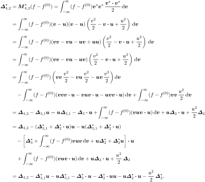 \begin{align}
\boldsymbol{\varDelta}_{4,2}^{{\ast} } &=
\boldsymbol{M}_{4,2}^{{\ast} }(f-f^{(0)})=\int_{-\infty
}^{\infty }(f-f^{(0)}){\boldsymbol{v}}^{{\ast} }{
\boldsymbol{v}}^{{\ast} }\,\frac{{\boldsymbol{v}}^{{\ast}
}\boldsymbol{\cdot} {\boldsymbol{v}}^{{\ast} }}{2}\, {\rm d} \boldsymbol{v} \nonumber\\
& = \int_{-\infty }^{\infty
}(f-f^{(0)})({\boldsymbol{v}}-{\boldsymbol{u}})({
\boldsymbol{v}}-{\boldsymbol{u}})\left(\frac{v^{2}}{2}-{\boldsymbol{v}}\boldsymbol{\cdot}
{\boldsymbol{u}}+\frac{u^{2}}{2}\right)\, {\rm d} \boldsymbol{v} \nonumber\\
& = \int_{-\infty }^{\infty }(f-f^{(0)})({\boldsymbol{vv}}-{\boldsymbol{
vu}-\boldsymbol{uv}+\boldsymbol{uu}})
\left(\frac{v^{2}}{2}-{\boldsymbol{v}}\boldsymbol{\cdot}
{\boldsymbol{u}}+\frac{u^{2}}{2}\right)\, {\rm d} \boldsymbol{v} \nonumber\\
&= \int_{-\infty }^{\infty }(f-f^{(0)})({\boldsymbol{vv}}-{\boldsymbol{vu}-\boldsymbol{uv}})
\left(\frac{v^{2}}{2}-{\boldsymbol{v}}\boldsymbol{\cdot}
{\boldsymbol{u}}+\frac{u^{2}}{2}\right)\, {\rm d}
\boldsymbol{v} \nonumber\\
&= \int_{-\infty }^{\infty }(f-f^{(0)}) \left({\boldsymbol{vv}}\,\frac{v^{2}}{2}-{
\boldsymbol{vu}}\,\frac{v^{2}}{2}-{\boldsymbol{uv}}\,\frac{v^{2}}{2}\right)
{\rm d} \boldsymbol{v} \nonumber\\
&\quad -\int_{-\infty }^{\infty }(f-f^{(0)})({\boldsymbol{vvv}}\boldsymbol{\cdot}
{\boldsymbol{u}}-{\boldsymbol{vuv}\boldsymbol{\cdot}
\boldsymbol{u}-\boldsymbol{uvv}}\boldsymbol{\cdot}
{\boldsymbol{u}})\, {\rm d} \boldsymbol{v}
+\int_{-\infty}^{\infty }(f-f^{(0)}){\boldsymbol{vv}}\,
\frac{u^{2}}{2}\, {\rm d} \boldsymbol{v} \nonumber\\
&=\boldsymbol{\varDelta}_{4,2}-\boldsymbol{\varDelta}_{3,1}
{\boldsymbol{u-u}}\boldsymbol{\varDelta}_{3,1}-
\boldsymbol{\varDelta}_{3}\boldsymbol{\cdot}
{\boldsymbol{u}}+ \!\int_{-\infty }^{\infty}(f-f^{(0)}) ({
\boldsymbol{vu{\boldsymbol{v}}\boldsymbol{\cdot}
{\boldsymbol{u}}}})\, {\rm d} \boldsymbol{v}+
{\boldsymbol{u}}\boldsymbol{\varDelta}_{2}\boldsymbol{\cdot}
{\boldsymbol{u}}+\frac{u^{2}}{2} \boldsymbol{\varDelta}_{2}
\nonumber\\ &=
\boldsymbol{\varDelta}_{4,2}-(\boldsymbol{\varDelta}_{3,1}^{{\ast}
}+\boldsymbol{\varDelta}_{2}^{{\ast} }\boldsymbol{\cdot}
{\boldsymbol{u}}){\boldsymbol{u}}-\boldsymbol{u}(\boldsymbol{\varDelta}_{3,1}^{{\ast}
}+\boldsymbol{\varDelta}_{2}^{{\ast} }\boldsymbol{\cdot}
{\boldsymbol{u}}) \nonumber\\ &\quad
-\left[\boldsymbol{\varDelta}_{3}^{{\ast} }+\int_{-\infty
}^{\infty }(f-f^{(0)}){\boldsymbol{vuv} }\, {\rm d}
\boldsymbol{v}+{\boldsymbol{u}}\boldsymbol{\varDelta}_{2}^{{\ast}
}+\boldsymbol{\varDelta}_{2}^{{\ast} }{
\boldsymbol{u}}\right]\boldsymbol{\cdot} {\boldsymbol{u}}
\nonumber\\ &\quad +\int_{-\infty }^{\infty
}(f-f^{(0)})(\boldsymbol{vuv} \boldsymbol{\cdot}
\boldsymbol{u})\, {\rm d}
\boldsymbol{v}+{\boldsymbol{u}}\boldsymbol{\varDelta}_{2}\boldsymbol{\cdot}
{\boldsymbol{u}}+\frac{u^{2}}{2}\,\boldsymbol{\varDelta}_{2}
\nonumber\\ &=
\boldsymbol{\varDelta}_{4,2}-\boldsymbol{\varDelta}_{3,1}^{{\ast}}
{\boldsymbol{u}-\boldsymbol{u}}\boldsymbol{\varDelta}
_{3,1}^{{\ast}} -\boldsymbol{\varDelta}_{3}^{{\ast}
}\boldsymbol{\cdot} {\boldsymbol{u}}-\boldsymbol{\varDelta}
_{2}^{{\ast} }\boldsymbol{\cdot}
{\boldsymbol{uu}}-\boldsymbol{u}\boldsymbol{\varDelta}_{2}^{{\ast}}
\boldsymbol{\cdot}
{\boldsymbol{u}}-
\frac{u^{2}}{2}\,\boldsymbol{\varDelta}_{2}^{{\ast}}.
\end{align}
\begin{align}
\boldsymbol{\varDelta}_{4,2}^{{\ast} } &=
\boldsymbol{M}_{4,2}^{{\ast} }(f-f^{(0)})=\int_{-\infty
}^{\infty }(f-f^{(0)}){\boldsymbol{v}}^{{\ast} }{
\boldsymbol{v}}^{{\ast} }\,\frac{{\boldsymbol{v}}^{{\ast}
}\boldsymbol{\cdot} {\boldsymbol{v}}^{{\ast} }}{2}\, {\rm d} \boldsymbol{v} \nonumber\\
& = \int_{-\infty }^{\infty
}(f-f^{(0)})({\boldsymbol{v}}-{\boldsymbol{u}})({
\boldsymbol{v}}-{\boldsymbol{u}})\left(\frac{v^{2}}{2}-{\boldsymbol{v}}\boldsymbol{\cdot}
{\boldsymbol{u}}+\frac{u^{2}}{2}\right)\, {\rm d} \boldsymbol{v} \nonumber\\
& = \int_{-\infty }^{\infty }(f-f^{(0)})({\boldsymbol{vv}}-{\boldsymbol{
vu}-\boldsymbol{uv}+\boldsymbol{uu}})
\left(\frac{v^{2}}{2}-{\boldsymbol{v}}\boldsymbol{\cdot}
{\boldsymbol{u}}+\frac{u^{2}}{2}\right)\, {\rm d} \boldsymbol{v} \nonumber\\
&= \int_{-\infty }^{\infty }(f-f^{(0)})({\boldsymbol{vv}}-{\boldsymbol{vu}-\boldsymbol{uv}})
\left(\frac{v^{2}}{2}-{\boldsymbol{v}}\boldsymbol{\cdot}
{\boldsymbol{u}}+\frac{u^{2}}{2}\right)\, {\rm d}
\boldsymbol{v} \nonumber\\
&= \int_{-\infty }^{\infty }(f-f^{(0)}) \left({\boldsymbol{vv}}\,\frac{v^{2}}{2}-{
\boldsymbol{vu}}\,\frac{v^{2}}{2}-{\boldsymbol{uv}}\,\frac{v^{2}}{2}\right)
{\rm d} \boldsymbol{v} \nonumber\\
&\quad -\int_{-\infty }^{\infty }(f-f^{(0)})({\boldsymbol{vvv}}\boldsymbol{\cdot}
{\boldsymbol{u}}-{\boldsymbol{vuv}\boldsymbol{\cdot}
\boldsymbol{u}-\boldsymbol{uvv}}\boldsymbol{\cdot}
{\boldsymbol{u}})\, {\rm d} \boldsymbol{v}
+\int_{-\infty}^{\infty }(f-f^{(0)}){\boldsymbol{vv}}\,
\frac{u^{2}}{2}\, {\rm d} \boldsymbol{v} \nonumber\\
&=\boldsymbol{\varDelta}_{4,2}-\boldsymbol{\varDelta}_{3,1}
{\boldsymbol{u-u}}\boldsymbol{\varDelta}_{3,1}-
\boldsymbol{\varDelta}_{3}\boldsymbol{\cdot}
{\boldsymbol{u}}+ \!\int_{-\infty }^{\infty}(f-f^{(0)}) ({
\boldsymbol{vu{\boldsymbol{v}}\boldsymbol{\cdot}
{\boldsymbol{u}}}})\, {\rm d} \boldsymbol{v}+
{\boldsymbol{u}}\boldsymbol{\varDelta}_{2}\boldsymbol{\cdot}
{\boldsymbol{u}}+\frac{u^{2}}{2} \boldsymbol{\varDelta}_{2}
\nonumber\\ &=
\boldsymbol{\varDelta}_{4,2}-(\boldsymbol{\varDelta}_{3,1}^{{\ast}
}+\boldsymbol{\varDelta}_{2}^{{\ast} }\boldsymbol{\cdot}
{\boldsymbol{u}}){\boldsymbol{u}}-\boldsymbol{u}(\boldsymbol{\varDelta}_{3,1}^{{\ast}
}+\boldsymbol{\varDelta}_{2}^{{\ast} }\boldsymbol{\cdot}
{\boldsymbol{u}}) \nonumber\\ &\quad
-\left[\boldsymbol{\varDelta}_{3}^{{\ast} }+\int_{-\infty
}^{\infty }(f-f^{(0)}){\boldsymbol{vuv} }\, {\rm d}
\boldsymbol{v}+{\boldsymbol{u}}\boldsymbol{\varDelta}_{2}^{{\ast}
}+\boldsymbol{\varDelta}_{2}^{{\ast} }{
\boldsymbol{u}}\right]\boldsymbol{\cdot} {\boldsymbol{u}}
\nonumber\\ &\quad +\int_{-\infty }^{\infty
}(f-f^{(0)})(\boldsymbol{vuv} \boldsymbol{\cdot}
\boldsymbol{u})\, {\rm d}
\boldsymbol{v}+{\boldsymbol{u}}\boldsymbol{\varDelta}_{2}\boldsymbol{\cdot}
{\boldsymbol{u}}+\frac{u^{2}}{2}\,\boldsymbol{\varDelta}_{2}
\nonumber\\ &=
\boldsymbol{\varDelta}_{4,2}-\boldsymbol{\varDelta}_{3,1}^{{\ast}}
{\boldsymbol{u}-\boldsymbol{u}}\boldsymbol{\varDelta}
_{3,1}^{{\ast}} -\boldsymbol{\varDelta}_{3}^{{\ast}
}\boldsymbol{\cdot} {\boldsymbol{u}}-\boldsymbol{\varDelta}
_{2}^{{\ast} }\boldsymbol{\cdot}
{\boldsymbol{uu}}-\boldsymbol{u}\boldsymbol{\varDelta}_{2}^{{\ast}}
\boldsymbol{\cdot}
{\boldsymbol{u}}-
\frac{u^{2}}{2}\,\boldsymbol{\varDelta}_{2}^{{\ast}}.
\end{align}Appendix B. Expressions for the first- and second-order TNE measures
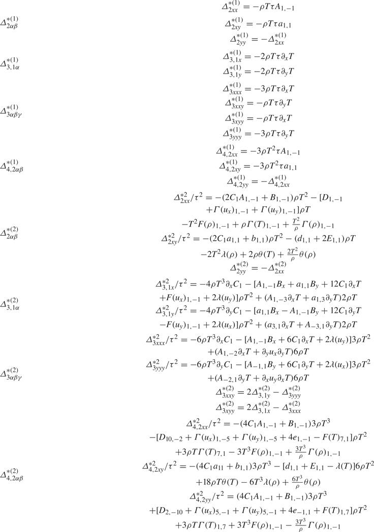
Here,  ${A_{m,n}}=m\partial _{x}{u_{x}}+n\partial _{y}{u_{y}}$,
  ${a_{m,n}} =m\partial _{x}{u_{y}}+m\partial _{y}u_{x}$,
  ${B_{m,n}}=m\partial _{x}B_{x}+n \partial _{y}B_{y}$,
  ${b_{m,n}}=m\partial _{x}B_{y}+n\partial _{y}B_{x}$,
  ${ D_{m,n}}=m{B_{x}}\partial _{x}T+n{B_{y}}\partial _{y}T$,
  ${d_{m,n}}=m{B_{y}} \partial _{x}T+n{B_{x}}\partial _{y}T$,
  ${E_{m,n}}=m\partial _{x}u_{x} \partial _{y}u_{x}+n\partial _{x}u_{y}\partial _{y}u_{y}$,
  ${e_{m,n}} =m\partial _{x}u_{x}\partial _{y}u_{y}+n\partial _{x}u_{y}\partial _{y}u_{x}$,
  $\theta (\cdot )=\partial _{x}(\cdot )\partial _{y}(\cdot )$,
  $\lambda (\cdot ) =({{{\partial ^{2}}}}/{{\partial y\partial x}})(\cdot )$,
  $F(\cdot ){_{m,n}}=m({{{\partial ^{2}}}}/{{\partial {x^{2}}}})(\cdot )+n ({{{\partial ^{2}}}}/{{\partial {y^{2}}}})(\cdot )$,
  $\varGamma (\cdot ){_{m,n}}=m[\partial _{x}(\cdot )]{^{2}} +n[\partial _{y}(\cdot )]{^{2}}$,
  $C_1=C+C_q$.
Appendix C. Independent kinetic moments required to fully characterize the first- and second-order TNE measures