


1 Introduction
As internal waves propagate, they leave on the ocean surface a distinct signature of alternating rough and smooth regions. When observed using satellite radars, this signature of internal waves appears in the form of bright and dark bands, similar to the white and black stripes of a zebra. Such bands appear because a spatial change in the wave roughness induces a variation in the strength of the backscattering of the electromagnetic signals of radars (Perry & Schimke Reference Perry and Schimke1965; Ziegenbein Reference Ziegenbein1969; Osborne & Burch Reference Osborne and Burch1980). The surface signature obtained via remote sensing is a critical technique for the identification of internal waves (Helfrich & Melville Reference Helfrich and Melville2006), which allows a large area coverage compared with in situ measurements. The heterogeneity in surface roughness can impact the physical properties of the near-surface atmosphere (Ortiz-Suslow et al. Reference Ortiz-Suslow, Wang, Kalogiros, Yamaguchi, Paolo, Terrill, Shearman, Welch and Savelyev2019). Despite its importance, it remains a challenge to quantify the surface signature induced by internal waves. It is desirable to resolve a wide range of wave motions from the first principles of fluid dynamics so that the impact of internal waves on the surface waves can be accurately described and modelled.
In previous studies, attempts to quantify the surface wave variation are often based on the ray theory, which is similar to geometrical optics. In this theory, an individual surface wave component is tracked by the change in its wavenumber and energy, whereas the wave phase is discarded. The effect of the internal wave is generally treated as a prescribed time-invariant surface current (Alpers Reference Alpers1985; Donato, Peregrine & Stocker Reference Donato, Peregrine and Stocker1999; Bakhanov & Ostrovsky Reference Bakhanov and Ostrovsky2002). Under this assumption, a singularity occurs when the surface waves are blocked by the countercurrent induced by the internal wave (Peregrine Reference Peregrine and Yih1976). The singularity can be illustrated by the dispersion relation of a one-dimensional surface wave in a current,  $\unicode[STIX]{x1D714}=kU+\sqrt{gk}$, where
  $\unicode[STIX]{x1D714}$ denotes the wave (angular) frequency,
  $k$ the wavenumber and
  $U$ the current velocity. The dispersion relation is therefore a quadratic equation for
  $\sqrt{k}$. If the wave and current are counterpropagating, i.e.
  $kU<0$, and if the current is sufficiently strong, it is possible that the equation has no real solutions where the wave is blocked by the current (Smith Reference Smith1975; Peregrine Reference Peregrine and Yih1976). For certain idealized wave conditions, the wave amplitude can be approximated by an Airy function in the vicinity of the blocking point (Smith Reference Smith1975; Peregrine Reference Peregrine and Yih1976; Nardin, Rousseaux & Coullet Reference Nardin, Rousseaux and Coullet2009). For the more complex surface signature formation, the explanation based on the ray theory contrasts with the conservative mechanism that involves the surface wave absorption and reflection, according to Craig, Guyenne & Sulem (Reference Craig, Guyenne and Sulem2012).
Furthermore, it remains unclear whether external physical processes play a determining role in the surface signature formation. Surface waves can acquire energy from wind and dissipate energy via turbulent motions when they break. Because these processes may also affect the water surface roughness (Bakhanov & Ostrovsky Reference Bakhanov and Ostrovsky2002; Jackson, Silva & Jeans Reference Jackson, Silva and Jeans2013), some studies based on the ray theory include them in the governing equation (e.g. Alpers Reference Alpers1985; Bakhanov & Ostrovsky Reference Bakhanov and Ostrovsky2002). Others choose to exclude the effects of wind and wave breaking and isolate the effect of internal waves using numerical simulation and laboratory measurement. For example, Craig et al. (Reference Craig, Guyenne and Sulem2012) derived a system of a coupled Korteweg–de Vries (KdV) equation and a Schrödinger equation based on the two-layer ocean model to describe the dynamics of long internal waves and surface waves, which was then used to study surface waves near a carrier wavenumber. Similarly, Jiang et al. (Reference Jiang, Kovačič, Zhou and Cai2019) developed a Boussinesq-type model from the two-layer model for the modelling of the coupled internal wave and surface wave field and investigated the asymmetric behaviour of long surface waves. Kodaira et al. (Reference Kodaira, Waseda, Miyata and Choi2016) conducted a laboratory measurement in the two-layer setting and observed short surface waves travelling at approximately the same speed as the internal wave. While not directly showing the zebra pattern, these studies suggest that an internal wave can induce the surface signature in the absence of wind input and wave breaking.
In this work, we show that the surface signature can be formed within an energy-conservative framework, from which the singularity in the ray theory and the effect of external processes are excluded. Our study is based on the simulation of a two-layer fluid model (Lamb Reference Lamb1932; Sutherland Reference Sutherland2010). Starting from the wave-phase-resolved governing equations allows us to avoid the singularity issue encountered in the phase-averaging ray theory. This approach is justified by a number of studies in the astrophysics community (e.g. Schützhold & Unruh Reference Schützhold and Unruh2002; Euvé et al. Reference Euvé, Michel, Parentani and Rousseaux2015), which use the blocking events in wave–current interaction as an analogue to the black hole physics. Under the potential flow assumption, the simulation framework conserves energy (Alam, Liu & Yue Reference Alam, Liu and Yue2009a; Tanaka & Wakayama Reference Tanaka and Wakayama2015), and thus the interaction between surface waves and internal waves is isolated from the effects of external energy sources.
The remainder of this paper is organized as follows. In § 2, we briefly review the mathematical model and introduce the problem set-up. In § 3, we present the observation and analysis of the surface signature. Finally, discussions and conclusions are given in § 4.
2 Methodology
2.1 Mathematical model
In this study, we use a deterministic wave-phase-resolved model to address the major challenge in quantifying the surface signature: capturing the broadband wave motions between two distinct length scales. The first one is the length scale of the surface waves relevant to the zebra pattern observed by satellite radars, which can be inferred from the radar electromagnetic signal wavelength, ranging from a few centimetres to a few decimetres (Martin Reference Martin2014), because water waves are visible to the radar signal only when their wavelengths are close such that the Bragg scattering can occur. On the surface gravity wave spectrum (Munk Reference Munk1950), these surface waves are located near the gravity–capillary wave boundary. The second length scale is that of internal waves, which often span several hundred metres or several kilometres (Perry & Schimke Reference Perry and Schimke1965). As pointed out by Jiang et al. (Reference Jiang, Kovačič, Zhou and Cai2019), the short surface wave motions are not resolved in their study because a long-wave approximation is used in the Boussinesq-type wave-phase-resolving model. In our numerical simulation, the wave motions at these two distinct length scales are directly captured with a sufficiently large number of wave modes.
Our simulation is performed using the two-layer ocean model based on the potential flow assumption (Lamb Reference Lamb1932; Sutherland Reference Sutherland2010) (see also the supplementary material, available at https://doi.org/10.1017/jfm.2020.200). The fluid motions in both layers, assumed to be inviscid, incompressible and irrotational, are governed by the Laplace equation in terms of the velocity potential. We also assume that the fluids are immiscible at the interface and that the vertical velocity vanishes at the bottom of the lower layer. Using the surface/interface elevations and velocity potentials, one can derive a group of evolution equations based on the fully nonlinear kinematic and dynamic boundary conditions at the surface and interface as follows (note that the form of these equations is different from the original boundary conditions because of the surface and interface quantities used; for details, see Alam, Liu & Yue (Reference Alam, Liu and Yue2009b)):
 $$\begin{eqnarray}\displaystyle & \displaystyle \frac{\unicode[STIX]{x2202}\unicode[STIX]{x1D702}_{u}}{\unicode[STIX]{x2202}t}=-\unicode[STIX]{x1D735}\unicode[STIX]{x1D702}_{u}\boldsymbol{\cdot }\unicode[STIX]{x1D735}\unicode[STIX]{x1D719}_{u}^{s}+(1+|\unicode[STIX]{x1D735}\unicode[STIX]{x1D702}_{u}|^{2})\unicode[STIX]{x1D719}_{u,z}, & \displaystyle\end{eqnarray}$$
 $$\begin{eqnarray}\displaystyle & \displaystyle \frac{\unicode[STIX]{x2202}\unicode[STIX]{x1D719}_{u}^{s}}{\unicode[STIX]{x2202}t}=-g\unicode[STIX]{x1D702}_{u}-\frac{1}{2}|\unicode[STIX]{x1D735}\unicode[STIX]{x1D719}_{u}^{s}|^{2}+\frac{1}{2}(1+|\unicode[STIX]{x1D735}\unicode[STIX]{x1D702}_{u}|^{2})\unicode[STIX]{x1D719}_{u,z}^{2}+\frac{\unicode[STIX]{x1D70E}_{s}}{\unicode[STIX]{x1D70C}_{u}}\unicode[STIX]{x1D735}\boldsymbol{\cdot }\left[\frac{\unicode[STIX]{x1D735}\unicode[STIX]{x1D702}_{u}}{\sqrt{1+|\unicode[STIX]{x1D735}\unicode[STIX]{x1D702}_{u}|^{2}}}\right], & \displaystyle\end{eqnarray}$$
 $$\begin{eqnarray}\displaystyle & \displaystyle \frac{\unicode[STIX]{x2202}\unicode[STIX]{x1D702}_{l}}{\unicode[STIX]{x2202}t}=-\unicode[STIX]{x1D735}\unicode[STIX]{x1D702}_{l}\boldsymbol{\cdot }\unicode[STIX]{x1D735}\unicode[STIX]{x1D719}_{u}^{i}+(1+|\unicode[STIX]{x1D735}\unicode[STIX]{x1D702}_{l}|^{2})\unicode[STIX]{x1D719}_{u,z}, & \displaystyle\end{eqnarray}$$
 $$\begin{eqnarray}\displaystyle \frac{\unicode[STIX]{x2202}\unicode[STIX]{x1D713}^{i}}{\unicode[STIX]{x2202}t} & = & \displaystyle \frac{1}{2}(R|\unicode[STIX]{x1D735}\unicode[STIX]{x1D719}_{u}^{i}|^{2}-|\unicode[STIX]{x1D735}\unicode[STIX]{x1D719}_{l}^{i}|^{2})-g\unicode[STIX]{x1D702}_{l}(1-R)+\frac{1}{2}(1+|\unicode[STIX]{x1D735}\unicode[STIX]{x1D702}_{l}|^{2})(\unicode[STIX]{x1D719}_{l,z}^{2}-R\unicode[STIX]{x1D719}_{u,z}^{2})\nonumber\\ \displaystyle & & \displaystyle +\,\frac{\unicode[STIX]{x1D70E}_{i}}{\unicode[STIX]{x1D70C}_{l}}\unicode[STIX]{x1D735}\boldsymbol{\cdot }\left[\frac{\unicode[STIX]{x1D735}\unicode[STIX]{x1D702}_{l}}{\sqrt{1+|\unicode[STIX]{x1D735}\unicode[STIX]{x1D702}_{l}|^{2}}}\right],\end{eqnarray}$$
 where  $\unicode[STIX]{x1D719}_{u}$ (respectively,
  $\unicode[STIX]{x1D719}_{l}$),
  $\unicode[STIX]{x1D70C}_{u}$ (respectively,
  $\unicode[STIX]{x1D70C}_{l}$) and
  $h_{u}$ (respectively,
  $h_{l}$) are the velocity potential, density and mean depth of the upper (respectively, lower) layer fluid,
  $\unicode[STIX]{x1D70E}_{s}$ (respectively,
  $\unicode[STIX]{x1D70E}_{i}$) is the surface tension of the air–upper fluid surface (respectively, upper–lower fluid interface),
  $\unicode[STIX]{x1D735}=(\unicode[STIX]{x2202}/\unicode[STIX]{x2202}x,\unicode[STIX]{x2202}/\unicode[STIX]{x2202}y)$ denotes the gradient operator in the horizontal directions,
  $\unicode[STIX]{x1D719}_{u}^{s}(\boldsymbol{x},t)=\unicode[STIX]{x1D719}_{u}(\boldsymbol{x},\unicode[STIX]{x1D702}_{u}(\boldsymbol{x},t),t)$,
  $\unicode[STIX]{x1D713}^{i}(\boldsymbol{x},t)=\unicode[STIX]{x1D719}_{l}^{i}(\boldsymbol{x},t)-R\unicode[STIX]{x1D719}_{u}^{i}(\boldsymbol{x},t)$ and
  $R=\unicode[STIX]{x1D70C}_{u}/\unicode[STIX]{x1D70C}_{l}$ is the density ratio (figure 1). These equations are solved based on the perturbation expansion of the surface/interface quantities. The calculation of the surface tension is valid when
  $\unicode[STIX]{x1D702}_{u}$ and
  $\unicode[STIX]{x1D702}_{l}$ are single-valued functions, provided that the wave steepness is not too large to induce wave breaking.

Figure 1. Sketch of interaction between surface waves and an internal solitary wave in a two-layer model.
2.2 Simulation set-up
The numerical experiment, based on a high-order spectral method (Alam et al. Reference Alam, Liu and Yue2009b), is outlined here. The evolution equations are discretized on a uniform grid in a rectangular domain with periodic boundary conditions and then integrated in time to obtain the evolution of the wave fields. The initial condition is a superposition of the eigenfunctions of the linearized two-layer system, i.e. wave-like solutions of barotropic mode and baroclinic mode, and then nonlinear waves develop and evolve dynamically in the simulation. Our numerical code has been validated by repeating the simulations of the classical nonlinear wave interaction in a single resonant triad (Alam et al. Reference Alam, Liu and Yue2009b) and a broadband spectrum (Tanaka & Wakayama Reference Tanaka and Wakayama2015). Additionally, we have conducted an auxiliary test case, for which the parameters are adapted from a recent laboratory measurement (Kodaira et al. Reference Kodaira, Waseda, Miyata and Choi2016); the details of validation can be found in Hao (Reference Hao2019).
In the main computational case of the present study, the key physical parameters are comparable to a typical internal wave observed in the field (Stanton & Ostrovsky Reference Stanton and Ostrovsky1998). Specifically, the upper layer depth is approximated by the pycnocline depth of the observation, while the lower layer depth is the same as the model variable used in their simulation. The initial amplitudes of the surface wave components are set based on the observational data at station 5 in the Joint North Sea Wave Project (JONSWAP) (see figure 2.5 in Hasselmann et al. (Reference Hasselmann, Barnett, Bouws, Carlson, Cartwright, Enke, Ewing, Gienapp, Hasselmann and Kruseman1973)). Note that the spectrum decays rapidly in the low-wavenumber limit and the energy density for waves longer than  $3\unicode[STIX]{x1D706}_{p}$ is less than 0.8 % of the peak wave energy. Therefore, the total depth is sufficiently deep for the surface waves. The weight of the wave energy propagating in each direction is specified by the directional spreading function
  $D(\unicode[STIX]{x1D703})=(2/\unicode[STIX]{x03C0})\cos ^{2}\unicode[STIX]{x1D703}$, where
  $\unicode[STIX]{x1D703}$ is the angle between the wave propagation direction and the
  $x$ axis (Young Reference Young1999). A random number is assigned to the initial phase of each wave component. The initial baroclinic (internal) wave components are extracted from a permanent form of internal wave solution of the KdV equation (see the review by Helfrich & Melville (Reference Helfrich and Melville2006)). The computational domain is rectangular and sufficiently large to cover the internal wave. After considering the aliasing error, the total number of wave modes is approximately
  $4.2\times 10^{6}$, nearly 24 times that in the simulation of Tanaka & Wakayama (Reference Tanaka and Wakayama2015). The initial condition is then generated with the information of wave amplitude for the barotropic wave modes and baroclinic wave modes. The Weber (Bond) number corresponding to the shortest resolved wave is high (table 1), suggesting that the surface tension forces are negligibly small. Therefore, the associated terms are not computed for the consideration of simulation time. The time-step size is
  $0.028T_{p}$, approximately 18 % of the period of the shortest wave resolved. The simulation is performed for a duration of about
  $83T_{p}$. The physical and computational parameters are presented in table 1.
Table 1. Physical and computational parameters of the simulation:  $h_{u}$ and
  $h_{l}$ are the mean depth of the upper and lower fluid, respectively;
  $L_{x}$ and
  $L_{y}$ are the computational domain size in the
  $x$ and
  $y$ directions, respectively;
  $N_{x}$ and
  $N_{y}$ are the corresponding grid numbers;
  $\unicode[STIX]{x1D6E5}_{e}=1.5L_{x}/N_{x}=1.5L_{y}/N_{y}$ is the effective grid size after considering dealiasing;
  $\unicode[STIX]{x1D706}_{e}$ is the wavelength of the shortest wave resolved;
  $a_{iw}$ is the internal wave amplitude, with the negative sign denoting a depression wave;
  $c_{iw}$ is the internal wave phase velocity;
  $l_{iw}$ is the internal wave width defined at 90 % amplitude (see figure 1);
  $\unicode[STIX]{x1D706}_{p}$ is the peak surface wavelength;
  $c_{p}$ is the peak surface wave phase velocity;
  $\unicode[STIX]{x1D708}$ is the viscosity, which vanishes under the inviscid flow assumption; and
  $\unicode[STIX]{x1D70E}_{s}=0.073~\text{N}~\text{m}^{-1}$ is the surface tension at the air–water interface. Also listed are the non-dimensional numbers: the density ratio, the layer depth ratio, the Froude number, the Reynolds number and the Weber/Bond number, respectively.

3 Results
3.1 Direct observation of surface signature

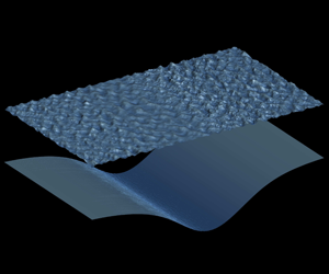
Figure 2. (a) Direct observation of the surface signature, denoted by the instantaneous surface wave elevation field. (b) Temporal evolution of the steepness ratio. In (a), also shown are the interface elevation and the boundaries of the regions used for spectral analysis in § 3.3, denoted by dashed lines. For clarity, we only plot part of the computational domain. The internal wave propagates in the  $+x$ direction. In (b), two trendlines are plotted.
The surface signature can be directly observed from the surface elevation with the naked eye (Woodson Reference Woodson2018). In our simulation, the initial surface wave field is statistically homogeneous and the surface signature is found to form gradually and maintain throughout the simulation. We present an example of the instantaneous surface elevation and the interface elevation in figure 2(a). As shown, a rough surface region with increased wave steepness is formed above the leading edge of the internal wave (figure 1). Right behind the rough region there is a smooth region where the surface wave steepness is significantly reduced. The rough and smooth regions correspond to a pair of bright and dark bands on satellite images. Qualitatively, the surface signature observed in the present study shows several key features in remote sensing observations, including the location of the rough and smooth regions with respect to the internal wave, their length scales and the propagating speed. For the purpose of quantitative comparison with observational data, the wave-phase-resolved surface signature can potentially be valuable by providing hydrodynamic information to radar electromagnetic signal simulations (e.g. Liu & He Reference Liu and He2016; Yoshida Reference Yoshida2017), which were conducted on artificially generated ocean surfaces in the literature.
The formation of the surface signature is a transient process, during which the initially homogeneous surface waves respond to the time-varying surface strain field driven by the internal wave. To illustrate this process, we define the density ratio  $R_{S}=\int \!S_{rough}\,\text{d}x\,\text{d}y/\int \!S_{smooth}\,\text{d}x\,\text{d}y$, where
  $S(x,y)=[(\unicode[STIX]{x2202}\unicode[STIX]{x1D702}_{u}/\unicode[STIX]{x2202}x)^{2}+(\unicode[STIX]{x2202}\unicode[STIX]{x1D702}_{u}/\unicode[STIX]{x2202}y)^{2}]^{1/2}$ is the local steepness and the integrations are performed in the regions denoted by the dashed lines in figure 2(a). As shown in figure 2(b),
  $R_{S}$ first undergoes a transient, linear growth stage (dashed line) and then settles around
  $2.1$ (dotted line). The time scale of the transient process is approximately
  $7.7T_{p}$, which is much shorter than the time scale of the internal wave:
  $l_{iw}/c_{iw}=117T_{p}$. Therefore, for a fixed point in the Eulerian frame, we expect the surface wave energy to undergo a rapid transient process as the time-varying surface strain field driven by the internal solitary wave as it passes by.
3.2 Quantitative analysis of surface signature
To quantify the roughness change, we calculate the local steepness (figure 3a) and find that the wave steepness in the rough region is higher than that in the smooth region in a statistical sense. As shown in figure 3(b), the surface wave energy change  $\unicode[STIX]{x0394}E/E_{0}$ calculated from the wavenumber spectrum can also reveal the surface signature pattern. We divide the computational domain into 48 regions along the
  $x$ direction, each with a size of
  $10.4~\text{m}\times 125~\text{m}$. Then we conduct a two-dimensional Fourier transform on the product of the surface elevation
  $\unicode[STIX]{x1D702}_{u}(x,y)$ and a window function in each region and obtain the wavenumber spectrum
  $E(k_{x},k_{y})$. Considering that the surface wave field should be statistically homogeneous in the
  $y$ direction, we perform averaging to obtain the one-dimensional wavenumber spectrum
  $E(k_{x})=\int E(k_{x},k_{y})\,\text{d}k_{y}$.

Figure 3. Quantitative analysis of the surface signature. (a) Plan view of the instantaneous local steepness  $S=[(\unicode[STIX]{x2202}\unicode[STIX]{x1D702}_{u}/\unicode[STIX]{x2202}x)^{2}+(\unicode[STIX]{x2202}\unicode[STIX]{x1D702}_{u}/\unicode[STIX]{x2202}y)^{2}]^{1/2}$ of the surface wave field, where
  $\unicode[STIX]{x1D702}_{u}$ is the surface elevation. (b) The change in surface wave energy
  $\unicode[STIX]{x0394}E$ normalized by the unperturbed value
  $E_{0}$, where the black solid line denotes the mean value over all wavenumbers and the error bar denotes the standard deviation. The shaded area in light blue denotes the range of the empirical estimation (Alpers Reference Alpers1985). (c) Surface current induced by the internal wave. Our numerical result is denoted by the blue solid line and the first-order approximation is denoted by the black dashed line.
To clarify the correlation between the wave energy change and the surface motion induced by the internal wave, we provide another estimation according to the formula proposed by Alpers (Reference Alpers1985):  $\unicode[STIX]{x0394}E/E_{0}=-\unicode[STIX]{x1D70F}\,\text{d}U/\text{d}x$, where
  $\unicode[STIX]{x1D70F}=21.2{-}212~\text{s}$ is a relaxation time set empirically based on the time scale of the surface wave energy transfer processes including wind input, nonlinear interaction and dissipation and
  $\text{d}U/\text{d}x$ is the gradient of the surface current. Overall, the results are consistent and show the same trend in the wave energy change, which sees an apparent correlation with the current gradient (figure 3b). Here the surface current is calculated by performing averaging in the spanwise direction and time averaging in the reference frame moving with the internal wave. The gradient of the current
  $\text{d}U/\text{d}x$ is then calculated from
  $U(x)$. Instead of direct calculation with a finite difference approximation, we compute
  $\text{d}U/\text{d}x$ by minimizing a functional to avoid extreme values caused by irregularity and noise in
  $U(x)$ (Chartrand Reference Chartrand2011). The first-order approximation of the current can also be estimated from mass conservation:
  $-c_{iw}\unicode[STIX]{x1D702}_{l}/(h_{u}-\unicode[STIX]{x1D702}_{l})$. Overall, the two results agree with each other except for small deviations in the region above the internal wave trough (figure 3c).
3.3 Surface waves in the wavenumber–frequency domain
To elucidate the formation of the surface signature, we conduct spectral analysis on the surface elevation in the frame of reference travelling with the internal wave. The data are extracted from two domains above the internal wave trough, one in the smooth region and the other in the rough region (see the dashed lines in figure 2a). The size of each subdomain is  $21~\text{m}\times 125~\text{m}$, smaller than the actual length scale of the smooth and rough regions to ensure the homogeneity requirement in Fourier analysis. The wavenumber–frequency spectrum
  $E(k_{x},k_{y},\unicode[STIX]{x1D714})$ of surface elevation is then calculated in each subdomain. To better reveal the roughness change of the surface wave field, we further calculate the slope spectrum
  ${\mathcal{S}}(k_{x},k_{y},\unicode[STIX]{x1D714})=(k_{x}^{2}+k_{y}^{2})E$. In the following analysis, the integrated spectrum
  ${\mathcal{S}}(k_{x},\unicode[STIX]{x1D714})=\int {\mathcal{S}}(k_{x},k_{y},\unicode[STIX]{x1D714})\,\text{d}k_{y}$ is presented for clarity. In terms of the physical meaning, the slope spectrum
  ${\mathcal{S}}(k_{x},k_{y},\unicode[STIX]{x1D714})$ can be seen as the spectral space counterpart to the steepness function
  $S(x,y)$ in figure 3(a).

Figure 4. Wavenumber–frequency slope spectrum of surface waves in the (a) smooth region and (b) rough region. The spectrum is normalized by the maximum value  ${\mathcal{S}}_{m}$. The dashed curves denote the dispersion relation of the surface waves in the moving frame of reference:
  $\unicode[STIX]{x1D714}=(U_{m}-c_{iw})k_{x}+\sqrt{g|k_{x}|}$, where
  $U_{m}$ is the maximum value of the surface current
  $U$ (see figure 3). The white cross denotes the maximum frequency of the right-moving surface wave
  $\unicode[STIX]{x1D714}_{m}=-g/4(U_{m}-c_{iw})$. The black filled circle denotes the peak surface wave. The asymmetric behaviours of the surface waves mostly occur in zones I and II.
From the contours of the wavenumber–frequency spectra (figure 4), we can separately identify the energy associated with the two different eigenfunctions in the internal wave system: the baroclinic mode energy is located in the low-frequency portion, while the barotropic mode energy is primarily along the dispersion relation curve of the surface wave in the moving frame of reference as shown by the dashed lines. Because of the space and time limits of the domain used for Fourier analysis, the wave components of low frequency, e.g.  $\unicode[STIX]{x1D714}/\sqrt{g/h_{u}}\sim O(3)$, appear as white-noise-like bands on the spectrum. In the moving frame, the surface motion induced by the internal wave is a countercurrent because
  $U-c_{iw}<0$. As a result, there exists a maximum frequency
  $\unicode[STIX]{x1D714}_{m}=-g/4(U_{m}-c_{iw})$ for surface waves propagating against the current (Donato et al. Reference Donato, Peregrine and Stocker1999; Nardin et al. Reference Nardin, Rousseaux and Coullet2009).
The surface signature can be identified from the asymmetric behaviours of the surface waves. In the rough region, we observe a distinct difference in both right-moving and left-moving surface waves (see zones I and II in figure 4b) compared with those in the smooth region (figure 4a). Let  $\unicode[STIX]{x1D6FF}S$ (respectively,
  $\unicode[STIX]{x1D6FF}E$) denote the difference of the slope (respectively, energy) spectrum between the rough and smooth region and we have
  $\unicode[STIX]{x1D6FF}S=k^{2}\unicode[STIX]{x1D6FF}E$. The wave energy change in zone I is larger than that in zone II, i.e.
  $\unicode[STIX]{x1D6FF}E_{I}>\unicode[STIX]{x1D6FF}E_{II}$, because the background surface wave energy is maximal near the peak wave component (see the black filled circle in figure 4). Meanwhile, the wavenumber of wave components in zone II, especially those shorter than
  $O(1~\text{m})$, or
  $k_{x}h_{u}<O(50)$, is higher than that in zone I, namely,
  $k_{I}<k_{II}$. Overall, the contribution of the zone II waves to the roughness change is comparable to that of zone I waves, i.e.
  $\unicode[STIX]{x1D6FF}S_{II}\sim \unicode[STIX]{x1D6FF}S_{I}$.
The asymmetric behaviours of the right-moving surface waves in zone I, such as the increased magnitude towards the leading edge of the internal wave, are consistent with previous studies (Bakhanov & Ostrovsky Reference Bakhanov and Ostrovsky2002; Kodaira et al. Reference Kodaira, Waseda, Miyata and Choi2016; Jiang et al. Reference Jiang, Kovačič, Zhou and Cai2019). In contrast, there are no previous studies reporting the contribution of the left-moving surface waves of small length scales in zone II, because short surface wave dynamics were usually neglected. For example, Jiang et al. (Reference Jiang, Kovačič, Zhou and Cai2019) studied surface waves yielding the long-wave (shallow-water) approximation, which assumes that the surface wavelength scales are much greater than the fluid layer thickness. Even for the peak surface waves  $k_{x}h_{u}\approx 4.4$, the upper layer fluid can still be viewed as deep water (e.g. Dean & Dalrymple Reference Dean and Dalrymple1991).
4 Conclusions
In this study, we have performed the first simulation to directly capture the surface roughness signature induced by an internal wave using a deterministic phase-resolved two-layer fluid model. A realistic setting for the interaction between a broadband surface wave field and a typical oceanic internal wave is considered. The wave dynamics of nearly  $4.2\times 10^{6}$ independent components are resolved, covering the wide range of length scales between the internal wave and short surface waves.
Our results show that the formation of the surface signature is essentially an energy-conservative process. In other words, energy sources and sinks, including wind input and wave breaking, are not necessarily the direct cause of the surface signature. With the surface wave and internal wave dynamics captured, the surface signature is quantified using the wave geometry and the energy change. For the first time, the roughness change is identified on the full wavenumber–frequency slope spectrum in a realistic ocean setting of internal and surface waves, which substantiates the contribution of the asymmetric behaviours of the right-moving surface waves to the roughness change. Moreover, our result shows that left-moving waves shorter than  $O(1~\text{m})$ also play an important role in the surface signature formation.
Admittedly, we have neglected the effects of the stratification associated with the continuous density profile, turbulence and the stronger nonlinearity in internal waves. For example, the internal wave amplitude in the present computational case is smaller than that in the original field observation (Stanton & Ostrovsky Reference Stanton and Ostrovsky1998). Consequently, the magnitude of the surface current induced by the internal wave and thus the roughness change may be underestimated. In future study, the stratification effects can also be captured by solving the full three-dimensional Navier–Stokes equations, yet at a considerably high computational cost not affordable with the current computing power.
Acknowledgements
The authors gratefully acknowledge the referees for their constructive and valuable comments. This work is supported by the Office of Naval Research.
Declaration of interests
The authors report no conflict of interest.
Supplementary material and movies
Supplementary material and movies are available at https://doi.org/10.1017/jfm.2020.200.


