2.1. Initialisation

The problem consists in extending the analysis conducted at $M_c=1.1$ in Vadrot, Aurélien & Alexis (Reference Vadrot, Giauque and Corre2020) by performing a DNS of a three-dimensional mixing layer at a convective Mach number $M_c=2.2$ for air considered as a PG and for a BZT DG: the perfluorotripentylamine (FC-70, $C_{15}F_{33}N$). Physical parameters associated with FC-70 and used in these DNS are given in table 1.

Table 1. Physical parameters of FC-70 (Cramer Reference Cramer1989). The critical pressure $p_c$, the critical temperature $T_c$, the boiling temperature $T_b$ and the compressibility factor $Z_c=p_c v_c/(RT_c)$ are the input data for the Martin–Hou equation. The critical specific volume $v_c$ is deduced from the aforementioned parameters. The exponent $n$ and the $c_v(T_c)/R$ ratio are used to compute the heat capacity $c_v(T)$ ($R=\mathcal {R}/M$ being the specific gas constant computed from the universal gas constant $\mathcal {R}$ and $M$, the gas molar mass).

The initial thermodynamic state is chosen inside the inversion region in order to favour the occurrence of expansion shocklets, physically allowed in BZT DGs. Figure 1 shows the initial state in the $p$–$v$ diagram and its distribution during the beginning of the self-similar regime at $\tau =4000$ for DG flow. The initial value of the fundamental derivative is $\varGamma _{\textit {initial}} = -0.284$ which makes possible the appearance of expansion shocklets. The distribution spreads inside and slightly outside the inversion region. One can also note that the distribution does not perfectly follow the initial adiabatic curve. Mechanical dissipation and shocklets entropy losses are responsible for this discrepancy because their effect cannot be neglected at $M_c=2.2$.

For air, the same values of reduced specific volume and reduced pressure are selected for the initial thermodynamic state. Critical values used for air are the critical pressure $p_c=3.7663 \times 10^6$ Pa and the specific volume $v_c=3.13 \times 10^{-3}$ m$^3$ kg$^{-1}$ (Stephan & Laesecke Reference Stephan and Laesecke1985).

Key non-dimensional parameters are the convective Mach number (1.3) and the Reynolds number based on the initial momentum thickness $\delta _{\theta ,0}$

(2.1)\begin{equation} Re_{\delta_{\theta,0}}=\Delta u \delta_{\theta,0}/\nu, \end{equation}

where $\nu$ denotes the kinematic viscosity and the momentum thickness at time $t$ is defined as

(2.2)\begin{equation} \delta_\theta(t) = \frac{1}{\rho_{0} (\Delta u)^{2}} \int_{-\infty}^{+\infty} \bar{\rho} \left( \frac{(\Delta u)^{2}}{4}-{\tilde{u}}_{x}^{2} \right) {\textrm{d} y}, \end{equation}

with $\rho _{0} = (\rho _{1} + \rho _{2})/2$ the averaged density and $\tilde {u}_x$ the Favre-averaged streamwise velocity defined in (2.9).

The initial momentum thickness Reynolds number is set equal to $160$ for all the DNS following Pantano & Sarkar (Reference Pantano and Sarkar2002). Table 2 summarises the computational parameters of simulations performed for different $M_c$ (domain size, number of grid elements, dimensional values of velocity, initial momentum thickness and initial turbulent structures sizes). Additional DG simulations given in Appendix A have been performed for other domain sizes and resolutions to validate the current DNS. The impact on the selection of the self-similar period is also analysed in Appendix A.

Table 2. Simulation parameters. $L_x$, $L_y$ and $L_z$ denote computational domain lengths measured in terms of initial momentum thickness; $N_x$, $N_y$ and $N_z$ denote the number of grid points; $L_0$ denotes the size of initial turbulent structures ($k_0=2{\rm \pi} /L_0$) measured in terms of initial momentum thickness. All grids are uniform.

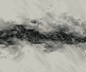
The temporal mixing layer consists of two streams flowing in opposite directions. The velocity in the upper part of the domain $U_1$ is set equal to $-\Delta u/2$, whereas $U_2$ is set to $\Delta u/2$. A representation of the computational domain is provided in figure 2. A snapshot of the velocity magnitude is also plotted for the DG DNS at $M_c=2.2$. A further analysis of the flow field visualisation is given in Appendix B. Periodic boundary conditions are imposed in the $x$ and $z$ directions and non-reflective conditions are set in the $y$ directions using the Navier–Stokes characteristic boundary conditions model proposed by Poinsot & Lele (Reference Poinsot and Lele1992).

Figure 2. Configuration of the temporal mixing layer. The velocity magnitude is plotted for the DG DNS at $M_c=2.2$ at $\tau = 4000$.

The streamwise velocity field is initialised using an hyperbolic tangent profile

(2.3)\begin{equation} \bar{u}_{x}(y) = \frac{\Delta u}{2} \tanh{\left(-\frac{y}{2\delta_{\theta, 0}}\right)}. \end{equation}

The complete streamwise velocity field is obtained by adding fluctuations to the average velocity. For the $y$ and $z$ components, the average velocity is set equal to zero. A Passot–Pouquet spectrum is imposed for initial velocity fluctuations

(2.4)\begin{equation} E(k) = (k/k_0)^4 \exp({-}2(k/k_0)^2), \end{equation}

where $k$ denotes the wavenumber. The peak wavenumber $k_0$ controls the size of the initial turbulent structures. Its influence on the mixing layer growth is investigated in Appendix A. Its value only influences the initial unstable growth regime. It has been noted that a larger value of $k_0$ accelerates the transition to the unstable growth. Its value for each DNS is given in table 2. The velocity field is then filtered to initialise turbulence only inside the initial momentum thickness.

2.2. Governing equations

In order to describe the temporally evolving mixing layer, the unsteady, three-dimensional, compressible Navier–Stokes equations are solved:

(2.5)$$\begin{gather} \frac{\partial \rho}{\partial t} + \frac{\partial (\rho u_{i})}{\partial x_{i}}=0, \end{gather}$$

(2.6)$$\begin{gather}\frac{\partial (\rho u_{i})}{\partial t}+ \frac{\partial (\rho u_{i} u_{j})}{\partial x_{j}} ={-}\frac{\partial p}{\partial x_{i}} + \frac{\partial \tau_{ij}}{\partial x_{j}}, \end{gather}$$

(2.7)$$\begin{gather}\frac{\partial (\rho E)}{\partial t}+\frac{\partial [(\rho E+p)u_{j}]}{\partial x_{j}} = \frac{\partial ( \tau_{ij} u_{i}-q_{j})}{\partial x_{j}}, \end{gather}$$

where $\tau _{ij} = \mu ({\partial u_{i}}/{\partial x_{j}}+ {\partial u_{j}}/{\partial x_{i}} -\frac {2}{3}({\partial u_{k}}/{\partial x_{k}})\delta _{ij})$ denotes the viscous stress tensor ($\mu$ the dynamic viscosity), $E = e + \frac {1}{2} u_{i}u_i$, the specific total energy ($e$, the specific internal energy), $q_{j} = - \lambda ({\partial T}/{\partial x_j})$, the heat flux given by Fourier's law ($\lambda$, the thermal conductivity).

Part of this study is conducted thanks to the analysis of the turbulent kinetic energy (TKE) equation terms. It requires to decompose density, pressure and velocity into mean and fluctuating components as follows:

(2.8)\begin{equation} \left\{ \begin{array}{@{}l} \rho = \bar{\rho} + \rho',\\ p = \bar{p} + p', \\ u_{i} = \tilde{u}_{i} + u_{i}'', \end{array}\right. \end{equation}

where $\bar {\phi }$ denotes the Reynolds average for a flow variable $\phi$ while the Favre average $\tilde {\phi }$ is defined as

(2.9)\begin{equation} \tilde{\phi} = \frac{\overline{\rho \phi}}{\bar{\rho}}. \end{equation}

Reynolds fluctuations are noted $\phi '$ while Favre fluctuations are noted $\phi ''$. Reynolds averaging is equivalent to plane averaging along the $x$ and $z$ directions because of the use of periodic boundary conditions. The TKE equation is obtained from the Navier–Stokes equation by applying the averaging process

(2.10)\begin{align} \frac{\partial \bar{\rho} \tilde{k}}{\partial t}+\frac{\partial \bar{\rho} \tilde{k} \tilde{u}_{j}}{\partial x_{j}}& = \underbrace{-\overline{\rho u_{i}'' u_{j}''}\frac{\partial \tilde{u}_{i}}{\partial x_{j}}}_{\textit{Production}} -\underbrace{\overline{\tau_{ij}' \frac{\partial u_{i}''}{\partial x_{j}}}}_{\textit{Dissipation}} \nonumber\\ &\quad -\underbrace{\frac{1}{2}\frac{\partial \overline{\rho u_{i}'' u_{i}'' u_{j}''}}{\partial x_{j}}}_{\textit{Turbulent}\ \textit{transport}} - \underbrace{\frac{\partial \overline{p' u_{i}''}}{\partial x_i}}_{\textit{Pressure}\ \textit{transport}}+\underbrace{\frac{\partial \overline{u_{i}''\tau_{ij}'}}{\partial x_j}}_{\textit{Viscous}\ \textit{transport}} \nonumber\\ &\quad +\underbrace{\overline{p' \frac{\partial u_{i}''}{\partial x_i}}}_{\textit{Pressure}\ \textit{dilatation}} -\underbrace{\overline{u_{i}''} \left(\frac{\partial \bar{p}}{\partial x_i}-\frac{\partial \bar{\tau}_{ij}}{\partial x_j}\right)}_{\textit{Mass-flux}\ \textit{term}}, \end{align}

where $\tilde {k} = \frac {1}{2} \widetilde {u_{i}''u_{i}''}$ denotes the specific TKE. The main terms of (2.10) are production, dissipation and transport terms. Pressure dilatation and mass-flux terms (the later comprises the baropycnal work) are equal to zero in the incompressible case. The dissipation term can be decomposed into a solenoidal, a low Reynolds number and a dilatational component. The latter is associated with losses occurring in eddy shocklets. Lee, Lele & Moin (Reference Lee, Lele and Moin1991) expressed the dilatational dissipation also called the compressible dissipation as

(2.11)\begin{equation} \epsilon_d ={-}\frac{4}{3} \overline{\nu\left(\frac{\partial u_k''}{\partial x_k}\right)^2} - 2 \overline{u_k'' \frac{\partial \nu'}{\partial x_k} \frac{\partial u_k''}{\partial x_k}}. \end{equation}

This expression comprises the effect of viscosity variations, unlike Sarkar & Lakshmanan (Reference Sarkar and Lakshmanan1991) and Zeman (Reference Zeman1990), who expressed it as $\epsilon _d=-\frac {4}{3} \bar {\nu }\overline {({\partial u_k''}/{\partial x_k})^2}$, neglecting viscosity variations. For decaying compressible turbulence, Lee et al. (Reference Lee, Lele and Moin1991) found that the Sarkar & Lakshmanan (Reference Sarkar and Lakshmanan1991) and Zeman (Reference Zeman1990) expression overestimates by approximately $15\,\%$ the compressible dissipation.

In addition to (2.5), (2.6) and (2.7), the thermal PG and the following calorific EoSs are used for air:

(2.12)\begin{equation} \left\{\begin{array}{@{}l} p=\rho R T ,\\ e=e_{\textit{ref}}+\displaystyle\int^T_{T_{\textit{ref}}} c_v(T') \,\textrm{d}T', \end{array}\right. \end{equation}

where $R$ is the specific gas constant, $c_v$ the specific heat capacity, $p$ the pressure, $T$ the temperature, $\rho$ the density.

For FC-70, the Martin–Hou EoS (referred to as MH) will be retained to provide an accurate representation of BZT DG thermodynamic behaviour (Guardone, Vigevano & Argrow Reference Guardone, Vigevano and Argrow2004)

(2.13)\begin{equation} \left\{\begin{array}{@{}l} p = \displaystyle\dfrac{RT}{v-b}+\sum_{i=2}^{5} \dfrac{A_i+B_iT+C_i\ \textrm{e}^{{-}kT/T_c}}{(v-b)^i}, \\ e = e_{\textit{ref}} + \displaystyle\int_{T_{\textit{ref}}}^{T} c_v(T') \,\textrm{d}T' + \sum_{i=2}^{5} \dfrac{A_i+C_i (1+kT/T_c) \ \textrm{e}^{{-}kT/T_c}}{(i-1)(v-b)^{i-1}}, \end{array}\right. \end{equation}

where $(\cdot )_{\textit {ref}}$ denotes a reference state, $b=v_c(1-(-31\,883Z_c+20.533)/15)$, $k=5.475$ and the coefficients $A_i$, $B_i$ and $C_i$ are numerical constants determined by Martin & Hou (Reference Martin and Hou1955) and Martin, Kapoor & De Nevers (Reference Martin, Kapoor and De Nevers1959) from physical parameters summarised in table 1.

To complete the thermodynamic description of the BZT DG, Chung's model is used to compute dynamic viscosity and thermal conductivity (Chung et al. Reference Chung, Ajlan, Lee and Starling1988). FC-70 is assumed to behave as a non-polar gas, its dipole moment is therefore neglected (Shuely Reference Shuely1996). For PG transport coefficients, Sutherland's model is used associated with a constant Prandtl number set equal to $0.71$. Values of the initial Prandtl number are given in Appendix C for DG flows. The selected constants for Sutherland's law are the ones given by White (Reference White1998).

2.3. Numerical set-up

DNS are performed using the explicit and unstructured numerical solver AVBP. It solves the three-dimensional unsteady compressible Navier–Stokes equations coupled with the PG EoS (2.12) for air and the MH EoS for FC-70 (2.13) using a two-step time-explicit Taylor Galerkin scheme for the hyperbolic terms based on a cell vertex formulation (Colin & Rudgyard Reference Colin and Rudgyard2000). The scheme provides high spectral resolution and low numerical dissipation ensuring a third-order accuracy in space and in time. AVBP is designed for massively parallel computation and can be used to perform LES as well as DNS simulations (Desoutter et al. Reference Desoutter, Habchi, Cuenot and Poinsot2009; Cadieux et al. Reference Cadieux, Domaradzki, Sayadi, Bose and Duchaine2012). The scheme is completed with a shock capturing method. In regions where strong gradients exist, an additional dissipation term is added following the approach of Cook & Cabot (Reference Cook and Cabot2004). Its impact on the resolution of the smallest scales has been analysed in a previous article (Giauque et al. Reference Giauque, Corre and Vadrot2020).

3.1. Temporal evolution and self-similarity

Figure 3 shows the temporal evolution of the momentum thickness normalised by its initial value. This key quantity characterises the development of mixing layers. Time is non-dimensional ($\tau =t\Delta u/\delta _{\theta ,0}$). The evolution is plotted for three different convective Mach numbers ($M_c=0.1/1.1/2.2$). Results at $M_c=1.1$ are extracted from Vadrot, Aurélien & Alexis (Reference Vadrot, Giauque and Corre2020). The same Reynolds number ($Re_{\delta _{\theta ,0}}=160$) based on the initial momentum thickness is used for the three different DNS. Simulation parameters are given in table 2. At $M_c=2.2$, the size of initial turbulent structures has been enlarged in order to speed up the development of the mixing layer.

Figure 3. Temporal evolution of the mixing layer momentum thickness for $M_c=0.1/1.1/2.2$ using air with PG EoS. Slopes are non-dimensional and standard deviations computed over the self-similar period are indicated on the plot.

One can identify three main phases: an initial delay caused by a transition of modes from the modes in which TKE is initially injected to the most unstable ones; an unstable over-linear growth; and the self-similar period, during which the mixing layer evolves linearly with time. The procedure used to select the self-similar period is detailed in subsequent paragraphs.

At $M_c=2.2$, one can notice that the mixing layer takes a much longer time to develop. This is consistent with observations of Pantano & Sarkar (Reference Pantano and Sarkar2002) who noticed that the time necessarily to reach self-similar regime increases with compressibility. Self-similarity is reached around $\tau \approx 11\,500$ after a long unstable growth phase. As a comparison, at $M_c=0.1$ and $M_c=1.1$, self-similarity is reached respectively at $\tau =700$ and $\tau =1700$. Moreover, the self-similar period is also stretched as the convective Mach number increases.

A long time delay is observed at the beginning of the simulation. That delay is associated with the transition of modes. TKE is initially injected at a given integral length set equal to $L_x/8$. Afterwards, energy is distributed over the whole spectrum and some unstable modes are amplified, leading to the unstable growth phase. In order to reduce this time delay, initial turbulent structures have been chosen to be larger in proportion to the initial momentum thickness at $M_c = 2.2$ when compared to other convective Mach numbers (table 2). This modification of initial turbulent structures size does not impact the growth rate over the self-similar regime. This has been carefully verified for DG flows in Appendix A.

In addition, domain lengths are doubled in the $x$ and $z$ directions and multiplied by four in the $y$ direction when compared with DNS at $M_c=1.1$, relative to initial momentum thicknesses. This enables the mixing layer to develop until larger values of $\delta _{\theta }(t)/\delta _{\theta ,0}$ and to obtain a long enough self-similar period without reaching the domain boundaries. Other simulations performed with smaller domains did not allow the flow to reach self-similarity.

Slopes and standard deviations mentioned in figure 3 are computed over the self-similar period. One can observe that the growth rate is divided by a factor of approximately two between DNS at $M_c=2.2$ and at $M_c=1.1$. Indeed, compressibility effects tend to reduce mixing layer development as the convective Mach number increases.

DNS performed at $M_c=0.1$ constitutes our reference incompressible case used to plot $\dot {\delta }_\theta /\dot {\delta }_{\theta ,inc}=f(M_c)$. The computed growth rate is approximately $0.0131$ which is relatively close to the empirical value of $0.016$ given by Pantano & Sarkar (Reference Pantano and Sarkar2002). One can notice a very short unstable growth phase when compared with larger convective Mach number cases.

Self-similarity is a major characteristic of mixing layers: during the self-similar period, flow development can be described using single length and velocity scales. The momentum thickness linearly evolves with time. This particular state in the development of mixing layers is widely used to extract key features of mixing layers. The well-known chart giving the evolution of the mixing layer growth rate as a function of the convective Mach number (Papamoschou & Roshko Reference Papamoschou and Roshko1988) is plotted during the self-similar regime. This period is also used to investigate the balance of the TKE equation, because temporal solutions can be averaged during self-similarity since the flow is in a statistically stable state.

The selection of the self-similar period is thus a key point in the study of turbulent mixing layers, but this choice is difficult, especially at high compressible regimes which require lengthy simulations. One can note that, in our case, the time required to achieve self-similarity is multiplied by a factor of approximately five when the convective Mach number increases from $M_c=1.1$ to $M_c=2.2$.

Lots of authors evoke difficulties in reaching self-similarity (Pantano & Sarkar Reference Pantano and Sarkar2002; Pirozzoli et al. Reference Pirozzoli, Bernardini, Marié and Grasso2015) particularly because of computational domain lengths. Moreover, criteria to define self-similarity are not standardised. Superposition of the mean velocity profiles, linear evolution of the momentum thickness, collapse of the Reynolds stress profiles are three different ways to define the self-similar period.

The same methodology used in Vadrot, Aurélien & Alexis (Reference Vadrot, Giauque and Corre2020) is applied here to select the self-similar period: it relies on the stabilisation of the streamwise production term integrated over the whole domain. The underlying reason for using this criterion comes from Vreman et al. (Reference Vreman, Sandham and Luo1996), who demonstrated the following relation between the mixing layer growth rate and the production power ($\bar {\rho } P_{xx} = - \overline {\rho u_x''u_y''}({\partial \tilde {u}_x}/{\partial y})$):

(3.1)\begin{equation} \delta_{\theta}'=\frac{\textrm{d}\delta_\theta}{\textrm{d}t}=\frac{2}{\rho_0 (\Delta u)^2} \int \bar{\rho} P_{xx} \,{\textrm{d} y}. \end{equation}

Figure 4 shows the temporal evolution of the non-dimensional streamwise production integrated over the whole domain for the three DNS at $M_c$ ranging from $0.1$ to $2.2$ performed for air using the PG EoS. A constant integrated production is directly related to a self-similar regime according to (3.1). Selected self-similar periods are indicated on each plot. As the convective Mach number increases, the maximum peak of integrated turbulent production decreases, which is consistent with the decrease of the momentum thickness growth rate. Time required to achieve self-similarity lengthens but self-similar periods last longer.

Figure 4. Temporal evolution of the non-dimensional streamwise turbulent production term integrated over the whole domain $P_{int}^*= (1/(\rho _0(\Delta u)^3 )) \int _{L_y} \bar {\rho } P_{xx} \,{\textrm {d} y}$ (with $\bar {\rho } P_{xx}(y) = - \overline {\rho u_x''u_y''}({\partial \tilde {u}_x}/{\partial y})$) at $M_c=0.1$ (a), $M_c=1.1$ (b) and $M_c=2.2$ (c). Results are shown for the air using PG EoS. Selections of self-similar period are indicated on each plot.

Difficulties can be encountered in obtaining a fully stable plateau with an almost constant integrated turbulent production. Domain lengths have a major influence on self-similarity. The evolution of the turbulent production follows a piecewise decrease, reaching several plateaus. It is observed that these piecewise plateaus are directly related to integral lengths scales. When some turbulent structures grow and become too large for the computational domain, the integrated turbulent production decreases and reaches another plateau lower than the previous one. The mixing layer therefore adapts its growth to domain lengths when the computational box is not large enough. Since the integrated turbulent production is related to the mixing layer growth rate, a lower plateau leads to a smaller mixing layer growth rate. Great care therefore needs to be taken when selecting the size of the computational domain, and a good stabilization of the integrated turbulent production must be reached in order to precisely select the self-similar period. Influence of the domain size on self-similarity is thoroughly investigated in Appendix A for DG flows and correlations with integral length scales are analysed.

3.2. Validation over the self-similar period

Since self-similar periods are now well defined for each DNS, it is possible to plot the evolution of the mixing layer growth rate with respect to the convective Mach number. Figure 5 shows a comparison between current PG results and available numerical (Freund, Lele & Moin Reference Freund, Lele and Moin2000; Kourta & Sauvage Reference Kourta and Sauvage2002; Pantano & Sarkar Reference Pantano and Sarkar2002; Fu & Li Reference Fu and Li2006; Zhou, He & Shen Reference Zhou, He and Shen2012; Martínez Ferrer, Lehnasch & Mura Reference Martínez Ferrer, Lehnasch and Mura2017; Matsuno & Lele Reference Matsuno and Lele2020) and experimental results (Rossmann et al. Reference Rossmann, Mungal and Hanson2001) from the literature. Current DNS follow the tendency observed and described in the literature: the well-known compressibility-related reduction of the momentum thickness growth rate as $M_c$ increases. From the incompressible case to $M_c=2.2$, the mixing layer growth rate is divided by a factor of approximately five. Standard deviations have also been computed and are reported on the plot. It represents approximately 5 % of the computed growth rates. It is rather difficult to reduce this uncertainty because of difficulties encountered in reaching perfect self-similarity. This is also illustrated by the scattering of literature results, which might be a consequence of this phenomenon. Moreover, the lack of numerical results at highly compressible regimes makes the validation process more complex.

Figure 5. Evolution of the mixing layer growth rate with respect to the convective Mach number for air using PG EoS. Comparison is made with available DNS results in literature and experimental results by Rossmann et al. (Reference Rossmann, Mungal and Hanson2001). Standard deviations are indicated on the plot.

Yet, numerical parameters given in table 3 confirm the validation of the current DNS. The integral lengths $l_x$ and $l_z$ are computed using the streamwise velocity field:

(3.2)$$\begin{gather} l_x =\frac{1}{2\overline{{u_x'}^2}} \int_{{-}L_x/2}^{L_x/2} \overline{{u_x'}(\boldsymbol{x}){u_x'}(\boldsymbol{x}+r\boldsymbol{e}_{\boldsymbol{x}})}\,\textrm{d}r, \end{gather}$$

(3.3)$$\begin{gather}l_z =\frac{1}{2\overline{{u_x'}^2}} \int_{{-}L_z/2}^{L_z/2} \overline{{u_x'}(\boldsymbol{x}){u_x'}(\boldsymbol{x}+r\boldsymbol{e}_{\boldsymbol{z}})}\,\textrm{d}r. \end{gather}$$

Table 3. Non-dimensional parameters computed at the beginning and at the end of the self-similar period for $M_c=2.2$ simulations; $Re_{\lambda _x}$ denotes the Reynolds number based on the longitudinal Taylor microscale $\lambda _x=\sqrt {2\overline {{u'}^{2}_{x}}/\overline {(\partial {u_x'}/\partial x)^2}}$ computed at the centreline; $L_\eta$ denotes the Kolmogorov length scale computed at the centreline.

Integral length scales show that the domain is chosen sufficiently large. The largest value $0.20$ is obtained at the end of the self-similar period for DG flow at $M_c=1.1$. Otherwise, values do not exceed $0.16$ in the streamwise direction and $0.13$ in the $z$ direction. As a comparison, the Pantano & Sarkar (Reference Pantano and Sarkar2002) integral length scale reaches $0.178$ in the streamwise direction for a configuration with $M_c=0.7$ and a density ratio of $4$. Appendix A also confirms that domain lengths have been properly chosen for DG mixing layer at $M_c=2.2$.

The ratio $r=L_\eta /\Delta x$ characterises the resolution of simulations. The larger the ratio, the better the resolution. Minimum value is approximately $0.52$ computed for DNS at $M_c=2.2$. For other simulations, values are larger than $0.6$ and the maximum value is $1.64$ for PG at $M_c=2.2$ because of small dissipation in high compressible regimes. As a comparison, the Pantano & Sarkar (Reference Pantano and Sarkar2002) ratio is approximately $0.38$ for the most resolved simulation and recently Matsuno & Lele (Reference Matsuno and Lele2020) performed a DNS at $M_c=2.0$ with a $L_\eta /{\textrm {d} x}$ ratio equal to $0.41$. One can thus consider that turbulent scales are adequately resolved for all simulations presented in this paper since in addition the TKE is very low close to the Kolmogorov scale (Moin & Mahesh Reference Moin and Mahesh1998).

4.1. Temporal evolution

As previously done for the PG mixing layer, it is required to precisely define the self-similar range for the DG flow. This is done through both figures 6 and 7. Figure 6 enables the comparison of normalised DG momentum thickness over time at three different convective Mach numbers: $M_c=0.1-1.1-2.2$. The three DNS are performed at the same initial Reynolds number $Re_{\delta _{\theta ,0}}=160$. Additional simulation parameters are given in table 2. At $M_c=0.1$, similarly to the PG mixing layer, the domain length is doubled in the $y$ direction to get a long enough self-similar period. At $M_c=2.2$, the domain length is divided by two in the $y$ direction when compared with PG flow. The domain is therefore large enough to reach a self-similar period which lasts $4000\tau$. Initial turbulent structures are to be chosen six times larger at $M_c=2.2$ when compared with other $M_c$ to be consistent with the PG simulation. It is nevertheless shown in Appendix A that the size of initial turbulent structures does not influence the growth rate during self-similarity. This choice was motivated by the will to shorten the simulation. Enlarging the size of initial turbulent structures accelerates the unstable growth phase. As a consequence, in figure 6, $M_c=1.1$ and $M_c=2.2$ curves overlap after $\tau \approx 2500$.

Figure 6. Temporal evolution of the mixing layer momentum thickness for DGs at $M_c=0.1,-1.1,-2.2$.

Figure 7. Temporal evolution of the non-dimensional streamwise turbulent production term integrated over the whole domain $P_{int}^*= (1/(\rho _0(\Delta u)^3)) \int _{L_y} \bar {\rho } P_{xx} \,\textrm {d}V$ (with $\bar {\rho } P_{xx}(y) = - \overline {\rho u_x''u_y''}({\partial \tilde {u}_x}/{\partial y})$) at $M_c=0.1$ (a), $M_c=1.1$ (b) and $M_c=2.2$ (c). Results are shown for the FC-70. Self-similar periods are indicated on each plot.

Slopes and standard deviations computed over the self-similar range are given in figure 6. At $M_c=0.1$, because of the suppression of compressibility effects, the growth rate is very close to that of PG flow: the difference is approximately $1.5\,\%$ and is below the standard deviation range. As for PG, the DNS at $M_c=0.1$ is considered as the reference incompressible case and is used to plot the dependence of the normalised momentum thickness growth rate with respect to $M_c$. At $M_c=1.1$, comparison between DG and PG flows is detailed in Vadrot, Aurélien & Alexis (Reference Vadrot, Giauque and Corre2020) during unstable growth and self-similar phases.

Figure 6 shows that the momentum thickness growth rates are very close between $M_c=2.2$ and $M_c=1.1$ unlike the PG case. The well-known decrease of the growth rate with the convective Mach number is modified by DG effects. Despite being a highly compressible fluid, compressibility effects decrease in FC-70. Explanations for this effect are given in § 5.

Slopes provided in figure 6 are determined using the same methodology used for the PG in § 3.1. For each convective Mach number, the non-dimensional integrated turbulent production term $P_{int}^*$ is plotted over time. The three main phases described for the PG flow can also be identified for DGs. One can notice that, at $M_c=2.2$, the initial phase corresponding to an energy transfer to the most unstable modes is much shorter for DG flow, likely because unstable modes are different between the two types of gas. After this phase, turbulent production reaches a maximum which decreases as $M_c$ increases. Finally, self-similar periods are defined selecting the range during which turbulent production is almost constant. As observed for PG flow, the self-similar period is extended as $M_c$ increases. One can also notice that integrated production terms in DG flows are consistent with momentum thickness growth rates: the values of $P_{int}^*$ are very close between $M_c=2.2$ and $M_c=1.1$ and the value of $P_{int}^*$ at $M_c=0.1$ is twice larger than the one at $M_c=1.1$. This observation confirms the relevance of the Vreman et al. (Reference Vreman, Sandham and Luo1996) relationship given in (3.1). Beginning and ending times for each DNS self-similar periods are provided in table 3.

4.2. Comparison with PG over the self-similar period

Self-similar periods have been selected for both types of gas. It is thus possible to plot the evolution of self-similar growth rates as a function of the convective Mach number. Slopes are usually normalised using an incompressible reference case at very low convective Mach number for which compressibility effects can be neglected. DNS at $M_c=0.1$ is considered here as the reference incompressible case. For example, Pantano & Sarkar (Reference Pantano and Sarkar2002) use a simulation at $M_c=0.3$ as a reference case. There is no consensus on this choice, which can partly explain the spread of PG results observed in figure 8 – where the same literature results used in figure 5 are reported. DG mixing layer results are plotted with error bars coloured in black. They represent the standard deviation of the normalised growth rate over the self-similar range. Unlike the PG mixing layer, which shows a fairly abrupt decrease of its growth rate as $M_c$ increases, the DG mixing layer seems to be much less influenced by compressibility effects as $M_c$ becomes larger than $1.1$. Differences between DG and PG mixing layers are large enough when compared with standard deviations to reveal that turbulence development is actually modified by DG effects in mixing layer flows.

Figure 8. Evolution of the mixing layer growth rate over the convective Mach number for air and for FC-70. Comparison is made with available DNS results in the literature and the experimental results in Rossmann et al. (Reference Rossmann, Mungal and Hanson2001).

In order to analyse the impact of compressibility effects, Pantano & Sarkar (Reference Pantano and Sarkar2002) study the TKE equation and particularly the importance of the turbulent production term. They find that this term is decreasing in consistent proportion with the growth rate as the convective Mach number increases. The computation of TKE equation terms requires us to statistically average the terms. This can only be done during the self-similar period during which both mixing layers are in a statistically stable state. Figure 9 shows the comparison between DG and PG mixing layers of the normalised main terms of the TKE equation over the non-dimensional cross-stream direction $y/\delta _\theta (t)$. Production, dissipation and transport terms are averaged during corresponding self-similar ranges. The production term (denoted P) is always positive and is responsible for the growth of the mixing layer. Viscous dissipation (denoted D) is always negative and counterbalances the production term. The transport term (denoted T) enables the propagation of TKE from the centre to the edges of the mixing layer. It is thus negative at the centre and positive close to the edges. Consistently with the comparison of slopes between DG and PG flows, all main terms and particularly the production term are two to three times larger for DGs.

Figure 9. Distribution of the volumetric normalised powers over the non-dimensional cross-stream direction $y/\delta _\theta (t)$ at $M_c=2.2$. P: production, D: dissipation and T: transport are normalised by $\rho _0 (\Delta u)^3/\delta _\theta (t)$. Distributions have been averaged between the upper and the lower streams to obtain perfectly symmetrical distributions.

Another noticeable feature which was highlighted in the previous analysis at $M_c=1.1$ (Vadrot, Aurélien & Alexis Reference Vadrot, Giauque and Corre2020) is confirmed here: curves are wider for the PG mixing layer, when compared with the DG mixing layer. For the DG mixing layer, TKE is more localised at the centre. This is directly linked to the thermodynamic profiles, which are wider for PG mixing layer (see figure 19 in § 5.3).

Other terms of the TKE equation, namely the compressible dissipation, the mass-flux coupling term, the convective derivative of the TKE and even the pressure dilatation are negligible for both types of gas. The pressure dilatation term which is directly linked to shocklet effects is carefully analysed in § 5.1 to quantify shocklet effects on the mixing layer growth.

As mentioned in the introduction, Pantano & Sarkar (Reference Pantano and Sarkar2002) demonstrate that the compressibility-related reduction of the momentum thickness growth rate is induced by the reduction of pressure-strain terms $\varPi _{ij}$, which causes a reduction of turbulent production. In the TKE equation, which is obtained from the sum $R_{ii}$, the pressure-strain terms do not appear. Their sum $\varPi _{ii}$, which constitutes the pressure-dilatation term, appears in the TKE equation but is negligible. In order to study pressure-strain terms, one needs to plot turbulent stress tensor equations terms. Figure 10 shows the main terms of the $x$- and $y$-components of the turbulent stress tensor equations. In the streamwise direction, the pressure-strain term counterbalances the streamwise production, whereas, in the cross-stream directions, the pressure-strain term is positive and is balanced by viscous dissipation. In the cross-stream direction, the turbulent production term can be neglected unlike in the streamwise direction for which it is maximal.

Figure 10. Distribution of the main non-dimensional volumetric power terms of the $x$- (top) and $y$- (bottom) turbulent stress tensor ($R_{xx}$ and $R_{yy}$) equations over the non-dimensional cross-stream direction $y/\delta _\theta (t)$; $P_{xx}$ and $P_{yy}$: streamwise and cross-stream production, $\varPi _{xx}$ and $\varPi _{yy}$: streamwise and cross-stream pressure-strain and $D_{xx}$ and $D_{yy}$: streamwise and cross-stream dissipation terms are normalised by $\rho _0 (\Delta u)^3/\delta _\theta (t)$. Results are computed at $M_c=2.2$. Distributions have been averaged between the upper and the lower streams to obtain perfectly symmetrical distributions.

One can notice that pressure-strain terms are significantly reduced for PG flows when compared with DG flows at $M_c=2.2$: streamwise pressure-strain term is twice larger for DGs when compared with PG. This is consistent with the comparison of momentum thickness growth rates. For both types of gas, growth rates are identically linked to their pressure-strain terms. Compressibility effects impact the same terms for both DGs and PG.

It remains to verify the last step in the Pantano & Sarkar (Reference Pantano and Sarkar2002) explanation, which is that the reduction of pressure-strain terms is caused by a reduction of normalised pressure fluctuations. Figure 11 shows the cross-stream distribution of the root mean squared value of pressure normalised by the dynamical pressure $\frac {1}{2}\rho _0 (\Delta u)^2$. Comparison is made between DG and PG flows at $M_c=1.1$ and $M_c=2.2$.

Figure 11. Distributions of the root mean square value of pressure averaged over the self-similar period, plotted along the $y$ direction and compared between FC-70 and air at $M_c=1.1$ and $M_c=2.2$. Distributions have been averaged between the upper and the lower streams to obtain perfectly symmetrical distributions.

At $M_c=1.1$, DG and PG distributions are very close as are their corresponding momentum thickness growth rates. As the convective Mach number increases, DG non-dimensional pressure fluctuations experience a $20\,\%$ decrease, also consistent with the observed decrease in the growth rate. This decrease is yet much smaller than that of the PG mixing layer, in which normalised pressure fluctuations are approximately divided by a factor of two. To sum up, although the same mechanism is responsible for the growth rate decrease in both types of gas (i.e. the reduction of non-dimensional pressure fluctuations), its effect is significantly different between the two types of gas. For DG flows, the well-known compressibility-related reduction of the momentum thickness growth rate is almost suppressed by DG effects at convective Mach numbers above $M_c=1.1$.

Figure 12 shows the comparison between PG and DG streamwise specific TKE spectra computed over the centreline. Spectra are normalised by $(\Delta u)^2 \delta _\theta (t)$ in the same way as Pirozzoli et al. (Reference Pirozzoli, Bernardini, Marié and Grasso2015) and averaged over the self-similar period. The longitudinal Taylor microscale $\lambda _x$ is also indicated for each gas in figure 12. Its value is much larger for DG flow consistently with Reynolds numbers computed from Taylor microscales given in table 3. The inertial phase is thus significantly reduced for the PG flow. Dissipation occurs at much larger scales, making the comparison between the two inertial phase slopes difficult. Spectra confirm previous results observed at $M_c=1.1$ (Vadrot, Aurélien & Alexis Reference Vadrot, Giauque and Corre2020): DG effects tend to increase small-scale energy. The dissipation term, which is the main term at these scales, is significantly reduced. These results suggest a need for a specific sub-grid-scale model of DG flows the small-scale dynamics of which is significantly modified with respect to PG flows.

Figure 12. Streamwise specific TKE spectra computed at the centreline.

5.1. First hypothesis: effect of shocklets

The previous analysis conducted at $M_c=1.1$ shows that the growth rate is not influenced by the DG effect during the self-similar period (Vadrot, Aurélien & Alexis Reference Vadrot, Giauque and Corre2020). However, significant differences are observed during the unstable growth phase. At $M_c=1.1$, the evolution of the turbulent Mach number shows that shocklets might be detected during the unstable growth phase but not during the self-similar range, during which $M_t$ decreases well below the range of values for which shocklets are expected. It is known that the generation of shocklets is different between BZT DG flow and PG flow (Giauque et al. Reference Giauque, Corre and Vadrot2020), yet can shocklets alone explain discrepancies between DG and PG flows?

In the current analysis, we increase the convective Mach number in order to reach larger turbulent Mach numbers during the self-similar period and to analyse the influence of shocklets. Figure 13 shows the temporal evolution of the turbulent Mach number $M_t$ (see (1.4)). Turbulent Mach numbers increase during the initial phase up to $1.1$ and $0.9$ respectively for DG and PG flows. Then $M_t$ decreases and reaches a rather stable plateau corresponding to the self-similar period. During this phase, average values of turbulent Mach numbers are respectively equal to $0.67$ and $0.49$ for DG and PG flows. Shocklets can thus be observed during both DG and PG self-similar periods.

Figure 13. Temporal evolution of the turbulent Mach number $M_t$.

In order to study their effect on the growth rate, one can analyse the compressible component of the dissipation given in (2.11). Zeman (Reference Zeman1990) and Sarkar et al. (Reference Sarkar, Erlebacher, Hussaini and Kreiss1991) show that the dilatational part of the dissipation increases with the turbulent Mach number because of the occurrence of eddy shocklets in the compressible regime. Wang et al. (Reference Wang, Wan, Chen, Xie, Zheng, Wang and Chen2020) perform compressible isotropic turbulence simulations and observe that shocklets act as kinetic energy sinks which absorb large-scale kinetic energy. Shocklets are thus an additional source of dissipation. The dilatational dissipation is computed over the self-similar period. Figure 14 shows the ratio between the compressible and the total dissipation rate over the cross-stream direction. Around $y/\delta _\theta (t)\approx 3.5$, one can note an increase of the ratio. It corresponds to the borders of the mixing layer, outside of which the dissipation $\epsilon$ drops to zero (see figure 9). Except for these regions, at $M_c=1.1$, the compressible dissipation represents less than $0.5$ % of the total dissipation for both DG and PG flows. At $M_c=2.2$, the ratio increases consistently with the increase of turbulent Mach numbers. The ratio is thus larger for DG flow compared with PG flow. However, the rate of dilatational dissipation with respect to the total dissipation remains below $4$ % for DG and below $1$ % for PG. Compressible dissipation can therefore be neglected with respect to the total dissipation. Shocklets have a limited influence on the TKE equation. Since the TKE equation governs the mixing layer dynamics, one cannot explain discrepancies observed between DG and PG flows with shocklets effect.

Figure 14. Distributions of the ratio between the compressible dissipation ($\epsilon _d$) and the total dissipation ($\epsilon$) (see details in (2.10) and (2.11)). Results are averaged over the self-similar period. Comparison is made between FC-70 and air at $M_c=1.1$ and $M_c=2.2$. Distributions have been averaged between the upper and the lower streams to obtain perfectly symmetrical distributions.

5.2. Additional simulations varying the initial thermodynamic operating point

In order to explain discrepancies observed between DG and PG flows, we perform additional DNS varying the initial thermodynamic operating point. Figure 15 shows the four selected operating points. DGA corresponds to the reference simulation analysed in § 4. DGA's initial operating point is located inside the inversion zone also called BZT region. The operating point of the second simulation DGB is chosen outside the inversion region and inside the DG zone. This enables us to investigate the impact of BZT effects on the mixing layer growth. Finally, for DGC and DGD, initial operating points are chosen on the same adiabatic curves as, respectively, DGB and DGA but outside the DG zone. The diversity of targeted thermodynamic regions aims at providing a proper insight into the effects of DG on the shear layer growth.

Figure 15. Four different initial thermodynamic states used to perform additional DNS are represented in the non-dimensional $p$–$v$ diagram for BZT DG FC-70 at $M_c=2.2$. The DG zone ($\varGamma <1$) and the inversion zone ($\varGamma <0$) are plotted for the MH EoS; $p_c$ and $v_c$ are, respectively, the critical pressure and the critical specific volume.

At first, one needs to validate the DNS named DGB, DGC and DGD. Table 4 gives simulations parameters including $r$, $l_x$ and $l_z$ for the four different simulations. Achieved values are very close to DGA and since DGA has been validated previously (see § 4 and Appendix A), one can consider that DGB, DGC and DGD are adequately resolved. The sizes of computational domains have been enlarged for DGC and DGD in the $y$ direction in order to provide the mixing layer with more space in order to reach self-similarity.

Table 4. Simulation parameters for additional FC-70 simulations at $M_c=2.2$ varying the initial operating point; $r$, $l_x/L_x$ and $l_z/L_z$ are given at beginning and ending times of self-similar periods.

Self-similar periods are defined for each DNS using the same methodology previously presented in § 3.1. Plateaus showing constant integrated turbulent production correspond to self-similar periods. They are identified with vertical lines in figure 16. In addition, beginning and ending times are given in the caption for each case. Although all the DNS are performed at the same convective Mach number $M_c=2.2$, results are quite different. The initial evolution is similar, but after $\tau \approx 1100$, discrepancies appear, especially for DGD. Maximum values and self-similar regimes are influenced by the initial thermodynamic operating point.

Figure 16. Temporal evolution of the non-dimensional streamwise turbulent production terms integrated over the whole domain $P_{int}^*= (1/(\rho _0(\Delta u)^3)) \int _{L_y} \bar {\rho } P_{xx} \,\textrm {d}V$ (with $\bar {\rho } P_{xx}(y) = - \overline {\rho u_x''u_y''}({\partial \tilde {u}_x}/{\partial y})$) at $M_c=2.2$. Results are shown for the FC-70 for four different DNS: DGA, DGB, DGC and DGD. Self-similar periods are indicated on each plot: DGA ($\tau \in [4000/6000]$); DGB ($\tau \in [4000/6400]$); DGC ($\tau \in [3800/6000]$) and DGD ($\tau \in [3800/6000]$).

The comparison of mixing layer momentum thickness evolutions is given in figure 17. Slopes with standard deviations computed during self-similar regimes are indicated on the plot. From these results, one can deduce that BZT region does not have a major influence on the mixing layer growth. DGC's growth rate is indeed very close to DGA's, although initial thermodynamic operating points are located respectively outside and inside DG and BZT regions. The relation between the mixing layer growth and the initial thermodynamic operating point is not obvious: operating points located on the same adiabatic curve (respectively DGA, DGD and DGB, DGC) are far away in terms of growth rate. Looking at the growth rate, simulations can be classified by pairs: DGA goes with DGC and DGB goes with DGD. One can observe that slopes are all below the $M_c=1.1$ growth rate. It means that the well-known compressibility-related reduction of the momentum thickness growth rate is still verified. Yet there is an additional effect due to the initial thermodynamic operating point.

Figure 17. Temporal evolution of the mixing layer momentum thickness for DG at $M_c=2.2$. Results are shown for the FC-70 for four different DNS: DGA, DGB, DGC and DGD.

At the end of § 4, the physical explanation provided by Pantano & Sarkar (Reference Pantano and Sarkar2002) was assessed on DGA: the reduction of the momentum thickness is due to a reduction of normalised pressure fluctuations. It remains to check whether this reduction of normalised pressure fluctuations is also observed for DGB, DGC and DGD. Figure 18 shows the normalised growth rate as a function of the normalised pressure fluctuations computed at the centre of the mixing layer. For PG flow, the reduction is significant. Between $M_c=1.1$ and $M_c=2.2$, growth rate and normalised pressure fluctuations are divided by a factor of two. For DG, the decrease of the normalised growth rate is also correlated with a decrease of pressure fluctuations. Among cases at $M_c=2.2$, the ranking purely based on the level of pressure fluctuations is not entirely satisfactory, but this could be explained by standard deviations caused by variations of the plateaus of integrated turbulent production. Moreover, other effects must also be taken into account for DG: this is the topic of the next section.

Figure 18. Evolution of the non-dimensional mixing layer growth rate over the centre root mean squared value of pressure normalised by $\frac {1}{2}\rho _0 (\Delta u)^2$. Results are given for DG and PG at $M_c=1.1$ and $M_c=2.2$.

5.3. Analysis of discrepancies between DG and PG flows

There is a significant effect of DG on the well-known compressibility-related reduction of the momentum thickness growth rate. DG effects modify the decrease at convective Mach numbers larger than $M_c=1.1$. Between $M_c=1.1$ and $M_c=2.2$, the growth rate slope does not vary much for DG. Several factors can be identified, which contribute to explain the observed discrepancies between DG and PG mixing layers. The first main difference between DG and PG flows is the ratio between the enthalpy and the kinetic energy. It is associated with the Eckert number, which is defined for the mixing layer as

(5.1)\begin{equation} Ec=\frac{(\Delta u)^2}{c_{p_0} T_0}, \end{equation}

where $c_{p_0}$ denotes the initial specific heat capacity at constant pressure and $T_0$, the initial temperature. Initial Eckert numbers are computed for each DNS and results are gathered in table 5. For DG flows, values are approximately two orders of magnitude lower than PG flows. Two features of DG mixing layers are responsible for these significant differences: the large heat capacity of FC-70 and the small differential speed $\Delta u$. The differential speed is defined in order to obtain the same initial convective Mach number between DG and PG mixing layers. Since the sound speed is much lower in DG, a much lower differential speed is obtained for a given value of the convective Mach number, which mechanically reduces the Eckert number. With small Eckert numbers, kinetic energy becomes negligible when compared with the enthalpy or to the internal energy. (At the initial conditions $\gamma$ is approximately $1.3$ and internal energy and enthalpy are of the same order of magnitude.) It is the case for all DG flows in this study even though the convective Mach number is large. As shown by the present results, kinetic energy also decouples from thermodynamics compressibility effects and the growth rate of the momentum thickness is allowed to reach larger values. It can be observed that the close values of the momentum thickness growth rates for DGA/DGC on one hand and DGB/DGD, on the other hand, are well correlated with the values of the initial Eckert number reported in table 5. The lower Eckert numbers for DGA/DGC correspond to higher growth rates for these shear layer configurations, induced by an even stronger decoupling between internal and kinetic energy for DGA/DGC with respect to DGB/DGD. However, the Eckert number cannot be the only factor explaining DG effect on the growth rate since DGC displays a slightly lower growth rate with respect to DGA, with a slightly lower value of the initial Eckert number.

Table 5. Eckert numbers and normalised momentum thickness growth rates are given for each simulation.

For DG flows, the amount of internal energy is much larger when compared with kinetic energy. Internal and kinetic energies are decoupled in that case. In the equation of energy conservation (2.7), all the terms can be neglected with respect to the temporal and convective internal energy terms. Since the Eckert number quantifies the friction heating, it is significantly reduced in DG flows as previously shown by Gloerfelt et al. (Reference Gloerfelt, Robinet, Sciacovelli, Cinnella and Grasso2020). Figure 19 shows the distribution of the Reynolds-averaged temperature, density and the root mean square value of density fluctuations over the cross-stream direction of the shear layer. Results are averaged over the self-similar period. It can be observed in figure 19 that temperature variations are almost suppressed for DG. Sciacovelli et al. (Reference Sciacovelli, Cinnella and Gloerfelt2017a) confirm this remark in supersonic turbulent channel flows and state that DG flow are less subject to friction losses associated with Mach number effects. For the mixing layer, above $M_c=1.1$, compressibility effects associated with the increase of convective Mach number have less influence on DG flows in part because of the reduction of friction heating.

Figure 19. The non-dimensional Reynolds-averaged temperature (a) and density (b); and root mean squared value of the density (c) are averaged over the self-similar regime and plotted along the $y$ direction. Comparison is made between FC-70 and air at $M_c=1.1$ and $M_c=2.2$.

The evolution of the average density confirms this reduction. The PG air density suffers a 40 % decrease at the centre between $M_c=1.1$ and $M_c=2.2$. In the PG, friction heating is important and leads to an increase of the temperature, which induces a decrease of the density. The mechanism is significantly reduced in DG flows. For DG, the temperature is almost constant and averaged density displays very limited variations. At $M_c=2.2$, the averaged density decrease at the centre of the mixing layer represents approximately 8 % of the initial density compared with 45 % for air. Equation (3.1) shows that this effect influences the mixing layer growth rate, which depends on the density. As the mixing layer develops in PG, strong friction occurs at the centre, which decreases the density. The momentum thickness growth rate is thus significantly reduced for PG when compared with DG.

Figure 19(c) displays the root mean square value of density fluctuations. Between PG and DG flows, the distribution across the mixing layer changes shape. For PG, it consists of two symmetric peaks with respect to the centre of the mixing layer. Peaks are located at the borders of the mixing layer, where the cross-stream gradient of averaged density is maximal. In this region, the mixing layer flow experiences strong dynamic and thermal variations with an important coupling between internal and kinetic energy. For DG, the distribution is composed of a single peak located at the centre of the mixing layer. The distribution is much less affected by the variation of the averaged density. For DG, thermal quantities are less influenced by the flow dynamics because of the decoupling of internal energy and kinetic energy. The root mean square value of density fluctuations diffuses from the centre of the mixing layer.

The amplitudes of the distributions are also quite different between DG and PG flows. For DG, the maximum root mean square value of density fluctuations is multiplied by a factor of three from $M_c=1.1$ to $M_c=2.2$. In the PG case, it is multiplied by a factor of approximately two. Compressible flows are more subject to root mean square density fluctuations, which increase as the Mach number grows. An explanation can be found in the definition of the isentropic compressibility coefficient, which is large for DG flows

(5.2)\begin{equation} \chi_s = \left.\frac{1}{\rho} \frac{\partial \rho}{\partial p} \right|_s. \end{equation}

For flows with large values of $\chi _s$, small variations of pressure lead to large variations of density. The sound speed is directly linked to the isothermal compressibility since

(5.3)\begin{equation} c=\frac{1}{\sqrt{\rho \chi_s}}. \end{equation}

For DG flows, the large isentropic compressibility factor strongly diminishes the sound speed. As a result, the initial sound speed in the computed DG flows is approximately six times smaller when compared with its initial value for the PG shear layers. Figure 20 shows the normalised momentum growth rate at $M_c =2.2$ as a function of the normalised sound speed. A rather clear correlation appears between the momentum thickness growth rate and the initial sound speed: the growth rate decreases with increasing sound speed.

Figure 20. Evolution of the non-dimensional mixing layer growth rate as a function of the sound speed normalised with $\sqrt {p_c/\rho _c}$. Results are given for DG and PG at $M_c=2.2$.

The main conclusion that can be drawn from these observations is that the smaller Eckert number in DG flows causes a decoupling between internal and kinetic energy and induces less friction heating. Both phenomena influence the mean and fluctuating thermal physical quantities, which consequently limits the compressibility-related reduction of the momentum thickness growth rate.