


1. Introduction
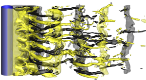
The canonical case of steady approaching flow past a smooth and slender circular cylinder (referred to as flow past a circular cylinder hereafter) has been a classical topic in fluid mechanics owing to its physical complexity and extensive engineering applications. The sole governing parameter of the flow is the Reynolds number Re (= UD/ν), which is defined based on the velocity of the approaching flow (U), the diameter of the cylinder (D) and the kinematic viscosity of the fluid (ν). Despite its geometric simplicity, complex evolutions of the flow with increasing Re have been discovered, e.g. flow separation, vortex shedding, three-dimensional (3-D) wake transition and transition to turbulence in the wake, the separating shear layer and the boundary layer (see e.g. Williamson Reference Williamson1996; Zdravkovich Reference Zdravkovich1997). Figure 1 illustrates an instantaneous 3-D turbulent wake structure at Re = 1000, where the spanwise vorticity (ωz) and streamwise vorticity (ωx) are defined in a non-dimensional form:
 \begin{gather}{\omega _z} = \left( {\frac{{\partial v}}{{\partial x}} - \frac{{\partial u}}{{\partial y}}} \right)\frac{D}{U},\end{gather}
 \begin{gather}{\omega _x} = \left( {\frac{{\partial w}}{{\partial y}} - \frac{{\partial v}}{{\partial z}}} \right)\frac{D}{U},\end{gather}
where (x, y, z) and (u, v, w) are the Cartesian coordinates and velocity components in the streamwise, transverse (cross-flow) and spanwise directions, respectively.

Figure 1. Instantaneous vorticity field in the turbulent wake of a circular cylinder at Re = 1000: (a) iso-surfaces of spanwise (translucent) and streamwise (opaque) vortices, (b) iso-surfaces of spanwise vortices only and (c) iso-surfaces of streamwise vortices only. Red and blue represent positive and negative vorticity values of ±4, respectively. The flow is from left to right past the cylinder on the left.
The above-mentioned flow characteristics are generally observed close to the cylinder. An exception is the turbulent wake observed at  $Re\mathrm{\ \mathbin{\lower.3ex\hbox{$\buildrel> \over {\smash{\scriptstyle\sim}\vphantom{_x}}$}}\ }260$ (Williamson Reference Williamson1996), which develops into the far-wake region. Not surprisingly, the turbulent intermediate and far wake have been far less studied in the literature than other flow characteristics, which is likely due to the difficulty in measuring the turbulent quantities accurately by physical experiments, and the high computational cost associated with resolving the intermediate and far wake in 3-D numerical simulations.
In addition to the more well-known quantity of turbulent kinetic energy, another major quantity governing the turbulent wake is the kinetic energy dissipation rate, which was examined by several experimental studies in the literature (e.g. Browne, Antonia & Shah Reference Browne, Antonia and Shah1987; George & Hussein Reference George and Hussein1991; T. Zhou et al. Reference Zhou, Zhou, Yiu and Chua2003; Ducci et al. Reference Ducci, Konstantinidis, Balabani and Yianneskis2005; Chen et al. Reference Chen, Zhou, Antonia and Zhou2018). For the turbulent wake, the velocity and the kinetic energy dissipation rate can be decomposed into three components, i.e. a mean (time-averaged) component, a coherent fluctuation component associated with the primary vortices and a remainder associated with the smaller-scale structures (Reynolds & Hussain Reference Reynolds and Hussain1972; Cantwell & Coles Reference Cantwell and Coles1983; Elsner & Elsner Reference Elsner and Elsner1996). The remainder consists of two parts, i.e. an incoherent fluctuation associated with the random turbulence and a coherent fluctuation associated with the rib-like mode B streamwise vortices (Williamson Reference Williamson1996; Zhang, Zhou & Antonia Reference Zhang, Zhou and Antonia2000) which are randomly distributed along the spanwise direction (figure 1c). For an instantaneous flow quantity s (e.g. a velocity component), the three components are denoted sm,  $\tilde{s}$ and sr, respectively, and the total fluctuation is denoted s′, i.e.
 \begin{equation}s = {s_m} + \tilde{s} + {s_r} = {s_m} + s^{\prime}.\end{equation}
Based on the assumption that the two fluctuation components  $\tilde{s}$ and sr are uncorrelated (Reynolds & Hussain Reference Reynolds and Hussain1972), the total kinetic energy dissipation rate ε can be decomposed into the contributions from the mean flow, the coherent primary vortices and the remainder, i.e. (Elsner & Elsner Reference Elsner and Elsner1996)
 \begin{equation}\varepsilon = {\varepsilon _m} + \tilde{\varepsilon } + {\varepsilon _r} = {\varepsilon _m} + \varepsilon ^{\prime},\end{equation}
where
 \begin{gather}\varepsilon = \nu \overline {\frac{{\partial {u_i}}}{{\partial {x_j}}}\left( {\frac{{\partial {u_i}}}{{\partial {x_j}}} + \frac{{\partial {u_j}}}{{\partial {x_i}}}} \right)} ,\end{gather}
 \begin{gather}{\varepsilon _m} = \nu \frac{{\partial {u_{m,}}_i}}{{\partial {x_j}}}\left( {\frac{{\partial {u_{m,}}_i}}{{\partial {x_j}}} + \frac{{\partial {u_{m,}}_j}}{{\partial {x_i}}}} \right),\end{gather}
 \begin{gather}\tilde{\varepsilon } = \nu \overline {\frac{{\partial {{\tilde{u}}_i}}}{{\partial {x_j}}}\left( {\frac{{\partial {{\tilde{u}}_i}}}{{\partial {x_j}}} + \frac{{\partial {{\tilde{u}}_j}}}{{\partial {x_i}}}} \right)} ,\end{gather}
 \begin{gather}{\varepsilon _r} = \nu \overline {\frac{{\partial {u_{i,r}}}}{{\partial {x_j}}}\left( {\frac{{\partial {u_{i,r}}}}{{\partial {x_j}}} + \frac{{\partial {u_{j,r}}}}{{\partial {x_i}}}} \right)} ,\end{gather}
 \begin{gather}\varepsilon ^{\prime} = \nu \overline {\frac{{\partial {{u^{\prime}}_i}}}{{\partial {x_j}}}\left( {\frac{{\partial {{u^{\prime}}_i}}}{{\partial {x_j}}} + \frac{{\partial {{u^{\prime}}_j}}}{{\partial {x_i}}}} \right)} ,\end{gather}
where an overbar denotes a mean value (and εm is a mean value by definition), ui is the velocity component in the direction xi and i = 1, 2 and 3 represent the streamwise, transverse and spanwise directions, respectively. In Appendix A, a numerical validation of the relationship  $\varepsilon = {\varepsilon _m} + \tilde{\varepsilon } + {\varepsilon _r}$ is reported based on the present numerical results.
By decomposing ε′ into  $\tilde{\varepsilon }$ and εr, Chen et al. (Reference Chen, Zhou, Antonia and Zhou2018) quantified the transverse distribution of coherent contribution
  $\tilde{\varepsilon }/(\tilde{\varepsilon } + {\varepsilon _r})$ at x/D = 10, 20 and 40 of the turbulent wake at Re = 2500. They showed that the maximum coherent contribution at x/D = 10 was ~9 % (at y/D = 0.6), while the maximum coherent contribution at x/D = 20 was ~4 % (at y/D = 0.2). Similarly, Ducci et al. (Reference Ducci, Konstantinidis, Balabani and Yianneskis2005) examined the turbulent wake at Re = 6700 and 7200, and found that at x/D = 10 the coherent component accounted for 10 %–15 % of the total dissipation rate.
The minor coherent contribution at x/D > 20 (Chen et al. Reference Chen, Zhou, Antonia and Zhou2018) may explain why other experimental studies, which focused mainly on the relatively far wake, did not quantify  $\tilde{\varepsilon }$ and εr and instead used ε′ directly. Indeed, the focus of most of the experimental studies was on an appropriate approximation of the dissipation rate using simplified surrogates, since it was extremely difficult to measure all 12 velocity derivative terms constituting the dissipation rate in physical experiments (Browne et al. Reference Browne, Antonia and Shah1987; Chen et al. Reference Chen, Zhou, Antonia and Zhou2018). As summarised by Chen et al. (Reference Chen, Zhou, Antonia and Zhou2018), commonly used surrogates include local isotropy (Taylor Reference Taylor1935), local axisymmetry with respect to the streamwise direction x (George & Hussein Reference George and Hussein1991), local homogeneity (Taylor Reference Taylor1935) and homogeneity in the y–z plane (Zhu & Antonia Reference Zhu and Antonia1997). The four surrogates are expressed as follows, where (u 1, u 2, u 3) and (x 1, x 2, x 3) are used interchangeably with (u, v, w) and (x, y, z), respectively:
 \begin{gather}{\varepsilon ^{\prime}_{iso}} = 15\nu \overline {{{\left( {\frac{{\partial u^{\prime}}}{{\partial x}}} \right)}^2}} ,\end{gather}
 \begin{gather}{\varepsilon ^{\prime}_{axis}} = \nu \left[ {\frac{5}{3}\overline {{{\left( {\frac{{\partial u^{\prime}}}{{\partial x}}} \right)}^2}} + 2\overline {{{\left( {\frac{{\partial u^{\prime}}}{{\partial z}}} \right)}^2}} + 2\overline {{{\left( {\frac{{\partial v^{\prime}}}{{\partial x}}} \right)}^2}} + \frac{8}{3}\overline {{{\left( {\frac{{\partial v^{\prime}}}{{\partial z}}} \right)}^2}} } \right],\end{gather}
 \begin{gather}{\varepsilon ^{\prime}_{hom}} = \nu \overline {\frac{{\partial {{u^{\prime}}_i}}}{{\partial {x_j}}}\frac{{\partial {{u^{\prime}}_i}}}{{\partial {x_j}}}} ,\end{gather}
 \begin{gather} {{\varepsilon ^{\prime}}_{yz}} =\nu \left[ {4\overline {{{\left( {\dfrac{{\partial u^{\prime}}}{{\partial x}}} \right)}^2}} + \overline {{{\left( {\dfrac{{\partial u^{\prime}}}{{\partial y}}} \right)}^2}} + \overline {{{\left( {\dfrac{{\partial u^{\prime}}}{{\partial z}}} \right)}^2}} + \overline {{{\left( {\dfrac{{\partial v^{\prime}}}{{\partial x}}} \right)}^2}} + \overline {{{\left( {\dfrac{{\partial v^{\prime}}}{{\partial z}}} \right)}^2}} + } \right.\overline {{{\left( {\dfrac{{\partial w^{\prime}}}{{\partial x}}} \right)}^2}} + \overline {{{\left( {\dfrac{{\partial w^{\prime}}}{{\partial y}}} \right)}^2}} \nonumber\\ \hspace{-3.3pc} \left. +\,2\overline {\left( {\dfrac{{\partial u^{\prime}}}{{\partial y}}} \right)\left( {\dfrac{{\partial v^{\prime}}}{{\partial x}}} \right)} + 2\overline {\left( {\dfrac{{\partial u^{\prime}}}{{\partial z}}} \right)\left( {\dfrac{{\partial w^{\prime}}}{{\partial x}}} \right)} - 2\overline {\left( {\dfrac{{\partial v^{\prime}}}{{\partial z}}} \right)\left( {\dfrac{{\partial w^{\prime}}}{{\partial y}}} \right)} \right]. \end{gather}
Not surprisingly, the surrogate of local isotropy, which requires the measurement of only one of the 12 terms, is often reported to be inaccurate (e.g. Browne et al. Reference Browne, Antonia and Shah1987; George & Hussein Reference George and Hussein1991). On the other hand, it is difficult to evaluate the accuracy of the other three surrogates, because the true value of ε′ is almost impossible to be measured from physical experiments (which involves the use of highly complex hotwire probes or 3-D particle image velocimetry techniques, albeit still limited by spatial and temporal resolutions). Even for the velocity gradients which are measurable by the experiments, moderate errors may arise from, for example, limited spatial resolution of the probes for measuring the velocity gradients and the use of Taylor's hypothesis (T. Zhou et al. Reference Zhou, Zhou, Yiu and Chua2003). For example, T. Zhou et al. (Reference Zhou, Zhou, Yiu and Chua2003) and Chen et al. (Reference Chen, Zhou, Antonia and Zhou2018) stated that in their experiments the velocity gradients were underestimated by approximately 18 %–7 % at x/D = 10–40.
To overcome the experimental limitations, direct numerical simulation (DNS) is used in the present study to quantify the full energy dissipation rate ε′ and its surrogates and to evaluate their adequacy in representing ε′. Chen et al. (Reference Chen, Zhou, Antonia and Zhou2018) also commented on the lack of numerical datasets for evaluating the true value of ε′, which justifies the necessity of the present study. The present DNS results provide guidance and support to experimental studies on the use of appropriate surrogates for ε′. The present study also examines whether the turbulent wake is indeed locally isotropic, axisymmetric and homogeneous.
2. Numerical model
2.1. Numerical method
The governing equations for flow past a circular cylinder are the continuity and incompressible Navier–Stokes equations:
 \begin{gather}\frac{{\partial {u_i}}}{{\partial {x_i}}} = 0,\end{gather}
 \begin{gather}\frac{{\partial {u_i}}}{{\partial t}} + {u_j}\frac{{\partial {u_i}}}{{\partial {x_j}}} ={-} \frac{{\partial p}}{{\partial {x_i}}} + \nu \frac{{{\partial ^2}{u_i}}}{{\partial {x_j}\partial {x_j}}},\end{gather}
where t is time and p is kinematic pressure (pressure divided by fluid density).
The governing equations were solved by the open-source code Nektar++ (Cantwell et al. Reference Cantwell2015) through the so-called quasi-3-D approach. Specifically, the flow in the x–y plane was solved by a high-order spectral/hp element method (Karniadakis & Sherwin Reference Karniadakis and Sherwin2005), while that in the spanwise direction was represented by a Fourier expansion (Karniadakis Reference Karniadakis1990). This approach provided a higher computational efficiency than conventional finite element and similar methods (Cantwell et al. Reference Cantwell2015; Moxey et al. Reference Moxey2020). The numerical simulations adopted the unsteady Navier–Stokes solver embedded in Nektar++, together with the velocity correction scheme (Karniadakis, Israeli & Orszag Reference Karniadakis, Israeli and Orszag1991), a second-order implicit–explicit (IMEX) time-integration scheme and a continuous Galerkin projection. The spectral vanishing viscosity (SVV) technique proposed by Kirby and Sherwin (Reference Kirby and Sherwin2006) was used to stabilise the solution. The SVV cut-off ratio was set to 0.9 (with 1.0 being no effect on the simulation), while the SVV diffusion coefficient was set to 0.1 (with 0 being no effect).
2.2. Computational domain and mesh
The present study investigated mainly the turbulent wake at Re = 1000. A rectangular computational domain was adopted for the x–y plane. The centre of the cylinder was placed at (x, y) = (0, 0). The computational domain size was −30 ≤ x/D ≤ 120 in the streamwise direction and −30 ≤ y/D ≤ 30 in the transverse direction.
Figure 2 shows the macro-element mesh near the cylinder. The perimeter of the cylinder was discretised equally with 48 macro-elements. The first layer of macro-elements had a radial size of 0.00553D. To resolve the wake characteristics, the streamwise size of the macro-elements for x/D = 4–120 was fixed at 0.2D. The total number of macro-elements in the x–y plane was 26 922. Each macro-element contained a further quadrilateral expansion using fourth-order Lagrange polynomials (denoted Np = 4).

Figure 2. The macro-element mesh near the cylinder.
The 3-D mesh was constructed by using 128 Fourier planes over the spanwise domain length Lz/D = 6. The adequacy of Lz/D = 6 was demonstrated by Jiang & Cheng (Reference Jiang and Cheng2017) based on a comparison of Lz/D = 6 and 12 at Re = 1000. The adequacy of 128 Fourier planes for Lz/D = 6 was demonstrated by Jiang & Cheng (Reference Jiang and Cheng2021) at Re = 3900 and was expected to be applicable to Re = 1000.
The boundary conditions for the computational domain were specified as follows. At the inlet (x/D = −30) and transverse (y/D = ±30) boundaries, a uniform velocity (u, v, w) = (U, 0, 0) was specified, together with a high-order Neumann condition for the pressure (Karniadakis et al. Reference Karniadakis, Israeli and Orszag1991). At the outlet (x/D = 120) boundary, the velocity was set to the Neumann condition, while the pressure was specified as a reference value of zero. At the cylinder surface, the no-slip condition was used. At the two boundaries perpendicular to the spanwise direction, periodic boundary conditions were applied.
At the beginning of the simulation, the internal flow followed an impulsive start. The non-dimensional time-step size (Δt* = ΔtU/D) was 0.003125, which corresponded to a Courant–Friedrichs–Lewy (CFL) limit of 0.53. Each case was simulated for at least 1000 non-dimensional time units (defined as t* = tU/D), with the first 400 time units used to phase out the transients and the remainder for the statistics and analysis. The numerical simulations were conducted on a Cray XC40 system supercomputer. For the reference case with Np = 4, the computational cost for 1000 time units was approximately 82 200 core hours (a parallel computation using 120 processors and approximately 685 hours of wall-clock time for each processor).
Appendix B reports a detailed mesh convergence study, which includes separate examinations of the effects of overall mesh resolution, element stretching in the wake region, statistical time period, sample interval, the SVV technique and the time integration technique on the prediction of the mean kinetic energy dissipation rate ε. The reference case examined in Appendix B employed the mesh shown in figure 2 (with Np = 4 and no element stretching along the wake), a statistical time period of 100T (T being the vortex shedding period), a sample interval of T/16 (i.e. a total of 1600 fields over the statistical time period of 100T) and a non-dimensional time-step size of 0.003125. Based on Appendix B, the reference case was deemed adequate for the present study. Nevertheless, for the main body of the present study the ε value (and the corresponding velocity derivative terms) was obtained with a doubled statistical time period of 200T (i.e. a total of 3200 fields), because the data were readily available from the mesh convergence study. In addition to the time average, the results were also averaged along the spanwise direction and between the two sides of the wake centreline.
2.3. Phase-averaging technique
A reliable phase-averaging technique is needed to extract the coherent structures. The present phase-averaging technique generally follows that used by Matsumura & Antonia (Reference Matsumura and Antonia1993), Y. Zhou, Zhang & Yiu (Reference Zhou, Zhang and Yiu2002) and Chen et al. (Reference Chen, Zhou, Antonia and Zhou2018) for wind-tunnel experimental results. However, some modifications of the technique are made to facilitate processing of the present numerical results, because the present numerical data consist of the output of a large number of instantaneous flow fields, whereas wind-tunnel data are generally sampled at selected discrete points.
To extract the coherent structures at a specific streamwise location in the wake, the time history of the transverse velocity v sampled at this streamwise location and y/D = 1 is used as a reference signal. To maximise the length of statistical data, the reference signals are taken at four equally spaced spanwise locations (i.e. z/D = 0, 1.5, 3 and 4.5) and are processed individually. Each v signal is filtered using a fourth-order Butterworth filter with the centre frequency set at the primary vortex shedding frequency (e.g. Y. Zhou et al. Reference Zhou, Zhang and Yiu2002; Chen et al. Reference Chen, Zhou, Antonia and Zhou2018), as identified from the fast Fourier transform of the signal. Figure 3(a) illustrates the v signal sampled at (x/D, y/D, z/D) = (10, 1, 3) and the corresponding filtered signal. Based on the filtered signal, the local peaks in the time history are set to phase φ = 0, while the local troughs are set to phase φ =  ${\rm \pi}$. Between each peak and trough, the time range is equally divided into 8 intervals, such that a period from a peak to the next peak is divided into 16 intervals. From a peak to the next peak, the selected phases are set to φ = n × (2
 ${\rm \pi}$/16), where n is an integer from 0 to 16. The instantaneous flow fields at the selected phases are then used for the phase average. The phase average (denoted by
  $\langle \cdot \rangle$) of a flow field u at a specific phase (denoted by the subscript p) is calculated as
 \begin{equation}{\langle \boldsymbol{u}\rangle _p} = \frac{1}{{{N_p}}}\sum\limits_{i = 1}^{{N_p}} {{\boldsymbol{u}_{p,i}}} ,\end{equation}
where Np is the number of periods for the phase average. Finally, the phase-averaged flow fields obtained individually at each of the four spanwise locations are further averaged to obtain the final phase-averaged flow field. For the final phase-averaged flow field, only the area near the streamwise location where the v signals are sampled is meaningful.

Figure 3. Reference signals for the phase average: (a) the v signal sampled at (x/D, y/D, z/D) = (10, 1, 3) and (b) the time history of CL. To facilitate comparison between the original and filtered signals in (a), the filtered results are multiplied by 5.246, such that the standard deviation of the two signals is the same, while the phase is unchanged.
Similarly, the time history of the lift coefficient (CL) on the cylinder can be used as a reference signal for a phase average to extract the coherent structures near x/D = 0. Since the CL signal varies smoothly over time (figure 3b), no filter is used. For this phase-averaged flow field, only the area near x/D = 0 is meaningful.
At a specific phase p, the coherent component of the velocity field  $({\tilde{\boldsymbol{u}}_p})$ is determined based on the final phase-averaged velocity field
  $({\langle \boldsymbol{u}\rangle _p})$ and the time- and span-averaged velocity field (um), i.e.
 \begin{equation}{\tilde{\boldsymbol{u}}_p} = {\langle \boldsymbol{u}\rangle _p} - {\boldsymbol{u}_m}.\end{equation}
The coherent component of the dissipation rate at phase p ( ${\tilde{\varepsilon }_p}$) is calculated by substituting
  ${\tilde{\boldsymbol{u}}_p}$ into (1.7). Finally, the averaged coherent contribution of the dissipation rate (
 $\tilde{\varepsilon }$) is determined as an average of the
  ${\tilde{\varepsilon }_p}$ values over the 16 selected phases over the vortex shedding period. This approach is similar to the ‘structural averaging’ technique used by Y. Zhou et al. (Reference Zhou, Zhang and Yiu2002) and Chen et al. (Reference Chen, Zhou, Antonia and Zhou2018) for experimental datasets.
3. Numerical results
3.1. Pattern of the primary vortex street
Following the phase-averaging technique introduced in § 2.3, it is interesting to examine the differences of the phase-averaged flow fields obtained based on the reference signals sampled at different x/D. This comparison sheds light on how well a phase-averaged flow field obtained based on the reference signal at a specific x/D represents the flow over a range of x/D. For example, the CL signal was commonly used in previous numerical and particle image velocimetry experimental studies in obtaining the phase-averaged flow field, and it is unclear to what extent this phase-averaged flow field represented the actual wake pattern over a range of x/D.
Figure 4 shows the phase-averaged spanwise vorticity fields in the turbulent wake of Re = 1000, determined based on the CL signal (figure 4a) and the v signals sampled at x/D = 10 (figure 4b) and x/D = 20 (figure 4c). The vorticity fields are shown at a phase where the reference signal reaches its maximum. Qualitatively, the three vorticity fields show similar patterns, where the primary vortex street gradually decays with distance downstream. The decay of the primary vortex street for the three cases shown in figure 4(a–c) is quantified by the streamwise variation of the peak vorticity of vortices in figure 5(a–c), respectively. The fitted curves in figure 5(a–c) are further summarised in figure 5(d). As expected, the CL signal gives rise to the largest peak vorticity very close to the cylinder, while the v signals sampled at x/D = 10 and 20 yield the largest peak vorticity at x/D = 10 and 20, respectively (highlighted by the open circles in figure 5d). Based on the CL signal, the peak vorticity values at x/D = 10 and 20 are under-predicted by 20 % and 27 %, respectively. Based on the v signal sampled at x/D = 10, the peak vorticity at x/D = 20 is under-predicted by a smaller extent of 8 %. Based on the v signal sampled at x/D = 20, the peak vorticity at x/D = 10 is under-predicted by 44 %. Therefore, the quantitative validity of a phase-averaged flow field is well within 10D of the streamwise location for the reference signal (especially when extending upstream).

Figure 4. Phase-averaged spanwise vorticity field in the turbulent wake of Re = 1000, determined based on the reference signal of (a) the lift coefficient (i.e. at x/D ~ 0), (b) transverse velocity v sampled at x/D = 10 and (c) transverse velocity v sampled at x/D = 20. All the vorticity fields are shown at a phase where the reference signal reaches its maximum.

Figure 5. Streamwise variation of the peak vorticity of the phase-averaged vortices in the turbulent wake of Re = 1000, determined based on the reference signal of (a) the lift coefficient (i.e. at x/D ~ 0), (b) transverse velocity v sampled at x/D = 10 and (c) transverse velocity v sampled at x/D = 20. (d) A comparison of the present results with those reported by Hussain & Hayakawa (Reference Hussain and Hayakawa1987), Y. Zhou et al. (Reference Zhou, Zhang and Yiu2002), and T. Zhou et al. (Reference Zhou, Zhou, Yiu and Chua2003).
Figure 5(d) also shows a comparison of the present results for the turbulent wake of Re = 1000 (the open circles) with those reported by Hussain & Hayakawa (Reference Hussain and Hayakawa1987), Y. Zhou et al. (Reference Zhou, Zhang and Yiu2002) and T. Zhou et al. (Reference Zhou, Zhou, Yiu and Chua2003) based on physical experiments at different Re values. The relatively good agreement between the present results and those reported in the literature (especially Y. Zhou et al. Reference Zhou, Zhang and Yiu2002) suggests that the primary vortex street may undergo a similar decay with distance downstream over a range of subcritical Re.
Similar to the determination of the peak vorticity of the phase-averaged vortices at x/D = 10 and 20 in figure 5, table 1 summarises the transverse location of the peak vorticity (yc/D) and the advection velocity of the vortex (Uc/U) at y = yc for x/D = 10 and 20. The present results agree relatively well with the experimental results of Y. Zhou et al. (Reference Zhou, Zhang and Yiu2002), T. Zhou et al. (Reference Zhou, Zhou, Yiu and Chua2003) and Hussain & Hayakawa (Reference Hussain and Hayakawa1987).
Table 1. Characteristics of the phase-averaged vortices at x/D = 10 and 20.

3.2. Spectral analysis of decay of the primary vortex street
In addition to the streamwise variation of the peak vorticity of the phase-averaged vortices shown in figure 5(d), the decay of the primary vortex street with distance downstream can also be quantified by the frequency spectra of v sampled at various streamwise locations along y/D = 0 (figure 6) and y/D = 1.5 (figure 7). The frequency spectra are determined from the fast Fourier transform of the time histories of v, where A and f denote the amplitude and frequency of v, respectively. Each frequency spectrum shown in figures 6 and 7 is an average of the frequency spectra derived from the time histories of v sampled at 16 equally spaced spanwise locations. Each time history of v is sampled over a time period of 100T with a sample interval of 6Δt* (= 0.01875). The resultant frequency spectrum has a frequency resolution of ΔfD/U = 0.00207.

Figure 6. Frequency spectra of v sampled at various streamwise locations along the wake centreline (y/D = 0) for the turbulent wake of Re = 1000: (a) x/D = 5–30 and (b) x/D = 40–110.

Figure 7. Frequency spectra of v sampled at various streamwise locations along y/D = 1.5 for the turbulent wake of Re = 1000: (a) x/D = 5–30 and (b) x/D = 30–110.
As shown in figures 6(a) and 7(a), the relatively near wake of the cylinder is dominated by a well-defined frequency corresponding to the primary vortex shedding (i.e. St). The decrease in the amplitude of v at St with distance downstream is quantified in figure 8(a). In particular, an exponential decay of the amplitude at St is observed for y/D = 0 over x/D = 5–30. Based on a curve fitting of this range, the decay rate of the primary vortex street is 0.0380 decades/D, where decade stands for an order of magnitude in A. Figure 9 summarises the decay rates for different Re values, including those determined in the present study and those by Cimbala et al. (Reference Cimbala, Nagib and Roshko1988) using the v signal. The decay rate increases approximately linearly over the range of Re investigated.

Figure 8. Streamwise variations of (a) the amplitude of v at St and (b) the normalised amplitude of v at St.

Figure 9. Decay rate of the primary vortices predicted at different Re values. The decay rate is determined as the decrease in the spectral amplitude of v at St with distance downstream.
As shown in figures 6(b) and 7(b) and further quantified in figure 8(a), the amplitude at St decreases gradually with distance downstream and dives into the noise level (quantified by the largest amplitude other than that at St). Based on a linear interpolation, the frequency peak at St disappears at x/D = 64 for y/D = 0 but earlier at x/D = 49 for y/D = 1.5 (a convergence check of the x/D value with respect to several key numerical parameters is reported in Appendix C). The reason for the difference is that although the positive (or negative) primary vortices mainly travel along y/D ~ 1.5 (or y/D ~ −1.5) over the streamwise range of at least x/D ~ 50–60 (figure 4), the alternate passage of the positive and negative vortices near the wake centreline still induces a larger amplitude of v at St at y/D = 0 than that at y/D = 1.5 (figure 8a), such that the St peak can be detected more downstream at y/D = 0.
Similarly, Roshko (Reference Roshko1954) found that for the turbulent wakes of Re = 500–4000, the discrete energy at St disappeared and the wake became completely turbulent at x/D = 40–50. Compared with the present results, the slightly smaller x/D identified by Roshko (Reference Roshko1954) was likely affected by the transverse locations of y/D > 1.5 for the measurement of the frequency spectra at x/D = 24 and 48. On the other hand, Browne, Antonia & Shah (Reference Browne, Antonia and Shah1989) found that for the turbulent wake of Re = 1170, the discrete energy at St disappeared at x/D ~ 75, which was partly because their measurement was taken at the transverse location of maximum signal strength.
As the wake becomes increasingly turbulent with distance downstream, the energy in the wake may transfer from St to other frequencies. In order to reveal the energy transfer, the amplitude of v at St (figure 8a) is normalised by  $\sqrt {2\overline {v^{\prime}v^{\prime}} }$ (figure 8b). Such a normalisation removes the influence of the fluctuating amplitude of the v signal and reveals the relative strengths of different frequency components. For example, when the time history of v is sinusoidal with a single frequency St and arbitrary amplitude, the normalised amplitude becomes 1.0. For the laminar primary vortex street, the normalised amplitude is very close to 1.0 (Jiang & Cheng Reference Jiang and Cheng2019). For the turbulent wake at Re = 1000, however, the normalised amplitude of v at St decreases monotonically with distance downstream (figure 8b), which suggests that the velocity fluctuation is decreasingly contributed by the primary vortices and increasingly contributed by the turbulence.
3.3. Three components of the kinetic energy dissipation rate
As introduced in § 1, the total kinetic energy dissipation rate ε consists of the contributions from the mean flow, the coherent primary vortices and the remainder, which are denoted εm,  $\tilde{\varepsilon }$ and εr and determined by (1.6)–(1.8), respectively. Owing to the random distribution of the rib-like streamwise vortices (figure 1c) and the associated turbulence along the spanwise direction, at any specific point in the flow field the mean spanwise velocity and the phase-averaged spanwise velocity should be zero, such that (1.6) and (1.7) can be reduced to
 \begin{gather}{\varepsilon _m} = \nu \frac{{\partial {u_{m,}}_i}}{{\partial {x_j}}}\left( {\frac{{\partial {u_{m,}}_i}}{{\partial {x_j}}} + \frac{{\partial {u_{m,}}_j}}{{\partial {x_i}}}} \right)\quad (i,j = 1,\textrm{ }2),\end{gather}
 \begin{gather}\tilde{\varepsilon } = \nu \overline {\frac{{\partial {{\tilde{u}}_i}}}{{\partial {x_j}}}\left( {\frac{{\partial {{\tilde{u}}_i}}}{{\partial {x_j}}} + \frac{{\partial {{\tilde{u}}_j}}}{{\partial {x_i}}}} \right)} \quad (i,j = 1,2).\end{gather}
Practically, the εm and  $\tilde{\varepsilon }$ values determined by (1.6) and (1.7) may be slightly larger than those determined by (3.1) and (3.2). This is because the time-averaged and phase-averaged flows are obtained from finite statistical time periods, where small degrees of spanwise velocity (of the order of 0.01U) may exist and contribute undesirably to εm and
  $\tilde{\varepsilon }$. To eliminate this effect, the present study uses (3.1) and (3.2) to calculate εm and
  $\tilde{\varepsilon }$. To further improve the statistical convergence, (3.1) is calculated based on the time- and span-averaged velocity field, while (3.2) is calculated based on the procedures introduced in § 2.3 (calculated at four equally spaced spanwise locations). To maintain conservation of the total dissipation rate, εr is calculated as
 \begin{equation}{\varepsilon _r} = \varepsilon - {\varepsilon _m} - \tilde{\varepsilon },\end{equation}
where ε is calculated by (1.5) using the instantaneous 3-D velocity fields.
Figure 10 shows the span-averaged fields of εm,  $\tilde{\varepsilon }$ and εr for the turbulent wake of Re = 1000, where the phase average is based on the CL signal. It is also checked that by using the v signal sampled at x/D = 10, the
  $\tilde{\varepsilon }$ and εr fields are qualitatively similar. As shown in figure 10(a), the εm component is concentrated in the boundary layer and the separating shear layer, which is in accordance with the mean shear of the flow around the cylinder. In contrast, the
  $\tilde{\varepsilon }$ and εr components shown in figure 10(b,c) develop in the wake region. The
  $\tilde{\varepsilon }$ field displays two peak regions away from the wake centreline, while the εr field peaks at the wake centreline (for x/D
  $\gtrsim$ 5). The different peak regions for the
  $\tilde{\varepsilon }$ and εr components can be explained based on figure 22(c,d) in § 3.8, where the spatial distributions of the phase-averaged fields are presented.

Figure 10. Span-averaged fields of (a)  ${\varepsilon _m}D/{U^3}$, (b)
  $\tilde{\varepsilon }D/{U^3}$ and (c)
  ${\varepsilon _r}D/{U^3}$.
The  $\tilde{\varepsilon }$ and εr fields shown in figure 10(b,c) are qualitative patterns. Quantitatively, the transverse distribution of
  $\tilde{\varepsilon }$ at a specific x/D should be determined by extracting the coherent structures based on the v signals sampled at the corresponding x/D. For example, figure 11(a) illustrates the transverse distributions of
  $\tilde{\varepsilon }$ at x/D = 10 determined based on different reference signals. The largest
  $\tilde{\varepsilon }$ values at x/D = 10 are determined based on the v signals sampled at x/D = 10. Figure 11(a) also illustrates the transverse distributions of εm, εr and ε at x/D = 10, which indicates that at a specific x/D, the three components of the dissipation rate (εm,
  $\tilde{\varepsilon }$ and εr) may peak at different transverse locations (also shown qualitatively in figure 10). Therefore, it is less meaningful to compare their values at a same transverse location (as was done in several previous studies). Instead, the contribution of each component at a specific x/D is quantified through integrating the corresponding component along the y direction, such that its percentage contribution to the total ε can be determined.

Figure 11. (a) Transverse distribution of different components of the dissipation rate at x/D = 10. (b–d) Streamwise variation of the integrated dissipation rate: (b) the coherent component  $\tilde{\varepsilon }$ determined based on different reference signals, (c) different components of the dissipation rate and (d) percentage contribution of different components of the dissipation rate.
Figure 11(b) shows the streamwise variations of the integrated  $\tilde{\varepsilon }$ determined based on different reference signals. The effect of different reference signals is similar to that observed for the streamwise variation of the peak vorticity in figure 5(d), where the v signals sampled at x/D = 10 and 20 yield the largest results at x/D = 10 and 20, respectively (denoted by filled circles). Based on the CL signal, the integrated
  $\tilde{\varepsilon }$ at x/D = 10 and 20 are under-predicted by 17 % and 39 %, respectively, which justifies the necessity of calculating
  $\tilde{\varepsilon }$ based on the coherent structures extracted at the corresponding x/D.
Figure 11(c) shows the actual integrated  $\tilde{\varepsilon }$ at x/D = 10 and 20, together with the integrated ε, εm and ε′ (= ε − εm) values at various x/D. The integrated ε, εm and ε′ values are not limited at x/D = 10 and 20, because they are not related to how the coherent structures are extracted. The εm component, which is associated with the mean shear around the cylinder, decreases drastically and monotonically with distance downstream. The total fluctuation component ε′ peaks at x/D ~ 1.5, which is consistent with the emergence of the primary and secondary vortices and the associated turbulence in the near wake, and then gradually decreases downstream.
Based on the results shown in figure 11(c), the percentage contributions of εm and  $\tilde{\varepsilon }$ to the total ε are shown in figure 11(d). The percentage contribution of the εm component quickly drops to ~1 % at x/D ~ 4 and remains at ~1 % further downstream. The
  $\tilde{\varepsilon }$ component, which is associated with the coherent primary vortices, accounts for only 4.2 % and 2.0 % of the total ε at x/D = 10 and 20, respectively. In contrast, the remainder, which is induced by the rib-like streamwise vortices and the associated random turbulence that develop only in the 3-D turbulent wake, accounts for the majority of the total ε for almost the entire wake (beyond the immediate neighbourhood of the cylinder), e.g. 95 % and 97 % for x/D = 10 and 20, respectively.
3.4. Twelve velocity derivative terms constituting the dissipation rate
In this section, the 12 velocity derivative terms constituting the dissipation rate are examined separately. To facilitate comparison of the present results with the experimental results of Chen et al. (Reference Chen, Zhou, Antonia and Zhou2018), the total fluctuation component of the dissipation rate ε′ is presented for both cases. The 12 velocity derivative terms for ε′ are given on the right-hand side of the following equation:
 \begin{align} \dfrac{{\varepsilon ^{\prime}}}{\nu }&=2\overline {{{\left( {\dfrac{{\partial u^{\prime}}}{{\partial x}}} \right)}^2}} + \overline {{{\left( {\dfrac{{\partial v^{\prime}}}{{\partial x}}} \right)}^2}} + \overline {{{\left( {\dfrac{{\partial w^{\prime}}}{{\partial x}}} \right)}^2}} + \overline {{{\left( {\dfrac{{\partial u^{\prime}}}{{\partial y}}} \right)}^2}} + 2\overline {{{\left( {\dfrac{{\partial v^{\prime}}}{{\partial y}}} \right)}^2}} + \overline {{{\left( {\dfrac{{\partial w^{\prime}}}{{\partial y}}} \right)}^2}} \nonumber\\ &\quad + \overline {{{\left( {\dfrac{{\partial u^{\prime}}}{{\partial z}}} \right)}^2}} + \overline {{{\left( {\dfrac{{\partial v^{\prime}}}{{\partial z}}} \right)}^2}} + 2\overline {{{\left( {\dfrac{{\partial w^{\prime}}}{{\partial z}}} \right)}^2}} + 2\overline {\dfrac{{\partial u^{\prime}}}{{\partial y}}\dfrac{{\partial v^{\prime}}}{{\partial x}}} + 2\overline {\dfrac{{\partial u^{\prime}}}{{\partial z}}\dfrac{{\partial w^{\prime}}}{{\partial x}}} + 2\overline {\dfrac{{\partial v^{\prime}}}{{\partial z}}\dfrac{{\partial w^{\prime}}}{{\partial y}}}. \end{align}
 Figure 12 illustrates the transverse distribution of the term  $2\overline {{{(\partial u^{\prime}/\partial x)}^2}}$ at x/D = 10, 20 and 40 in a turbulent wake of Re = 1000. After normalising the term into
  $2\overline {{{(\partial u^{\prime}/\partial x)}^2}} /{(U/D)^2}$, a comparison is made between the present results and the experimental results of Chen et al. (Reference Chen, Zhou, Antonia and Zhou2018) at Re = 2500. The reason why the term
  $2\overline {{{(\partial u^{\prime}/\partial x)}^2}}$ is chosen for the comparison with the experimental results is that (i) among the 12 velocity derivative terms listed in (3.4), this term can be most easily and confidently measured by physical experiments (Browne et al. Reference Browne, Antonia and Shah1987; Chen et al. Reference Chen, Zhou, Antonia and Zhou2018) and (ii) this is an important term, which will be used later on as a reference for evaluating local isotropy of the flow. Based on (B6), (B7) and (3.4), the results of Chen et al. (Reference Chen, Zhou, Antonia and Zhou2018) at Re = 2500 are multiplied by 1000/2500 = 0.4 for a direct comparison with the present results at Re = 1000. Chen et al. (Reference Chen, Zhou, Antonia and Zhou2018) also mentioned that in their experiments ‘the velocity derivatives are considered to be underestimated by approximately 18 %–7 % at x/D = 10–40’, due to limited spatial resolution of the probes. Therefore, the normalised velocity derivative terms (i.e. square of velocity derivative) of Chen et al. (Reference Chen, Zhou, Antonia and Zhou2018) at x/D = 10, 20 and 40 are further divided by (1 − 0.18)2, (1 − 0.10)2 and (1 − 0.07)2, respectively, and the adjusted results are also shown in figure 12. The adjusted results agree relatively well with the present results, especially near the wake centreline where the magnitude of
  $2\overline {{{(\partial u^{\prime}/\partial x)}^2}}$ is the largest.

Figure 12. Transverse distribution of the term  $2\overline {{{(\partial u^{\prime}/\partial x)}^2}}$ at (a) x/D = 10, (b) x/D = 20 and (c) x/D = 40.
After demonstrating a relatively close agreement between the present study and Chen et al. (Reference Chen, Zhou, Antonia and Zhou2018) in predicting the term  $2\overline {{{(\partial u^{\prime}/\partial x)}^2}}$, figure 13 shows all 12 velocity derivative terms predicted by the present study (figure 13a,c,e) and the 10 terms predicted by Chen et al. (Reference Chen, Zhou, Antonia and Zhou2018) (figure 13b,d, f). To facilitate comparison between the two studies, the velocity derivative terms are normalised by the streamwise velocity deficit at the wake centreline (U 0) and the wake half-width (L) determined at the corresponding streamwise location. Specifically, U 0 is the difference between the free-stream velocity U and the mean streamwise velocity at the wake centreline, while L is the transverse distance between the wake centreline and the location where the streamwise velocity deficit is U 0/2.

Figure 13. Transverse distributions of the 12 velocity derivative terms (denoted ζ) constituting the total dissipation rate: (a) x/D = 10, Re = 1000 (present), (b) x/D = 10, Re = 2500 (Chen et al. Reference Chen, Zhou, Antonia and Zhou2018), (c) x/D = 20, Re = 1000 (present), (d) x/D = 20, Re = 2500 (Chen et al. Reference Chen, Zhou, Antonia and Zhou2018), (e) x/D = 40, Re = 1000 (present) and ( f) x/D = 40, Re = 2500 (Chen et al. Reference Chen, Zhou, Antonia and Zhou2018).
As shown in figure 13, a major difference between the present results (figure 13a,c,e) and those of Chen et al. (Reference Chen, Zhou, Antonia and Zhou2018) (figure 13b,d, f) is that, for the measurements made at each x/D (each row), the present results show a more isotropic dissipation, i.e. the first nine terms on the right-hand side of (3.4) (i.e. the square terms) converge towards  $2\overline {{{(\partial u^{\prime}/\partial x)}^2}}$, while the last three terms (i.e. the correlation terms) converge towards
  $- \overline {{{(\partial u^{\prime}/\partial x)}^2}}$ (shown by the plain dashed line in figure 13). In contrast, the results predicted by Chen et al. (Reference Chen, Zhou, Antonia and Zhou2018) are far from isotropy even at x/D = 40. Although the square terms predicted by Chen et al. (Reference Chen, Zhou, Antonia and Zhou2018) show a gradual convergence towards
  $2\overline {{{(\partial u^{\prime}/\partial x)}^2}}$ with distance downstream (figure 13b,d, f), the correlation terms remain close to zero over x/D = 10–40, rather than converging towards
  $- \overline {{{(\partial u^{\prime}/\partial x)}^2}}$ with distance downstream. This is inconsistent with the theoretical expectation that the flow becomes increasingly isotropic with distance downstream (if secondary flow features, e.g. oblique shedding and secondary vortex street (Williamson & Prasad Reference Williamson and Prasad1993), do not set in and alter the far wake). A possible explanation is that in physical experiments it is extremely difficult to measure the correlation terms accurately. ‘Because of the volume occupied by the two probes, phase differences between such quantities as ∂u′/∂y and ∂v′/∂x are likely to degrade the correlation
  $\overline {(\partial u^{\prime}/\partial y)(\partial v^{\prime}/\partial x)}$’ (Browne et al. Reference Browne, Antonia and Shah1987). Naturally, this phase problem does not affect determination of the square terms (Browne et al. Reference Browne, Antonia and Shah1987). Nevertheless, moderate differences between the present results and those of Chen et al. (Reference Chen, Zhou, Antonia and Zhou2018) are still observed in figure 13, which may be contributed by (i) differences in the Reynolds numbers, including possible influence from the shear-layer instability at Re = 2500 (but not at Re = 1000), (ii) the use of Taylor's hypothesis for several terms whereas direct measurement for other terms in the experiments, (iii) different levels of difficulties for the measurement of different velocity derivative terms using the hotwire probes (Browne et al. Reference Browne, Antonia and Shah1987), etc.
As shown in § 3.3, the coherent component  $\tilde{\varepsilon }$ still plays a role in the relatively near wake of x/D = 10. Figure 14 decomposes the velocity derivative terms shown in figure 13(a) (for x/D = 10 and Re = 1000) into the coherent and remainder contributions. As shown in figure 14(a), the coherent contribution is mainly induced by the terms
  $\overline {{{(\partial \tilde{v}/\partial x)}^2}}$ and
  $2\overline {(\partial \tilde{u}/\partial y)(\partial \tilde{v}/\partial x)}$ at y/L
  $\lesssim$ 1 (where the coherent structures are strong; see figure 4). The coherent contribution explains why in figure 13(a) the terms
  $\overline {{{(\partial v^{\prime}/\partial x)}^2}}$ and
  $2\overline {(\partial u^{\prime}/\partial y)(\partial v^{\prime}/\partial x)}$ are the largest among the square and correlation terms, respectively, for the region near the wake centreline. After removing the coherent contribution, figure 14(b) shows that the terms
  $\overline {{{(\partial {v_r}/\partial x)}^2}}$ and
  $2\overline {(\partial {u_r}/\partial y)(\partial {v_r}/\partial x)}$ are no longer particularly large.

3.5. Surrogates of the dissipation rate
With the availability of the true dissipation rate ε′ (calculated based upon all 12 velocity derivative terms) in the present study, the performances of the four surrogates given in (1.10)–(1.13) can be evaluated. To be consistent with the previous experimental studies (e.g. Browne et al. Reference Browne, Antonia and Shah1987; George & Hussein Reference George and Hussein1991; Chen et al., Reference Chen, Zhou, Antonia and Zhou2018) which reported surrogates of the dissipation rate based on the ε′ component, the present study also considers the ε′ component (rather than ε or εr). Because the contribution of  $\tilde{\varepsilon }$ to ε is less than 2 % at x/D > 20, presumably it becomes unnecessary to decompose ε′ into
  $\tilde{\varepsilon }$ and εr.
Figure 15(a) shows the true dissipation rate ε′ and its surrogates sampled along the wake centreline, while figure 16 shows those sampled transversely at various streamwise locations. As a common practice to reflect the self-preservation nature of the relatively far wake (e.g. Tang et al. Reference Tang, Antonia, Djenidi and Zhou2016; Chen et al. Reference Chen, Zhou, Antonia and Zhou2018), the dissipation rate is normalised by U 0 and L. In addition, figure 15(b) shows the relative differences of the surrogates to ε′ along the wake centreline. Based on figures 15 and 16, the performances of the surrogates are summarised below, where a good agreement with ε′ is defined as a relative difference of less than 2 %.
(i) The surrogate
 ${\varepsilon ^{\prime}_{yz}}$ agrees well with ε′ over almost the entire wake (x/D ≳ 5).
(ii) The surrogate
${\varepsilon ^{\prime}_{hom}}$ agrees well with ε′ for x/D ≳ 20.(iii) The surrogate
${\varepsilon ^{\prime}_{axis}}$ agrees well with ε′ for x/D ≳ 40. For x/D ~ 20–35, ${\varepsilon ^{\prime}_{axis}}$ displays a slight overestimation of ε′ (~4 %–2 %) near the wake centreline.(iv) The surrogate
${\varepsilon ^{\prime}_{iso}}$ does not match ε′ for the entire wake.


Figure 15. (a) Streamwise variations of the true dissipation rate ε′ and its surrogates along the wake centreline and (b) relative differences of the surrogates to ε′. The shaded area represents an error band of ±2 %.

Figure 16. Transverse distributions of the true dissipation rate ε′ and its surrogates at specific streamwise locations: (a) x/D = 5, (b) x/D = 10, (c) x/D = 20, (d) x/D = 30, (e) x/D = 40 and ( f) x/D = 100.
On a side note, Lefeuvre et al. (Reference Lefeuvre, Thiesset, Djenidi and Antonia2014) evaluated the performances of these surrogates for a square cylinder wake and found that all four surrogates performed well at x/D = 20, 60 and 100, except for a mismatch between  ${\varepsilon ^{\prime}_{iso}}$ and ε′ at x/D = 20. The better performances of the surrogates for the square cylinder wake (e.g. an agreement between
  ${\varepsilon ^{\prime}_{iso}}$ and ε′ at x/D = 60 and 100) suggest that the square cylinder wake is more isotropic than the circular cylinder wake (Lefeuvre et al. Reference Lefeuvre, Thiesset, Djenidi and Antonia2014).
Since the coherent contribution  $\tilde{\varepsilon }$ still accounts for 4.2 % and 2.0 % of ε at x/D = 10 and 20, respectively (figure 11d), its effect on the performance of the surrogates is examined. Because the coherent component is by no means isotropic, axisymmetric or homogeneous, removing the coherent component may result in improved performances of the surrogates. Figure 17 shows the transverse distributions of εr and its surrogates at x/D = 10 and 20. A comparison between figures 17 and 16(b,c) suggests that, after removing the coherent component, the surrogates to εr indeed show better performances than the surrogates to ε′.
(i) The surrogate εr ,hom agrees well with εr as early as x/D = 10. Specifically, the relative difference from the true value at the wake centreline reduces from 8.4 % to 1.3 %.
(ii) The surrogate εr ,axis agrees well with εr as early as x/D = 20. Specifically, the relative difference from the true value at the wake centreline reduces from 4.7 % to 1.6 %. At x/D = 10, the degree of overestimation is also reduced (the relative difference from the true value at the wake centreline reduces from 10.9 % to 4.6 %).
(iii) Nevertheless, the surrogate εr ,iso still mismatches εr.

Figure 17. Transverse distributions of the true dissipation rate εr and its surrogates at specific streamwise locations: (a) x/D = 10 and (b) x/D = 20.
3.6. Validity of local isotropy, axisymmetry and homogeneity
The agreement between the true dissipation rate and a surrogate may not necessarily indicate that the turbulent dissipation is truly locally axisymmetric or locally homogeneous. Rather, errors induced by the approximations to the unmeasured velocity derivative terms may offset one another, resulting in a good performance of the surrogate as a whole (Antonia, Zhou & Zhu Reference Antonia, Zhou and Zhu1998). To examine the validity of local isotropy, local axisymmetry, local homogeneity and homogeneity in the y–z plane, the approximations for the unmeasured velocity derivative terms are examined individually, where the ratios Ai, Bi, Ci and Di between the approximated value and the corresponding unmeasured velocity derivative term are determined. Specifically, local isotropy (Taylor Reference Taylor1935) contains 11 approximations with Ai = 1:
 \begin{gather}\left. {\begin{gathered} {{A_1} = {{\overline {{{\left( {\dfrac{{\partial {u_r}}}{{\partial x}}} \right)}^2}} } \Bigg/ {\overline {{{\left( {\dfrac{{\partial {v_r}}}{{\partial y}}} \right)}^2}} }},\quad {A_2} = {{\overline {{{\left( {\dfrac{{\partial {u_r}}}{{\partial x}}} \right)}^2}} } \Bigg/ {\overline {{{\left( {\dfrac{{\partial {w_r}}}{{\partial z}}} \right)}^2}} }},\quad {A_3} = 2{{\overline {{{\left( {\dfrac{{\partial {u_r}}}{{\partial x}}} \right)}^2}} } \Bigg/ {\overline {{{\left( {\dfrac{{\partial {u_r}}}{{\partial y}}} \right)}^2}} }},}\\ {{A_4} = 2{{\overline {{{\left( {\dfrac{{\partial {u_r}}}{{\partial x}}} \right)}^2}} } \Bigg/ {\overline {{{\left( {\dfrac{{\partial {u_r}}}{{\partial z}}} \right)}^2}} }},\quad {A_5} = 2{{\overline {{{\left( {\dfrac{{\partial {u_r}}}{{\partial x}}} \right)}^2}} } \Bigg/ {\overline {{{\left( {\dfrac{{\partial {v_r}}}{{\partial x}}} \right)}^2}} }},\quad {A_6} = 2{{\overline {{{\left( {\dfrac{{\partial {u_r}}}{{\partial x}}} \right)}^2}} } \Bigg/ {\overline {{{\left( {\dfrac{{\partial {v_r}}}{{\partial z}}} \right)}^2}} }},}\\ {{A_7} = 2{{\overline {{{\left( {\dfrac{{\partial {u_r}}}{{\partial x}}} \right)}^2}} } \Bigg/ {\overline {{{\left( {\dfrac{{\partial {w_r}}}{{\partial x}}} \right)}^2}} }},\quad {A_8} = 2{{\overline {{{\left( {\dfrac{{\partial {u_r}}}{{\partial x}}} \right)}^2}} } \Bigg/ {\overline {{{\left( {\dfrac{{\partial {w_r}}}{{\partial y}}} \right)}^2}} }},\quad {A_9} = {{ - \dfrac{1}{2}\overline {{{\left( {\dfrac{{\partial {u_r}}}{{\partial x}}} \right)}^2}} } \Bigg/ {\overline {\dfrac{{\partial {u_r}}}{{\partial y}}\dfrac{{\partial {v_r}}}{{\partial x}}} }},}\\ {{A_{10}} = {{ - \dfrac{1}{2}\overline {{{\left( {\dfrac{{\partial {u_r}}}{{\partial x}}} \right)}^2}} } \Bigg/ {\overline {\dfrac{{\partial {u_r}}}{{\partial z}}\dfrac{{\partial {w_r}}}{{\partial x}}} }},\quad {A_{11}} = {{ - \dfrac{1}{2}\overline {{{\left( {\dfrac{{\partial {u_r}}}{{\partial x}}} \right)}^2}} } \Bigg/ {\overline {\dfrac{{\partial {v_r}}}{{\partial z}}\dfrac{{\partial {w_r}}}{{\partial y}}} }}.} \end{gathered}} \right\}\end{gather}
Local axisymmetry (George & Hussein Reference George and Hussein1991) contains eight approximations with Bi = 1:
 \begin{gather}\left. {\begin{gathered} {{B_1} = {{\overline {{{\left( {\dfrac{{\partial {u_r}}}{{\partial z}}} \right)}^2}} } \Bigg/ {\overline {{{\left( {\dfrac{{\partial {u_r}}}{{\partial y}}} \right)}^2}} }},\quad {B_2} = {{\overline {{{\left( {\dfrac{{\partial {v_r}}}{{\partial x}}} \right)}^2}} } \Bigg/ {\overline {{{\left( {\dfrac{{\partial {w_r}}}{{\partial x}}} \right)}^2}} }},\quad {B_3} = {{\overline {{{\left( {\dfrac{{\partial {v_r}}}{{\partial z}}} \right)}^2}} } \Bigg/ {\overline {{{\left( {\dfrac{{\partial {w_r}}}{{\partial y}}} \right)}^2}} }},}\\ {{B_4} = {{\left[ {\dfrac{1}{3}\overline {{{\left( {\dfrac{{\partial {u_r}}}{{\partial x}}} \right)}^2}} + \dfrac{1}{3}\overline {{{\left( {\dfrac{{\partial {v_r}}}{{\partial z}}} \right)}^2}} } \right]} \Bigg/ {\overline {{{\left( {\dfrac{{\partial {v_r}}}{{\partial y}}} \right)}^2}} }},\quad {B_5} = {{\left[ {\dfrac{1}{3}\overline {{{\left( {\dfrac{{\partial {u_r}}}{{\partial x}}} \right)}^2}} + \dfrac{1}{3}\overline {{{\left( {\dfrac{{\partial {v_r}}}{{\partial z}}} \right)}^2}} } \right]} \Bigg/ {\overline {{{\left( {\dfrac{{\partial {w_r}}}{{\partial z}}} \right)}^2}} }},}\\ {{B_6} = {{\left[ {\dfrac{1}{6}\overline {{{\left( {\dfrac{{\partial {u_r}}}{{\partial x}}} \right)}^2}} - \dfrac{1}{3}\overline {{{\left( {\dfrac{{\partial {v_r}}}{{\partial z}}} \right)}^2}} } \right]} \Bigg/ {\overline {\dfrac{{\partial {v_r}}}{{\partial z}}\dfrac{{\partial {w_r}}}{{\partial y}}} }},\quad {B_7} = {{ - \dfrac{1}{2}\overline {{{\left( {\dfrac{{\partial {u_r}}}{{\partial x}}} \right)}^2}} } \Bigg/ {\overline {\dfrac{{\partial {u_r}}}{{\partial y}}\dfrac{{\partial {v_r}}}{{\partial x}}} }},}\\ {{B_8} = {{ - \dfrac{1}{2}\overline {{{\left( {\dfrac{{\partial {u_r}}}{{\partial x}}} \right)}^2}} } \Bigg/ {\overline {\dfrac{{\partial {u_r}}}{{\partial z}}\dfrac{{\partial {w_r}}}{{\partial x}}} }}.} \end{gathered}} \right\}\end{gather}
Local homogeneity (Taylor Reference Taylor1935) uses three approximations with Ci = 1:
 \begin{gather}\left. {\begin{gathered} {{C_1} = {{ - \overline {{{\left( {\dfrac{{\partial {u_r}}}{{\partial x}}} \right)}^2}} } \Bigg/ {\left[ {\overline {\dfrac{{\partial {u_r}}}{{\partial y}}\dfrac{{\partial {v_r}}}{{\partial x}}} + \overline {\dfrac{{\partial {u_r}}}{{\partial z}}\dfrac{{\partial {w_r}}}{{\partial x}}} } \right]}},}\\ {{C_2} = {{ - \overline {{{\left( {\dfrac{{\partial {v_r}}}{{\partial y}}} \right)}^2}} } \Bigg/ {\left[ {\overline {\dfrac{{\partial {u_r}}}{{\partial y}}\dfrac{{\partial {v_r}}}{{\partial x}}} + \overline {\dfrac{{\partial {v_r}}}{{\partial z}}\dfrac{{\partial {w_r}}}{{\partial y}}} } \right]}},}\\ {{C_3} = {{ - \overline {{{\left( {\dfrac{{\partial {w_r}}}{{\partial z}}} \right)}^2}} } \Bigg/ {\left[ {\overline {\dfrac{{\partial {u_r}}}{{\partial z}}\dfrac{{\partial {w_r}}}{{\partial x}}} + \overline {\dfrac{{\partial {v_r}}}{{\partial z}}\dfrac{{\partial {w_r}}}{{\partial y}}} } \right]}}.} \end{gathered}} \right\}\end{gather}
Lastly, only one approximation is used for homogeneity in the y–z plane (Zhu & Antonia Reference Zhu and Antonia1997):
 \begin{equation}{D_1} = {{\left[ {\overline {{{\left( {\frac{{\partial {u_r}}}{{\partial x}}} \right)}^2}} - 2\overline {\frac{{\partial {v_r}}}{{\partial z}}\frac{{\partial {w_r}}}{{\partial y}}} } \right]} \Bigg/ {\left[ {\overline {{{\left( {\frac{{\partial {v_r}}}{{\partial y}}} \right)}^2}} + \overline {{{\left( {\frac{{\partial {w_r}}}{{\partial z}}} \right)}^2}} } \right]}} = 1.\end{equation}
Figure 18 shows the transverse distributions of the ratios Ai, Bi, Ci and Di at x/D = 10, 20, 40 and 100. The remainder component of the velocity (ur) is used for x/D = 10 and 20, because the coherent component is certainly not isotropic, axisymmetric or homogeneous. For x/D = 40 and 100, the total fluctuation component of the velocity (u′) is used as a close representation of the remainder component, because the coherent component becomes negligible in the relatively far wake.

Figure 18. Individual examination of the ratios Ai, Bi, Ci and Di: (a) Ai at x/D = 10, (b) Ai at x/D = 20, (c) Ai at x/D = 40, (d) Ai at x/D = 100, (e) Bi at x/D = 10, ( f) Bi at x/D = 20, (g) Bi at x/D = 40, (h) Bi at x/D = 100, (i) Ci at x/D = 10, (j) Ci at x/D = 20, (k) Ci at x/D = 40, (l) Ci at x/D = 100, (m) Di at x/D = 10, (n) Di at x/D = 20, (o) Di at x/D = 40 and (p) Di at x/D = 100. The horizontal dotted line in each panel highlights the ratio of 1.
The validity of each approximation is revealed by a comparison with the ratio of 1 (marked by the horizontal dotted line in figure 18). With the increase in x/D from 10 to 100, the four sets of ratios Ai, Bi, Ci and Di all show a gradual convergence towards 1, which suggests that the flow becomes increasingly isotropic, axisymmetric and homogeneous with distance downstream. However, the convergence efficiencies for the four sets of ratios are different.
For the surrogate of local isotropy, most of the ratios Ai deviate significantly from 1 over the entire wake (figure 18a–d). Even at x/D = 100, the deviations may be up to 30 % (for the correlation terms A 9 and A 11), which suggests that local isotropy is not satisfied. Nevertheless, figure 18 confirms that all the ratios do fluctuate near 1. The fluctuations of 1/A 9 − 1/A 11 and 1/B 6 − 1/B 8 near 0 in Chen et al. (Reference Chen, Zhou, Antonia and Zhou2018) are likely due to the difficulty in measuring the correlation terms accurately in physical experiments (Browne et al. Reference Browne, Antonia and Shah1987). Figure 18(a–d) also shows that for y/D ≳ 1, the majority of the ratios Ai are smaller than 1, which explains why the surrogate εr ,iso under-predicts the true εr (figures 17 and 16e, f).
For the surrogate of local axisymmetry, although εr ,axis matches well εr as early as x/D = 20 (figure 17b), individual ratios Bi still deviate noticeably from 1. Even at x/D = 100, the deviations may be up to 30 % (for the correlation term B 7), which suggests that local axisymmetry is not satisfied. Nevertheless, a difference between Ai and Bi is that the Bi values are not biased significantly to either side of Bi = 1. Therefore, although local axisymmetry may not hold, the deviations of the Bi values from Bi = 1 may be largely cancelled out and result in a good match between εr ,axis and εr for x/D ≥ 20.
For the surrogates of local homogeneity and homogeneity in the y–z plane, the results shown in figure 18(i–p) suggest that the good performances of εr ,hom and εr ,yz are indeed due to the general validity of Ci = 1 and Di = 1, i.e. the turbulent dissipation is indeed largely locally homogeneous. Although noticeable deviations of Ci and Di from 1 are observed at x/D = 10 and y/D ≳ 2 (figure 18i,m), their influence on the performance of εr ,hom and εr ,yz is minor, because (i) at x/D = 10 and y/D ≳ 2, the εr value itself is relatively small (figure 17) and (ii) for the surrogates εr,hom and εr ,yz, only 3 or 2 out of the 12 velocity derivative terms are unmeasured, such that the influence on the overall εr ,hom and εr ,yz values is minor.
3.7. Turbulent kinetic energy
In addition to the velocity derivative terms, the anisotropic nature of the turbulent wake is also revealed by the turbulent kinetic energy. Figure 19 shows the transverse distributions of the three energy components sampled at x/D = 10, 20, 60 and 100. The kinetic energy is calculated based on the total velocity fluctuation. To facilitate examination of the anisotropy, the averaged value, i.e.  $(\overline {u^{\prime}u^{\prime}} + \overline {v^{\prime}v^{\prime}} + \overline {w^{\prime}w^{\prime}} )/(3{U^2})$, is also plotted in figure 19. For x/D = 10 and 20, the three energy components deviate significantly from the averaged value, owing to the noticeable contribution of the coherent structures (figure 4) to the kinetic energy at x/D = 10 and 20. The coherent and remainder components of the kinetic energy are separated in figure 20, based on the phase average using the reference signals at the corresponding x/D. The percentage contribution (α) of the coherent component, which is calculated as
 \begin{equation}\alpha = \frac{{\int {(\overline {\tilde{u}\tilde{u}} + \overline {\tilde{v}\tilde{v}} + \overline {\tilde{w}\tilde{w}} )\,\textrm{d}y} }}{{\int {(\overline {u^{\prime}u^{\prime}} + \overline {v^{\prime}v^{\prime}} + \overline {w^{\prime}w^{\prime}} )\,\textrm{d}y} }} \times 100\%,\end{equation}
is 38.2 % at x/D = 10 and 17.1 % at x/D = 20. Because the coherent component induced by the primary vortex street is apparently anisotropic (figure 20a,c), after removing this component the remainder component displays an improved degree of isotropy (figure 20b,d). Nevertheless, moderate deviations from the averaged value still exist. The anisotropic nature of the wake is also observed further downstream, e.g. at x/D = 60 and 100 (figure 19c,d). At x/D = 60 and 100, the coherent component induced by the primary vortex street is expected to be negligible (e.g. § 3.2 shows that the frequency peak at St disappears at x/D = 64), such that the remainder component is approximated by the total fluctuation component. Figure 19(c,d) suggests that even after the annihilation of the primary vortex street, the turbulence in the wake is still globally anisotropic and non-axisymmetric.

Figure 19. Transverse distributions of the three components of the kinetic energy (based on the total fluctuation component of the velocity) at (a) x/D = 10, (b) x/D = 20, (c) x/D = 60 and (d) x/D = 100.

Figure 20. Transverse distributions of the three components of the kinetic energy at (a) x/D = 10 (coherent component), (b) x/D = 10 (remainder component), (c) x/D = 20 (coherent component) and (d) x/D = 20 (remainder component).
Among the three energy components  $\overline {{u_r}{u_r}}$,
  $\overline {{v_r}{v_r}}$ and
  $\overline {{w_r}{w_r}}$, the dominant component changes from
  $\overline {{v_r}{v_r}}$ for the relatively near wake (e.g. x/D = 10 and 20 shown in figure 20b,d) to
  $\overline {{u_r}{u_r}}$ for the relatively far wake (e.g. x/D = 100 shown in figure 19d). Figure 21 quantifies the relative strength/contribution of the three energy components at x/D = 10, 20, 60 and 100, where Ex, Ey, Ez and E are calculated as
 \begin{gather}{E_x} = \frac{1}{2}\int {\frac{{\overline {{u_r}{u_r}} }}{{{U^2}}}\,\textrm{d}\left( {\frac{y}{D}} \right)} ,\end{gather}
 \begin{gather}{E_y} = \frac{1}{2}\int {\frac{{\overline {{v_r}{v_r}} }}{{{U^2}}}\,\textrm{d}\left( {\frac{y}{D}} \right)} ,\end{gather}
 \begin{gather}{E_z} = \frac{1}{2}\int {\frac{{\overline {{w_r}{w_r}} }}{{{U^2}}}\,\textrm{d}\left( {\frac{y}{D}} \right)} ,\end{gather}
 \begin{gather}E = {E_x} + {E_y} + {E_z}.\end{gather}
The dominance of Ey over Ex and Ez in the relatively near wake is likely due to the influence of the primary vortex street. With an increase of x/D into the relatively far wake, Ex gradually takes over Ey to be the dominant component, i.e. the turbulent kinetic energy is preferred to reside in the streamwise direction. Chen et al. (Reference Chen, Zhou, Zhou and Antonia2016) also observed a dominance of the  $\overline {u^{\prime}u^{\prime}}$ component at x/D = 40 of the turbulent wake at Re = 2500, and attributed this phenomenon to the dominance of the strong mean flow in the streamwise direction. Furthermore, Zhou & Antonia (Reference Zhou and Antonia2000) showed that in the turbulent wake generated by a grid (without large-scale coherent primary vortices which develop in the wake of a cylinder), the
  $\overline {u^{\prime}u^{\prime}}$ component in the direction of the mean flow was also noticeably larger than the
  $\overline {v^{\prime}v^{\prime}}$ component.

Figure 21. Percentage contribution of the three energy components at various x/D.
3.8. Phase-averaged turbulence characteristics
In addition to the time-averaged turbulence characteristics examined in §§ 3.3 to 3.7, this section examines the phase-averaged turbulence characteristics. The present results serve as a first numerical validation of the phase-averaged turbulence characteristics observed experimentally by Cantwell & Coles (Reference Cantwell and Coles1983), Hussain & Hayakawa (Reference Hussain and Hayakawa1987) and Chen et al. (Reference Chen, Zhou, Antonia and Zhou2018). In the physical experiments of Hussain & Hayakawa (Reference Hussain and Hayakawa1987) and Chen et al. (Reference Chen, Zhou, Antonia and Zhou2018), the measurements were taken at discrete streamwise locations, such that the phase-averaged turbulence characteristics were reported in φ–y space. In contrast, the present numerical results are presented in x–y space.
In figure 22, the phase- and span-averaged turbulence characteristics are illustrated at a phase when the CL signal reaches its maximum. Although the phase- and span-averaging based on the CL signal obtained at x/D ~ 0 may result in moderate under-prediction of the phase-averaged wake characteristics at further downstream locations (e.g. an under-prediction of the peak vorticity of the primary vortices at x/D = 10 and 20 in figure 5d), qualitatively the spatial distributions of different phase-averaged turbulence characteristics can still be revealed and compared.

Figure 22. Phase- and span-averaged turbulence characteristics in the wake of a circular cylinder at Re = 1000: (a) spanwise vorticity  $\langle {\omega _z}\rangle$, (b) 2-D turbulence production
  $\langle P\rangle$, (c) dissipation rate contributed by the mean flow and coherent primary vortices
  $\langle {\varepsilon _m} + \tilde{\varepsilon }\rangle$, (d) dissipation rate contributed by the remainder
  $\langle {\varepsilon _r}\rangle$, (e) kinetic energy contributed by the coherent primary vortices
  $\langle (\tilde{u}\tilde{u} + \tilde{v}\tilde{v})/2\rangle$ and ( f) kinetic energy contributed by the remainder
  $\langle ({u_r}{u_r} + {v_r}{v_r} + {w_r}{w_r})/2\rangle$. The turbulence characteristics are shown at a phase when the CL signal reaches its maximum. The locations of peak
  $\langle {\omega _z}\rangle$ and
  $\langle P\rangle$ are marked by filled and open circles, respectively. All the quantities have been normalised by U and D.
Figure 22(a) shows the spatial distribution of the phase-averaged spanwise vorticity  $\langle {\omega _z}\rangle$. The vortex centres are identified by the location of peak vorticity within each primary vortex, and are marked by filled circles in figure 22. Figure 22(b) shows the spatial distribution of the two-dimensional (2-D) turbulence production
  $\langle P\rangle$, where
  $\langle P\rangle$ is defined as (Cantwell & Coles Reference Cantwell and Coles1983; Hussain & Hayakawa Reference Hussain and Hayakawa1987)
 \begin{equation}\langle P\rangle ={-} \langle {u_{i,r}}{u_{j,r}}\rangle \frac{{\partial \langle {u_i}\rangle }}{{\partial {x_j}}}\quad (i,j = 1,2).\end{equation}
The location of peak  $\langle P\rangle$ within each production region is marked by an open circle. A comparison between figures 22(a) and 22(b) suggests that the regions of primary vortices and 2-D turbulence production follow staggered spatial distributions, which agrees with the conceptual model proposed by Hussain & Hayakawa (Reference Hussain and Hayakawa1987).
Figure 22(c,d) decomposes the dissipation rate into that contributed by the mean flow and coherent primary vortices  $\langle {\varepsilon _m} + \tilde{\varepsilon }\rangle$ (figure 22c) and that contributed by the remainder
  $\langle {\varepsilon _r}\rangle$ (figure 22d), where the former coincides with the regions of turbulence production, whereas the latter mainly resides within the regions of primary vortices. In the physical experiments of Chen et al. (Reference Chen, Zhou, Antonia and Zhou2018), they conducted flow measurements at discrete streamwise locations, and reported similar features in φ–y space. The present numerical results serve as a confirmation of these features in an alternative x–y space.
Figure 22(e, f) decomposes the kinetic energy into that contributed by the coherent primary vortices  $\langle (\tilde{u}\tilde{u} + \tilde{v}\tilde{v})/2\rangle$ (figure 22e) and that contributed by the remainder
  $\langle ({u_r}{u_r} + {v_r}{v_r} + {w_r}{w_r})/2\rangle$ (figure 22f). The coherent component does not coincide with either the primary vortices or turbulence production. Figure 23(a,b) further decomposes the coherent component into
  $\langle \tilde{u}\tilde{u}/2\rangle$ and
  $\langle \tilde{v}\tilde{v}/2\rangle$, where the former peaks symmetrically away from the centreline, while the latter peaks near the centreline. In contrast, the remainder component shown in figure 22( f) mainly resides within the regions of primary vortices. Hussain & Hayakawa (Reference Hussain and Hayakawa1987) also showed that the 2-D remainder component
  $\langle ({u_r}{u_r} + {v_r}{v_r})/2\rangle$ agreed well with the regions of primary vortices. The present 3-D results further confirm that
  $\langle {u_r}{u_r}/2\rangle$,
  $\langle {v_r}{v_r}/2\rangle$ and
  $\langle {w_r}{w_r}/2\rangle$ all peak within the regions of primary vortices (figure 23c–e).

Figure 23. Phase- and span-averaged kinetic energy components in the wake of a circular cylinder at Re = 1000: (a)  $\langle \tilde{u}\tilde{u}/2\rangle$, (b)
  $\langle \tilde{v}\tilde{v}/2\rangle$, (c)
  $\langle {u_r}{u_r}/2\rangle$, (d)
  $\langle {v_r}{v_r}/2\rangle$ and (e)
  $\langle {w_r}{w_r}/2\rangle$. The turbulence characteristics are shown at a phase when the CL signal reaches its maximum. The locations of peak
  $\langle {\omega _z}\rangle$ and
  $\langle P\rangle$ are marked by filled and open circles, respectively. All the quantities have been normalised by U.
Among the turbulence characteristics shown in figure 22, the  ${\omega _z}$, P,
  ${\varepsilon _m} + \tilde{\varepsilon }$ and
  $(\tilde{u}\tilde{u} + \tilde{v}\tilde{v})/2$ fields are nominally 2-D. In contrast, the
  ${\varepsilon _r}$ and
  $({u_r}{u_r} + {v_r}{v_r} + {w_r}{w_r})/2$ fields may contain intrinsic 3-D structures, and their spatial distributions relative to the 3-D vortex structures are examined. Figure 24 illustrates an instantaneous 3-D flow field at the same phase as that shown in figure 22. In both figures 24(a) and 22(a), several spanwise vortex rollers are observed at x/D ~ 2.3, 3.9 and 5.9. Figure 24(b) shows the spanwise distribution of the streamwise vortices. A comparison between figures 24(c,d) and 24(b) suggests that the spanwise distributions of the streamwise structures of
  ${\varepsilon _r}$ and
  $({u_r}{u_r} + {v_r}{v_r} + {w_r}{w_r})/2$ follow closely the spanwise distribution of the streamwise vortices, which further suggests that the remainder component of the dissipation rate and kinetic energy not only resides within the regions of primary vortices (as shown in figure 22d, f), but also follows closely the regions of streamwise vortices. This feature is also reflected by the fact that the phase-averaged
  $\langle {\varepsilon _r}\rangle$ and
  $\langle ({u_r}{u_r} + {v_r}{v_r} + {w_r}{w_r})/2\rangle$ fields do not solely occupy the regions of primary vortices, but also fill the braid regions between the primary vortices (figure 22d, f), which signifies the contribution from the streamwise vortices.

Figure 24. Instantaneous turbulence characteristics in the wake of a circular cylinder at Re = 1000: (a) spanwise vorticity  ${\omega _z} ={\pm} 4$, (b) streamwise vorticity
  ${\omega _x} ={\pm} 12$, (c) remainder component of the dissipation rate
  ${\varepsilon _r} = 0.03$ and (d) remainder component of the kinetic energy
  $({u_r}{u_r} + {v_r}{v_r} + {w_r}{w_r})/2 = 0.15$. The turbulence characteristics are shown at a phase when the CL signal reaches a local maximum. All the quantities have been normalised by U and D.
4. Conclusions
This study examines the primary vortex street, turbulent kinetic energy and energy dissipation rate in the wake of a circular cylinder at Re = 1000. In the turbulent near to intermediate wake, the primary vortex street gradually decays with distance downstream and is annihilated at x/D ~ 64. The spatial distribution of the primary and streamwise vortices dictates the spatial distribution of the turbulence characteristics. Based on the present high-fidelity DNS data, the full kinetic energy dissipation rate in the wake (up to x/D = 120) is quantified based on the determination of all 12 velocity derivative terms, including the three correlation terms that are difficult to measure accurately by physical experiments.
The total dissipation rate ε is decomposed into the contributions from the mean flow, the coherent primary vortices and the remainder (denoted εm,  $\tilde{\varepsilon }$ and εr, respectively). Because at a specific x/D the three components may peak at different transverse locations, the percentage contribution of each component is quantified through integrating the corresponding component along the y direction. The εm component, which is associated with the mean shear around the cylinder, dominates the immediate neighbourhood of the cylinder but contributes merely ~1 % to the total ε at x/D > 4. The
  $\tilde{\varepsilon }$ component, which is associated with the coherent primary vortices, accounts for 4.2 % and 2.0 % of the total ε at x/D = 10 and 20, respectively. The εr component, which occurs only in the 3-D turbulent wake, accounts for the majority of the total ε for almost the entire wake (beyond the immediate neighbourhood of the cylinder), e.g. 95 % and 97 % for x/D = 10 and 20, respectively. As a comparison, the turbulent kinetic energy is 62 % and 83 % contributed by the remainder component at x/D = 10 and 20, respectively.
Based on the εr component, the validity of local isotropy, local axisymmetry, local homogeneity and homogeneity in the y–z plane for the turbulent dissipation in the wake is examined. Based on individual examinations of the approximations for the unmeasured velocity derivative terms, it is found that the turbulent dissipation (examined up to x/D = 120) is largely locally homogeneous, but not locally isotropic or axisymmetric, even after the annihilation of the primary vortex street. In addition, an analysis of the turbulent kinetic energy in the wake suggests that globally the turbulence in the wake is also anisotropic and non-axisymmetric.
With the availability of the full DNS data, the performances of the four surrogates to the true dissipation rate are evaluated. When considering the ε′ component of the dissipation rate, the surrogates  ${\varepsilon ^{\prime}_{yz}}$,
  ${\varepsilon ^{\prime}_{hom}}$ and
  ${\varepsilon ^{\prime}_{axis}}$ agree well with ε′ for x/D ≳ 5, 20 and 40, respectively, while
  ${\varepsilon ^{\prime}_{iso}}$ does not match ε′ for the entire wake. When considering the εr component, improved performances are observed for εr ,hom and εr ,axis, e.g. at x/D = 10 and 20. The improved performances arise from the removal of the
  $\tilde{\varepsilon }$ component, since the
  $\tilde{\varepsilon }$ component is by no means isotropic, axisymmetric or homogeneous.
Physically, the good performances of εr ,hom and εr ,yz are indeed due to the general validity of local homogeneity for the turbulent dissipation. Although local axisymmetry does not hold, errors induced by the approximations for the unmeasured velocity derivative terms largely cancel out, which leads to a good performance of the surrogate εr,axis as a whole. For local isotropy, however, most of the unmeasured velocity derivative terms are under-predicted by the approximations (mainly for y/D ≳ 1), such that εr,iso under-predicts the true εr.
Acknowledgments
The first author would like to acknowledge the support from the Australian Research Council through the DECRA scheme (grant no. DE190100870). The authors would also like to acknowledge the help from Dr X. Ju in data processing. This work was supported by resources provided by the Pawsey Supercomputing Centre and the National Computational Infrastructure with funding from the Australian Government and the Government of Western Australia.
Declaration of interests
The authors report no conflict of interest.
Appendix A. Numerical validation of $\varepsilon = {\varepsilon _m} + \tilde{\varepsilon } + {\varepsilon _r}$

A numerical validation of the relationship  $\varepsilon = {\varepsilon _m} + \tilde{\varepsilon } + {\varepsilon _r}$ was performed based on the reference case/mesh introduced in § 2.2. The time history of the lift coefficient (CL) on the cylinder was used as a reference signal for selecting 16 phases (φ = n × (2
 ${\rm \pi}$/16), where n is an integer from 0 to 15; see § 2.3) over each vortex shedding period T. The statistical time period was 50T, i.e. a total of 16 × 50 = 800 instantaneous flow fields were used for the analysis. Although a time period of 50T may not be long enough for obtaining a statistically stationary dissipation rate, the numerical validation of
  $\varepsilon = {\varepsilon _m} + \tilde{\varepsilon } + {\varepsilon _r}$ was unaffected by the statistical length, since an identical statistical length was used for all four terms.
For each instantaneous flow field, the total velocity field u was decomposed into
 \begin{equation}\boldsymbol{u} = {\boldsymbol{u}_m} + \tilde{\boldsymbol{u}} + {\boldsymbol{u}_r}.\end{equation}
Based on the 800 instantaneous u fields, one um field, 16 different  $\tilde{\boldsymbol{u}}$ fields and 800 instantaneous ur fields, the corresponding ε, εm,
  $\tilde{\varepsilon }$ and εr fields were determined by (1.5)–(1.8). Figure 25 shows the transverse distributions of different components of the mean dissipation rate at x/D = 5 and 10. The numerical results demonstrated the validity of
  $\varepsilon = {\varepsilon _m} + \tilde{\varepsilon } + {\varepsilon _r}$. Although the use of the time history of CL (at x/D ~ 0) as the reference signal for phase average may slightly underestimate the coherent component
  $\tilde{\varepsilon }$ and overestimate the remainder εr at x/D = 5 and 10, it is irrelevant to the demonstration presented herein.

Figure 25. Transverse distributions of different components of the mean kinetic energy dissipation rate at (a) x/D = 5 and (b) x/D = 10.
Appendix B. Mesh convergence
A detailed convergence check for the reference mesh introduced in § 2.2 is reported below. Firstly, the mesh resolution near the cylinder was examined via a p-type refinement through varying the Np value from 4 to 3 and 5. The time-step size was modified accordingly (table 2) so as to satisfy the CFL limit of approximately 0.5. The corresponding numerical results are listed in table 2. The Strouhal number (St), drag and lift coefficients (CD and CL), root-mean-square lift coefficient (CL ,rms) and base pressure coefficient (Cpb) are calculated as follows:
 \begin{gather}St = \frac{{{f_L}D}}{U},\end{gather}
 \begin{gather}{C_D} = \frac{{{F_D}}}{{{\textstyle{1 \over 2}}{U^2}D{L_z}}},\end{gather}
 \begin{gather}{C_L} = \frac{{{F_L}}}{{{\textstyle{1 \over 2}}{U^2}D{L_z}}},\end{gather}
 \begin{gather}{C_{L,rms}} = \sqrt {\frac{1}{N}\sum\limits_{i = 1}^N {{{({C_{L,i}} - \overline {{C_L}} )}^2}} } ,\end{gather}
 \begin{gather}{C_{pb}} = \frac{{{p_b} - {p_\infty }}}{{{\textstyle{1 \over 2}}{U^2}}},\end{gather}
where fL is the peak frequency obtained from the fast Fourier transform of the time history of CL, FD and FL are the drag and lift forces on the cylinder (which have been divided by the fluid density), respectively,  $\overline {{C_D}}$ and
  $\overline {{C_L}}$ denote time-averaged drag and lift coefficients, respectively, N is the data length of the time history of CL, pb is the time-averaged kinematic pressure at the rear point of the cylinder and p ∞ is the reference at the inlet boundary. The wake recirculation length (Lr) is the horizontal distance between the rear point of the cylinder and the downstream end of the time-averaged wake recirculation zone.
Table 2. Convergence check of the mesh resolution near the cylinder for Re = 1000. The DNS results of Jiang and Cheng (Reference Jiang and Cheng2017) are from the case with the highest mesh resolution. The experimental results include St from Norberg (Reference Norberg2003),  $\overline {{C_D}}$ from Wieselsberger (Reference Wieselsberger1922), CL ,rms from Norberg (Reference Norberg2003), Cpb from Norberg (Reference Norberg1994) and Williamson & Roshko (Reference Williamson and Roshko1990) and Lr from Noca et al. (Reference Noca, Park and Gharib1998).

As shown in table 2, the variations in the numerical results with Np = 3–5 were rather small, which suggested that even the relatively coarse mesh with Np = 3 was largely adequate in predicting the flow characteristics near the cylinder. To rule out the influence of the numerical set-up (which was based on the framework of Nektar++), cross-checks were performed based on the DNS results obtained with a different open-source code, OpenFOAM (www.openfoam.org), which was based on the conventional finite volume method. Details of the numerical schemes and mesh convergence for the OpenFOAM model can be found in Jiang & Cheng (Reference Jiang and Cheng2017), and the numerical results based on the highest mesh resolution used by Jiang & Cheng (Reference Jiang and Cheng2017) are listed in table 2. Table 2 also summarises some experimental results reported in the literature (Wieselsberger Reference Wieselsberger1922; Williamson & Roshko Reference Williamson and Roshko1990; Norberg Reference Norberg1994, Reference Norberg2003; Noca, Park & Gharib Reference Noca, Park and Gharib1998). The present numerical results agreed well with the DNS results reported by Jiang & Cheng (Reference Jiang and Cheng2017) and the experimental results listed in table 2.
Secondly, the mesh resolution in the relatively far wake was examined by a convergence check of the mean kinetic energy dissipation rate ε. The macro-element mesh shown in figure 2 (with a constant streamwise size of Δx = 0.2D for x/D = 4–120) was tested with Np = 3, 4 and 5. In addition, it is also of interest to examine the effect of element stretching in the wake on the numerical results. Therefore, a modified macro-element mesh, where the streamwise size of the macro-elements stretched linearly from Δx = 0.2D at x/D = 4 to 1.05D at x/D = 120, was also tested with Np = 3, 4 and 5. The expansion ratio of Δx from x/D = 4 to 120, i.e. 1.05/0.2 = 5.25, was selected based on the expansion ratio of the Kolmogorov length scale (η) in the wake, which was 5.23 over the same range of x/D (shown later in figure 31a), such that the ratio between the streamwise cell size (Δx/Np) and η remained nearly constant over x/D = 4–120 (e.g. (Δx/Np)/η ~ 2.85 when Np = 4). The modified macro-element mesh contained 12 054 elements (cf. 26 922 for the reference mesh), such that for each Np value, the computational cost was approximately 1/3 of that for the corresponding case without element stretching (table 3).
Table 3. Computational details for the test cases examining the far-wake resolution.

Figure 26 shows the transverse distribution of the mean kinetic energy dissipation rate at x/D = 10, 20, 50 and 100. In addition to the time average, the results were also averaged along the spanwise direction and between the two sides of the wake centreline. For both types of macro-element meshes (with and without stretched Δx in the wake), the predicted dissipation rate converged towards increased values with increasing Np. For the macro-element mesh without stretching, the dissipation rate largely converged at Np ≥ 4. For the macro-element mesh with stretching, however, the convergence rate was slower (especially at relatively large x/D values, where the dissipation rate predicted with Np = 5 was similar to that predicted by the mesh without stretching with Np = 4, because Δx was increasingly stretched with distance downstream). A similar convergence performance was also observed for a typical term  $\overline {{{(\partial u/\partial x)}^2}}$ for the dissipation rate (figure 27). Nevertheless, owing to the reduced number of macro-elements used in the stretched mesh, the computational cost for the case with stretched Δx and Np = 5 was similar to that for the case with constant Δx and Np = 4 (table 3). In consideration of a larger-scale parallel computation for the latter case (table 3), as well as a compromise between numerical accuracy and computational cost, the case with constant Δx and Np = 4 (the reference case introduced in § 2.2) was adopted for the present study.

Figure 26. Transverse distribution of the mean kinetic energy dissipation rate at (a) x/D = 10, (b) x/D = 20, (c) x/D = 50 and (d) x/D = 100.

Figure 27. Transverse distribution of the term  $\overline {{{(\partial u/\partial x)}^2}}$ at (a) x/D = 10, (b) x/D = 20, (c) x/D = 50 and (d) x/D = 100.
Thirdly, the adequacy of the statistical time period (= 100T) and sample interval (= T/16) for the mean dissipation rate obtained in figure 26 was examined. The vortex shedding period T (which may vary from period to period) was determined based on the time history of CL. Based on the reference case, the adequacy of the statistical time period was examined by calculating the dissipation rate using another 100T of statistical period, while the adequacy of the sample interval was examined by calculating the dissipation rate using a doubled sample interval of T/8. Figure 28 shows the transverse distribution of the dissipation rate for the reference case and two variation cases, which suggested that the statistical time period and sample interval used for the reference case (i.e. 100T and T/16, respectively) were adequate. Similar convergence performance was also observed for the velocity derivative terms, e.g. the terms  $2\overline {{{(\partial u/\partial x)}^2}}$,
  $\overline {{{(\partial v/\partial x)}^2}}$ and
  $\overline {{{(\partial w/\partial x)}^2}}$ illustrated in figure 29.

Figure 28. Transverse distribution of the mean kinetic energy dissipation rate at (a) x/D = 10 and (b) x/D = 100, based on different statistical time periods and sample intervals.

Figure 29. Transverse distribution of several velocity derivative terms at (a) x/D = 10 and (b) x/D = 100, based on different statistical time periods and sample intervals.
In addition, we also tested a case where the vortex shedding period T (and the sampled time instants) was determined based on the time history of v sampled at (x/D, y/D, z/D) = (10, 1, 3), such that T may be different from that determined from the time history of CL, and the flow fields used to calculate the dissipation rate were at different time instants. Nevertheless, the transverse distribution of the mean kinetic energy dissipation rate predicted by the two cases displayed negligible difference (omitted for brevity).
Fourthly, the influence of the SVV and time integration techniques was examined. Based on the reference case, the influence of the SVV technique was examined by a variation case where the artificial diffusion induced by the SVV technique was reduced by half (through reducing the SVV diffusion coefficient from 0.1 to 0.05), while the influence of the time integration technique was examined by a case where the time-step size was reduced by half (from 0.003125 to 0.0015625). Figure 30 shows the transverse distribution of the dissipation rate for the reference case and two variation cases, which suggested that the SVV diffusion and time-step size did not induce a noticeable influence on the prediction of the dissipation rate.

Figure 30. Transverse distribution of the mean kinetic energy dissipation rate at (a) x/D = 10 and (b) x/D = 100, based on different SVV diffusion coefficients and time-step sizes.
After the studies of mesh and parameter dependence on the mean dissipation rate ε, the Kolmogorov length scales η in the wake can be readily determined as
 \begin{equation}\eta = {\left( {\frac{{{\nu^3}}}{\varepsilon }} \right)^{1/4}},\end{equation}
where ε was predicted by the reference mesh and a statistical period of 200T, and no surrogate was used. The ε profiles shown in figure 26 indicated that the maximum ε occurred along the wake centreline, which indicated that the minimum η (which required highest mesh resolution) occurred along the wake centreline. Therefore, the variation of η along the wake centreline is plotted in figure 31(a). Figure 31(a) also shows the experimental results of Chen et al. (Reference Chen, Zhou, Antonia and Zhou2018) obtained at Re = 2500. Since η/D scales with Re −3/4 (Pope Reference Pope2000), the experimental results for Re = 2500 were transformed to those for Re = 1000 based on
 \begin{equation}{\left( {\frac{\eta }{D}} \right)_{Re = 1000}}= {\left( {\frac{{1000}}{{2500}}} \right)^{ - 3/4}} \times {\left( {\frac{\eta }{D}} \right)_{Re = 2500}}.\end{equation}
As shown in figure 31(a), the two sets of data displayed a qualitative agreement. Quantitatively, the experimental results of Chen et al. (Reference Chen, Zhou, Antonia and Zhou2018) were 17 %, 10 % and 8 % larger than the present results for x/D = 10, 20 and 40, respectively. This may be largely related to an underestimate of the dissipation rate in Chen et al. (Reference Chen, Zhou, Antonia and Zhou2018) by 46 %, 30 % and 18 % for x/D = 10, 20 and 40, respectively (based on the error propagation analysed by T. Zhou et al. (Reference Zhou, Zhou, Yiu and Chua2003)), which, according to (B6), translated to an overestimate of η by 16 %, 9 % and 5 % for x/D = 10, 20 and 40, respectively. Figure 31(b) shows the ratio between the cell size in the streamwise direction (Δx/Np) and the Kolmogorov length scale η. Over the majority of the wake region, the ratio was close to unity.

Figure 31. Kolmogorov length scale for Re = 1000: (a) variation of η/D along the wake centreline and (b) ratio between the cell size in the streamwise direction (Δx/Np) and the Kolmogorov length scale η.
To further affirm the adequacy of the resolution for the small-scale turbulence, Kolmogorov-scale normalised spectra of u′ obtained at several locations in the cylinder wake are presented in figure 32. Specifically, after obtaining a frequency spectrum in a similar manner to that introduced in § 3.2, the frequency f and energy A 2 are then normalised by the Kolmogorov scales as
 \begin{gather}k_1^\ast{=} \frac{f}{{{f_K}}},\end{gather}
 \begin{gather}\int_0^\infty {E_{11}^\ast (k_1^\ast )\,\textrm{d}k_1^\ast } = {({u^\ast })^2} = {\left( {\frac{{\overline {u^{\prime}} }}{{{u_K}}}} \right)^2},\end{gather}
where the Kolmogorov frequency and velocity scales are defined as
 \begin{gather}{f_K} = \frac{{\bar{u}}}{{2{\rm \pi}\eta }},\end{gather}
 \begin{gather}{u_K} = \frac{\nu }{\eta },\end{gather}
and  $E_{11}^\ast (k_1^\ast )$ represents the spectral density. For various turbulent flows (e.g. cylinder wake, boundary layer flow, grid turbulence, etc.) and over a wide range of Taylor microscale Reynolds numbers (Reλ) beyond a threshold of 20 to 30, a collapse of the dissipation range of the normalised spectra (i.e.
  $k_1^\ast \mathrm{\ \mathbin{\lower.3ex\hbox{$\buildrel> \over {\smash{\scriptstyle\sim}\vphantom{_x}}$}}\ }{10^{ - 1}}$) is observed (Saddoughi & Veeravalli Reference Saddoughi and Veeravalli1994; Chassaing Reference Chassaing2000; Antonia, Djenidi & Danaila Reference Antonia, Djenidi and Danaila2014). The Taylor microscale Reynolds number is defined as
 \begin{equation}R{e_\lambda } = \frac{{\overline {u^{\prime}} \lambda }}{\nu },\end{equation}
where
 \begin{equation}\lambda = \overline {u^{\prime}} \sqrt {15\frac{\nu }{\varepsilon }} .\end{equation}
As shown in figure 32, the present dissipation ranges collapsed well with that measured by Tang et al. (Reference Tang, Antonia, Djenidi and Zhou2016) in the far wake of a circular cylinder, that measured by Antonia et al. (Reference Antonia, Zhou and Zhu1998) in the wake of a grid plane and that summarised by Chassaing (Reference Chassaing2000) based on various turbulent flows.

Figure 32. Kolmogorov-scale normalised spectra of u′.
Appendix C. Numerical convergence of the frequency spectra of v
A convergence check of the frequency spectra of v obtained in § 3.2 is reported below. A particular focus lay in an accurate determination of the x/D value for the disappearance of the frequency peak at St. Based on the reference case with the time histories of v sampled at y/D = 1.5, three variation cases were tested.
(i) Case 1. The adequacy of the statistical time period for the time history of v was examined by reducing the time period from 100T to 50T.
(ii) Case 2. The adequacy of the sample interval for the time history of v was examined by increasing the sample interval from 6Δt* to 12Δt*.
(iii) Case 3. The adequacy of the number of frequency spectra sampled at a fixed (x, y) and different spanwise locations for the average of the frequency spectra was examined by reducing the equally spaced spanwise locations from 16 to 8.
Figure 33 shows the streamwise variation of the amplitude of v at St determined by the reference case and the three variation cases. Compared with the reference case, variation cases 2 and 3 did not show any noticeable difference, while case 1 showed a slight difference over x/D = 40–60. Nevertheless, the x/D value for the disappearance of the frequency peak at St, as determined by a comparison between the amplitude at St and the noise level, agreed well with that determined from the reference case. Specifically, the reference case obtained x/D = 49.1, while the three variation cases obtained x/D = 49.8, 49.1 and 49.4, respectively.

Figure 33. Streamwise variation of the amplitude of v at St for the time histories of v sampled at y/D = 1.5.


