2.1. Apparatus

A schematic view of the experimental set-up is shown in figure 1. The experiments were conducted in a transparent acrylic box with internal dimensions $35.2\ \text {cm}\times 35.2\ \text {cm}\times 48\ \text {cm}$ (henceforth denoted the ‘outer box’, see figure 1a), which was filled with a salt-water solution of uniform density $\rho =1.028\ \mathrm {g}\,\mathrm {cm}^{-3}$. A grid made of stainless steel, consisting of an array of $7\times 7$ bars with square cross-section of 1 cm width and mesh spacing $M=5\ \text {cm}$ (i.e. solidity 36.4 %), was suspended inside the outer box with its plane horizontal. The edge conditions for the grid were chosen such that the tank walls were planes of symmetry, as shown in figure 1(b). The grid was attached to the base of a stainless steel drive shaft (of 1 cm diameter) and was oscillated vertically with constant frequency $f$ and stroke $S$ (see figure 1a). Here, the stoke $S$ is defined as equal to the amplitude of the grid's motion. An open-ended inner box, constructed from 0.5 cm thick transparent acrylic, with internal dimensions $24.5\ \text {cm}\times 24.5\ \text {cm}\times 26.5\ \text {cm}$, was fixed centrally on plan at the base of the tank. We will henceforth let $2L=24.5\ \text {cm}$ denote the internal width of the inner box. The grid was positioned so that when at the bottom of its stroke it was 1 cm above the top of the inner box. The vertical walls of the inner box were located equidistant between the outermost and second-outermost bars of the grid, as shown in figure 1(b). The use of an inner box of this design has been shown to systematically reduce the mean flow present within the turbulence produced (McCorquodale & Munro Reference McCorquodale and Munro2018b).

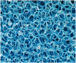
Figure 1. (a,b) Sketches showing the key components of the experimental set-up, including the positioning of the horizontal grid, the porous layer and the inner and outer boxes; (a) shows a sides view and (b) shows a plan view. Also shown are the coordinate directions $(x_1,x_2,x_3)$, and the vertical distance from the permeable boundary, denoted $\xi =H-x_3$. The permeable media used are shown in (c,d); 60 pores per inch (PPI) and 10 PPI foams are shown, respectively. Each permeable medium is shown at the same scale (a reference scale is provided in (d) which applies to both images).

Two different porous media were used for this study, in addition to a solid impermeable surface. The impermeable surface was formed by inserting a solid acrylic plate into the inner box at a depth $H\approx 4.2M$ below the grid's mean position (see figure 1a). A tight fit was ensured between the plate and the inner box by use of thin neoprene seals, set into the perimeter of the plate. The porous media were comprised of 2.5 cm thick sheets of reticulated polyether foam that were inserted into the inner box, parallel to the grid, and overlaid up to a total thickness of 10 cm. This ensured that the thickness of the permeable layers did not restrict the depth of flow penetration. The surface of the porous medium was also located at a depth $H\approx 4.2M$ below the grid's mean position.

Reticulated polyether foams have a regular structure comprising open cells that are pentagonal dodecahedra in shape (see, for example, Szycher Reference Szycher2012; Defonseka Reference Defonseka2019). During the manufacturing process the thin membranes that initially form the faces of each cell are removed, such that the foams consist of a network of interconnected thin filaments. Consequently, reticulated polyether foams are 97 % voids by volume (i.e. porosity of 97 %) (Szycher Reference Szycher2012; Defonseka Reference Defonseka2019). The size of cells formed can be carefully controlled during the manufacturing process, thus foams are available over a wide range of permeabilities. For this study two foams of different permeabilities were used, which are shown in figure 1(c,d). The geometry of these permeable media are ideal for studying the effects of permeability on wall turbulence as the high porosity and small filament thickness of the foams minimises the influence of the roughness of the interface between the porous layer and the fluid above. Consequently, reticulated polyether foams have also been used in previous studies investigating permeable boundaries (see, for example, Manes et al. Reference Manes, Poggi and Ridolfi2011; Mujal-Colilles, Dalziel & Bateman Reference Mujal-Colilles, Dalziel and Bateman2015). The absolute permeability, $K$, of each foam used is shown in table 1, which was determined using a constant head permeameter test (British Standards Institution 2010) in which the permeability was determined from measurements of the pressure drop across a sample at a given (constant) volume flow rate. Lower and upper bounds for the size of the dodecahedral cells, $l_{cell}$, present in each porous medium, are also shown in table 1, which were provided by the manufacturer (Reticel, private communication). Cell sizes were determined using the Visiocell method (see, for example, Mullens, Luyten & Zeschky Reference Mullens, Luyten and Zeschky2006, p. 236). Commercially, reticulated polyether foams are typically characterised by the mean number of pores present in a linear inch (PPI) of the permeable matrix; for this study 10 PPI and 60 PPI foams were used. We stress that this measure is poorly defined, since it is unclear whether in this context ‘pore’ refers to the dodecahedral cells of the foam or the component faces of the cells. Consequently, this measure is used here only in a descriptive context in order to facilitate identification of similar foams used in previous studies. To ensure the foams were fully saturated when in use, each foam was submerged in a beaker of tap water and placed in a vacuum chamber to reduce the ambient pressure to approximately $-0.9$ bar (gauge pressure), which deaerated the water and foam. The foams were thereafter kept submerged to prevent aeration of the foams.

Table 1. A summary of hydraulic conductivity, $k_p$, and absolute permeability, $K$, results obtained from permeability testing of the reticulated polyether foams. Lower and upper bounds of these estimates are shown in brackets. Also shown are lower and upper bounds for the size of the cells of the porous media, $l_{cell}$. Values of the permeability Reynolds number $Re_K$ used are also shown, which correspond to experiments conducted at the respective grid Reynolds numbers of $Re_G \equiv MSf/\nu \approx$ 2020, 4220, 5260, 6480 and 8100.

For each boundary considered, we report results from 5 sets of experiments in which the stroke $S$ was set to be either 2.5 cm or 3.0 cm and the frequency of the grid's oscillation $f$ was varied between 1.6 and 5.4 Hz. The corresponding grid Reynolds numbers for these five experiments were $Re_G \equiv MSf/\nu \approx$ 2020, 4220, 5260, 6480 and 8100. For each experimental condition, the experiments were repeated, under nominally identical conditions, a total of 5 times; this approach facilitates the use of ensemble averages to reduce scatter in the data. We note that we have also re-used measurements from previous experiments that investigated the interaction of oscillating-grid turbulence with an impermeable surface (McCorquodale & Munro Reference McCorquodale and Munro2018a), but we focus here on reporting new data that illustrate the effects of boundary permeability on the interaction.

2.2. Measurements and notation

In each experiment, two-dimensional two-component particle image velocimetry (PIV), applied to the vertical plane through the centre of the grid, as shown in figure 1(b), was used to acquire measurements of instantaneous fluid velocities in the region inside the inner box spanned by the grid and the permeable medium. The flow was seeded with neutrally buoyant tracer particles (Pliolite with diameter range $75\text {--}125\ \mathrm {\mu }\textrm {m}$), which were illuminated within a thin light sheet produced by a pulsed laser. Images of illuminated particles were recorded at 100 frames per second (at $1280\times 1024$ pixel resolution) using a high-speed digital camera aligned perpendicular to the plane of the light sheet. PIV calculations were performed using square interrogation windows of $13\times 13$ pixels, overlapped to achieve 8 pixel spacing between velocity vectors, resulting in a physical spacing between velocity vectors of approximately 0.16 cm. We note that the parameters used for the PIV were chosen to conform with the guidelines recommended by Keane & Adrian (Reference Keane and Adrian1990).

The velocity data were calculated and analysed relative to the right-handed coordinate system $(x_1,x_2,x_3)$; here, $x_3$ denotes vertical depth below the mid-height of the grid's oscillation, and $(x_{1},x_{2})$ are the horizontal coordinates relative to the centre of the grid (see figure 1). The corresponding velocity components are denoted $(u_1,u_2,u_3)$; the two components measured using the PIV set-up described above are $u_1(x_1,x_3,t)$ and $u_3(x_1,x_3,t)$, in the central plane at $x_2=0$. We also introduce the coordinate $\xi =H-x_{3}$ to denote vertical height above the permeable boundary (see figure 1a). This coordinate is used only for convenience when plotting and comparing data; we stress that all velocities (and derivatives of velocities) were calculated in terms of the right-handed coordinates $(x_1,x_2,x_3)$. Sufficiently far beneath the grid (see § 2.3), oscillating-grid turbulence (OGT) is statistically stationary and so the statistical properties of the flow in this region were analysed using time averages. We use the conventional Reynolds decomposition $u_i = U_i + u_i'$, where $u_i'(\boldsymbol {x},t)$ denote the fluctuating components and $U_i(\boldsymbol {x})=\overline {u_i}$ the time-averaged mean components (the overbar notation is used throughout to denote time averaging). In each experiment velocity data were captured for a period of 240 s; analysis of the data showed that the time-averaged mean and r.m.s. of fluctuating velocity components were converged to within approximately 5 % of their ultimate values over this time period (McCorquodale & Munro Reference McCorquodale and Munro2018a,Reference McCorquodale and Munrob).

Alongside measurement errors, the relatively slow convergence of the experimental data results in not-insignificant experimental uncertainty. However, we stress that the ensemble of 5 repeat tests for each experiment that we report provides an estimate of uncertainty within the data. In the analysis presented in §§ 3 and 4 the experimental uncertainty is indicated by error bars. (A single representative set of error bars is shown in each figure to prevent the plots from becoming cluttered.) These error bars illustrate that the uncertainty in the experimental measurements is small in the context of permeability effects that we identify.

Finally, we note that the estimates of uncertainty described above do not include the influence of sampling errors arising from the limited resolution of the PIV data. That is, within the region of the flow for which velocity measurements were obtained (i.e. for $x_3\gtrsim 2.5M$), the Kolmogorov length scale $\eta$ was estimated to be of the order $\eta \sim 0.05\ \textrm {cm}$, which is finer than the physical spacing between velocity vectors computed by the PIV calculations (approximately 0.16 cm). (The Kolmogorov length scale was estimated using the relation $\eta =\nu ^{3/4}\varepsilon ^{-1/4}$ under the assumption that, in OGT, $\varepsilon \approx 0.75 (\overline {u'^2_1})^{3/2}/\bar {\ell }$ for $x_3\gtrsim 2.5M$ (Kit, Strang & Fernando Reference Kit, Strang and Fernando1997).) Thus, the resolution used for PIV calculations was coarser than the smallest turbulent scales within the flow, such that velocity averaging occurred across interrogation windows and some turbulent fluctuations were unresolved. Consequently, the full energy content of the turbulent flow was not determined by the analysis. However, we stress that the range in scales of turbulent fluctuations that were under-resolved in the current analysis is very small in the context of the size of the integral scales of the turbulent flow (which are of the order 2 cm in size, see § 3). The implications of the limited resolution of the velocity measurements for the analysis presented in §§ 3 and 4 is discussed within these sections.

2.3. Description of the flow produced

Close to the oscillating grid, henceforth referred to as the ‘near-grid region’, jets form in the wake of the grid elements resulting in a flow field characterised by the presence of energetic, mesh-sized coherent vortex structures that interact and breakdown as they are advected away from the grid. This coherent flow structure breaks down within a distance of 2.5 mesh lengths from the grid (i.e. for $x_3 \lesssim 2.5M$) (see, for example, McCorquodale & Munro Reference McCorquodale and Munro2018b). Within the near-grid region the oscillation of the grid directly influences the structure of the flow on a time scale of the order $1/f$. However, under ideal conditions, the turbulent flow beyond this region, which we henceforth refer to as the ‘turbulent-diffusive region’, is statistically stationary, homogeneous and isotropic in planes parallel to the grid, with negligible mean flow (De Silva & Fernando Reference De Silva and Fernando1994). Moreover, velocity measurements in this region do not indicate the presence of periodic signatures relating to the grid forcing (McCorquodale & Munro Reference McCorquodale and Munro2017). The turbulence is, however, inhomogeneous in planes normal to the grid; the r.m.s. turbulent velocity components $u$ and $w$ (where $w\equiv (\overline {u'_3u'_3})^{1/2}$, $u\equiv (\overline {u'_1u'_1})^{1/2}$) decay with increasing distance normal to the grid. The presence of the impermeable plate or porous layer inserted above the base of the acrylic box also results in a boundary-affected region of the flow, which we define as the thin layer of height $\delta _{s}$ above the boundary over which the degree of isotropy $w/u$ departs from a value of 1 and decreases as the boundary is approached. McCorquodale & Munro (Reference McCorquodale and Munro2017) reported that with the current apparatus $\delta _{s}$ is of the order of the integral length scale of the turbulence when the boundary is impermeable. The results reported here for permeable media are consistent with this observation (see § 3.1).

Under the idealised conditions assumed to occur beyond the near-grid region of the flow, the steady form of the Reynolds stress transport equations may be written as

(2.1)\begin{align} 0= \underbrace{-\frac{\partial}{\partial x_{k}}\overline{u'_{i}u'_{j}u'_{k}}}_{T_{ij}} \underbrace{-\frac{1}{\rho} \left( \frac{\partial}{\partial x_{i}}\overline{p'u'_{j}} + \frac{\partial }{\partial x_{j}}\overline{p'u'_{i}} \right)}_{\varPi^d_{ij}} +\underbrace{\frac{1}{\rho}\overline{ p'\left( \frac{\partial u'_{j}}{\partial x_{i}} + \frac{\partial u'_{i}}{\partial x_{j}} \right) }}_{\varPi^s_{ij}} +\underbrace{\nu \frac{\partial^{2}\overline{u'_{i}u'_{j}}}{\partial x_{k}\partial x_{k}} }_{D_{ij}} \underbrace{-2\nu \overline{\frac{\partial u'_{i}}{\partial x_{k}} \frac{\partial u'_{j}}{\partial x_{k}}}}_{\varepsilon_{ij}}. \end{align}

The terms $T_{ij}$ and $\varPi ^d_{ij}$ denote, respectively, transport by velocity and pressure fluctuations; $\varPi ^s_{ij}$ is the inter-component energy redistribution due to the correlation between fluctuating strain and pressure fields; $D_{ij}$ and $\varepsilon _{ij}$ denote viscous diffusion and viscous dissipation. We stress that since the turbulence is approximately homogeneous on horizontal planes then $\overline {u'_{i}u'_{j}} \thickapprox 0$ for $i \neq j$. Hence, a comprehensive understanding of the flow follows from considering terms of the transport equations for the Reynolds stresses $\overline {u'_1u'_1}$, $\overline {u'_2u'_2}$ and $\overline {u'_3u'_3}$ (i.e. $u^2$, $v^2$ and $w^2$), and the transport equation for TKE, which is obtained from the trace of (2.1) noting that $\overline {u'_iu'_i}/2 = \overline {q'^2}$ denotes the TKE.

From (2.1) it follows that the TKE transport equation may be written as

(2.2)\begin{equation} 0= \underbrace{-\frac{1}{2}\frac{\partial}{\partial x_{k}}\overline{u'_{i}u'_{i}u'_{k}}}_{T_{ii}} \underbrace{-\frac{1}{\rho} \frac{\partial }{\partial x_{i}}\overline{p'u'_{i}} }_{\varPi^d_{ii}} +\underbrace{\frac{\nu}{2} \frac{\partial^{2}\overline{u'_{i}u'_{i}}}{\partial x_{k}\partial x_{k}} }_{D_{ii}} \underbrace{-\nu \overline{\frac{\partial u'_{i}}{\partial x_{k}} \frac{\partial u'_{i}}{\partial x_{k}}}}_{\varepsilon_{ii}}, \end{equation}

but by noting that turbulence is homogeneous in the $x_{1}\text {--}x_{2}$ plane, parallel to the grid, such that turbulence statistics only vary in the $x_{3}$ direction, the TKE budget can be simplified to

(2.3)\begin{equation} 0 ={-}\dfrac{\mathrm{d}}{\mathrm{d}x_{3}}\left(\dfrac{\overline{p'u_{3}'}}{\rho} + \overline{u_{3}'q'^2} + \nu \dfrac{\mathrm{d}}{\mathrm{d}x_{3}} \overline{q'^2} \right) +\varepsilon . \end{equation}

Outside the boundary-affected region the viscous transport term can be assumed to be negligible, since the transfer process is predominantly inertial in high Reynolds number flows, and thus in the turbulent-diffusive region the flow is governed by a balance of the viscous dissipation of TKE and the transport of TKE by velocity and pressure fluctuations.

By parametrising the leading-order terms of (2.3), Thompson & Turner (Reference Thompson and Turner1975) and Hopfinger & Toly (Reference Hopfinger and Toly1976) were able to obtain an expression describing the spatial decay of the r.m.s. velocity components $u$ and $w$ with increasing distance normal to the grid, valid within the turbulent-diffusive region. The resulting expression has since been validated empirically and flow in the turbulent-diffusive region is commonly described by the standard model

(2.4a)\begin{gather} u= C_{1} S f \left(\frac{x_{3}}{M^{1/2} S^{1/2}}\right)^{-\gamma}, \end{gather}

(2.4b)\begin{gather}w= C_{2} u, \end{gather}

with $\gamma \thickapprox 0.8\text {--}1.5$, $C_1 \thickapprox 0.2\text {--}0.5$ and $C_2 \thickapprox 1.1\text {--}1.4$ (Thompson & Turner Reference Thompson and Turner1975; Hopfinger & Toly Reference Hopfinger and Toly1976; McDougall Reference McDougall1979; Hopfinger & Linden Reference Hopfinger and Linden1982; Atkinson, Damiani & Harleman Reference Atkinson, Damiani and Harleman1987; Nokes Reference Nokes1988; De Silva & Fernando Reference De Silva and Fernando1994; Kit et al. Reference Kit, Strang and Fernando1997).

Simple expressions can also be obtained to describe how the time-averaged mean dynamic pressure, denoted $P$, should vary within the turbulent-diffusive and boundary-affected regions of the flow. That is, rearranging the steady mean-flow momentum equations, and omitting the body force term for gravitational acceleration since we concerned with the dynamic pressure, gives

(2.5)\begin{equation} \frac{\partial P}{\partial x_{i}} ={-}\rho U_{j}\frac{\partial U_{i}}{\partial x_{j}} -\rho\frac{\partial (\overline{u'_{i}u'_{j}})}{\partial x_{j}} + \mu \frac{\partial^2 U_{i}}{\partial x_{j} \partial x_{j}}, \end{equation}

where $\mu$ denotes dynamic viscosity. Under ideal conditions (i.e. negligible mean flow, with turbulence that is homogeneous in the $x_{1}\text {--}x_{2}$ plane, parallel to the grid), these equations simplify to

(2.6a,b)\begin{equation} \frac{\partial P}{\partial x_{3}} ={-}\rho \frac{\partial(\overline{u'_{3}u'_{3}})}{\partial x_{3}} ={-}\rho \frac{\partial w^2}{\partial x_{3}} \quad\text{and}\quad \frac{\partial P}{\partial x_{i}}=0, \quad i=1,2. \end{equation}

Hence, in light of (2.4), within the turbulent-diffusive region we expect the mean dynamic pressure to increase with depth beneath the grid, but at a rate that decays with increasing $x_3$.

In practice, minor differences in the flow produced by OGT apparatus are found to occur relative to the idealised flow described above. In particular, OGT apparatus are known to exhibit secondary circulations (see, for example, McKenna & McGillis Reference McKenna and McGillis2004), which give rise to small mean flow velocities within the turbulent-diffusive and boundary-affected regions of the flow. We stress that the OGT apparatus used in this study has been specifically designed to conform with experimental conditions that have been found to minimise the magnitude of the mean-flow velocities within the turbulent-diffusive and boundary-affected regions of the flow (Hopfinger & Toly Reference Hopfinger and Toly1976; McDougall Reference McDougall1979; Fernando & De Silva Reference Fernando and De Silva1993; McCorquodale & Munro Reference McCorquodale and Munro2018b). Consequently, previous studies using the same apparatus (McCorquodale & Munro Reference McCorquodale and Munro2017, Reference McCorquodale and Munro2018b) indicate that within the turbulent-diffusive and boundary-affected region of the flow the turbulent velocity components are of comparable or greater magnitude than mean-flow velocity components. Moreover, having acquired measurements of terms in the transport equation for TKE representing the transport and production due to the mean flow, McCorquodale & Munro (Reference McCorquodale and Munro2017) concluded that although the presence of a mean flow indicates the presence of mean shear in the boundary-affected region – such that the turbulence is not strictly zero mean shear – the levels are sufficiently small in magnitude to allow meaningful comparisons to be made with zero-mean-shear conditions. McCorquodale & Munro (Reference McCorquodale and Munro2017, Reference McCorquodale and Munro2018b) also showed that anisotropic regions exist adjacent to the tank sidewalls, but that the flow in the turbulent-diffusive region is approximately homogeneous on the $x_{1}\text {--}x_{2}$ plane, parallel to the grid, over a central region of the inner tank (i.e. for $\vert x_1/L \vert \leq 1/2$). Hence, throughout this paper, our attention is focused on the central region $\vert x_1/L \vert \leq 1/2$ and the sidewall anisotropic regions are ignored in the calculation of turbulent statistics. The notation $\langle \cdot \rangle _1$ is henceforth used to denote quantities that have been spatially averaged, in the $x_1$ direction, over this region.

For each experiment reported here, data describing the statistical structure of the mean and turbulent components of the flow above the boundary-affected region were in good agreement with the above description of the flow. (We note that representative results describing the structure of the flow produced by the apparatus have also been reported previously by McCorquodale & Munro (Reference McCorquodale and Munro2017) and McCorquodale & Munro (Reference McCorquodale and Munro2018b).) Consequently, here we focus on reporting results within the boundary-affected region of the flow, which, recall, we define as the thin layer of height $\delta _{s}$ above the permeable boundary over which the degree of isotropy $w/u$ departs from a value of 1 and decreases as the boundary is approached.

2.4. Permeability Reynolds number

Throughout this paper, the effects of boundary permeability are characterised using the permeability Reynolds number $Re_{K}$, which is a measure of the inhibiting effects of viscous forces at a permeable boundary. Physically, $Re_{K}$ can be interpreted as the ratio of the typical pore size in a permeable matrix, which scales with the square root of the absolute permeability $\sqrt {K}$ (see for example Katz & Thompson Reference Katz and Thompson1986), to the typical viscous sublayer thickness $\delta _v$ over the surface of the elements that constitute the permeable medium. (The viscous sublayer at the surface of a porous medium retains the same interpretation as the viscous sublayer at an impermeable boundary; the viscous sublayer is the region of flow adjacent to the surface(s) of an impermeable boundary or a porous medium in which viscous stresses predominate over turbulent stresses.) In a channel flow, the viscous sublayer scales with $\nu /u_*$, such that (Breugem et al. Reference Breugem, Boersma and Uittenbogaard2006)

(2.7)\begin{equation} Re_{K}\equiv \frac{u_* \sqrt{K}}{\nu}, \end{equation}

where $u_*$ denotes the friction velocity.

However, an alternative expression for the viscous sublayer thickness is required for the current problem in which zero-mean-shear turbulence interacts with a boundary ($u_*$ is undefined in the current flow). In studying the interaction of an initially isotropic turbulent flow with an impermeable surface that moves at the free-stream velocity of the turbulent flow, such that there is zero mean shear in the boundary-affected region of the flow, Hunt & Graham (Reference Hunt and Graham1978) proposed that the viscous sublayer thickness $\delta _v$ over the impermeable boundary scaled as

(2.8)\begin{equation} \delta_v\propto [\nu\ell/u_{\delta}]^{1/2}, \end{equation}

where $\ell$ denotes the integral length scale of the turbulence outside the boundary-affected region and $u_\delta =(\overline {u'_1u'_1})^{1/2}$ at $\xi =\delta _s$. Since these terms are defined at the edge of the boundary-affected region, these definitions preclude any effects on the flow relating to the modifying effects of the boundary. In addition, in turbulence that is otherwise isotropic outside the boundary-affected region $\overline {u'_1u'_1} = \overline {u'_2u'_2} = \overline {u'_3u'_3}$ so that each velocity component can be used interchangeably for this characteristic value of $u{_\delta }$. Hunt (Reference Hunt1984) subsequently asserted the validity of this expression for the flow considered in this study, in which statistically steady turbulence interacts with a surface in the absence of mean shear. That is, in the current flow, $\delta _v$ is estimated to be smaller than the integral length scale $\ell$, which scales with the thickness of the boundary-affected region, by a factor equal to the square root of the turbulent Reynolds number, i.e. $\delta _v/\delta _s \propto \delta _v/\ell \propto Re^{-1/2}$ where $Re\equiv u_{\delta }\ell /\nu$. Equation (2.8) gives rise to a permeability Reynolds number defined as

(2.9)\begin{equation} Re_{K}\equiv \sqrt{\frac{u_{\delta}K}{\nu\ell}}. \end{equation}

The values of $Re_{K}$ for each experimental condition, evaluated using (2.9), are shown in table 1.

We note that although previous studies using OGT have reported measurements of the viscous sublayer thickness of the order given by (2.8) (Brumley & Jirka Reference Brumley and Jirka1987; Kit et al. Reference Kit, Strang and Fernando1997), here, the corresponding measurements did not obey the implied $Re^{-1/2}$ scaling. That is, (2.8) predicts values of $\delta _v$ of the correct order of magnitude, but the measurements of $\delta _v$ did not exhibit any consistent Reynolds number scaling. We attribute this result to the small Reynolds number range considered and uncertainty in the methods used to define the edge of the viscous sublayer.

3.1. Thickness of the boundary-affected region

In § 2 we defined the boundary-affected region as a thin layer, of thickness $\delta _s$, directly above the boundary over which the degree of isotropy $\langle w \rangle _1/\langle u \rangle _1$ departs from its value of approximately 1 away from the boundary, and decreases as the boundary is approached. At this point it is instructive to define a reference value $\ell _0$ of the (time-averaged) integral length scale $\bar {\ell }$; previous research indicates that $\delta _s$ scales with the integral length scale of the turbulence (Perot & Moin Reference Perot and Moin1995).

Estimates for the integral length scales were obtained from the velocity measurements by computation of autocorrelation coefficients, using the approach previously described by Kit et al. (Reference Kit, Strang and Fernando1997) and McCorquodale & Munro (Reference McCorquodale and Munro2017). That is, the integral length scale $\ell$ is defined as the integral of the autocorrelation function of $u'_1(x_1,x_3,t)$, over the spatial lag up to which the autocorrelation function first crosses zero; time-averaged integral length scales are denoted $\bar {\ell }$. The computed values of $\bar {\ell }$ are shown in figure 2(a), plotted against height, $\xi$, above the boundary. Figure 2(a) shows that $\bar {\ell }$ exhibits a notable degree of scatter, but for $\xi \gtrsim 3\ \text {cm}$ the data are relatively constant, taking values typically between 2 and 2.3 cm. For heights $\xi < 3\ \mathrm {cm}$ the values of $\bar {\ell }$ increase slightly, before rapidly reducing at $\xi \thickapprox 0.75\ \mathrm {cm}$. Figure 2(a) also shows that slightly larger values of $\bar {\ell }$ are obtained for experiments conducted at the larger values of $Re_G$ considered. No link between the values of $\bar {\ell }$ and permeability Reynolds number $Re_K$ was identified. In order to facilitate comparison with previous work (McCorquodale & Munro Reference McCorquodale and Munro2017, Reference McCorquodale and Munro2018a), we define the reference integral length scale $\ell _{0}$ to be the peak value attained by $\bar {\ell }$ in the near-boundary region.

Figure 2. (a) Computed values of the time-averaged integral length scale, $\bar {\ell }$, plotted against height $\xi$. (b) Measurements of the degree of isotropy $\langle w \rangle _1/\langle u \rangle _1$, plotted against normalised height $\xi /\ell _0$. In both plots a single data set is shown for each experimental condition reported in table 1, which is an average of the measurements obtained across the $n=5$ repeats conducted for each condition. In (a), data obtained at different $Re_G$ are shown separately by line colour (see legend), whilst the type of boundary in use is shown by the line type; ‘–’, ‘- -’ and ‘- $\cdot$ -’ denote an impermeable surface, 60 PPI porous layer and 10 PPI porous layer, respectively. In (b), data at different $Re_K$ are shown separately, irrespective of $Re_G$ (see legend). Also shown are representative error bars, corresponding to the standard error across the $n=5$ repeats; error bars are shown for the cases $Re_G\approx 8100$ and $Re_K\approx 0.30$ in (a,b) respectively.

Turning now to estimates of the thickness of the boundary-affected region, measured values of the degree of isotropy $\langle w \rangle _1 / \langle u \rangle _1$ are shown in figure 2(b), plotted against scaled height $\xi /\ell _0$. Figure 2(b) shows a rapid increase in anisotropy occurs at $\xi /\ell _{0} \thickapprox 1$ as the boundary is approached, departing from the far-field trend $\langle w \rangle _1 / \langle u \rangle _1\approx 1$. No link has been identified with either $Re_G$ or $Re_K$ and the point at which this departure from the far-field trend occurs. We therefore conclude that the boundary-affected region extends up to $\delta _s/\ell _{0} \thickapprox \xi /\ell _{0}\thickapprox 1$ across the entire $Re_{K}$ range considered.

However, we note that the data in figure 2(b) show the degree of anisotropy over the region $\xi /\ell _0\lesssim 0.5$ is affected by the boundary permeability $Re_K$. That is, increasing $Re_K$ reduces the observed anisotropy. In figure 2(b), results for $Re_{K}\lesssim 0.2$ collapse, to within experimental uncertainty, onto the data obtained for $Re_{K}\thickapprox 0$, but there is a distinct departure from this trend for $Re_{K}\gtrsim 0.2$. This indicates that for $Re_{K}\lesssim 0.2$ the boundary is effectively impermeable and the no-penetration and viscous boundary conditions are, at least approximately, enforced. In contrast, for $Re_{K}\gtrsim 0.2$ boundary permeability has a contributing effect to the turbulence structure in the boundary-affected region.

3.2. Root-mean-square velocity data and turbulent kinetic energy

Here, we consider the r.m.s. of fluctuating velocity components in more detail in order to explain how boundary permeability influences the degree of isotropy within the boundary-affected region. The effect of the boundary on the r.m.s. turbulent velocity components is shown in figure 3(a,b). The data have been normalised using values of the r.m.s. turbulent velocity components that we would expect in the absence of the boundary. That is, values of $u$ and $w$ that would be expected in the absence of the boundary, which we denote $u_0$ and $w_0$, were determined by applying a best fit of the form given by (2.4) to measurements of $\langle u \rangle _1$ and $\langle w \rangle _1$ in the turbulent-diffusive region of the flow (i.e. $\xi >\ell _0$) and extrapolating the best fit to the boundary-affected region of the flow (i.e. $\xi <\ell _0$). Using this approach, estimates of $u_0$ and $w_0$ were evaluated for each vertical location within the boundary-affected region of the flow at which measurements of $\langle u \rangle _1$ and $\langle w \rangle _1$ were obtained. A similar procedure has also been used to obtain reference values for other parameters reported in this section.

Figure 3. Plots showing the scaled r.m.s. of fluctuating velocity components (a) $\langle w \rangle _{1}/w_{0}$ and (b) $\langle u \rangle _{1}/u_{0}$. In each plot a single data set is shown for each experimental condition reported in table 1, which is an average of the measurements obtained across the $n=5$ repeats conducted for each condition. The data at different $Re_K$ are shown separately, irrespective of $Re_G$. Also shown are representative error bars for the case $Re_K\approx 0.3$, corresponding to the standard error across the $n=5$ repeats.

Figure 3(a) shows that the boundary-normal component $w$ is monotonically reduced by the presence of the boundary. For $Re_K\lesssim 0.2$ the observed reduction in $w$ is in quantitative agreement with results from previous studies investigating the interaction of zero-mean-shear turbulence with an impermeable boundary (Thomas & Hancock Reference Thomas and Hancock1977; Hunt & Graham Reference Hunt and Graham1978; Hannoun, Fernando & List Reference Hannoun, Fernando and List1988; Aronson, Johansson & Löfdahl Reference Aronson, Johansson and Löfdahl1997). However, figure 3(a) also shows that the magnitude of $w/w_0$ over $\xi /\ell _0\lesssim 0.5$ is slightly greater for experiments conducted at $Re_K>0.2$ and suggests the magnitude increases with increasing $Re_K$. Although a small effect, these data indicate that for $Re_K\gtrsim 0.2$ the boundary permeability begins to inhibit the kinematic blocking condition that is otherwise enforced when $Re_K=0$.

A more pronounced $Re_K$ effect is evident in the measurements of the horizontal (i.e. boundary-tangential) component ($u$), shown in figure 3(b). The results indicate that for $Re_K\lesssim 0.2$ the boundary acts to increase $u$ within the boundary-affected region, relative to the far-field trend, except in a thin viscous region immediately adjacent to the boundary. These data are in agreement with results from previous studies investigating the interaction of OGT, and random jet arrays, with an impermeable boundary (Brumley & Jirka Reference Brumley and Jirka1987; Hannoun et al. Reference Hannoun, Fernando and List1988; McCorquodale & Munro Reference McCorquodale and Munro2017; Johnson & Cowen Reference Johnson and Cowen2018). Notably, however, figure 3(b) shows that the amplification of $u/u_0$ within the boundary-affected region ($\xi /\ell _0\lesssim 1$) is significantly inhibited with increasing $Re_K$, for $Re_K\gtrsim 0.2$.

Given this relative increase in $w$ and relative decrease in $u$, within the boundary-affected region, with increasing $Re_K$, a logical explanation would be that changes in intercomponent energy transfer between the velocity components occur as the boundary permeability increases. Recall, intercomponent energy transfer is described by the term $\varPi ^s_{ij}$ in (2.1). Indeed, in § 4 we argue that this is one of the contributing mechanisms. However, the changes in the velocity components described above also correspond to changes in turbulent kinetic energy within the boundary-affected region.

Measurements of TKE, here defined as $\overline {q'^2}=\overline {u'_{i}u'_{i}}/2 \approx (2\overline {u'_{1}u'_{1}} +\overline {u'_{3}u'_{3}})/2$ (where $v\thickapprox u$ has been assumed), are shown in figure 4(a). In accordance with the results of the r.m.s. turbulent velocity components, figure 4(a) shows $\langle \overline {q'^2} \rangle _{1}$ scaled by $\overline {q'^2_0}$, which denotes the values of $\langle \overline {q'^2} \rangle _{1}$ that would be expected in the absence of the boundary, obtained by extrapolating a best fit applied to the data above the boundary-affected region. Figure 4(a) shows that when $Re_{K}\lesssim 0.2$ (i.e. the boundary is effectively impermeable) the results exhibit $\langle \overline {q'^2} \rangle _{1}/\overline {q'^2_0}>1$ within the boundary-affected region, in accordance with previous results at an impermeable boundary (Hannoun et al. Reference Hannoun, Fernando and List1988; McCorquodale & Munro Reference McCorquodale and Munro2017; Johnson & Cowen Reference Johnson and Cowen2018). This indicates that for $Re_K\lesssim 0.2$ there is an increase in turbulent kinetic energy within the boundary-affected region ($\xi /\ell _0\lesssim 1$), relative to expected values in the absence of the boundary. However, figure 4(a) shows significant reductions in $\langle \overline {q'^2} \rangle _{1}/\overline {q'^2_0}$ occur within the boundary-affected region as $Re_K$ is increased. Moreover, for $Re_K\approx 0.38$ figure 4(a) shows that $\langle \overline {q'^2} \rangle _{1}/\overline {q'^2_0}<1$ when $\xi /\ell _0<1$, indicating that in this case there is no increase in turbulent kinetic energy within the boundary-affected region, relative to expected values in the absence of the boundary. This reduction in TKE within the boundary-affected region (relative to an impermeable boundary) indicates that the changes in $u/u_0$ and $w/w_0$ described above cannot be explained only by changes in intercomponent energy transfer. Instead, the results can be explained using measurements of the TKE flux.

Figure 4. Measurements of (a) TKE $\langle \overline {q'^2} \rangle _1$, and (b) vertical flux of TKE, $\langle \overline {u'_{3}q'^2} \rangle _1$. Here, $\langle \overline {q'^2} \rangle _1$ and $\langle \overline {u'_{3}q'^2} \rangle _1$ have been normalised by the values expected in the absence of the boundary, denoted $\overline {q'^2_0}$ and $(\overline {u_3'q'^{2}})_0$ respectively. In both plots a single data set is shown for each experimental condition reported in table 1, which is an average of the measurements obtained across the $n=5$ repeats conducted for each condition. The data at different $Re_K$ are shown separately, irrespective of $Re_G$. Also shown are representative error bars for the case $Re_K\approx 0.3$, corresponding to the standard error across the $n=5$ repeats.

A TKE flux exists throughout the flow due to the vertically inhomogeneous nature of the flow produced by OGT, whereby the magnitude of turbulent fluctuations decays with distance beneath the grid resulting in a flux of TKE vertically downwards and away from the grid. In § 2.3 we emphasised that the transport of TKE by velocity fluctuations $T_{ii}$ is a key process in determining the statistical structure of the flow in zero-mean-shear turbulence; the TKE transport equation for this flow is $0=T_{ii}+\varPi ^d_{ii}+D_{ii}+\varepsilon _{ii}$, where $T_{ii}=-\mathrm {d}(\overline {u'_3q'^2})/\mathrm {d}x_3$. Measurements of the vertical flux of TKE, $\langle \overline {u'_{3}q'^2} \rangle _1$, are shown in figure 4(b). As before, the data have been scaled by their expected trend in the absence of the boundary, denoted $(\overline {u_3'q'^{2}})_0$, again obtained from a best fit applied to the data above the boundary-affected region. Previous studies of OGT interacting with an impermeable boundary reported a reduction in the TKE flux within the boundary-affected region ($\xi /\ell _0\lesssim 1$) relative to the far field (Hannoun et al. Reference Hannoun, Fernando and List1988; McCorquodale & Munro Reference McCorquodale and Munro2017) as a result of the kinematic blocking effect of the boundary. In terms of the TKE transport equation, this observation corresponds to an increase in the transport of TKE by velocity fluctuations $T_{ii}$ within the boundary-affected region, which is offset by a reduction in transport of TKE by pressure fluctuations $\varPi ^{d}_{ii}$; within the boundary-affected region, values of $\varepsilon _{ii}$ and $D_{ii}$ have been reported to be approximately constant except within the viscous sublayer (McCorquodale & Munro Reference McCorquodale and Munro2017).

For $Re_{K}\lesssim 0.2$ the data in figure 4(b) are consistent with the trend previously reported for the case of an impermeable boundary and reveal that for $\xi /\ell _{0}\lesssim 0.5$ the direction of energy flux is reversed (i.e. $\langle \overline {u'_{3}q'^2} \rangle _1/(\overline {u_3'q'^{2}})_0 <0$), such that there is a small flux of energy away from the boundary. The result of this blocking of the TKE flux within the boundary-affected region is an increase in TKE (Hannoun et al. Reference Hannoun, Fernando and List1988; McCorquodale & Munro Reference McCorquodale and Munro2017), as shown in figure 4(a), since additional energy that would otherwise propagate past the boundary (in its absence) is trapped in the boundary-affected region. Thus, this effect gives rise to an increase in the boundary-tangential velocity components relative to expected values in the absence of the boundary (McCorquodale & Munro Reference McCorquodale and Munro2017), as shown in figure 3(b). We note that McCorquodale & Munro (Reference McCorquodale and Munro2018a) also proposed that, for $Re_K=0$, a weak net intercomponent energy transfer from $w^2$ to $u^2$ occurs over the region $0.3\lesssim \xi /\ell _0\lesssim 0.6$; this is consistent with the reversed direction of TKE flux shown in figure 4(b) over this region, and also contributes to observed values of $u/u_0>1$.

At a permeable boundary (i.e. for $Re_{K}\gtrsim 0.2$) the data in figure 4(b) indicate that the vertical energy flux does not reduce by as much within the boundary-affected region ($\xi /\ell _0<1$) relative to experiments at an effectively impermeable boundary ($Re_K\lesssim 0.2$). This trend indicates that the amplification of $T_{ii}$ within the boundary-affected region ($\xi /\ell _0\lesssim 1$) is inhibited with increasing $Re_K$, for $Re_K \gtrsim 0.2$. Most importantly, these data show that as the boundary is approached the TKE flux remains positive and so is oriented into the porous medium. This increase in energy flux is attributed to a reduction in the blocking effect of the boundary (consistent with figure 3a) which enables a weak flux of energy into the permeable medium when $Re_{K}\gtrsim 0.2$.

To better understand the vertical flux of TKE into the boundary-affected region we have decomposed $\langle \overline {u'_{3}q'^2} \rangle _1$ into its components $\langle \overline {u'_3u'^2_1}\rangle _1$, $\langle \overline {u'^3_3}\rangle _1$, which are shown in figure 5 against scaled height $\xi /\ell _0$.

Figure 5. Measurements of the components of the TKE flux (a) $\langle \overline {u'^3_{3}} \rangle _{1}$ and (b) $\langle \overline {u'^2_{1}u'_{3}} \rangle _{1}$, plotted against scaled height $\xi /\ell _0$. Each component has been normalised by the values for the total TKE flux expected in the absence of the boundary denoted $( \overline { u'_3 q'^2} )_0$. In both plots a single data set is shown for each experimental condition reported in table 1, which is an average of the measurements obtained across the $n=5$ repeats conducted for each condition. The data at different $Re_K$ are shown separately, irrespective of $Re_G$. Also shown are representative error bars for the case $Re_K\approx 0.3$, corresponding to the standard error across the $n=5$ repeats.

The vertical flux of $w^2$ is shown in figure 5(a), and is positive far from the boundary, which indicates a flux of energy away from the grid transported by turbulent fluctuations. As the boundary is approached we observe a gradual reduction in $\langle \overline {u'^3_{3}} \rangle _{1}/( \overline {u'_3 q'^2} )_0$ as a result of the blocking effect of the boundary. This trend appears to hold across the entire $Re_K$ range considered here, which is consistent with the results shown in figure 3(a) in which we observed that only very small increases in $w/w_0$ occurred as $Re_K$ increased.

The vertical flux of $u^2$ is shown in figure 5(b), and is also positive far from the boundary, indicating a flux of energy away from the grid. When $Re_K\lesssim 0.2$, $\langle \overline {u_{3}'u_{1}'^2} \rangle _{1}$ decreases on approach to the boundary, reaching approximately 0 at $\xi /\ell _0\thickapprox 0.6$. This trend can be attributed to the blocking effect of the boundary on the vertical TKE flux, which in isolation would act to give rise to constant values of $u$ within the boundary-affected region and correspondingly zero net vertical energy flux. For $\xi /\ell _0\lesssim 0.6$ the vertical flux of $u^2$ is small but becomes negative indicating that there is a small net flux of $u^2$ away from the boundary, which is associated with a net intercomponent energy transfer from $w^2$ to $u^2$ as fluid elements are blocked by the surface (McCorquodale & Munro Reference McCorquodale and Munro2018a). This trend continues until $\xi /\ell _0\thickapprox 0.3$, at which point $\langle \overline {u_{3}'u_{1}'^2} \rangle _{1}$ tends to zero as a result of viscous dissipative effects that are prevalent over the viscous sublayer (McCorquodale & Munro Reference McCorquodale and Munro2017). (We note that the viscous sublayer (in which significant dissipation of TKE occurs) has thickness of approximately 0.2 to 0.3$\ell _0$ (see figure 4a).) The negative values of $\langle \overline {u_{3}'u_{1}'^2} \rangle _{1}$ for $\xi /\ell _0\lesssim 0.6$ are responsible for the small negative values of $\overline {u'_3q'^2}$ observed over the region $\xi /\ell _0\lesssim 0.5$ in figure 4(b).

When $Re_K\gtrsim 0.2$, results shown in figure 5(b) show that $\langle \overline {u_{3}'u_{1}'^2} \rangle _{1}$ is not reduced by as much within the boundary-affected region and, at the largest $Re_K$, retains a positive value throughout, indicating that there is a weak net flux of $u^2$ into the porous medium. This result indicates that there is reduction in the blocking of the far-field energy flux as $Re_K$ increases and is consistent with the observed reduction in $u/u_{0}$ when $Re_K\gtrsim 0.2$ (figure 3c).

To summarise, results of the TKE and vertical flux of TKE indicate that a contributing factor to the reported reduction in $u/u_{0}$ as $Re_{K}$ increases (see figure 3b) is a reduction in the blocking effect of the boundary on the vertical TKE flux, giving rise to a net flux of $u^2$ into the porous medium when $Re_K\gtrsim 0.2$. This reduction in the blocking effect of the boundary on the TKE flux gives rise to the reduction in TKE within the boundary-affected region, as shown in figure 4(a), as energy is no longer trapped in the boundary-affected region. Note, however, that although the kinematic blocking condition is inhibited for $Re_K\gtrsim 0.2$, viscous dissipation is still significant close to the surface.

Further insight into the effects of boundary permeability can be derived by considering the time-averaged mean dynamic pressure, denoted $P$. To estimate the vertical mean-pressure gradient, $\partial P/\partial x_3$, in the boundary-affected region we used the measured velocity data to estimate the right-hand side of (2.5) (for $i=3$). The analysis showed that contributions to the right-hand side of (2.5) from the mean flow components (advection and dissipation) were in general small, and so in this case the mean dynamic pressure gradient can be reasonably approximated using (2.6a,b). Measurements of $- \partial w^2 / \partial x_3\approx \partial P/ \partial x_3$ are shown in figure 6. In figure 6 measurements of $\partial w^2/\partial x_3$ have been normalised using the integral length scale $\ell _0$ and the expected value of the r.m.s. of fluctuating velocity components at the edge of the boundary-affected region $u_{\delta ,0}$. Note that at the edge of the boundary-affected region $w/u\approx 1$ such that $u_{\delta ,0}$ and $w_{\delta ,0}$ are approximately equal and these values can be used interchangeably.

Figure 6. Measurements of $\partial w^2/\partial x_3$ plotted against scaled height $\xi /\ell _0$. A single data set is shown for each experimental condition reported in table 1, which is an average of the measurements obtained across the $n=5$ repeats conducted for each condition. The data at different $Re_K$ are shown separately, irrespective of $Re_G$. Also shown are representative error bars for the case $Re_K\approx 0.3$, corresponding to the standard error across the $n=5$ repeats.

The data in figure 6 indicate that within the boundary-affected region $\partial w^2/\partial x_3$ increases in magnitude (and is negative in sign) as the boundary is approached, such that (according to (2.6a,b)) there is an increase in the mean dynamic pressure gradient. Consequently, as the fluid approaches the boundary it undergoes an increase in mean dynamic pressure at the expense of the TKE (see, for example, Hunt & Graham Reference Hunt and Graham1978). Hunt & Graham (Reference Hunt and Graham1978) predicted that for otherwise spatially homogeneous and isotropic turbulence interacting with an impermeable boundary this effect leads to a reduction in TKE in the boundary-affected region. However, the data reported in § 3.2 show that the same effect does not hold here when the turbulence interacts with an effectively impermeable boundary (i.e. $Re_K\lesssim 0.2$), due to inhomogeneity in the $x_{3}$ direction. That is, the blocking effect of an impermeable boundary on the vertical energy flux results in additional energy contained within the boundary-affected region, relative to the same region in the absence of the boundary (McCorquodale & Munro Reference McCorquodale and Munro2017). As a consequence, in the boundary-affected region we observe an increase in both TKE and mean dynamic pressure.

However, the data in figure 6 indicate that, as $Re_K$ increases, there is a reduction in the magnitude of $\partial w^2/\partial x_3$ and thus the degree by which the mean dynamic pressure gradient increases within the boundary-affected region diminishes. The corresponding reduction in mean dynamic pressure (relative to an impermeable boundary) indicates there is a reduction in the blocking of turbulent motions by the boundary as $Re_K$ increases, consistent with the previous results. This interpretation of the velocity measurements has an important implication. If there is a reduction in blocking of turbulent motions by the boundary this must be as a result of transportation of turbulent energy into the boundary; in other words, there is a reduction in the formation of high-pressure stagnation events as fluid elements impinge onto the boundary (so-called ‘splats’). Crucially, it is thought that the imbalance between splats and antisplats (fluid elements ejecting away from the boundary as a result of high-pressure collisions between fluid parcels) is central to intercomponent energy transfer. Consequently, a reduction in the formation of high-pressure splats as $Re_K$ increases is thought to inhibit intercomponent energy transfer and also contribute to the reduction in the observed values of $\langle u \rangle _{1}/u_{0}$, shown in figure 3(b), as $Re_K$ increases. This effect is investigated in more detail in § 4.

4.1. Criteria for isolating splats and antisplats

It is instructive to revisit the criterion used by McCorquodale & Munro (Reference McCorquodale and Munro2018a) to identify splats and antisplats. Splat events moving towards the boundary ($u'_3>0$) yield negative values of the vertical strain rate $\partial u'_3/\partial x_3$ and antisplat events moving away from the boundary ($u'_3<0$) yield positive values of the vertical strain rate $\partial u'_3/\partial x_3$ (Perot & Moin Reference Perot and Moin1995; Magnaudet Reference Magnaudet2003; Bodart et al. Reference Bodart, Cazalbou and Joly2010). However, fluid elements that exhibit these statistical characteristics exist throughout the entire flow, as a consequence of the random structure of a turbulent flow. On the other hand, the blocking associated with the formation of splats and antisplats is expected to give rise to more strongly decelerating flow than observed in the bulk interior of the flow. McCorquodale & Munro (Reference McCorquodale and Munro2018a) proposed that splats and antisplats may be isolated from the background flow by use of quadrant analysis on measurements of $u'_3$ and $\partial u'_3/\partial x_3$, and by further applying a threshold or critical value on the magnitude of the vertical strain rate $\partial u'_3/\partial x_3$, defined in comparison to a reference value of strain rate given by $w/\bar {\ell }_w$ evaluated at the corresponding $x_3$. The reference strain rate was devised from an order of magnitude analysis (Bodart et al. Reference Bodart, Cazalbou and Joly2010; McCorquodale & Munro Reference McCorquodale and Munro2018a); when a packet of size $\ell$ meets an impermeable surface with velocity $u'_3$, the vertical strain rate can be estimated as $u'_3/\ell$. For a given point within the boundary-affected region, the average velocity and size of a fluid packet is given by $w$ and $\bar {\ell }_w$, where $\bar {\ell }_w$ denotes the time-averaged transverse integral length scale of the boundary-normal velocity component $u'_3$, thus giving an average reference strain rate of $w/\bar {\ell }_w$.

By analysing the magnitude of vertical strain rate both in the boundary-affected region and bulk interior of the flow, McCorquodale & Munro (Reference McCorquodale and Munro2018a) found the condition $\vert (\bar {\ell }_w/w)\partial u'_3/\partial x_3 \vert >6$ was sufficient to isolate splats and antisplats from background fluctuations. That is, the probability that the magnitude of the instantaneous vertical strain rate exceeds $6w/\bar {\ell }_w$ was found to be negligible outside the boundary-affected region (see figure 7), and thus strain rates that exceed this value within the boundary-affected region were thought to correspond to fluid elements that exhibit strongly decelerating flow in response to the blocking effect of a surface.

Figure 7. Measurements of the probability that the normalised strain rate $(\bar {\ell }_w/w)\partial u'_3/\partial x_3$ surpasses a given constant $\phi _T$ (the values of $\phi _T$ are shown in each plot). Data are separated into quadrants according to the sign of $u'_3$ and $\partial u'_3/\partial x_3$, as described by (4.1); (a) $Q_2$, (b) $Q_1$, (c) $Q_3$ and (d) $Q_4$. In each plot a single data set is shown for each experimental condition reported in table 1, which is an average of the measurements obtained across the $n=5$ repeats conducted for each condition. The data at different $Re_K$ are shown separately, irrespective of $Re_G$. Also shown are representative error bars for the case $Re_K\approx 0.3$, corresponding to the standard error across the $n=5$ repeats.

To investigate how boundary permeability influences splat and antisplat formation we consider the probability of events that exhibit characteristics expected of splats and antisplats. That is, we split velocity measurements into 4 quadrants based upon the sign of $u'_3$ and $\partial u'_3/\partial x_3$ and calculate

(4.1a)\begin{gather} \text{Quadrant 1}\ (Q_1): {P}_{Q_1}\equiv\left\langle{P}\left( \frac{\bar{\ell}_w}{w} \frac{\partial u'_3}{\partial x_3} >\phi_{T} \cap u'_3>0\right)\right\rangle_1, \end{gather}

(4.1b)\begin{gather}\text{Quadrant 2}\ (Q_2): {P}_{Q_2}\equiv\left\langle{P}\left( \frac{\bar{\ell}_w}{w} \frac{\partial u'_3}{\partial x_3} >\phi_{T} \cap u'_3<0\right)\right\rangle_1, \end{gather}

(4.1c)\begin{gather}\text{Quadrant 3}\ (Q_3): {P}_{Q_3}\equiv\left\langle{P}\left( \frac{\bar{\ell}_w}{w} \frac{\partial u'_3}{\partial x_3} <{-}\phi_{T} \cap u'_3<0\right)\right\rangle_1, \end{gather}

(4.1d)\begin{gather}\text{Quadrant 4}\ (Q_4): {P}_{Q_4}\equiv\left\langle{P}\left( \frac{\bar{\ell}_w}{w} \frac{\partial u'_3}{\partial x_3} <{-}\phi_{T} \cap u'_3>0\right)\right\rangle_1, \end{gather}

as a function of $\xi /\ell _0$, where $P(A\cap B)$ denotes the probability of $A$ and $B$ and $\phi _T$ denotes a (positive) constant. When $\phi _T=0$ we consider the probabilities of each quadrant $P_{Q_i}$ based upon every measurement of the flow field (i.e. $P_{Q_1}+P_{Q_2}+P_{Q_3}+P_{Q_4}=1$ when $\phi _T=0$). When $\phi _T>0$ the evaluated probabilities associated with each quadrant decrease because those events that exhibit $\vert (\bar {\ell }_w/w)\partial u'_3/\partial x_3\vert < \phi _T$ are excluded from the analysis. The value of $\phi _T$ used to isolate splats (${Q_4}$) and antisplats (${Q_2}$) from the background fluctuations, identified previously by McCorquodale & Munro (Reference McCorquodale and Munro2018a), is $\phi _T=6$. In the following, a comparison of the probabilities $P_{Q_2}$ and $P_{Q_4}$ when $\phi _T=0$ and $\phi _T=6$ enables us to comment on how boundary permeability effects the magnitude of the strain rates as fluid elements impinge onto the surface of a porous medium.

We note that when evaluating the statistics described by (4.1) anomalous trends were identified for experiments at $Re_G\approx 2020$ and $4220$ when $\xi /\ell _0\lesssim 0.25$. We attribute this effect to a data processing issue relating to the computation of the strain rates (McCorquodale & Munro Reference McCorquodale and Munro2018a). That is, within the viscous sublayer, the fluid velocities are much smaller than within the bulk of the flow, such that the uncertainty within these measurements increases as a proportion of the fluid velocity. Thus, the error associated with these measurements may give rise to unreliable estimates of the strain rate. This effect is thought to be most prevalent at low Reynolds number as a result of the lower fluid velocities that occur in these experiments. Consequently, measurements of $P_{Q_i}$ are not reported here for $\xi /\ell _0\lesssim 0.25$ when $Re_G\approx 2020$ and $4220$. We also note that, since we were unable to fully resolve the dissipative scales within the flow (see § 2.2), this may lead to a slight underestimate of the instantaneous vertical strain $\partial u'_3/\partial x_3$ in the experiment data. However, we stress that in this section we are primarily concerned with fluid elements as they are blocked by the boundary – a process which primarily influences the large scales within the flow (McCorquodale & Munro Reference McCorquodale and Munro2018a). Therefore, the small scales are not thought to be dynamically significant within this analysis; the small unresolved scales are not blocked by the surface except within $\xi /\ell _0\lesssim 0.1$.

Measurements of $P_{Q_i}$, evaluated when $\phi _T=0$ and 6, are shown in figure 7. Figure 7 shows that there is an increase in the overall probability (given by $\phi _T=0$) of $P_{Q_2}$ and $P_{Q_4}$ within the boundary-affected region ($\xi /\ell _0 <1$), whilst there is a corresponding reduction in the overall probability of $P_{Q_1}$ and $P_{Q_3}$. When $\phi _T=0$ there is little, if any, evident dependence on $Re_K$. Figure 7 also shows $P_{Q_1}$ and $P_{Q_3}$ are negligible in the boundary-affected region when $\phi _T=6$. In contrast, the probabilities $P_{Q_2}$ and $P_{Q_4}$ evaluated when $\phi _T=6$ increase within the boundary-affected region, although the magnitude of the increase in $P_{Q_2}$ and $P_{Q_4}$ reduces as $Re_K$ increases, as shown in figure 7.

For an effectively impermeable boundary ($Re_K\lesssim 0.2$), figure 7 indicates that the increase in probability of $P_{Q_2}$ and $P_{Q_4}$ when $\phi _T=6$ is approximately equal to the increase in probability when $\phi _T=0$. Thus, the increase in $P_{Q_2}$ and $P_{Q_4}$ is primarily driven by events that satisfy the condition $\phi _T=6$, which we interpret as a signature of splats and antisplats due to the inhibiting effects of the boundaries on the turbulence (McCorquodale & Munro Reference McCorquodale and Munro2018a).

However, for a permeable boundary ($Re_K\gtrsim 0.2$), figure 7(a,d) shows that the increase in probability of $P_{Q_2}$ and $P_{Q_4}$ when $\phi _T=6$ is smaller than the corresponding increase in probability when $\phi _T=0$. Thus, the increase in $P_{Q_2}$ and $P_{Q_4}$ is driven by events which do not satisfy the condition $\phi _T=6$ (i.e. which exhibit $\vert (\bar {\ell }_w/w)\partial u'_3/\partial x_3 \vert <6$). That is, the increase in $P_{Q_2}$ and $P_{Q_4}$ when $\phi _T=0$ indicates that fluid elements impinging onto a permeable boundary are still inhibited by the presence of the boundary at the same frequency as if the boundary were impermeable, but the magnitude of the strain rates associated with these interactions are smaller than occur at an impermeable boundary. This effect can be attributed to a reduction in the inhibiting effects of the permeable boundary as $Re_K$ increases, consistent with the results of § 3. Crucially, these results indicate that as $Re_K$ increases there is a reduction in events exhibiting strongly decelerating flow (i.e. splats and antisplats) in which intercomponent energy transfer is thought to be concentrated (see, for example, Perot & Moin Reference Perot and Moin1995; Bodart et al. Reference Bodart, Cazalbou and Joly2010).

4.2. Conditional statistics

In this section we seek to consider explicitly how boundary permeability influences intercomponent energy transfer by computing conditional turbulent statistics from measurements of the flow that exhibit characteristics expected of splats and antisplats. We adopt the approach of McCorquodale & Munro (Reference McCorquodale and Munro2018a) and compute conditional r.m.s. values of $u'_1$ where the criteria described in § 4.1 to isolate splats and antisplats are used as conditioning events. That is, intercomponent energy transfer is thought to be governed by an imbalance in the energy associated with splats and antisplats (see, for example Perot & Moin Reference Perot and Moin1995; Bodart et al. Reference Bodart, Cazalbou and Joly2010) and here we investigate how this imbalance depends on $Re_K$. We denote the r.m.s. values of $u'_1$ associated with measurements of the flow indicative of splats and antisplats by $u_{Q_4}$ and $u_{Q_2}$ respectively. Hence, $u_{Q_2}$ and $u_{Q_4}$ are r.m.s. values of $u'_1$ given that the measurements used to compute these statistics satisfy the conditions $(\bar {\ell }_w/w) \partial u'_3/\partial x_3 >\phi _{T} \cap u'_3<0$ and $(\bar {\ell }_w/w) \partial u'_3/\partial x_3 <-\phi _{T} \cap u'_3>0$, respectively. Values of $u_{Q_4}$ and $u_{Q_2}$ have been computed for both $\phi _T=0$ and $\phi _T=6$. That is, conditional $u_{Q_2}$ and $u_{Q_4}$ statistics associated with specifically splats and antisplats have been computed using the critical value $\phi _T=6$ (McCorquodale & Munro Reference McCorquodale and Munro2018a) and the results compared against conditional statistics evaluated for $\phi _T=0$. This comparison enables us to illustrate how the effects of splats and antisplats on the average statistical structure of the flow are influenced by $Re_K$. To ensure the use of robust statistics, measurements of $u_{Q_2}(\phi _T=6)$ and $u_{Q_4}(\phi _T=6)$ are only reported for $\xi /\ell _0\leq 0.6$ since the probability that measurements of the flow exhibit $\vert (\bar {\ell }_w/w)\partial u'_3/\partial x_3 \vert >6$ (i.e. strongly decelerating flow indicative of splats and antisplats) is negligible for $\xi /\ell _0\gtrsim 0.6$ (see § 4.1). In addition, measurements of $u_{Q_2}$ and $u_{Q_4}$ are only reported for $\xi /\ell _0\gtrsim 0.25$ when $Re_G\approx 2020$ and $4220$ for the reasons explained in § 4.1.

Measurements of $u_{Q_2}$ and $u_{Q_4}$ are shown in figure 8. We note that $u_{Q_4}(\phi _T=0)>u_{Q_2}(\phi _T=0)$ outside the boundary-affected region (i.e. for $\xi /\ell _0>1$), which indicates that the energy associated with turbulent motions incident towards the boundary exceeds that of turbulent motions moving away from the boundary (recall that $u_{Q_4}$ satisfy the condition $u'_3>0$ and $u_{Q_2}$ the condition $u'_3<0$). We stress that this is simply a result of the anisotropic nature of the flow produced by OGT (see § 3.2).

Figure 8. (a) The r.m.s. measurements $u_{Q_2}$ and $u_{Q_4}$ of the conditionally sampled horizontal velocity component plotted against scaled height above the boundary $\xi /\ell _0$ subject to the condition $\phi _T=0$. The data have been normalised to allow a direct comparison between the magnitude of $u_{Q_2}$ and $u_{Q_4}$. (b) Shows the same data as (a) subject to the condition $\phi _T=6$. In each plot a single data set is shown for each experimental condition reported in table 1, which is an average of the measurements obtained across the $n=5$ repeats conducted for each condition. The data at different $Re_K$ are shown separately, irrespective of $Re_G$ (see legend in (a) which applies to all plots). Also shown are representative error bars for the case $Re_K\approx 0.3$, corresponding to the standard error across the $n=5$ repeats.

Within the boundary-affected region (i.e. for $\xi /\ell _0<1$) permeability effects are apparent. At an effectively impermeable boundary ($Re_K\lesssim 0.2$) results are consistent with previous investigations studying the interaction of OGT with an impermeable boundary (McCorquodale & Munro Reference McCorquodale and Munro2018a). Figure 8(a) shows that $u_{Q_4}(\phi _T=0)/u_{Q_2}(\phi _T=0)$ reduces at the edge of the boundary-affected region ($\xi /\ell _0\approx 0.6\text {--}1.0$) and approaches a value of approximately 1. This trend physically represents a change in the imbalance between the energy associated with turbulent motions incident towards the boundary, which are increasingly less energetic, relative to the energy of turbulent motions moving away from the boundary. McCorquodale & Munro (Reference McCorquodale and Munro2018a) attributed this result to the effects of turbulent transport, due to the blocking effect of the boundary on the boundary-normal TKE flux (see § 3.2), which in isolation would act to result in $u_{Q_4}\thickapprox u_{Q_2}$. An imbalance in $u_{Q_2}$ and $u_{Q_4}$ is re-established as the boundary is further approached; for the region $0.3\lesssim \xi /\ell _0\lesssim 0.6$ we note that $u_{Q_2}(\phi _T=0)>u_{Q_4}(\phi _T=0)$ and $u_{Q_2}(\phi _T=6)>u_{Q_4}(\phi _T=6)$, whilst the ratio $u_{Q_4}/u_{Q_2}$ continues to decrease. Hence, over this finite region the energy associated with turbulent motions moving away from the boundary exceeds that of the energy of turbulent motions incident towards the boundary. McCorquodale & Munro (Reference McCorquodale and Munro2018a) concluded that this effect arose as a result of a net intercomponent energy transfer from $w^2$ to $u^2$ associated with splats and antisplats. Viscous effects dominate closer to the boundary and so $u_{Q_4}/ u_{Q_2}$ increases within the viscous sublayer ($\xi /\ell _0\lesssim 0.3$) as the imbalance between splats and antisplats is governed by the dissipation of TKE (Perot & Moin Reference Perot and Moin1995).

Figure 8(a) shows similar trends are observed at a permeable boundary ($Re_K\gtrsim 0.2$); $u_{Q_4}/u_{Q_2}$ also reduces over the region $0.3\lesssim \xi /\ell _0\leq 1$ and increases over the region $\xi /\ell _0\lesssim 0.3$. However, figure 8(a) also shows that within the boundary-affected region the magnitude of $u_{Q_4}/u_{Q_2}$ increases as $Re_K$ increases, such that $u_{Q_4}(\phi _T=0) > u_{Q_2}(\phi _T=0)$ throughout the boundary-affected region. This trend can be explained, in part, by effects associated with turbulent transport; as $Re_K$ increases there is a reduction in the kinematic blocking effect of the boundary on the TKE flux (see figure 4) such that, on average, turbulent motions incident towards the boundary are more energetic than turbulent motions moving away from the boundary (see figure 4). That is, when fluid penetrates into the porous medium, as the kinematic blocking effect of the boundary is inhibited for increasing $Re_K$, an equivalent volume of fluid is expelled from the porous medium. However, fluid expelled from the porous medium is (on average) less energetic than the fluid that penetrates the porous medium as a result of the high viscous dissipation that occurs within the porous medium (see below for details).

However, we can deduce insight into intercomponent energy transfer by contrasting the results shown in figure 8(a) against those shown in figure 8(b), in which we have isolated strongly decelerating events in which intercomponent energy transfer is thought to be concentrated (see, for example Perot & Moin Reference Perot and Moin1995; Bodart et al. Reference Bodart, Cazalbou and Joly2010). That is, figure 8(b) shows that $u_{Q_2}>u_{Q_4}$ over $0.3\lesssim \xi /\ell _0\lesssim 0.6$ when $\phi _T=6$, even as $Re_K$ increases, consistent with results from effectively impermeable boundaries ($Re_K\lesssim 0.2$). This result implies that at a permeable boundary ($Re_K\gtrsim 0.2$) strongly decelerating flow within the boundary layer (i.e. splats and antisplats) is associated with an intercomponent energy transfer from $w^2$ to $u^2$, as observed at impermeable boundaries. However, we stress that, on average, turbulent motions incident towards a permeable boundary exhibit smaller values of the vertical strain rate $\partial u'_3/\partial x_3$ than equivalent motions at an impermeable boundary, since turbulence is able to penetrate the boundary. Consequently as $Re_K$ increases only a reducing proportion of fluid elements form splats and antisplats (see figure 7). Therefore, at permeable boundaries there is an overall reduction in intercomponent energy transfer over this region, due to the depletion of splats and antisplats in the boundary-affected region. Consequently, we attribute the increase in $u_{Q_4}(\phi _T=0)/u_{Q_2}(\phi _T=0)$ for permeable boundaries, shown in figure 8(a), to the combined effects of a reduction in the turbulent transport and a reduction in intercomponent energy transfer as $Re_K$ increases.

A limitation in our analysis is that it does not identify the precise changes in the dynamics associated with splat and antisplat formation that occur as boundary permeability increases. We note that Perot & Moin (Reference Perot and Moin1995) proposed a model describing splat and antisplat formation above a permeable boundary; they argue that splats and antisplats still exist above a permeable boundary, but that they no longer represent stagnation-point regions of the flow. Instead, Perot & Moin (Reference Perot and Moin1995) suggest that splats and antisplats above a permeable boundary represent regions of fluid about to pass through the boundary; as the fluid elements pass through the boundary they distort and transfer energy between the velocity components. However, viscous effects close to the boundary dissipate energy from the fluid elements such that on-average antisplats, which emerge from a region of large viscous dissipation, are less energetic than splats. As a result there is an intercomponent energy transfer from splats to antisplats that is governed by the viscous dissipation. This dissipative mechanism is similar to that which Perot & Moin (Reference Perot and Moin1995) proposed governed intercomponent energy transfer at a solid impermeable boundary. We stress that results for the permeable boundaries ($Re_K\gtrsim 0.2$) shown in figure 8 are consistent with this model for $\xi /\ell _0\lesssim 0.3$, over which significant viscous dissipation occurs (see figure 4).

Outside this dissipative region, McCorquodale & Munro (Reference McCorquodale and Munro2018a) and Bodart et al. (Reference Bodart, Cazalbou and Joly2010) argued that the net imbalance between splats and antisplats at an impermeable boundary arises in part from the formation of antisplats through so-called self-generation mechanisms (Hunt & Morrison Reference Hunt and Morrison2000; Bodart et al. Reference Bodart, Cazalbou and Joly2010). That is, recall that antisplats can form due to the interactions of two regions of opposite vorticity when a splat approaches a boundary; as a splat is blocked by the boundary, the no-slip condition results in instantaneous shear and the vorticity associated with this shear acts to eject fluid away from the boundary. The more complicated dynamics arising in this interaction was not considered in the model of Perot & Moin (Reference Perot and Moin1995), in which splats and antisplats arise as simple consequences of the equation of continuity. McCorquodale & Munro (Reference McCorquodale and Munro2018a) argued that this mechanism gives rise to a net energy transfer from $w^2$ to $u^2$ outside the viscous sublayer. We note that for $Re_K\lesssim 0.2$ results shown in figure 8 over $0.3 \lesssim \xi /\ell _0\lesssim 0.6$ are consistent with an imbalance in energy of splats and antisplats that results from a net energy transfer from $w^2$ to $u^2$, in accordance with this mechanism. It is logical then to consider how this mechanism may be influenced by boundary permeability.

Inferences into how the self-generation mechanism of antisplat formation may be influenced by boundary permeability can be made from studies investigating the interaction of vortex rings with boundaries. That is, studies investigating the interaction of a vortex ring with solid impermeable boundaries report a rebound of the vortex ring away from the boundary (see for example Walker et al. Reference Walker, Smith, Cerra and Doligalski1987; Orlandi & Verzicco Reference Orlandi and Verzicco1993; Munro, Bethke & Dalziel Reference Munro, Bethke and Dalziel2009; Munro Reference Munro2012) which appears similar, in concept, to the antisplat self-generation mechanism. However, studies investigating the interaction of vortex rings with permeable boundaries indicate that vortex ring rebound is inhibited as boundary permeability increases (Mujal-Colilles et al. Reference Mujal-Colilles, Dalziel and Bateman2015); the relaxation of the kinematic blocking condition facilitates penetration of the flow into the boundary and a reduction in instantaneous shear such that the vorticity that acts to eject fluid away from the boundary is weaker. The results presented here are consistent with these observations; we have observed a relaxation of the kinematic blocking effect of the boundary (§ 3) that reduces the strain rate of fluid elements as they impinge onto the boundary (§ 4.1). Consequently, we propose that the ‘self-generation’ mechanism of antisplat formation is inhibited as $Re_K$ increases, thereby depleting the formation and splats and antisplats and contributing to the observed reduction in intercomponent energy transfer.