


1. Introduction
Transport processes in heterogeneous media are determined by the sampling of the underlying heterogeneous flow field through advection and diffusion, leading to rich dynamical behaviour and departure from classical Fickian dynamics (Berkowitz et al. Reference Berkowitz, Cortis, Dentz and Scher2006; Klages, Radons & Sokolov Reference Klages, Radons and Sokolov2008). The evolution of Lagrangian velocities along particle trajectories can be modelled as a stochastic process, taking into account the statistical properties of the underlying flow field and diffusion (Pope Reference Pope2011; Sund, Aquino & Bolster Reference Sund, Aquino and Bolster2019). Such approaches are greatly simplified if the changes in velocity may be conceptualized as a Markov process, that is, if their evolution depends only on the current state and not on past history (Meyer & Tchelepi Reference Meyer and Tchelepi2010; Meyer & Saggini Reference Meyer and Saggini2016). In spatially structured velocity fields, such as porous medium flows, it has been found that the Lagrangian velocity structure often follows spatial-Markov dynamics (Le Borgne, Dentz & Carrera Reference Le Borgne, Dentz and Carrera2008; Dentz et al. Reference Dentz, Kang, Comolli, Le Borgne and Lester2016; Puyguiraud, Gouze & Dentz Reference Puyguiraud, Gouze and Dentz2019b). This means that Lagrangian velocities vary little over spatial scales below a characteristic length scale corresponding to a well-defined velocity field correlation length. In such cases, low velocities persist for longer times than high velocities, because Lagrangian particles take longer times to cross a correlation length at lower velocities. In terms of the temporal Lagrangian velocity statistics, this phenomenon may lead to intermittent velocity time series and consequent loss of the Markov property in time (De Anna et al. Reference De Anna, Le Borgne, Dentz, Tartakovsky, Bolster and Davy2013; Kang et al. Reference Kang, De Anna, Nunes, Bijeljic, Blunt and Juanes2014; Holzner et al. Reference Holzner, Morales, Willmann and Dentz2015).
Stochastic Lagrangian methods describe transport in terms of random particle displacements and associated transit times (Sund et al. Reference Sund, Aquino and Bolster2019). The stochastic character of these models reflects the statistical properties of the underlying heterogeneity, which can be conceptualized in different manners. For example, time domain random walks consider transport in single-medium realizations with prescribed statistical properties (McCarthy Reference McCarthy1993; Banton, Delay & Porel Reference Banton, Delay and Porel1997; Delay & Bodin Reference Delay and Bodin2001; Painter et al. Reference Painter, Cvetkovic, Mancillas and Pensado2008; Russian, Dentz & Gouze Reference Russian, Dentz and Gouze2016; Aquino & Dentz Reference Aquino and Dentz2018), whereas in a continuous time random walk successive displacements are independent with statistics determined by medium heterogeneity (Scher & Lax Reference Scher and Lax1973; Metzler & Klafter Reference Metzler and Klafter2000; Berkowitz et al. Reference Berkowitz, Cortis, Dentz and Scher2006). In this context, spatial-Markov descriptions often lead to significant simplifications which facilitate analytical treatment, parameterization based on physical, measurable quantities, and efficient numerical simulation. Spatial-Markov models may be seen as a variation on the continuous time random walk representation of Lagrangian particle movement, with a fixed spatial step and a one-step correlation between successive waiting times or particle velocities (Le Borgne et al. Reference Le Borgne, Dentz and Carrera2008; Dentz et al. Reference Dentz, Kang, Comolli, Le Borgne and Lester2016). In some cases, simple Markov processes such as Bernoulli relaxation or Ornstein–Uhlenbeck for the spatial evolution of Lagrangian velocities have been shown to capture the key features of purely advective transport, leading to efficient methods for predicting larger-scale transport properties such as longitudinal dispersion (Comolli, Hakoun & Dentz Reference Comolli, Hakoun and Dentz2019; Puyguiraud, Gouze & Dentz Reference Puyguiraud, Gouze and Dentz2019a). In recent years, spatial-Markov models have also been extensively employed to describe conservative transport in porous media (Kang et al. Reference Kang, Dentz, Le Borgne and Juanes2011, Reference Kang, De Anna, Nunes, Bijeljic, Blunt and Juanes2014), fractured media (Kang et al. Reference Kang, Le Borgne, Dentz, Bour and Juanes2015, Reference Kang, Dentz, Le Borgne, Lee and Juanes2017), surface flows (Sherman et al. Reference Sherman, Fakhari, Miller, Singha and Bolster2017), and inertial and turbulent flows (Bolster et al. Reference Bolster, Méheust, Borgne, Bouquain and Davy2014; Sund et al. Reference Sund, Bolster, Mattis and Dawson2015; Kim & Kang Reference Kim and Kang2020), as well as mixing and reaction (Sund et al. Reference Sund, Porta, Bolster and Parashar2017a; Sund, Porta & Bolster Reference Sund, Porta and Bolster2017b; Sherman et al. Reference Sherman, Paster, Porta and Bolster2019; Wright et al. Reference Wright, Sund, Richter, Porta and Bolster2019). Despite the popularity and practical success of spatial-Markov methods over the last decade, a mechanistic model of the role of diffusion in this type of framework remains unavailable. In applications, the transition probabilities characterizing the spatial evolution of Lagrangian velocities in the presence of both advection and diffusion are typically parameterized based on small-scale simulations, and the resulting model is then applied to predict large-scale transport.
As a scalar tracer is transported through a heterogeneous medium, the statistics of velocity sampled by the tracer plume evolve in space and time as the underlying heterogeneity is sampled by moving tracer particles (Dentz et al. Reference Dentz, Kang, Comolli, Le Borgne and Lester2016; Puyguiraud et al. Reference Puyguiraud, Gouze and Dentz2019a; Icardi & Dentz Reference Icardi and Dentz2020). Under purely advective transport, particles experience this variability as they move along streamlines. In the presence of diffusion, a tracer particle is not confined to a single streamline and also experiences the variability across streamlines. In the classical Brownian motion picture, diffusion is modelled as a temporal process, and coupling advective space-Markovian Lagrangian velocity dynamics with diffusion remains an open problem. Previous approaches (Dentz et al. Reference Dentz, Cortis, Scher and Berkowitz2004; Bijeljic & Blunt Reference Bijeljic and Blunt2006) have introduced a heuristic diffusive cutoff at the level of the crossing times. In this work we provide an explicit construction of a spatial-Markov velocity process accounting for diffusion and heterogeneous advection.
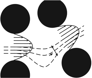
Diffusion across nearby streamlines leads to a local averaging over the transverse spatial structure of the velocity field. Thus, transverse diffusion in real space translates to an averaging effect in velocity space. We quantify the impact of the spatial structure on this averaging process through an effective shear rate, characterized in terms of flow properties. Transport along the longitudinal direction is then described in terms of equidistant spatial steps along particle trajectories, together with transit times according to the velocity process. Due to the nature of the velocity transitions induced by diffusion, which, as we will show, correspond to a dispersive process in velocity space, we name the approach the diffusing-velocity random walk (DVRW). A conceptual illustration of the DVRW approach for advective–diffusive transitions is presented in figure 1.

Figure 1. Conceptual illustration of the central concepts behind the diffusing-velocity random walk. As Lagrangian particles are transported, they undergo advective changes in velocity due to variability along streamlines as well as diffusion-induced averaging over, and transitions to, nearby streamlines. The transverse variability of the flow field is encoded in a velocity-dependent effective shear rate  $\alpha_e(v)$, which is determined by statistical properties of the flow field. This conceptual illustration is two dimensional and includes the presence of a solid phase (black circles), but the proposed approach is applicable also to three dimensions and arbitrary flow fields characterized by well-defined characteristic lengths along the longitudinal and transverse directions, as developed in detail in the main text.
The general outline of the paper is as follows. First, in § 2 we discuss the description of transport as a spatial-Markov process in general terms. Section 3 is devoted to the formulation of the DVRW approach, incorporating the impact of advective and diffusive velocity transitions. In § 4 we present some general considerations about Eulerian velocity statistics. These are then employed to relate the effective shear rate to flow characteristics in § 5. In § 6 we develop predictions for asymptotic longitudinal dispersion in the presence of both advective and diffusive transitions. Overall conclusions are presented in § 7, and some supporting technical derivations and numerical validation results may be found in the appendices.
2. Transport as a spatial-Markov process
We present, as a starting point, a generic formulation of transport as a spatial-Markov process (Le Borgne et al. Reference Le Borgne, Dentz and Carrera2008). We start from a discrete formulation and then proceed to consider its continuum limit. Finally, we provide general forms for the dynamical equations of some key transport quantities. This general formulation will be adapted to describe the role of advective and diffusive transitions in the sections that follow.
2.1. Discrete formulation
The velocity magnitudes  $V_k$ after
  $k$ spatial steps of fixed length
  ${\rm \Delta} s$ along streamlines are assumed to form a Markov chain. This spatial-Markov velocity process is characterized by its transition probabilities. Discretizing velocity magnitudes into classes, the transition probabilities
  $r_{ij}(s)$ describe the probability that a tracer particle will be in class
  $i$ at distance
  $s+{\rm \Delta} s$, given that it was in class
  $j$ at distance
  $s$.
$s$.
We consider transport to be advection dominated along the local flow direction, with diffusion playing a role locally along the transverse direction(s). At a given velocity  $v$, a spatial step is associated with a duration
  ${\rm \Delta} s/v$. The time
  $T_k$ after
  $k$ spatial steps is thus described by the stochastic recursion relation
 \begin{equation} T_{k+1}=T_k+\frac{{\rm \Delta} s}{V_k}, \end{equation}
with the initial time  $T_0=0$. The distribution of initial velocities
  $V_0$ is determined by the initial spatial distribution of scalar, which is mapped onto the initial distribution of velocities according to the Eulerian velocity field. For example, an homogeneous spatial distribution corresponds to velocities distributed according to the Eulerian velocity probability density function (PDF), which will be discussed in detail in § 4. In what follows, we will characterize the Markov chain describing the evolution of velocity along a particle's trajectory through its transition probabilities, which depend on the statistical properties of the underlying flow field. The evolution of particle longitudinal positions (along the mean flow direction) is then modelled as
 \begin{equation} X_{k+1} = X_k+\frac{k{\rm \Delta} s}{\chi}, \end{equation}
where  $\chi$ is the average tortuosity, which can be computed as the spatial average of the magnitude of Eulerian velocities divided by the spatial average of their projection along the mean flow direction (Koponen, Kataja & Timonen Reference Koponen, Kataja and Timonen1996; Puyguiraud et al. Reference Puyguiraud, Gouze and Dentz2019b).
The use of the average tortuosity to relate longitudinal displacements to displacements along streamlines is common in spatial-Markov models, and it has been applied successfully to describe transport at the pore scale (Puyguiraud et al. Reference Puyguiraud, Gouze and Dentz2019a,b). We will assume this approximation in the following developments. For completeness and clarity, we first briefly discuss some of its limitations and possible extensions. An important limitation is the inability to account for recirculation zones, which, if present, can be reached by diffusion and lead to long retention times before solute can again exit by diffusion. Such effects would be mostly naturally included in the present framework by introducing transition probabilities into an additional zero-velocity state, with distributed retention times with statistics determined by diffusion and the geometry of recirculation zones, in the spirit of mobile-immobile or multi-rate mass transfer models (see, e.g. Coats & Smith Reference Coats and Smith1964; Haggerty & Gorelick Reference Haggerty and Gorelick1995; Comolli et al. Reference Comolli, Hidalgo, Moussey and Dentz2016). Such an approach could in addition be used to account for retention times due to sorption and desorption and related effects. Similarly, the average-tortuosity approximation does not explicitly account for local flow reversal, and it is in general not expected to be adequate if a strong variability in tortousity, rather than in velocity, is responsible for the main effects of transport variability across streamlines. At the expense of greater model complexity and difficulty of parameterization, the present approach could in principle be used in conjunction with variable tortuosity, in terms of statistics or mean values conditioned on longitudinal position and/or velocity. Flow reversal, if important, would require allowing for negative displacements in longitudinal position to be associated with steps along streamlines.
An important simplification brought about by the average-tortuosity approximation relates to the description of quantities at fixed longitudinal distance from injection. An important example, which we will discuss below, are breakthrough curves, representing mass flux per unit time at fixed control planes transverse to the mean flow direction. Under this approximation, distributions on a control plane at distance  $x$ from injection coincide with distributions at fixed distance
  $s=\chi x$ measured along streamlines. Therefore, fixed-
 $s$ statistics, which are most naturally obtained in a spatial-Markov model, directly determine control-plane statistics. In general, the relationship between fixed-
 $s$ and fixed-
 $x$ distributions is more complex and depends also on the statistics of tortuosity.
2.2. Continuum limit
As we will see, it is convenient in our formulation to define velocity classes related to diffusive averaging in terms of the discretization  ${\rm \Delta} s$. Using this approach, the continuum limit of
  ${\rm \Delta} s\to 0$ will also correspond to infinitesimal velocity class sizes and transition times
  ${\rm \Delta} s/V_k$. Therefore, it will be associated with a continuous stochastic process for the random time needed to travel distance
  $s$ along times. In this sense, the recursion relation (2.1) in the limit
  ${\rm \Delta} s\to 0$ defines a stochastic process
 \begin{equation} T(s)=\int_0^s \frac{\textrm{d} s'}{V_S(s')}, \end{equation}
where  $V_S$ is the Markov process corresponding to the continuum limit of the Markov chain defined by the transition probabilities introduced above.
The change in a quantity  $q_i(s)$, depending on velocity class
  $i$ and given distance
  $s$, due to all possible velocity transitions over a step
  ${\rm \Delta} s$ is given by
  $q_i(s+{\rm \Delta} s)-q_i(s)=\sum_{j\neq i}r_{ij}q_j$, where
  $r_{ij}$ is the transition probability from class
  $j$ to class
  $i$ and the sum extends over all velocity classes
  $j\neq i$. Let
  $q(v;s)$ be the associated continuous density, i.e.
  $q_i(s)=\int_{b_i}^{b_{i+1}} \textrm {d}v\,q(v;s)\approx {\rm \Delta} v_i q(v_i;s)$, where the velocity class
  $i$ is defined as comprising velocities
  $v\in [b_i,b_{i+1}[$ and
  ${\rm \Delta} v_i = b_{i+1}-b_i$. Then, in the limit
  ${\rm \Delta} s\to 0$,
 \begin{equation} \frac{\partial q(v;s)}{\partial s} = \mathcal{L} q(v;s), \end{equation}
where  $\mathcal {L}$ is the continuum operator describing velocity transitions, defined through
 \begin{equation} \mathcal{L} q(v_i;s) = \lim_{{\rm \Delta} s\to0}\frac{r_{ij}(s)-\delta_{ij}}{{\rm \Delta} s{\rm \Delta} v_i}. \end{equation}
We are now in a position to develop general forms for the dynamical equations governing transport quantities. The actual dynamics will then depend on the particular form of transition operator  $\mathcal {L}$, which embodies the transition probabilities of the spatial-Markov velocity process.
The space-Lagrangian velocity PDF describes the velocity point statistics of Lagrangian particles at a fixed distance travelled along streamlines. Note that, in the presence of diffusion, the same particle trajectory spans multiple streamlines. In addition to advective transport along streamlines, diffusion transverse to the local flow direction induces transitions to nearby streamlines, as will be formalized in what follows. As discussed above, under the average-tortuosity approximation adopted here, this presents no further difficulties, as transport in the average flow direction can be directly related to the total distance travelled along (a collection of) streamlines. Using (2.4), we obtain a master equation for its evolution in space,
 \begin{equation} \frac{\partial p_S(v;s)}{\partial s}=\mathcal{L} p_S(v;s), \end{equation}
with no-flux boundary conditions for velocity in order to conserve probability. For a given initial condition in  $s$, corresponding to the velocity distribution at
  $s=0$, the solution of (2.6) represents the distribution of velocities at fixed
  $s$ over an ensemble of trajectories, irrespective of the arrival time. Equation (2.6), together with the initial condition, defines the continuous stochastic velocity process
  $V_S$.
Other important transport quantities are breakthrough curves (mass flux per unit time at a given distance) and concentration profiles (PDF of positions at a given time). Due to correlations introduced by the velocity process, it is convenient to first consider the joint probability density of velocity and arrival time at a fixed distance, defined such that  $\psi (v,t;s)\,\textrm {d} v\,\textrm {d} t$ is the probability of arriving at a given distance
  $s$ at a time in
  $[t,t+\textrm {d} t[$ and with velocity in
  $[v,v+\textrm {d} v[$. Proceeding similarly to above, see appendix A for details, we obtain the dynamical equation
 \begin{equation} \frac{\partial\psi(v,t;s)}{\partial s}+v^{-1}\frac{\partial\psi(v,t;s)}{\partial t}=\mathcal{L}\psi(v,t;s). \end{equation}
The boundary and initial conditions are no-flux in velocity as before, along with  $\psi (v,t;0)=p_S(v;0)\delta (t)$ and
  $\psi (v,0;s)=0$. Note that, by definition, we have
  $\int_0^\infty \textrm {d} t\,\psi (v,t;s)=p_S(v;s)$. Indeed, integrating out
  $t$ in (2.7) leads to (2.6) for the space-Lagrangian velocity PDF. The first passage time PDF at distance
  $s$ is given by
  $\phi (t;s)=\int_0^\infty \textrm {d} v\,\psi (v,t;s)$. Particle positions as a function of time are given by
  $X_T(t)=X[S(t)]=S(t)/\chi$, where
  $S(t)$ describes the random distance travelled by advection along streamlines. Since
  $S(t)$ always increases with time, and longitudinal position is approximated using the average tortuosity, each Lagrangian particle in this model crosses a given longitudinal position at most once. The breakthrough curves, normalized to unit total mass, are thus related to the first passage times by
  $f(t;x)=\phi (t;\chi x)$.
In order to obtain the PDF of particle positions at a given time, we employ the concept of subordination (Feller Reference Feller2008; Meerschaert & Sikorskii Reference Meerschaert and Sikorskii2012), which may be thought of as a stochastic change of independent variable. For example, consider  $X_U(u)$ describing the random position of a particle as a function of time
  $u$ spent moving. If the time spent moving as a function of total time
  $t$ is itself a random variable
  $U(t)$, the position of the particle as a function of total time is given by the subordinated process
  $X_T(t)=X_U[U(t)]$. The total time
  $T(u)$ given time
  $u$ spent moving is called the subordinator, and
  $U(t)$ is called its conjugate process. Here, the time
  $T(s)$ as a function of fixed distance
  $s$ plays the role of the subordinator, and
  $S(t)$ is its conjugate process at fixed time
  $t$. According to the theory of subordination, the PDF of
  $S(t)$ is then given by Feller (Reference Feller2008), Benson & Meerschaert (Reference Benson and Meerschaert2009) and Meerschaert & Sikorskii (Reference Meerschaert and Sikorskii2012):
 \begin{equation} h(s;t)=\int_0^t \textrm{d} t'\,\frac{\partial f(t';s)}{\partial s}. \end{equation}
Integrating out velocity in (2.7), and noting that, as reflected by the boundary conditions, conservation of probability leads to the integral on the right-hand side vanishing, this may be written as
 \begin{equation} h(s;t)=\int_0^\infty \textrm{d} v\, v^{-1}\psi(v,t;s). \end{equation}
By definition,  $h(s;t)\,\textrm {d} s$ is the probability of having travelled a distance in
  $[s,s+\textrm {d} s[$ along streamlines by time
  $t$. The spatial concentration, normalized to unit mass, is the PDF of particle positions
  $X_T(t)=S(t)/\chi$, and it is therefore given by
  $c(x;t)=\chi h(\chi x;t)$.
Finally, consider the time-Lagrangian velocity PDF, describing particle velocities at fixed time rather than distance, that is, the PDF of velocities  $V_T(t)=V_S[S(t)]$ at fixed
  $t$. Using the same approach as before leads to
 \begin{equation} p_T(v;t)=\int_0^\infty \textrm{d} s\,v^{-1}\psi(v,t;s). \end{equation}
We note that equations for multi-point PDFs, corresponding to the joint PDFs of quantities at more than one time or distance, may be obtained through similar procedures, see Dentz et al. (Reference Dentz, Kang, Comolli, Le Borgne and Lester2016).
3. The diffusing-velocity random walk
As outlined in the introduction, velocity transitions may occur due to both transverse diffusion and velocity variability along each streamline. We now proceed to quantify the impact of these two processes within the generic spatial-Markov framework outlined in the previous section. To this end, we first present an adapted derivation of the formulation of advective velocity transitions developed by Dentz et al. (Reference Dentz, Kang, Comolli, Le Borgne and Lester2016). We then develop a new approach to quantify the impact of transverse diffusion on velocity transitions. Finally, we combine the two to arrive at the general DVRW framework.
3.1. Advective transitions
We consider first advective transitions along streamlines, in the absence of diffusion. Let  $r^{\,A}_{ij}$ be the velocity transition probabilities of the spatial-Markov process associated with advective transitions, i.e. due to changes in velocity along a streamline. In order to characterize the continuum limit
  ${\rm \Delta} s\to 0$, we make use of the fact that the velocity process is Markov, with some correlation length
  $\ell_{//}$ corresponding to the longitudinal correlation length of the velocity field. We write, to first order in
  ${\rm \Delta} s$,
 \begin{equation} r^{\,A}_{ij}=\frac{{\rm \Delta} s}{\ell_{//}}\beta_{ij}(1-\delta_{ij})+ \left[1-\frac{{\rm \Delta} s}{\ell_{//}}(1-\beta_{ii})\right]\delta_{ij}, \end{equation}
where  $\delta_{\cdot \cdot }$ is the Kronecker delta. The first term corresponds to the probability of changing velocity class and the second of staying in the same class. The
  $\beta_{ij}$ encode the dependency of the transition probabilities on the velocity classes. To ensure normalization, i.e.
  $\sum_i r^{\,A}_{ij}=1$, we must have
  $\beta_{jj}=1-\sum_{i\neq j}\beta_{ij}$.
Recall that  $r_{ij}-\delta_{ij}$, seen as a function of velocity class
  $j$ for each velocity class
  $i$, defines an operator describing the change in velocity class due to a transition, see (2.5). Equation (3.1) leads, to first order in
  ${\rm \Delta} s$, to
 \begin{equation} r^{\,A}_{ij}-\delta_{ij} = \frac{{\rm \Delta} s}{\ell_{//}}(\beta_{ij}-\delta_{ij}). \end{equation}
Thus, in the continuum limit, we recover the dynamical equations of § 2 with a transition operator  $\mathcal {L}=\mathcal {L}_A$ describing advective transitions along streamlines. This is in general an integral (as opposed to differential) operator, because the velocity transitions may be long range in velocity space. Indeed, according to (2.5), we have, for an arbitrary density
  $q(v)$ as a function of velocity
  $v$,
$v$,
 \begin{equation} \mathcal{L}_A q(v) = \ell_{//}^{-1}\int_0^\infty \textrm{d} v'\left[\beta(v\,|\,v')-\delta(v-v')\right]q(v'), \end{equation}
where  $\beta$ is the transition PDF along streamlines (units
  $[\beta ]=1/V=T/L$), i.e.
  $\beta (v\,|\,v')\,\textrm {d} v$ is the transition probability from velocity
  $v'$ to a velocity in
  $[v,v+\textrm {d} v[$. It corresponds to the limit
 \begin{equation} \beta(v_i\,|\,v_j)=\lim_{{\rm \Delta} s \to 0}\frac{\beta_{ij}}{{\rm \Delta} v_i}. \end{equation}
In this case, it has been shown that, under ergodicity and incompressibility, the equilibrium space-Lagrangian velocity PDF is the flux-weighted Eulerian PDF (see § 4), irrespective of the initial condition, and the equilibrium time-Lagrangian velocity PDF is the Eulerian velocity PDF (Dentz et al. Reference Dentz, Kang, Comolli, Le Borgne and Lester2016; Puyguiraud et al. Reference Puyguiraud, Gouze and Dentz2019a,b). Non-stationary transition probabilities can be encoded in  $s$-dependent
  $\beta_{ij}$ and would lead to
  $s$-dependent
  $\beta (v\,|\,v')$. We note that, in natural media such as geological structures, non-stationarity is typically most naturally described in terms of distance
  $x$ along the mean flow direction, which under the average-tortuosity approximation is directly related to
  $s$ via
  $s=\chi x$.
The details of the dynamics depend on the choice of process governing the transition probabilities between velocity classes and on the underlying Eulerian velocity distribution. As in Dentz et al. (Reference Dentz, Kang, Comolli, Le Borgne and Lester2016), we will focus on the case of Bernoulli relaxation. This process is defined by the transition probabilities
 \begin{equation} r^{\,A}_{ij} = \textrm{e}^{-{\rm \Delta} s/\ell_{//}}\delta_{ij}+\left(1-\textrm{e}^{-{\rm \Delta} s/\ell_{//}}\right)p^{\infty}_i. \end{equation}
The physical interpretation of this set-up is as follows. Velocities persist on the scale of the correlation length  $\ell_{//}$, and when a transition occurs, the probability of the new velocity being in class
  $i$ is given by the prescribed equilibrium probability
  $p^{\infty }_i$. Thus, the velocity distribution ‘relaxes’ towards the equilibrium distribution on a spatial scale of the order of
  $\ell_{//}$. The exponential probability of persistence in (3.5) is a consequence of the assumption that the probability of transition per unit length is constant and equal to
  $1/\ell_{//}$. In this sense, the Bernoulli process may be seen as the simplest Markov process converging to a given equilibrium distribution on a given scale. For small
  ${\rm \Delta} s$, this corresponds, according to (3.1), to
  $\beta_{ij}=p^{\infty }_i$, the equilibrium probability of velocity class
  $i$. The continuum-limit transition PDF is given by
  $\beta (v_i\,|\,v_j)=p^\infty (v_i)$, the equilibrium PDF evaluated at
  $v_i$, irrespective of
  $v_j$. As mentioned above, the equilibrium PDF should in this context be taken equal to the flux-weighted Eulerian PDF.
Under the Bernoulli relaxation process, all velocities relax towards the equilibrium distribution at the same spatial rate. Other processes may be used to account for velocity-dependent relaxation while retaining the Markov property and stationarity of the transitions. For example, a process based on the classical Ornstein–Uhlenbeck process describing temporal velocity fluctuations in Brownian motion (Uhlenbeck & Ornstein Reference Uhlenbeck and Ornstein1930) has been successfully employed to capture slower spatial relaxation of low velocities in connection with transport in a heterogeneous porous medium (Puyguiraud et al. Reference Puyguiraud, Gouze and Dentz2019a). Conversely, in the presence of preferential high-velocity channels, one expects stronger correlation, and consequently slower spatial relaxation, at high velocities. In general, in the present formulation, velocity-dependent relaxation corresponds to  $j$-dependent
  $\beta_{ij}$. From (3.2), where the latter always occur in the combination
  $\beta_{ij}/\ell_{//}$, we see that this leads, in effect, to a velocity-dependent correlation length. In this sense, we may interpret
  $\ell_{//}/\sum_{i\neq j}\beta_{ij}=\ell_{//}/(1-\beta_{jj})$ as an effective correlation length associated with velocity class
  $j$. The probability of leaving a velocity class in a given step is then inversely proportional to the effective correlation length. Note that the
  $\beta_{ij}$ are in principle arbitrary, so long as probability is conserved,
  $\sum_i \beta_{ij}=1$, and they lead to the correct equilibrium distribution, the flux-weighted Eulerian PDF. Even when the overall velocity distribution across all particles has reached equilibrium, single-particle velocities remain dynamic, with the spatial velocity series of each particle undergoing purely advective transport being directly determined by the choice of
  $\beta_{ij}$.
3.2. Diffusive transitions
Next, we examine the role of diffusion, disregarding advective transitions for the moment. This corresponds to the limit of infinite correlation length  $\ell_{//}\to \infty$. It is directly applicable to stratified flow, where velocity is constant along each streamline, and velocity transitions are due only to transverse diffusion across streamlines. This will lead us to discrete and continuous formulations of transverse diffusion as a spatial-Markov process.
3.2.1. Discrete formulation
The characteristic transverse length explored by diffusing particles in a time interval  ${\rm \Delta} t$ is given by
  $\sqrt {2D{\rm \Delta} t}$, and a spatial displacement of length
  ${\rm \Delta} s$ at velocity
  $v$ corresponds to a duration
  ${\rm \Delta} t = {\rm \Delta} s/v$. The local averaging of velocities due to transverse diffusion during this time interval depends on the spatial structure of the velocity field. The cornerstone of our approach is the notion of a velocity-dependent effective shear, see figure 1. We describe the local variation of the flow around regions of velocity
  $v$ in terms of an effective transverse shear rate magnitude
  $\alpha_{e}(v)$, so that the range of velocities averaged by diffusion around velocity
  $v$ is given by
 \begin{equation} {\rm \Delta} v(v)=\alpha_{e}(v)\sqrt{2D{\rm \Delta} s/v}. \end{equation}
The actual transverse velocity gradient magnitude depends in general on position, and a given value of velocity at a randomly chosen spatial location is thus associated with a PDF of possible shear values. Our approach may be seen as a mean-field formulation associating an average shear rate  $\alpha_{e}(v)$ with each velocity value
  $v$.
$v$.
We consider for now that the effective shear rate  $\alpha_{e}(v)$ is known as a function of velocity magnitude, and we will derive the consequences for transport. Section 5 will be devoted to relating the effective shear rate to physical properties, in particular the underlying flow statistics. Note that, analogously to above with the transition PDF
  $\beta$ characterizing advective transitions, we have assumed that
  $\alpha_e(v)$ does not depend on distance
  $s$. A non-stationary model can be formulated using the present approach, but we refrain from exploring it here for simplicity.
The changes in velocity at each step are modelled as a spatial-Markov process, which is characterized by the diffusive transition probabilities  $r^{\,D}_{ij}$ from each velocity class
  $j$ to each velocity class
  $i$ over a step
  ${\rm \Delta} s$ along the flow direction. We discretize velocity magnitudes
  $v$ into classes
  $v\in [b_i,b_{i+1}[$. The width
  ${\rm \Delta} v_i=b_{i+1}-b_i$ of each class is determined by transverse diffusive averaging according to (3.6). That is, we set
  ${\rm \Delta} v_i = \alpha_i\sqrt {2D{\rm \Delta} s/v_i}$, where
  $v_i$ is the average velocity within class
  $i$ and
  $\alpha_i=\alpha_{e}(v_i)$. A recursive construction valid in the limit of small class widths is given in appendix B. The class widths
  ${\rm \Delta} v_i$ vanish in the limit
  ${\rm \Delta} s \to 0$, so that small-
 ${\rm \Delta} v_i$ approximations are reasonable for small
  ${\rm \Delta} s$. The same is true of the transition times
  ${\rm \Delta} s/v_i$.
In each step  ${\rm \Delta} s$, diffusion averages over the current velocity class, and induces transitions to the nearest classes according to the transition probabilities
 \begin{equation} r^{\,D}_{ij}=r_j^+\delta_{i,j+1}+r_j^-\delta_{i,j-1}, \end{equation}
where  $r_j^\pm$ are the transition probabilities from class
  $j$ to class
  $j\pm 1$, with
  $r_j^++r_j^-=1$. For the
  $j=0$ velocity class, we have
  $r^+_0=1$ and
  $r^-_0=0$, since there is no class below. Conversely, for the highest velocity class, transitions are always to the class below. For the remaining classes, the diffusive transition probabilities are obtained as follows. By construction, during a transition, diffusion homogenizes a transverse length corresponding to a velocity class. The transition is thus associated with a transition time
  ${\rm \Delta} t={\rm \Delta} s/v_j$, where
  $v_j$ is the (arithmetic) average velocity in the class. However, for a given
  ${\rm \Delta} t$, the amount of distance travelled at a given velocity
  $v$ is proportional to
  $v$. This means that the probability of a particle having velocity
  $v$ when it finishes the spatial step
  ${\rm \Delta} s$ is proportional to
  $v$. In other words, the velocity distribution within a class after a spatial transition is flux weighted. Imposing a diffusive transition to the velocity class below if the particle has a velocity lower than the class average (and to the class above otherwise) leads to
  $r^-_j=\int_{b_j}^{v_j}\textrm {d} v\, v / \int_{b_j}^{b_{j+1}}\textrm {d} v'\, v'$. Thus,
  $r^-_j=(v_j^2-b_j^2)/(b_{j+1}^2-b_j^2)$. Approximating the class average
  $v_j$ by the class centre, we have
  $b_j=v_j-{\rm \Delta} v_j/2$ and
  $b_{j+1}^2-b_j^2=(b_{j+1}-b_j)(b_{j+1}+b_j)=2v_j{\rm \Delta} v_j$, so that
 \begin{equation} r^\pm_j = \frac{1}{2}\pm\frac{{\rm \Delta} v_j}{8v_j}. \end{equation}
3.2.2. Continuum limit
According to the previous construction, as  ${\rm \Delta} s\to 0$, both the velocity class widths
  ${\rm \Delta} v_i\to 0$ and the corresponding transition times
  ${\rm \Delta} s/v_i\to 0$, indicating that this corresponds to a genuine continuous limit. We now examine this limit in detail, and we obtain the continuum stochastic process underlying diffusive transitions, as well as the associated transition operator.
In the continuum limit, (3.7) leads to the operator  $\mathcal {L} = \mathcal {L}_D$ associated with diffusive transitions, see (2.5). Because diffusive transitions are local, the corresponding operator is differential. For an arbitrary density
  $q$,
$q$,
 \begin{equation} \mathcal{L}_D q(v)=\frac{\partial}{\partial v} \left[\gamma(v)\frac{\partial q(v)}{\partial v}-\mu(v)q(v)\right]; \end{equation}
see appendix C for details on the derivation. The spatial velocity diffusivity  $\gamma$ (
 $[\gamma ]=V^2/L=L/T^2$) corresponds to the limit
  $\gamma (v_i)=\lim_{{\rm \Delta} s\to 0}{\rm \Delta} v_i^2 /(2{\rm \Delta} s)$ and is given by
 \begin{equation} \gamma(v)=Dv^{-1}\alpha_{e}(v)^2, \end{equation}
and
 \begin{equation} \mu(v)=\left(v^{-1}-\frac{\partial}{\partial v}\right)\frac{\gamma(v)}{2} \end{equation}
is a spatial velocity drift ( $[\mu ]=V/L=1/T$). The first term in this drift is due to the fact that particles are more likely to transition to higher velocities by diffusion within a class, due to the flux-weighting effect discussed above. The second arises because velocity classes, corresponding to spatial averaging by diffusion over a constant spatial step, have velocity-dependent sizes. Thus, particles spend longer distances at velocities where classes are smaller, giving rise to an effective drift towards these velocities. The size of the velocity class decreases with velocity, because shorter crossing times are associated with smaller diffusion lengths, and increases with effective shear, because higher effective shear corresponds to stronger variation of velocity over the same transverse distance (see figure 1). In particular, the space-Lagrangian velocity PDF obeys the master equation (2.6) with
  $\mathcal {L}=\mathcal {L}_D$. The boundary conditions in
  $v$ must ensure conservation of probability, so that we have the no-flux condition
  $\gamma \partial p_S/\partial v-\mu p_S=0$ at the minimum and maximum velocities.
3.3. Combining advective and diffusive transitions
We now combine the diffusive and advective transition mechanisms to obtain the complete transition probabilities of the DVRW framework, see figure 1. We impose that, if (and only if) a particle does not undergo an advective transition along a streamline, diffusion causes a transition to one of the nearest velocity classes. That is, the transition probabilities in the presence of both advection and diffusion become
 \begin{equation} r_{ij}=r^{\,A}_{ij}(1-\delta_{ij})+r^{\,A}_{jj}\left(r_j^+\delta_{i,j+1}+r_j^-\delta_{i,j-1}\right). \end{equation}
Thus, to first order in  ${\rm \Delta} s$, the changes in velocity class are determined by
 \begin{equation} r_{ij}-\delta_{ij} = \frac{{\rm \Delta} s}{\ell_{//}}(\beta_{ij}-\delta_{ij})+r_j^+ \delta_{i,j+1}-\delta_{ij}+r_j^-\delta_{i,j-1}. \end{equation}
 Due to the Markovian nature of the process, the somewhat artificial requirement that diffusive transitions occur only when an advective transition does not occur is inconsequential in the limit of small  ${\rm \Delta} s$. This can be seen from the fact that
  $r_{ij}-\delta_{ij}$, which defines the operator characterizing the change in velocity classes over
  ${\rm \Delta} s$, is composed of the sum of terms associated with purely advective and purely diffusive velocity transitions to leading order in
  ${\rm \Delta} s$; thus, the transition operator in the continuum limit becomes the sum of the diffusive and advective contributions. This leads to the same continuum-limit dynamical equations as before, with the transition operator now given by
  $\mathcal {L} = \mathcal {L}_A + \mathcal {L}_D$, see (3.3) and (3.9), representing the effect of both advective and diffusive transitions. That is, for an arbitrary density
  $q$,
$q$,
 \begin{align} \mathcal{L}q(v) = \ell_{//}^{-1}\int_0^\infty \textrm{d} v'\left[\beta(v\,|\,v')-\delta(v-v')\right]q(v') +\frac{\partial}{\partial v}\left[\gamma(v)\frac{\partial q(v)}{\partial v}-\mu(v)q(v)\right]. \end{align}
Note that, if there is no velocity variation along streamlines, or equivalently  $\ell_{//}\to \infty$, then
  $r^{\,A}_{ij}=\delta_{ij}$, and we recover the pure diffusion formulation, valid for stratified flow. Conversely,
  $D=0$ recovers the purely advective scenario discussed above.
4. Eulerian velocity statistics
As seen from (3.9)–(3.11), the effective shear  $\alpha_{e}(v)$ plays a key role in quantifying diffusive transitions. In order to relate it to flow properties, and in particular to velocity statistics, let us first discuss some properties of the Eulerian PDF of velocity magnitudes, defined as the probability of finding a certain velocity magnitude value at a uniformly random spatial location.
Denoting the spatial velocity field magnitude at position  $\boldsymbol x$ in a domain
  $\varOmega$ by
  $v_E(\boldsymbol x)$, the Eulerian velocity PDF is then defined as
 \begin{equation} p_E(v) = |\varOmega|^{-1}\int_\varOmega \textrm{d}\boldsymbol x\, \delta[v-v_E(\boldsymbol x)], \end{equation}
where  $\delta (\cdot )$ is the Dirac delta, and for a
  $d$-dimensional spatial domain
  $A$,
$A$,  $|A|$ denotes its measure (number of elements, area or volume, respectively, for
  $d=1,2,3$). Assuming a smooth, non-constant velocity field, changing variables in the Dirac delta (Hörmander Reference Hörmander2015) leads to
 \begin{equation} p_E(v) = \int_{\varLambda(v)}\frac{\textrm{d}\sigma(\boldsymbol x)}{|\varOmega||\nabla v_E(\boldsymbol x)|}. \end{equation}
In  $d$ spatial dimensions,
  $\varLambda (v)$ is the
  $(d-1)$-dimensional spatial surface where the velocity field has magnitude
  $v$,
$v$,  $\varLambda (v)=\{\boldsymbol x \in \varOmega : v_E(\boldsymbol x) = v\}$, and
  $d\sigma (\boldsymbol x)$ is the corresponding
  $(d-1)$-area element at the point
  $\boldsymbol x$ on
  $\varLambda (v)$. The harmonic average of the local shear rate magnitude
  $|\nabla v_E(\boldsymbol x)|$ over this surface is given by
 \begin{equation} \alpha_h(v) = \left[|\varLambda(v)|^{-1}\int_{\varLambda(v)} \frac{\textrm{d}\sigma(\boldsymbol x)}{|\nabla v_E(\boldsymbol x)|}\right]^{-1}, \end{equation}
leading to
 \begin{equation} p_E(v) = \frac{|\varLambda(v)|}{|\varOmega|\alpha_h(v)}, \end{equation}
which shows that the Eulerian PDF is directly related to the harmonic average of the local shear rate given a velocity magnitude. Note that this result is valid for an arbitrary smooth velocity field that is not constant. For a piecewise-smooth velocity field, the result applies piecewise. If the velocity field has fully degenerate maxima or minima, that is, regions of finite volume (in two dimensions, area) where velocity is constant, they yield Dirac-delta contributions corresponding to that velocity, with a probability mass (coefficient) given by the ratio of the region volume and  $|\varOmega |$. This can easily be seen from the definition of the Eulerian PDF, (4.1).
Throughout, an overline will denote the ensemble average (over tracer particles), and  $V_E$ will stand for a random variable distributed according to
  $p_E$, corresponding to the velocity at a uniformly random spatial point. Using the previous result, it follows that
 \begin{equation} \overline{\alpha_h(V_E)} = |\varOmega|^{-1}\int_0^\infty \textrm{d} v\, |\varLambda(v)|. \end{equation}
We introduce also the flux-weighted Eulerian PDF, defined according to
 \begin{equation} p_F(v)=\frac{v}{\overline{V_E}}p_E(v), \end{equation}
which plays an important role in our formulation.
We now consider the Eulerian PDF of velocities at a fixed distance  $s$ along streamlines. Let
  $\varOmega_\perp (s)$ be the
  $(d-1)$-dimensional cross-section of
  $\varOmega$ at fixed
  $s$, and let
  $\varLambda (v;s)=\{\boldsymbol x \in \varOmega_\perp (s) : v_E(\boldsymbol x) = v\}$ be the
  $(d-2)$-surface of constant velocity on
  $\varOmega_\perp (s)$. The gradient of the velocity magnitude transverse to the flow direction is given by
  $\nabla_\perp v_E$, where
  $\nabla_\perp = \nabla -(\boldsymbol v/|v|^2)\boldsymbol v\cdot \nabla$. Adapting the previous derivation,
 \begin{equation} p_E(v;s)=\frac{|\varLambda(v;s)|}{|\varOmega_\perp(s)|\alpha_h(v;s)}, \end{equation}
where  $\alpha_h(v;s)$ is the harmonic average of
  $|\nabla_\perp v_E|$ over
  $\varLambda (v;s)$. Note that the Eulerian velocity PDF at fixed
  $s$ is not sensitive to gradients along the flow direction; their contribution to the full PDF arises through their effect on the variation of
  $|\varLambda (v;s)|/\alpha_h(v;s)$ with
  $s$. For stratified flows, where velocity is constant along each streamline,
  $p_E(v;s)=p_E(v)$ always holds. This equality also holds for more general flows, as long as the point statistics of velocity over any given transverse plane coincide with those of the full domain. We will assume this to be the case in what follows for simplicity.
As an example, consider Poiseuille flow in  $d=2$ dimensions. The Eulerian velocity field is in this case given by
 \begin{equation} v_E(y) = v_M\left[1-\left(\frac{2y}{L}\right)^2\right], \end{equation}
where  $L=|\varOmega_\perp |$ is the transverse domain width,
  $y\in [-L/2,L/2]$ is the position in the transverse direction and
  $v_M$ is the maximum velocity, occurring at
  $y=0$. The full Eulerian PDF is equal to the PDF over the transverse direction, since there is no variability along the longitudinal direction. The absolute value of the gradient of velocity is uniquely determined by the velocity, and we have
 \begin{equation} \alpha_h(v)=\frac{4v_M}{L}\sqrt{1-\frac{v}{v_M}}. \end{equation}
Since the same absolute value of the gradient occurs at exactly two points (except at the maximum, where it is zero), we have  $|\varLambda (v)|=2$. According to (4.4), the Eulerian PDF is thus given by
 \begin{equation} p_E(v)=\frac{1}{2v_M\sqrt{1-v/v_M}}, \end{equation}
and the average velocity is  $\overline {V_E}=2v_M/3$. Note the square-root divergence near the maximum, which is in agreement with the discussion in appendix D for
  $d=1$, the effective dimension of variability of this flow field.
5. Effective shear rate
This section is devoted to linking the effective shear  $\alpha_{e}(v)$ rate to flow characteristics, in particular point statistics as encoded in the Eulerian PDF. In what follows, we will achieve this by requiring that the DVRW formulation satisfy two criteria in the limit of longitudinal correlation length
  $\ell_{//}\to \infty$ (i.e. when only diffusive transitions are present): (i) reproducing the asymptotic space-Lagrangian velocity PDF as distance
  $s\to \infty$; and (ii) reproducing the asymptotic Taylor dispersion coefficient as time
  $t\to \infty$.
5.1. Equilibrium velocity PDF
As shown in § 3.2, the space-Lagrangian velocity PDF for purely diffusive velocity transitions obeys the master equation  $\partial p_S(v;s)/\partial s = \mathcal {L}_D p_S(v;s)$, with the diffusive transition operator
  $\mathcal {L}_D$ given by (3.9). Thus, the equilibrium PDF solves
  $\mathcal {L}_Dp^{\infty }_S(v)=0$. Integrating this equation using no-flux boundary conditions, and imposing normalization, we obtain
 \begin{equation} p^{\infty}_S(v)=\frac{v}{\alpha_{e}(v)}\left[\int_0^\infty \textrm{d} v'\,\frac{v'}{\alpha_{e}(v')}\right]^{-1}. \end{equation}
According to Taylor dispersion theory, the equilibrium distribution of velocities for a stratified flow after diffusion samples the full transverse variability is the flux-weighted Eulerian distribution,  $p^{\infty }_S(v)=p_F(v)$. When only velocity transitions by transverse diffusion are considered, which is equivalent to taking the limit of an infinite longitudinal correlation length
  $\ell_{//}$ in (3.14) for the transition operator
  $\mathcal {L}$, the DVRW becomes equivalent to transport in stratified flow. Asymptotic dispersion should then agree with the Taylor result.
According to (5.1),  $p^\infty_S(v) \propto v/\alpha_e(v)$, where the proportionality factor is
  $v$-independent and ensures normalization. Obtaining the flux-weighted Eulerian PDF, (4.6), as the space-Lagrangian equilibrium PDF thus requires
  $\alpha_{e}(v)\propto 1/p_E(v)$, so that
  $p^\infty_S(v)\propto v p_E(v)$. Therefore, we write for the effective shear rate
 \begin{equation} \alpha_{e}(v)=\frac{\overline{\alpha_{e}(V_E)}}{\delta vp_E(v)} \end{equation}
for  $v\in ]v_m,v_M[$ (and zero otherwise) and with
  $\delta v=v_M-v_m$ the difference between the maximum and minimum velocities. Note that we have fixed the velocity-independent coefficient in terms of the average effective shear rate
  $\overline {\alpha_{e}(V_E)}=\int_0^\infty \textrm {d} v\,p_E(v) \alpha_e(v)$. We will show shortly that this average is determined by asymptotic longitudinal dispersion. It is worth noting also that a physical instance of a velocity field in a finite domain always exhibits a finite maximum velocity. However, theoretical Eulerian PDFs, applying in principle to an infinite domain or an infinite number of domain realizations, may be defined for any positive velocity magnitude. We will later obtain a form of the effective shear rate which does not explicitly depend on the maximum and minimum velocity values and is suitable for direct computation for an arbitrary Eulerian PDF.
In order to provide intuition for the velocity dependence of the effective shear rate, consider the stratified flow profile shown in figure 2, corresponding to a cut in the direction transverse to a two-dimensional flow, which we name the  $M$-flow. This synthetic example, where the local shear magnitude is constant and equal to
  $\alpha$, is chosen to highlight the role of the multiplicity (number of spatial occurrences)
  $|\varLambda (v)|$ associated with each velocity. Velocity magnitude
  $v$ occurs
  $|\varLambda (v)|=\varLambda_M=4$ times for
  $v$ larger than a critical velocity
  $v_c$, and
  $|\varLambda (v)|=\varLambda_m=2$ times for
  $v<v_c$. This implies that the centre and outer parts of the flow cover velocity variations
  $\delta v_{M,m}=|v_{M,m}-v_c|$ over lengths
  $\ell_{M,m}=\varLambda_{M,m}\delta v_{M,m}/\alpha$, respectively. Similarly, the effective shear rate
  $\alpha_{e}^{M,m}\propto \delta v_{M,m}/\ell_{M,m}=\alpha /\varLambda_{M,m}$ for velocities above and below the critical velocity
  $v_c$. Noting that
  $p_E(v) \propto |\varLambda (v)|/\alpha$, see (4.4), we see that, indeed,
  $\alpha_{e}(v)\propto 1/p_E(v)$.

Figure 2. Transverse velocity magnitude profile for the  $M$-flow. The key relevant features of this illustrative example are: (i) the multiplicity (number of spatial occurrences) of velocity magnitudes above (below) the critical value
  $v_c$ is
  $\varLambda_M=4$ (
 $\varLambda_m=2$); (ii) the transverse gradient magnitude is constant. It is given by
  $\alpha =\delta v_m/(\ell_m/\varLambda_m)=\delta v_M/(\ell_M/\varLambda_M)$.
5.2. Longitudinal dispersion
Next, we turn to the asymptotic behaviour of longitudinal dispersion for purely diffusive velocity transitions, that is, in the limit of infinite longitudinal correlation length  $\ell_{//}$ as before. First, consider
  $V_T(t)$, the Lagrangian velocity process along particle trajectories as a function of travel time
  $t$. We have, for particle positions as a function of time,
 \begin{equation} X_T(t)=\chi^{-1}\int_0^t \textrm{d} t'\,V_T(t'), \end{equation}
from which  $\overline {X_T(t)} = \chi ^{-1}\int_0^t\textrm {d} t'\,\overline {V_T(t')}$.
The previous results imply that the equilibrium time-Lagrangian velocity PDF coincides with the Eulerian PDF, as expected from Taylor dispersion theory. To see this, consider the joint PDF of velocity and arrival time, (2.7) with  $\mathcal {L}=\mathcal {L}_D$. Integrating out
  $s$ and using (2.10) for the time-Lagrangian velocity PDF leads to
 \begin{equation} \frac{\partial p_T(v;t)}{\partial t}=p_S(v;0)\delta(t)+\mathcal{L}_D \int_0^\infty \textrm{d} s\, \psi(v,t;s). \end{equation}
For the steady state, we must thus have  $\int_0^\infty \textrm {d} s\, \psi (v,t;s)\propto p_F(v)$ and, therefore, using normalization,
 \begin{equation} p^{\infty}_T(v)=p_E(v). \end{equation}
Since, by definition, the time-Lagrangian PDF is the PDF of  $V_T(t)$, this implies that
  $\overline {V_T(t)}$ converges to
  $\overline {V_E}$ and, therefore, asymptotically,
  $\overline {X_T(t)}=\chi ^{-1}\overline {V_E}t$. Similarly, calculating
  $\overline {X^2_T(t)}$ leads to a longitudinal dispersion
 \begin{equation} \sigma^2(t) = \chi^{-2}\int_0^t \textrm{d} t' \int_0^t \textrm{d} t''\, \overline{V'_T(t')V'_T(t'')}, \end{equation}
where for late times  $V'_T(t)=V_T(t)-\overline {V_E}$ are the velocity fluctuations about the mean as a function of particle travel time. In a statistically stationary velocity field, the velocity correlations at late times depend only on the time difference,
  $\overline {V'_T(t')V'_T(t'')}=C_v(|t''-t'|)$. This yields the Green–Kubo relation (Kubo, Toda & Hashitsume Reference Kubo, Toda and Hashitsume1985) for the longitudinal dispersion coefficient,
 \begin{equation} D_{//}(t) = \frac{1}{2}\frac{\textrm{d}\sigma^2(t)}{\textrm{d} t}=\chi^{-2}\int_0^t \textrm{d} t'\, C_v(t'). \end{equation}
 The integral of the correlation function of velocity fluctuations, when it converges, is given by the product of the velocity autocorrelation and a correlation time. The first is proportional to  $\overline {V_E}^2$ and, for purely diffusive velocity transitions, the second is of the order of the diffusion time
  $\tau_D=L^2/(2D)$, where
  $L$ is the characteristic width of the domain cross-section. For large
  $t$, the integral can be approximated by extending the upper limit to infinity, leading to the asymptotic Taylor dispersion coefficient
 \begin{equation} D_T = \eta\frac{\overline{V_E}^2L^2}{\chi^2D}, \end{equation}
where  $\eta$ is a dimensionless coefficient characterizing the impact of the spatial organization of velocities. This is the form of the asymptotic longitudinal dispersion coefficient whenever the only mechanism for sampling velocity variability is diffusive (for example, in stratified flows), and it arises once the full variability has been sampled. While
  $\eta$ does not have a simple general form, it can be expressed in terms of the normalized velocity fluctuations within the transverse domain (see Aris (Reference Aris1956) and appendix E),
 \begin{equation} \nu(\boldsymbol y) = \frac{v_E(\boldsymbol y)}{\overline{V_E}}-1,\quad \boldsymbol y \in \varOmega_\perp. \end{equation}
In two dimensions, it is given by
 \begin{equation} \eta=L^{-3}\int_{-L/2}^{L/2} {\textrm{d}y} \left[\int_0^y {\textrm{d}y}'\, \nu(y')\right]^2, \end{equation}
whereas for an axisymmetric flow, we have, with  $\nu (r)$ in terms of the radial coordinate
  $r=\sqrt {\boldsymbol{y}\boldsymbol{\cdot} \boldsymbol{y}}$,
 \begin{equation} \eta=\frac{8}{L^4}\int_0^{L/2}\frac{\textrm{d} r}{r}\left[\int_0^r \textrm{d} r'\, r' \nu(r')\right]^2. \end{equation}
 The longitudinal dispersion coefficient corresponding to the DVRW for purely diffusive velocity transitions can be computed from the dynamical equation (2.7) for the joint PDF of velocity and arrival time, with the transition operator  $\mathcal {L}=L_D$ given by (3.9), together with (2.9) for the concentration PDF. As shown in appendix F.1, the asymptotic longitudinal dispersion coefficient is given by
 \begin{equation} D_\infty=\frac{I \delta v^2}{\overline{\alpha_{e}(V_E)}^2L^2}\frac{\overline{V_E}^2L^2}{\chi^2D}, \end{equation}
where the dimensionless coefficient  $I$ is a property of the Eulerian velocity PDF,
 \begin{equation} I = \int_0^\infty \textrm{d} v\, p_E(v)[C_E(v)-C_F(v)]^2. \end{equation}
Here, we have introduced  $C_{E,F}(v')=\int_0^v \textrm {d} v'\, p_{E,F}(v')$ as the Eulerian and flux-weighted Eulerian cumulative distribution functions, respectively.
We require that, when only diffusive transitions are present, the DVRW should reproduce the correct Taylor dispersion coefficient,  $D_\infty = D_T$. The first fraction in (5.12) must then equal
  $\eta$, see (5.8). This represents a second constraint on the average effective shear rate, which must be given by
 \begin{equation} \overline{\alpha_{e}(V_E)}=\sqrt\frac{I}{\eta}\frac{\delta v}{L}. \end{equation}
Together with (5.2), which enforced the first constraint of reproducing the correct asymptotic space-Lagrangian velocity PDF, we obtain
 \begin{equation} \alpha_{e}(v)=\frac{\sqrt{I/\eta}}{L p_E(v)}. \end{equation}
5.3. Role of statistical and spatial flow structure
From (4.5) and (5.14), we may write
 \begin{equation} \overline{\alpha_{e}(V_E)}=\sqrt\frac{I}{\eta\omega^2}\overline{\alpha_h(V_E)},\quad \omega=\frac{L}{\delta v}\int_0^\infty \textrm{d} v\, |\varLambda(v)|. \end{equation}
It may be surprising to observe that the ratio between the average effective shear and the average harmonic shear may differ from unity. The reason for this lies in the fact that the average harmonic shear rate, as defined by (4.3), does not provide information about the spatial organization of the velocity field. As we have seen, the velocity dependence of the effective shear rate is fixed by the Eulerian PDF. Different spatial organizations, however, lead to different Taylor dispersion coefficients, as encoded in  $\eta$, and this information must thus be included in the effective shear rate through its average value.
The impact on dispersion due solely to the point statistics of velocity is quantified by the coefficient  $I$. Using the definition of the Eulerian PDF, (4.1), we can express
  $I$ as a spatial integral,
 \begin{equation} I=|\varOmega_\perp|^{-3}\int_{\varOmega_\perp} \textrm{d}\boldsymbol y \left[\int_{\varOmega_\perp} \textrm{d}\boldsymbol y'\, \nu(\boldsymbol y')H[v_E(\boldsymbol y)-v_E(\boldsymbol y')]\right]^2, \end{equation}
where  $H(\cdot )$ is the Heaviside step function, meaning the inner integral extends over positions
  $\boldsymbol y'$ at which the velocity magnitude is smaller than at
  $\boldsymbol y$. Details on the derivation may be found in appendix F.1. The relationship between
  $I$ and
  $\eta$, i.e. between the impact of the statistical and spatial structures, becomes apparent when one considers certain special cases. Consider the following particular scenario in
  $d=2$ dimensions. First, assume constant
  $|\varLambda (v)|=\overline {|\varLambda (V_E)|}$. This case, for which we have also
  $\omega =\overline {|\varLambda (V_E)|}$, describes a situation where every velocity value appears
  $\omega$ times. Further assume that the velocity gradient magnitude is the same at each of these values, so that the shear rate magnitude may be written as a function of velocity. This implies the velocity profile has a simple spatial structure: the transverse domain is divided into subregions of equal length
  $L/\omega$, within each of which the velocity magnitude is monotonic. Furthermore, the velocity profile in adjacent regions is symmetric with respect to reflection across the boundary between them. Examples of this type (in
  $d=2$) are Couette flow, Poiseuille flow and triangular flow (corresponding to the
  $M$-flow, see figure 2, with
  $\delta v_M = 0$). This spatial structure, together with the fact that the integral of the velocity fluctuations in each subregion is null, leads, according to (5.17), to
 \begin{equation} I=L^{-3}\int_{-L/2}^{L/2} {\textrm{d}y}\left[\omega\int_0^y {\textrm{d}y}'\, \nu(y')\right]^2, \end{equation}
where the factor of  $\omega$ in the inner integral is due to the equal contribution of each subregion. Comparing to (5.10), this corresponds to
  $I=\omega ^2\eta$, so that, from (5.16a,b),
  $\overline {\alpha_{e}(V_E)}=\overline {\alpha_h(V_E)}$. However, breaking either of the previous hypotheses will in general result in
  $\overline {\alpha_{e}(V_E)}\neq \overline {\alpha_h(V_E)}$. For example, for an axisymmetric flow in
  $d=3$, we have
 \begin{equation} I=\frac{512}{L^6}\int_0^{L/2}\textrm{d} r\, r\left[\int_0^r \textrm{d} r'\, r' \nu(r')\right]^2, \end{equation}
so that, in general,  $\overline {\alpha_{e}(V_E)}\neq \overline {\alpha_h(V_E)}$ even in this simple scenario, compare (5.11). For illustration purposes, we computed
  $\eta$,
  $\omega$,
  $I$ and
  $\overline {\alpha_{e}(V_E)}/\overline {\alpha_h(V_E)}=\sqrt {I/(\eta \omega ^2)}$ for a number of simple stratified flows; the results are summarized in table 1.
Table 1. Values of  $\omega$,
  $I$ and
  $\eta$ for different stratified flows. The last column shows the value
  $\sqrt {I/(\eta \omega ^2)}$ of the ratio of the average effective shear to the harmonic average shear. Poiseuille flow for
  $d=3$ dimensions refers to a paraboloid profile in a cylindrical pipe. Coefficients for the
  $M$-flow are given in terms of
  $\lambda =\overline {|\varLambda (V_E)|}$; the polynomial coefficients for
  $\eta$ and
  $I$ are given by
  $c_i=(2368,-5760,5840,-2880,740,-96,5)$ and
  $d_i=(3904,-9600,10\,160,-4800,1100,-120,5)$,
  $i=0,\ldots ,6$, and
  $K(\lambda )=[(6-\lambda )^2-2(4-\lambda )^2]^2$.

With these results in mind, we identify
 \begin{equation} \ell_\perp = \sqrt\frac{\eta}{I}L \end{equation}
as the relevant length scale characterizing the variability of the velocity field in the transverse direction. When  $\sqrt {I/\eta }=\omega$, which holds in the simple scenario discussed above, this length scale coincides with the spatial period over which the Eulerian statistics of the velocity field repeat. Substituting in (5.15), the effective shear rate becomes
 \begin{equation} \alpha_{e}(v)=\frac{1}{\ell_\perp p_E(v)}. \end{equation}
This is the central result connecting the effective shear rate, which, together with the usual diffusion coefficient, determines the diffusive transitions of the DVRW, to flow properties. This connection was achieved by enforcing that the DVRW predictions for the asymptotic space-Lagrangian velocity distribution and longitudinal dispersion coefficient reduce to known results for purely diffusive velocity transitions, that is, for infinite velocity correlation length along streamlines.
The characteristic transverse length scale embodies the impact of the interplay between the statistical and spatial structures of the flow field in the transverse direction. In the absence of detailed information, it can be estimated based on the characteristic transverse length over which the full variability of the velocity structure is covered. If the spatial structure of the flow is known on a transverse section of the domain,  $I$ may be computed according to the corresponding Eulerian PDF, see (5.13), and
  $\eta$ may be obtained by computing the Taylor dispersion coefficient for a stratified flow characterized by the flow field magnitudes on the cross-section, see (5.8). The assumption of stationarity we have made here, according to which the effective shear rate does not depend on distance
  $s$, is satisfied when these quantities remain constant across different domain cross-sections. Although we do not explore the resulting non-stationary model here, the approach generalizes to cross-section-dependent quantities.
We numerically validated the formulation of diffusive transitions in terms of the effective shear rate for transport in some instances of the stratified flows from table 1 by comparing simulations of the discretized Lagrangian formulation of the DVRW to standard particle tracking simulations with a fixed time step. The results are discussed in appendix G.
6. Dispersion under heterogeneous advection and diffusion
In order to illustrate the impact of the interplay between advection and diffusion on transport, let us consider longitudinal dispersion under heterogeneous advection and diffusion. Following Dentz et al. (Reference Dentz, Kang, Comolli, Le Borgne and Lester2016), we consider as a rich example a gamma distribution of Eulerian velocities (figure 3 inset). The gamma PDF, expressed in terms of the mean velocity  $\overline {V_E}$, is given by
 \begin{equation} p_E(v)=\left(\frac{\theta v}{\overline{V_E}}\right)^\theta \frac{\textrm{e}^{-\theta v/\overline{V_E}}}{v\varGamma(\theta)}, \end{equation}
where  $\varGamma (\cdot )$ is the gamma function and
  $\theta >0$ is a parameter controlling the power-law dependence
  $\propto \!v^{\theta -1}$ at low velocities. This type of PDF, which combines low-velocity power-law behaviour with an exponential cutoff at high velocities, has been employed to model the velocity PDFs in porous medium flows both at the pore and Darcy scales (Berkowitz et al. Reference Berkowitz, Cortis, Dentz and Scher2006; Holzner et al. Reference Holzner, Morales, Willmann and Dentz2015). The flux-weighted Eulerian PDF is again gamma,
 \begin{equation} p_F(v)=\left(\frac{\theta v}{\overline{V_E}}\right)^\theta \frac{\textrm{e}^{-\theta v/\overline{V_E}}}{\overline{V_E}\varGamma(\theta)}, \end{equation}
with the same exponential cutoff and a low-velocity dependency  $\propto\! v^\theta$.

Figure 3. Asymptotic longitudinal dispersion coefficient as a function of Péclet number, with velocity transitions along streamlines according to a Bernoulli relaxation process and transitions across streamlines according to transverse diffusion. The three values of  $\theta$ shown highlight the three possible asymptotic qualitative behaviours discussed in the text. The inset shows corresponding Eulerian velocity gamma PDFs, with low velocities having a probability density
  ${\sim } v^{\theta -1}$.
6.1. Pure advection
We first summarize some known results on dispersion in gamma-distributed velocity fields, in the absence of diffusion (Dentz et al. Reference Dentz, Kang, Comolli, Le Borgne and Lester2016). Recall that, at late times, the PDF of velocities associated with crossing a fixed distance is  $p_F$, and let
  $V_F$ be a random variable distributed according to the latter. Consider that velocity transitions due to changes along streamlines happen roughly after each correlation length
  $\ell_{//}$. The times
  $\ell_{//}/V_F$ to cross a correlation length then have PDF
  $p_{//}(t)=p_F(\ell_{//}/t)\ell_{//}/t^2$, and their average is
  $\tau_{//}=\overline {\ell_{//}/V_F}=\ell_{//}/\overline {V_E}$. The large-time tail of this PDF is associated with small velocities, which, for the gamma PDF, are associated with the behaviour
  $p_F(v)\sim (v/\overline {V_E})^\theta /\overline {V_E}$. Therefore,
  $p_{//}(t)\sim (\ell_{//}/\overline {V_E})^{1+\theta }t^{-2-\theta }$. The stable exponent corresponding to this tailing behaviour is
  $1+\theta$ (Feller Reference Feller2008; Meerschaert & Sikorskii Reference Meerschaert and Sikorskii2012). Thus, the crossing times associated with a gamma distribution of Eulerian velocities always have a finite mean, but their variance is infinite for
  $\theta \leqslant 1$ (for a general discussion of crossing times with infinite moments, see, e.g. Berkowitz et al. (Reference Berkowitz, Cortis, Dentz and Scher2006)).
When  $\theta >1$, the crossing times have both a finite mean and variance, and the relevant correlation time in the Green–Kubo formula (5.7) for dispersion is of the order of
  $\tau_{//}$. This leads to a dispersion coefficient
  $\sim \overline {V_E}^2\tau_{//}=\overline {V_E}\ell_{//}$. For
  $\theta <1$, on the other hand, the mean of the crossing times is finite, but their variance is infinite. In this case, the variability of waiting times about the mean dominates dispersion. The variance of crossing times observed by time
  $t$ is
  $\sigma ^2_c(t)\sim \int_0^t\textrm {d} uu^2 p_{//}(u)\sim \tau_{//}^2(t/\tau_{//})^{1-\theta }$. The relative importance of the fluctuations about the mean with respect to the mean value is
  $\sigma ^2_c(t)/\tau_{//}^2$, and we estimate the relevant correlation time as
  $\tau_{//}\sigma ^2_c(t)/\tau_{//}^2\sim \tau_{//}(t/\tau_{//})^{1-\theta }$. This leads, according to (5.7), to a dispersion coefficient
  $\sim \overline {V_E}^2 \tau_{//} (t/\tau_{//})^{1-\theta }=\overline {V_E}^{2-\theta }\ell_{//}^\theta t^{1-\theta }$.
This semi-heuristic argument can be made precise, leading to an exact form for dispersion for an arbitrary Eulerian PDF under the Bernoulli process, see appendix F.2. In agreement with the scaling arguments above, for gamma-distributed Eulerian velocities and an initial condition according to the Eulerian velocity distribution, we find the late-time ( $t\gg \tau_{//}$) longitudinal dispersion coefficient
 \begin{equation} \chi^2D_{//}(t)= \begin{cases} (1-\theta)^{-1}\theta^\theta\overline{V_E}\ell_{//}\left(t/\tau_{//}\right)^{1-\theta}, & 0<\theta<1, \\ \overline{V_E}\ell_{//}\ln\left(\textrm{e}^{-1}t/\tau_{//}\right), & \theta=1, \\ (\theta-1)^{-1}\overline{V_E}\ell_{//}, & \theta>1. \end{cases} \end{equation}
The special case  $\theta =1$, for which the gamma distribution reduces to exponential, leads to a logarithmic correction. Note also that the leading coefficient, in the case of
  $\theta <1$, is sensitive to the initial condition, although the scalings with time, mean velocity and correlation length are not. These results correspond to Fickian diffusion for
  $\theta >1$, and superdiffusive behaviour, that is, dispersion
  $\sigma ^2(t)$ growing superlinearly with
  $t$, for
  $\theta \leqslant 1$.
6.2. Advection–diffusion
We now employ the DVRW formulation to quantify asymptotic longitudinal dispersion when both advective and diffusive transitions are present. Diffusion changes the way in which tracer particles sample the velocity field when compared to pure advection, and it is therefore expected to impact dispersion properties (see figure 1). The equality of the equilibrium PDFs for advective and diffusive transitions, which holds under conditions of ergodicity and incompressibility, implies that the flux-weighted Eulerian PDF is also the equilibrium PDF in the presence of both types of transition. However, diffusion impacts the temporal correlation properties, which determine dispersion as discussed in § 5.2. This leads to a complex dependency of dispersion properties on Péclet number (Bear Reference Bear1989; Sallès et al. Reference Sallès, Thovert, Delannay, Prevors, Auriault and Adler1993; Deng, Singh & Bengtsson Reference Deng, Singh and Bengtsson2001; Kandhai et al. Reference Kandhai, Hlushkou, Hoekstra, Sloot, Van As and Tallarek2002; Bijeljic & Blunt Reference Bijeljic and Blunt2006; Puyguiraud et al. Reference Puyguiraud, Gouze and Dentz2019b). Previous attempts to quantify this behaviour have introduced a cutoff resulting from longitudinal diffusion in the distribution of local transit times arising from the distribution of velocities (Bijeljic & Blunt Reference Bijeljic and Blunt2006). The DVRW framework allows for deriving a mechanistic description of the interplay between transverse diffusion and advection. This interplay is mediated by the effective shear rate, and it leads to new dispersion laws.
When diffusion is present, averaging takes place across nearby velocities. In other words, a Lagrangian particle that would be retained in a low-velocity area can be removed by transverse diffusion into a faster streamline, effectively cutting off transition times and enforcing a loss of velocity correlation. Even at arbitrarily high Péclet number, this effect is important because it is concerned with velocities that are arbitrarily smaller than the Eulerian mean value. According to the DVRW formulation, transverse diffusion over a correlation length averages over a velocity range  ${\rm \Delta} v_{//}(v)=\alpha_{e}(v)\sqrt {2D\ell_{//}/v}$. Diffusion thus enforces a minimum average velocity that can be sampled by a Lagrangian particle over a correlation length according to
  ${\rm \Delta} v_{//}(v_{min})=2v_{min}$, so that
  $v_{min} =[D\alpha_{e}^2(v_{min})\ell_{//}/2]^{1/3}$. This minimum velocity corresponds to a maximum transit time
  $\tau_{max}=\ell_{//}/v_{min}$, so that
 \begin{equation} \tau_{max}=\left[\frac{2\ell_{//}^2}{D\alpha_{e}^2(v_{min})}\right]^{1/3}. \end{equation}
The maximum correlation time decreases with increasing effective shear rate at low velocities, which corresponds to increased velocity variation over the same spatial distance, as  $\tau_{max}\sim \alpha_e(v_{min})^{-2/3}$. Note that this result constitutes an implicit equation for
  $\tau_{max}$, since
  $v_{min}=\ell_{//}/\tau_{max}$.
As we have seen, the persistence of low velocities under purely advective transport may drive non-Fickian dispersion behaviour. As discussed above, when the Eulerian PDF of low velocities scales like a power law,  $p_E(v)\sim (v/\overline {V_E})^{\theta }/v$ for
  $\theta <1$, the transit times across a correlation length are broadly distributed and longitudinal dispersion grows asymptotically like
  $D_{//}(t)\sim \overline {V_E}^{2-\theta }\ell_{//}^\theta t^{1-\theta }$. In the presence of diffusion, after a time
  $t=\tau_{max}$, larger crossing times are cut off due to diffusive averaging at low velocities and dispersion stabilizes at a value
 \begin{equation} D_\infty=D_{//}(\tau_{max})\sim\overline{V_E}^{2-\theta}\ell_{//}^{{(2+\theta)}/{3}}\left[D\alpha_{e}^2(v_{min})\right]^{-({(1-\theta)}/{3})}. \end{equation}
Using the relationship between the effective shear rate and the Eulerian PDF, (5.21), and defining the Péclet number  ${Pe}=\ell_{//}\overline {V_E}/D$ in terms of the longitudinal correlation length, the previous results yield the scalings
 \begin{equation} v_{min} \sim {Pe}^{{2\theta}/{(1+2\theta)}},\quad \tau_{min} \sim {Pe}^{-({2\theta}/{(1+2\theta)})},\quad \alpha_e(v_{min})\sim {Pe}^{{3\theta}/{(1+2\theta)}}. \end{equation}
We have used the power-law dependency of the Eulerian PDF for low velocities compared to the mean at  $v_{min}$, which holds at high Péclet number because
  $v_{min}/\overline {V_E}$ decreases with
  ${Pe}$. We see that the effective shear rate associated with the minimum velocity increases with
  ${Pe}$. For
  $0<\theta <1$, this impacts the dispersion coefficient through a factor of
  $\alpha_e(v_{min})^{-2(1-\theta )/3}\sim {Pe}^{-2\theta (1-\theta )/(1+2\theta )}$, which decreases with
  ${Pe}$.
As expected, diffusive averaging decreases the dispersion coefficient, because it smooths out velocity variability. However, as we have seen, correlation properties along streamlines contribute an additional factor  ${\sim }\overline {V_E}^{2-\theta }$, leading overall to an asymptotic dispersion coefficient which grows with
  ${Pe}$,
 \begin{equation} \frac{D_\infty}{D}\sim{Pe}^{{(2+\theta)}/{(1+2\theta)}}. \end{equation}
Our approach thus predicts a non-trivial scaling of the dispersion coefficient at high  ${Pe}$ for broadly distributed crossing times. The presence of a maximum correlation time implies a return to Fickianity at sufficiently late times whenever diffusion is present, and the corresponding dispersion coefficient results from the interplay between diffusion and advective heterogeneity, which is mediated by the effective shear rate. The scaling exponent characterizing the behaviour of the dispersion coefficient with
  ${Pe}$ decreases with
  $\theta$. As
  $\theta$ approaches unity, we recover the usual linear
  ${Pe}$ dependency characteristic of advection-dominated transport with finite-mean crossing times. On the other hand, as
  $\theta$ approaches zero, the dependency approaches quadratic, as for classical Taylor dispersion.
It should be noted that our scaling predictions differ from previous results. Bijeljic & Blunt (Reference Bijeljic and Blunt2006) employed a heuristic cutoff at the level of the transit times, which they identified with the diffusion time associated with homogenizing a longitudinal correlation length. This led, for  $0<\theta <1$, to the prediction of an intermediate scaling of the longitudinal dispersion coefficient related to the stable exponent of the crossing times as
  ${Pe}^{3-(1+\theta )}={Pe}^{2-\theta }$, followed by a regime linear in
  ${Pe}$. In contrast, our results suggest that shear plays a key role in the interplay between heterogeneous advection and diffusion, leading to
  $D_\infty \sim {Pe}^{(2+\theta )/(1+2\theta )}$. The case presented in Bijeljic & Blunt (Reference Bijeljic and Blunt2006) corresponds to
  $\theta =0.8$, leading to a transition between
  $D_\infty \sim {Pe}^{1.2}$ and
  $D_\infty \sim {Pe}$ in their model for high Péclet numbers. Our approach predicts instead a single regime in this range of Péclet with an intermediate scaling exponent
  ${\approx }1.08$. Note that this scaling might be difficult to distinguish experimentally from a transition between the two exponents 1.2 and 1. The largest differences between the two modelling frameworks would be observed for the smallest
  $\theta >0$, where our approach predicts a scaling exponent approaching
  $2$ rather than unity.
In order to characterize the different regimes that arise for late-time longitudinal dispersion in more detail, we proceed to non-dimensionalize the dynamical variables. Diffusive transitions are associated with a time scale  $\tau_\perp = \ell_\perp ^2/(2D)$ and a corresponding longitudinal length scale
  $L_{//} = \overline {V_E}\tau_\perp$. On the other hand, advective transitions are associated with the correlation length
  $\ell_{//}$, which corresponds to the time scale
  $\tau_{//}=\ell_{//}/\overline {V_E}$. We non-dimensionalize velocity as
  $v^*=v/\overline {V_E}$, distance as
  $s^*=s/L_{//}$ and time as
  $t^*=t/\tau_\perp$. Consider now the transition operator
  $\mathcal {L}=\mathcal {L}_A+\mathcal {L}_D$, (3.14). In terms of the non-dimensional variables, the dimensionless transition operator
  $\mathcal {L}^*=L_{//}\mathcal {L} = \zeta {Pe}\mathcal {L}^*_A+\mathcal {L}^*_D/2$, with
  $\mathcal {L}^*_{A,D}=L_{//}\mathcal {L}_{A,D}$ and
 \begin{equation} \zeta=\frac{\tau_\perp}{\tau_{//}}=\frac{\ell_\perp^2}{2\ell_{//}^2} \end{equation}
the ratio of longitudinal and transverse time scales.
This non-dimensional form highlights the dominant transition mechanisms occurring under different flow conditions. Diffusive transitions dominate for  ${Pe}\ll 1/\zeta$, and advective transitions for
  ${Pe}\gg 1/\zeta$. For
  ${Pe}\ll 1$, diffusion dominates longitudinal dispersion, a scenario which we have disregarded here. According to Taylor dispersion, (5.8), and the definition of the transverse length scale, (5.20), the late-time longitudinal dispersion coefficient when only diffusive transitions are considered is given by
 \begin{equation} \frac{\chi^2D_\infty}{D}=2I\zeta{Pe}^2. \end{equation}
Thus, the effects of diffusion in the longitudinal direction equal those of transverse diffusion on the asymptotic dispersion coefficient when  ${Pe}={Pe}_\perp$, with
 \begin{equation} {Pe}_\perp=(2I\zeta)^{-1/2}, \end{equation}
for which  $\chi ^2D_\infty /D=1$. This implies that the transverse-diffusion-dominated regime has a width of order
  $1/\sqrt \zeta$ in the Péclet scale and disappears for sufficiently small
  $\zeta$.
The details of the behaviour of the large- ${Pe}$ regime and its onset depend on the particular form of the advective transitions and Eulerian PDF. We focus now on the example of a gamma distribution of Eulerian velocities together with a Bernoulli relaxation process of correlation length
  $\ell_{//}$, as above. We have, by direct computation according to (5.13),
 \begin{equation} I=\frac{\varGamma(3\theta)}{27^\theta\varGamma(\theta)\varGamma(1+\theta)^2}. \end{equation}
Computing the maximum correlation time according to (6.4) with the effective shear rate according to the gamma PDF leads to
 \begin{equation} \tau_{max}^*=\frac{\tau_{max}}{\tau_\perp}=\left[\frac{2}{\varGamma(\theta)} \left(\frac{\theta}{\zeta{Pe}}\right)^\theta\right]^{{2}/{(1+2\theta)}}, \end{equation}
valid for high  ${Pe}$ so that the minimum average velocity
  $v_{min}$ is small compared to
  $\overline {V_E}$. We consider an initial condition according to the Eulerian velocity PDF, corresponding to a transversely homogeneous spatial injection, at the longitudinal origin
  $x=0$. Dispersion in the absence of diffusion is then given by (6.3). Non-dimensionalizing the latter by dividing by the diffusion coefficient and substituting the maximum cutoff time for
  $\theta \leqslant 1$, (6.12), leads to an explicit form of (6.7) for asymptotic dispersion,
 \begin{align} \frac{\chi^2D_\infty}{D} = \begin{cases} \left[2/\varGamma(1+\theta)\right]^{{2(1-\theta)}/{(1+2\theta)}} [(1-\theta)\zeta]^{-1}\left(\theta\zeta{Pe}\right)^{{(2+\theta)}/{(1+2\theta)}}, & 0<\theta<1, \\ {Pe}\ln\left[4\,\textrm{e}^{-3}\zeta{Pe}\right]/3, & \theta=1, \\ (\theta-1)^{-1}{Pe}, & \theta>1 , \end{cases} \end{align}
for  $t\gg \tau_{//}$ for
  $\theta >1$ and
  $t\gg \tau_{max}$ for
  $\theta \leqslant 1$.
These results can be used to estimate the characteristic  ${Pe}$ corresponding to the onset of the large-
 ${Pe}$ regime more precisely. Equating the two dispersion-regime expressions (6.9) and (6.13), we approximate the critical
  ${Pe}={Pe}_{//}$ associated with the onset of the regime dominated by advective transitions as
 \begin{equation} {Pe}_{//} = \begin{cases} \theta[2/\varGamma(\theta)]^{{2(1-\theta)}/{3\theta}}[2\zeta^\theta(1- \theta)I]^{-1/\theta}, & 0<\theta<1, \\ \textrm{e}^4/(4\zeta), & \theta=1, \\ [2\zeta(\theta-1)I]^{-1}, & \theta>1. \end{cases} \end{equation}
As expected from the discussion above, the advection-dominated regime is characterized by an onset inversely proportional to  $\zeta$ in all cases. Note that, for
  $\theta =1$, the asymptotic expressions for the intermediate and high Péclet regimes are never equal, due to the divergent behaviour of the logarithm for small arguments. Thus, we estimate in this case
  ${Pe}_\perp$ as the value for which the two expressions have a ratio closest to unity. The high-
 ${Pe}$ expression is always smaller by a factor of
  $9\,\textrm {e}^{-4}\approx 0.165$ at this point.
Thus, for sufficiently late times, we have three possible scaling regimes for the dependence of the dispersion coefficient on Péclet number: (i)  ${Pe}\ll {Pe}_\perp$: longitudinal diffusion dominates; in this case, which we do not treat explicitly,
  $D_\infty /D=1$; (ii)
  ${Pe}_\perp \ll {Pe}\ll {Pe}_{//}$: transverse diffusion across streamlines dominates velocity transitions, leading to classical Taylor dispersion,
  $D_\infty /D\sim {Pe}^2$; and (iii)
  ${Pe}\gg {Pe}_{//}$: advective transitions along streamlines dominate, but transverse diffusion ensures Fickianity, and we have
  $D_\infty /D\sim {Pe}^\vartheta$, with an exponent
  $1\leqslant \vartheta <2$ that depends on the Eulerian PDF through
  $\theta$ (6.13). If
  ${Pe}_{//}\lesssim {Pe}_\perp$, there is no intermediate
  ${Pe}^2$ regime.
Figure 3 shows the behaviour of the asymptotic longitudinal dispersion coefficient as a function of Péclet number for this set-up, for fixed  $\zeta =10^{-1}$ and
  $\theta =1/2,1,3/2$. Time is non-dimensionalized by
  $\tau_\perp$, distance
  $s$ by
  $L_{//}$ and position
  $x$ by
  $L_{//}/\chi$. A convenient parameterization of the non-dimensional problem is obtained by setting
  $D=1/2$,
  $\chi =1$,
  $\ell_\perp =1$,
  $\ell_{//}=(2\zeta )^{-1/2}$ and
  $\overline {V_E}=(\zeta /2)^{1/2}{Pe}$. The free non-dimensional parameters are
  ${Pe}$,
  $\zeta$ and
  $\theta$. These set, respectively, the relation between diffusive and advective time scales, the relation between the time scales of these two processes, and the low-velocity scaling of the Eulerian velocity PDF. The asymptotic dispersion coefficient in these units is given by
  $D^*_\infty = \chi ^{2}\tau_\perp D_\infty /L_{//}^2$, so that
  $\chi ^2D_\infty /D=2D^*_\infty$ in our parameterization. We set the discretization according to the minimum between (G 1) with
  ${\rm \Delta} v = 5\times 10^{-2} \overline {V_E}/\theta$ and
  ${\rm \Delta} s = 5\times 10^{-2} \ell_{//}$, and we used
  $10^3$ particles (see appendix G for a discussion of the convergence properties of the DVRW). Dispersion was computed using the DVRW for
  $20$ logarithmically spaced asymptotic times between
  $t_*=5$ and
  $t_*=10$. The corresponding dispersion coefficient was obtained by backward-difference differentiation and averaged over the resulting values to reduce numerical error.
The results are in agreement with the theoretical predictions. For  $\theta =1/2,1,3/2$, the regime onsets are estimated as
  $({Pe}_\perp ,{Pe}_{//})\approx (6,9\times 10^1),(8,1\times 10^2),(10,2\times 10^2)$, respectively. The three corresponding scaling regimes of dispersion with Péclet number are shown in figure 3. Note that, for
  $\theta =3/2$, there is a wide intermediate range of Péclet numbers (
 ${\sim }10^2$–
 $10^6$) over which different mechanisms are at play, causing the behaviour of dispersion with
  ${Pe}$ to deviate from the pure scaling laws derived above. The pure advection-dominated regime scaling is then reached only at very large
  ${Pe}\sim 10^6$, whereas for
  $\theta =1/2,1$, the asymptotic regime provides accurate predictions at much lower
  ${Pe}\sim 10^2,10^3$.
7. Conclusions
We have presented a new theoretical framework that couples heterogeneous advection and diffusion into a spatial-Markov stochastic process. Our model, the DVRW, allows for taking advantage of the fact that Lagrangian velocity dynamics in spatially structured flows are Markovian in space, while incorporating the effect of diffusion. Aside from its potential as a simulation technique, the DVRW formulation allows for the analytical development of dynamical equations for key transport quantities, highlighting the role of statistical properties of the flow in their evolution. In particular, we have shown how this approach provides new scaling laws describing dispersion properties at different Péclet numbers, explicitly incorporating the interplay between transverse diffusion and advective shear.
In the DVRW framework, diffusive transitions across nearby streamlines are determined by the following flow properties: (i) point statistics of velocity magnitude, as embodied by the Eulerian PDF; (ii) average tortuosity; and (iii) a characteristic transverse length scale, encoding information about the transverse spatial and statistical structure of Eulerian velocities. These properties are combined into an effective shear rate, which, together with the usual diffusion coefficient, governs diffusive transitions in velocity space. As in previous works, transitions along streamlines are described by transition probabilities, which can typically be modelled with recourse to simple processes parameterized by (i) the Eulerian PDF; (ii) average tortuosity; and (iii) a longitudinal velocity correlation length.
The present work has been mainly concerned with formulating the approach while clarifying its physical meaning and characterizing the necessary parameters. Subsequent work is necessary towards parameterizing and applying the DVRW formulation to predict transport in realistic heterogeneous media, and in particular to test the practical applicability of the predicted scaling laws for dispersion. Since it quantifies single-particle trajectories in the presence of diffusion and heterogeneous advection, the DVRW formulation also opens up other promising avenues for future research, such as upscaling effective reaction dynamics in the presence of flow heterogeneity.
Acknowledgements
T.A. is supported by a Marie Skłodowska Curie Individual Fellowship, under the project ChemicalWalks 792041. T.L.B. gratefully acknowledges funding by the ERC under the project ReactiveFronts 648377.
Declaration of interests
The authors report no conflict of interest.
Appendix A. Joint PDF of velocity and arrival time
The joint PDF of velocity and arrival time, given distance  $s$ travelled along streamlines, is defined as
 \begin{equation} \psi(v,t;s)=\overline{\delta[V_S(s)-v][T(s)-t]}, \end{equation}
where the overline denotes an ensemble average over tracer particles and  $\delta (\cdot )$ is the Dirac delta. Reverting to the discrete version of the dynamics, see (2.1), we consider the joint density
  $\psi_i(t;s)$ of arriving at time
  $t$ and having velocity in class
  $i$ given distance
  $s$. We have
  $\psi_{i}(t;s)={\rm \Delta} v_i\overline {\delta (V_k-v_i)(T_k-t)}$ and
  $\psi_{i}(t;s+{\rm \Delta} s)={\rm \Delta} v_i\overline {\delta (V_{k+1}-v_i)(T_{k+1}-t)}$ to first order in
  ${\rm \Delta} s$. Using (2.1) to express
  $T_{k+1}$ in terms of
  $T_k$ and
  $V_k$ and introducing a partition of unity for the latter being in velocity class
  $j$, we obtain, again to leading order in
  ${\rm \Delta} s$,
 \begin{align} \psi_i(t;s+{\rm \Delta} s) &= {\rm \Delta} v_i\sum_{j\geqslant0}{\rm \Delta} v_j \overline{\delta\left(T_k+{\rm \Delta} s/v_j-t\right)\delta(V_k-v_j) \delta(V_{k+1}-v_i)} \nonumber\\ &= \sum_{j\geqslant0}r_{ij}(s)\psi_j\left(t-{\rm \Delta} s/v_j;s\right), \end{align}
where we have used the Markov property to break the average and identified the average of  ${\rm \Delta} v_i\delta (V_{k+1}-v_i)$ given
  $V_k=v_j$ as the transition probability from velocity class
  $j$ to
  $i$ at distance
  $s$. Taylor expanding
  $\psi_j(t-{\rm \Delta} s/v_j;s)$ around
  $t$ leads to
 \begin{equation} \frac{\psi_i(t;s+{\rm \Delta} s)-\psi_i(t;s)}{{\rm \Delta} s {\rm \Delta} v_i}= \sum_{j\geqslant0}\frac{r_{ij}-\delta_{ij}}{{\rm \Delta} s {\rm \Delta} v_i}\psi_j \left(t;s\right)-\frac{1}{{\rm \Delta} v_iv_j}\frac{\partial\psi_i(t;s+{\rm \Delta} s)}{\partial t}. \end{equation}
This yields the dynamical equation (2.7) in the limit  ${\rm \Delta} s\to 0$.
Appendix B. Diffusion-averaged velocity class widths
Consider velocities discretized into classes  $[b_i,b_{i+1}[$. The width
  ${\rm \Delta} v_i = b_{i+1}-b_i$ of class
  $i$ represents the range of velocities averaged by diffusion over a spatial step of length
  ${\rm \Delta} s$ along streamlines. The width of class
  $i$, associated with arithmetic average velocity
  $v_i$, is given by
  ${\rm \Delta} v_i=\alpha_i\sqrt {2D{\rm \Delta} s/v_i}$, where
  $\alpha_i=\alpha_e(v_i)$. In the limit of small class widths, consider the approximation
  $v_i\approx (b_{i+1}+b_i)/2$ and
  $\alpha_i\approx \alpha_{e}(b_i)$ respectively for the class average velocities and effective shear rates. Replacing
  $v_i=b_i+{\rm \Delta} v_i/2$ in
  ${\rm \Delta} v_i=\alpha_i\sqrt {2D{\rm \Delta} s/v_i}$ yields the cubic equation
  ${\rm \Delta} v_i^2({\rm \Delta} v_i+2b_i)=4D\alpha_i^2{\rm \Delta} s$. Using the standard cubic solutions and some algebra, we arrive at
 \begin{equation} {\rm \Delta} v_i = a_i\left\{\left[(1+\sqrt{\xi_i})^{1/3}-(1-\sqrt{\xi_i})^{1/3}\right]^2+(1-\xi_i)^{1/3}\right\}, \end{equation}
where  $a_i=(D\alpha_i^2{\rm \Delta} s)^{1/3}$ and
  $\xi_i=1-8b_i^3/(27a_i^3)$. Class edges can then be obtained recursively up to a maximum velocity
  $v_M$ according to
  $b_{j+1}=b_i+{\rm \Delta} v_i$ with
  $b_0=v_m$.
For  $0\leqslant \xi \leqslant 1$, the expression for
  ${\rm \Delta} v_i$ is clearly real and positive. At small velocities, for
  $8b_i^3/(27D\alpha_i^2{\rm \Delta} s)\ll 1$, we obtain
  ${\rm \Delta} v_i\approx (4D\alpha_i^2{\rm \Delta} s)^{1/3}$, which in particular holds exactly for class
  $i=0$ if
  $v_m=0$. For
  $\xi <0$, it may be convenient to work with the explicitly real expression
 \begin{equation} {\rm \Delta} v_i=a_i(1+|\xi|)^{1/3}\left[1-4\sin^2\left(\frac{\arctan\sqrt{|\xi|}}{3}\right)\right], \end{equation}
which is obtained by expressing the conjugate pair  $1\pm \sqrt {|\xi |}$ in terms of their absolute value and phase and simplifying the resulting expression. Note that the argument of the sine is smaller than
  ${\rm \pi} /6$, so that this expression is also positive. Expanding for
  $|\xi_i|\approx 8b_i^2/(27D\alpha_i^2{\rm \Delta} s)\gg 1$, we obtain
  ${\rm \Delta} v_i\approx \sqrt {2D\alpha_0^2{\rm \Delta} s/b_i}$, which holds at sufficiently high velocities. This situation corresponds to
  ${\rm \Delta} v_i\ll 2b_i$, or
  $v_i\approx b_i$.
The approach above breaks down if  $\alpha_{e}(b_i)$ is zero or divergent. This happens where the Eulerian PDF diverges or is zero at
  $b_i$, respectively, see (5.21). The above construction can be employed separately within velocity intervals where the Eulerian PDF
  $p_E(v)$ is finite and non-zero, except that the approximation
  $\alpha_{e}(v_i)\approx \alpha_{e}(b_i)$ cannot be used at the leftmost class within each interval. In this case, we use
  $\alpha_i=\alpha_{e}(b_i+{\rm \Delta} v_i/2)$, which leads to an implicit equation for
  ${\rm \Delta} v_i$. This equation can be solved numerically in general, and possibly analytically if the local form of the velocity PDF is known.
Appendix C. Diffusive transitions in the continuum limit
The transition probabilities associated with diffusive transitions, characterized by (3.7) and (3.8), give
 \begin{equation} r^{\,D}_{ij}-\delta_{ij} = r_j^+\delta_{i,j+1}-\delta_{ij}+r_j^-\delta_{i,j-1}. \end{equation}
Let  $q_i$ be a quantity dependent on velocity class
  $i$, and let
  $q(v)$ be the associated continuous density, i.e.
  $q_i=\int_{b_i}^{b_{i+1}} \textrm {d} v\,q(v)\approx {\rm \Delta} v_i q(v_i)$. We have
 \begin{equation} \sum_{j\geqslant0}\frac{r^{\,D}_{ij}-\delta_{ij}}{{\rm \Delta} s {\rm \Delta} v_i}q_j= \frac{r_{i+1}^-q_{i+1}-q_i+r_{i-1}^+q_{i-1}}{{\rm \Delta} s{\rm \Delta} v_i}. \end{equation}
 Expanding in Taylor series around  $v_i$,
 \begin{equation} {\rm \Delta} v_{i\pm1} \approx {\rm \Delta} v_i \left(1\pm\left.\frac{\partial {\rm \Delta} v(v)}{\partial v}\right|_{v_i}\right), \end{equation}
where  ${\rm \Delta} v(v) = \sqrt {2D\alpha_{e}(v)^2{\rm \Delta} s/v}$, and
 \begin{equation} {\rm \Delta} v_{i\pm1}q(v_{i\pm1}) \approx {\rm \Delta} v_iq(v_i)\pm{\rm \Delta} v_i \left.\frac{\partial {\rm \Delta} v(v)q(v)}{\partial v}\right|_{v_i}+\frac{{\rm \Delta} v_i^2}{2} \left.\frac{\partial^2 {\rm \Delta} v(v)q(v)}{\partial^2 v}\right|_{v_i}. \end{equation}
We thus find, to leading order in  ${\rm \Delta} s$,
 \begin{align} \frac{r^{\,D}_{ij}-\delta_{ij}}{{\rm \Delta} s{\rm \Delta} v_i} &= \frac{1}{2{\rm \Delta} s}\left[\frac{\partial {\rm \Delta} v(v)}{\partial v} \frac{\partial {\rm \Delta} v(v)q(v)}{\partial v}+{\rm \Delta} v(v) \frac{\partial^2 {\rm \Delta} v(v)q(v)}{\partial v^2}-{\rm \Delta} v(v) \frac{\partial}{\partial v}\frac{q(v)}{2v}\right]_{v_i} \nonumber\\ &= \frac{1}{2{\rm \Delta} s}\frac{\partial}{\partial v} \left[{\rm \Delta} v(v)^2\frac{\partial q(v)}{\partial v}-q(v) \left(\frac{1}{v}-\frac{\partial}{\partial v}\right)\frac{{\rm \Delta} v(v)^2}{2}\right]_{v_i}. \end{align}
This leads to
 \begin{equation} \frac{\partial q(v;s)}{\partial s} = \mathcal{L}_D q(v;s), \end{equation}
with the diffusive transition operator  $\mathcal {L}_D$ given according to (3.9).
Appendix D. Spatial extrema and the Eulerian PDF
We present here a simple scaling argument to identify the qualitative impact of a spatial extremum (maximum or minimum) on the Eulerian PDF. Near a non-degenerate (point) extremum  $v_M$ in
  $d$ dimensions, at a spatial distance
  ${\rm \Delta} x$, we have
  $|\varLambda (v)|\propto |{\rm \Delta} x|^{d-1}$. The associated change in velocity is
  $|{\rm \Delta} v| \propto |\nabla v| |{\rm \Delta} x|$, and the gradient behaves as
  $|\nabla v| \propto |\nabla ^2 v| |{\rm \Delta} x|$, so that
  $|{\rm \Delta} x| \propto |{\rm \Delta} v|^{1/2}/|\nabla ^2 v|^{1/2}$. Thus, the contribution near a spatial extremum to the Eulerian PDF is
 \begin{equation} p_E(v_M+{\rm \Delta} v) \propto \frac{|{\rm \Delta} x|^{d-1}}{|\varOmega||\nabla^2 v||{\rm \Delta} x|} = \frac{|{\rm \Delta} v|^{d/2-1}}{|\varOmega||\nabla^2 v|^{d/2}}. \end{equation}
This means that a non-degenerate spatial extremum corresponds to a square-root divergence in  $d=1$, a
  ${\rm \Delta} v$-independent contribution in
  $d=2$, and a zero in
  $d=3$.
It is interesting to note that the Eulerian PDF associated with Poiseuille flow in a cylindrical pipe is velocity independent. This can be understood as follows. The probability density for a given velocity is inversely proportional to the corresponding velocity gradient magnitude, which in turn is proportional to  $\sqrt {1-v/v_M}$. In a cylindrical pipe, the flow profile is a paraboloid, and the higher gradients near the pipe walls are compensated by the fact that, due to the axisymmetry of the profile, the spatial frequency of occurrence of a given velocity is proportional to
  $|\varLambda (v)|\propto \sqrt {1-v/v_M}$. This results in a constant probability density across velocities. Couette flow in two spatial dimensions, the constant-shear flow arising between a stationary plate and a plate moving at constant velocity, also has this property, because the velocity gradient is constant and each velocity occurs the same number of times (exactly once). However, this flow presents no non-degenerate spatial maxima.
Appendix E. Taylor dispersion
The Taylor dispersion coefficient is given by  $D_T=\eta \chi ^{-2} \overline {V_E}^2 L^2/D$. Here, we discuss the dimensionless coefficient
  $\eta$. It is given by
  $\eta =|\varOmega_\perp |^{-1}\int_{\varOmega_\perp } \textrm {d}\boldsymbol y \nu (\boldsymbol y)\varphi (\boldsymbol y)$, where the dimensionless function
  $\varphi$ solves (Aris Reference Aris1956)
 \begin{equation} L^2\nabla^2\varphi(\boldsymbol y) = -\nu(\boldsymbol y),\enspace \boldsymbol y\in\varOmega_\perp,\quad \boldsymbol n\cdot\nabla\varphi(\boldsymbol y) = 0,\enspace \boldsymbol y\in\partial\varOmega_\perp, \end{equation}
where  $\boldsymbol n$ is the unit outward normal to the transverse domain boundary
  $\partial \varOmega_\perp$. We note that this determines
  $\varphi$ up to an additive constant, which does not affect
  $\eta$ because the spatial integral of the velocity fluctuations is null.
If the flow depends only on a one-dimensional transverse coordinate  $y$, integrating this equation leads, up to an additive constant, to
 \begin{equation} \varphi(y)=-\int_{-L/2}^y\textrm{d} y'\int_{-L/2}^{y'}{\textrm{d}y}''\,\nu(y''). \end{equation}
Thus,
 \begin{equation} \eta=-\int_{-L/2}^{L/2}{\textrm{d}y}\,\nu(y)\int_{-L/2}^y\textrm{d} y' \int_{-L/2}^{y'}{\textrm{d}y}''\,\nu(y''). \end{equation}
Integrating by parts in the outer integral leads to (5.10). For axisymmetric flows, depending only on  $r=\sqrt {\boldsymbol{y} \boldsymbol{\cdot} \boldsymbol{y}}$, we have
  $\int_0^{L/2} \textrm {d} r\,r\nu (r)=0$. Using
  $\nabla ^2=r^{-1}\textrm {d}^2/\textrm {d} r^2 r$ for the Laplacian in cylindrical coordinates and
  $|\varOmega_\perp |={\rm \pi} (L/2)^2$, and following the same procedure as before, we obtain (5.11).
Appendix F. Longitudinal dispersion
This appendix is concerned with determining asymptotic longitudinal dispersion. First, we present the derivation for the DVRW formulation under purely diffusive velocity transitions. Next, we discuss the dispersion coefficient for advective transitions only, for the case of a Bernoulli relaxation process.
F.1. Purely diffusive velocity transitions
We start by defining
 \begin{equation} I_k(v,t) =\begin{cases} \displaystyle\int_0^\infty \textrm{d} s\, s^k \psi(v,t;s), & k\geqslant0, \\ \psi(v,t;0)=p_S(v;0)\delta(t), & k=-1. \end{cases} \end{equation}
According to (2.9), the raw moments of concentration are given, for  $k\geqslant 0$, by
 \begin{equation} \rho_k(t) = \chi^{-k}\int_0^\infty \textrm{d} v\, v^{-1} I_k(v,t). \end{equation}
The average position is thus given by  $\overline {X_T(t)}=\rho_1(t)$ and longitudinal dispersion by the variance
  $\sigma ^2(t)=\rho_2(t)-\rho_1(t)^2$. Multiplying (2.7) by
  $s$ and integrating in
  $s$, we find, for
  $k\geqslant 1$, the recursion relations
 \begin{equation} v^{-1}\frac{\partial I_k(v,t)}{\partial t}=\mathcal{L}_DI_k(v,t)+kI_{k-1}(v,t). \end{equation}
Integrating in  $v$ yields also
 \begin{equation} \frac{\textrm{d}\rho_k(t)}{\textrm{d} t}=\chi^{-k}k\int_0^\infty \textrm{d} v\, I_{k-1}(v,t). \end{equation}
This gives directly  $\rho_0(t)=1$, confirming that the concentration PDF is correctly normalized. It is easy to see by inspection that (F 3) for
  $k=1$ admits asymptotic solutions of the form
  $I^{\infty }_0(v)\propto p_F(v)$, so that, in order to satisfy
  $\rho_0(t)=1$, we have
  $I^{\infty }_0(v)=\overline {V_E} p_F(v)$. Then, (F 4) for
  $k=1$ yields the asymptotic mean position
  $\rho_1(t)=\chi ^{-1}\overline {V_E} t$. This means that, as expected, the average position grows asymptotically according to the mean velocity (corrected by the tortuosity).
The asymptotic longitudinal dispersion coefficient is obtained through a similar, albeit more involved, approach. We expect the asymptotic form  $\rho_2(t)=2D_\infty t+\chi ^{-2}\overline {V_E}^2t^2$ for the second raw moment of position, where
  $D_\infty$ is the asymptotic longitudinal dispersion coefficient. Therefore, we look for an asymptotic solution to (F 3) for
  $k=1$ of the form
  $I_1(v,t)=a(v)+b(v)t$. Satisfying (F 4) with
  $k=2$ requires
  $\int_0^\infty \textrm {d} v\, a(v)=D_\infty$ and
  $\int_0^\infty \textrm {d} v\, b(v)=\chi ^{-2}\overline {V_E}^2$. On the other hand, (F 3) requires
  $\mathcal {L}_D b(v)=0$; we conclude that
  $b(v)=\chi ^{-2}\overline {V_E}^2p_F(v)$ and
 \begin{equation} \mathcal{L}_D a(v) = \chi^{-2}\overline{V_E}\left[p_E(v)-p_F(v)\right]. \end{equation}
Using the boundary and initial conditions for  $\psi (v,t;s)$, integrating this equation yields
 \begin{equation} a(v) = Ap_F(v)+\frac{\overline{V_E}v}{\chi^2D\alpha_{e}(v)}\int_0^v\textrm{d} v'\, \frac{C_E(v')-C_F(v')}{\alpha_{e}(v')}, \end{equation}
where  $A$ is a so-far arbitrary coefficient. Using (5.2) for the effective shear, we obtain
 \begin{align} a(v) = p_F(v)\left[A+\frac{\overline{V_E}^2\delta v^2}{\chi^2D\overline{\alpha_{e}(V_E)}^2}g(v)\right],\quad g(v) = \int_0^v\textrm{d} v'\,p_E(v')[C_E(v')-C_F(v')]. \end{align}
Next, we use (F 2) for  $\rho_1(t)$, which requires
  $\int_0^\infty \textrm {d} v\, a(v)/v=0$ (as well as
  $\int_0^\infty \textrm {d} v\, b(v)/v=\chi ^{-2}\overline {V_E}$, which is satisfied). This fixes
  $A$ and leads to
 \begin{equation} a(v)=\frac{\overline{V_E}^2\delta v^2p_F(v)}{\chi^2\overline{\alpha_{e}(V_E)}^2} \int_0^\infty \textrm{d} v'\,g(v')\left[\delta(v-v')-p_E(v')\right]. \end{equation}
Setting  $\int_0^\infty \textrm {d} v\, a(v)=D_\infty$ yields
 \begin{equation} D_\infty=\frac{I\overline{V_E}^2\delta v^2}{\chi^2D\overline{\alpha_{e}(V_E)}^2}, \end{equation}
where  $I=\int_0^\infty \textrm {d} v\,[p_F(v)-p_E(v)]g(v)$. Integrating by parts leads to
 \begin{equation} I = \int_0^\infty \textrm{d} v\,p_E(v)[C_E(v)-C_F(v)]^2. \end{equation}
 The quantity  $I$ may also be expressed as a spatial integral. To this end, we express
  $p_E(v)$ as a spatial average according to its definition, (4.1). Then, the Eulerian cumulative distribution function (CDF) is given by
 \begin{align} C_E(v) &= \int_0^v\textrm{d} v\,|\varOmega_\perp|^{-1}\int_{\varOmega_\perp} \textrm{d}\boldsymbol y\, \delta[v_E(\boldsymbol y)-v] \nonumber\\ &= |\varOmega_\perp|^{-1}\int_{\varOmega_\perp} \textrm{d}\boldsymbol y\, H[v-v_E(\boldsymbol y)], \end{align}
where  $H(\cdot )$ is the Heaviside step function. Similarly, the flux-weighted Eulerian CDF reads as
 \begin{equation} C_F(v)= |\varOmega_\perp|^{-1}\int_{\varOmega_\perp} \textrm{d}\boldsymbol y\, \frac{v_E(\boldsymbol y)}{\overline{V_E}}H[v-v_E(\boldsymbol y)]. \end{equation}
Substituting, we find that
 \begin{equation} I = |\varOmega_\perp|^{-3}\int_{\varOmega_\perp} \textrm{d}\boldsymbol y \int_0^\infty \textrm{d} v\, \delta[v_E(\boldsymbol y)-v]\left[\int_{\varOmega_\perp} \textrm{d}\boldsymbol y'\,\nu(\boldsymbol x')H[v-v_E(\boldsymbol y')]\right]^2, \end{equation}
where  $\nu (\boldsymbol y)=v_E(\boldsymbol y)/\overline {V_E}-1$ are the normalized velocity fluctuations. Performing the integral over
  $v$ leads directly to (5.17).
F.2. Purely advective velocity transitions
The temporal velocity correlation function is given, by definition, by
 \begin{equation} C_v(t,t')=\overline{V_T(t)V_T(t')}-\overline{V_T(t)}\overline{V_T(t')}, \end{equation}
where  $V_T(t)$ is the Lagrangian velocity at time
  $t$. Following Dentz et al. (Reference Dentz, Kang, Comolli, Le Borgne and Lester2016), we introduce the propagator
 \begin{equation} g(v,t)=\textrm{e}^{-vt/\ell_{//}} \end{equation}
and the transition time PDFs across a correlation length associated with the velocity PDF  $p_J$,
 \begin{equation} \phi_J(t)=\ell_{//}^{-1}\int_0^\infty \textrm{d} v\,g(v,t)vp_J(v), \end{equation}
where  $J\in \{0,E,F\}$ and
  $p_0(v)=p_T(v;0)$ is the initial velocity PDF. We have for the Bernoulli process (Dentz et al. Reference Dentz, Kang, Comolli, Le Borgne and Lester2016),
 \begin{equation} \overline{V_T(t)V_T(t')}=\int_0^\infty \textrm{d} v\,\overline{V_T(t-t'\,|\,v)}vp_T(v,t'), \end{equation}
where  $\overline {V_T(t\,|\,v)}$ is the average velocity at time
  $t+t'$ conditioned on velocity
  $v$ at time
  $t'$. Its Laplace transform is given by (Dentz et al. Reference Dentz, Kang, Comolli, Le Borgne and Lester2016)
 \begin{equation} \tilde{V}_T(\lambda\,|\,v)=v\tilde g(v,\lambda)+ \int_0^\infty \textrm{d} v'\, \frac{vv'^2p_E(v')}{\ell_{//}\overline{V_E}} \frac{\tilde g(v,\lambda)\tilde g(v',\lambda)}{1-\tilde\phi_F(\lambda)}, \end{equation}
where the tilde denotes the Laplace transform (with respect to time) and  $\lambda$ is the associated Laplace variable. Using the definition of
  $\phi_F(t)$, this can be rewritten as
 \begin{equation} \tilde{V}_T(\lambda\,|\,v)=\frac{v\tilde g(v,\lambda)}{1-\tilde\phi_F(\lambda)}. \end{equation}
Similarly, we have (Dentz et al. Reference Dentz, Kang, Comolli, Le Borgne and Lester2016)
 \begin{equation} \tilde{V}_T(\lambda)=\ell_{//}\tilde \phi_0(\lambda)+\int_0^\infty \textrm{d} v \,\frac{v^2p_E(v)}{\overline{V_E}}\frac{\tilde g(v,\lambda)\tilde\phi_0(\lambda)}{1-\tilde\phi_F(\lambda)}, \end{equation}
from which
 \begin{equation} \tilde{V}_T(\lambda)=\frac{\ell_{//}\tilde\phi_0(\lambda)}{1-\tilde\phi_F(\lambda)}. \end{equation}
 We focus here on the case of an initial condition according to the Eulerian PDF,  $p_0(v)=p_E(v)$. Direct computation from (F 16) shows that
  $1-\int_0^t\textrm {d} t'\,\phi_F(t')=\phi_E(t)\ell_{//}/\overline {V_E}$, from which we conclude that
  $1-\tilde \phi_F(\lambda )=(\ell_{//}\lambda /\overline {V_E})\tilde \phi_E(\lambda )$. This shows immediately that
  $\tilde {V}_T(\lambda )=\overline {V_E}/\lambda$, so that, inverting the Laplace transform, the average velocity is constant and equal to
  $\overline {V_E}$, as expected. Furthermore, as shown in the main text, the time-Lagrangian velocity PDF is in this case stationary, and we have
  $p_T(v,t)=p_E(v)$. Therefore, from (F 17),
 \begin{equation} \overline{V_T(t)V_T(t')}=\int_0^\infty \textrm{d} v\,\overline{V_T(t-t'\,|\,v)}vp_E(v). \end{equation}
We conclude that the velocity correlation function is stationary; for  $t>t'$,
 \begin{equation} C_v(t,t')=C_v(t-t')=\int_0^\infty \textrm{d} v\,\overline{V_T(t-t'\,|\,v)}vp_E(v)-\overline{V_E}^2. \end{equation}
Taking Laplace transforms and using (F 19) yields
 \begin{equation} \tilde C_v(\lambda)=\overline{V_E}\ell_{//}\left[\frac{\tilde\phi_F(\lambda)}{1-\tilde\phi_F(\lambda)}- \frac{\overline{V_E}}{\ell_{//}\lambda}\right]. \end{equation}
Thus, using the Green–Kubo relation (5.7) gives
 \begin{equation} \chi^2\tilde D_\infty(\lambda)=\frac{\overline{V_E}\ell_{//}}{\lambda} \left[\frac{\tilde\phi_F(\lambda)}{1-\tilde\phi_F(\lambda)}-\frac{\overline{V_E}}{\ell_{//}\lambda}\right]. \end{equation}
For gamma-distributed Eulerian velocities, (6.1) and (6.2), we take the Laplace transform of (F 16) and perform the integral to obtain
 \begin{equation} \tilde\phi_F(\lambda)=(1+\theta)\exp\left(\frac{\ell_{//}\theta\lambda}{\overline{V_E}}\right)E_{2+\theta} \left(\frac{\ell_{//}\theta\lambda}{\overline{V_E}}\right), \end{equation}
where  $E_\theta (x)=\int_1^\infty \textrm {d} t \exp (-xt)/t^\theta$ is an exponential integral. This admits the small-
 $\lambda$ expansions
 \begin{equation} \tilde\phi_F(\lambda)\approx \begin{cases} 1-\tau_{//}\lambda-\varGamma(-\theta)(\tau_{//}\lambda)^{1+\theta}, & \theta<1, \\ 1-\tau_{//}\lambda-\ln(\textrm{e}^{\gamma_E}\tau_{//}\lambda)(\tau_{//}\lambda)^2, & \theta=1, \\ 1-\tau_{//}\lambda+[\theta/(\theta-1)](\tau_{//}\lambda)^2, & \theta>1 , \end{cases} \end{equation}
where  $\tau_{//}=\ell_{//}/\overline {V_E}$ and
  $\gamma_E\approx 0.577$ is the Euler–Mascheroni constant. Substituting in (F 25) and inverting the Laplace transform to leading order in
  $\lambda$ leads to (6.3).
Appendix G. Numerical validation of diffusive transitions
We consider, for validation and illustration purposes, transport in some instances of the stratified flows from table 1. We employ a pulse initial condition of unit mass, at the origin along the flow direction, and uniform along the direction transverse to the flow, corresponding to an initial velocity distribution according to the Eulerian PDF. We fix, in arbitrary units,  $L=1$,
  $D=5\times 10^{-4}$, and
  $\overline {V_E}=1$. This corresponds to a diffusion time
  $\tau_D=L^2/(2D)=10^3$ to homogenize the transverse direction, an associated advective distance
  $L_D=\overline {V_E}\tau_D=10^3$, and a Péclet number associated with the width
  $L$ of
  $\overline {V_E}L/D=2\times 10^3$.
We compare the results of our DVRW, implemented using the discrete Lagrangian formulation, to standard fully resolved particle tracking random walk (PTRW) simulations with fixed-time-step spatial transitions associated with advection and transverse diffusion. The simulation results are in very good agreement for the breakthrough curves and concentration distributions as well as the velocity PDFs at fixed times and distances, as shown for two-dimensional Poiseuille flow in figures 4 and 5, respectively. The results in these figures correspond to  ${\rm \Delta} s=10^{-6} L_D$ for the DVRW and
  ${\rm \Delta} t=10^{-5} \tau_D$ for the PTRW simulations, using
  $10^5$ particles in both cases.

Figure 4. Breakthrough curves (a) and concentration profiles (b) for two-dimensional Poiseuille flow, under a pulse initial condition homogeneous along the direction transverse to the flow. Times are shown in units of the diffusion time  $\tau_D$ and positions in units of the advective distance
  $L_D$.

Figure 5. Evolution of the time-Lagrangian (a) and space-Lagrangian (b) velocity PDFs for two-dimensional Poiseuille flow. Times are shown in units of the diffusion time  $\tau_D$, distances in units of the advective distance
  $L_D$ and velocities in units of the mean velocity
  $\overline {V_E}$. The initial condition coincides with the Eulerian PDF, corresponding to a homogeneous injection along the direction transverse to the flow.
A slight mismatch can be observed for concentrations very close to injection, see figure 4(b), which occur at early times. This is due to the impact of discretization, which is most noticeable at positions and times corresponding to few transitions. At large distances (compared to  $L_D$), both concentrations and breakthrough curves become approximately Gaussian, in accordance with the central limit theorem. Regarding the velocity PDFs, figure 5, note how there is no change in the time-Lagrangian PDF, since the initial condition coincides with the Eulerian PDF and is therefore the equilibrium solution. As for the space-Lagrangian PDF, note the quick evolution towards the equilibrium flux-weighted Eulerian PDF: for the last two distances, corresponding
  $s=2.6\times 10^{-1}L_D$ and
  $10L_D$, the PDF has essentially already converged. Slight mismatches between the simulation results and the theoretical equilibria are due to the sampling discretization when computing the PDFs.
The temporal evolution of the mean tracer position and longitudinal dispersion for four examples of stratified flow are shown in figure 6. The discretizations used in this case were  ${\rm \Delta} s = 10^{-6}L_D$,
  ${\rm \Delta} t=10^{-6}\tau_D$ and
  $10^4$ particles. The results show excellent agreement between PTRW and DVRW simulations.

Figure 6. Mean (a) and variance (b) of tracer positions for different stratified flows, under a pulse initial condition homogeneous along the direction transverse to the flow. Times are shown in units of the diffusion time  $\tau_D$ and position in units of the advective distance
  $L_D$. Variances are normalized in terms of the Taylor dispersion coefficient as indicated.
As usual for particle methods, precision scales approximately with the inverse of the square root of the number of particles. As for the spatial discretization, note that the relevant discretization for the DVRW is at the level of the Eulerian PDF, which is achieved indirectly through discretizing the distance  ${\rm \Delta} s$ along streamlines. In order to estimate the discretization necessary to achieve a given precision in velocity space, consider (3.6) describing diffusive velocity averaging and characterizing velocity class widths in the discretized DVRW. Inverting this relation for
  ${\rm \Delta} s$ and using (5.21) for the effective shear rate, we have, for a given precision
  ${\rm \Delta} v$,
 \begin{equation} {\rm \Delta} s = \mathop{min}\limits_i\{v_i p_E(v_i)^2\}\tau_\perp{\rm \Delta} v^2, \end{equation}
where  $\tau_\perp =\ell_\perp ^2/(2D)$ is the diffusion time associated with homogenizing a region of characteristic length
  $\ell_\perp$. If
  $vp_E(v)$ has zeros, the minimum value on the right-hand side occurs within
  ${\rm \Delta} v$ of a zero. Accurate results typically require
  ${\rm \Delta} v/\overline {V_E}\ll 1$.
The convergence with  ${\rm \Delta} s$ of longitudinal dispersion for Poiseuille flow is illustrated in figure 7. The order of convergence is found to be approximately
  $1/3$, corresponding to the dependence of velocity class sizes on
  ${\rm \Delta} s^{1/3}$ at small velocities, see appendix B. Here, fine discretizations are needed for accurate results. However, when velocity transitions along streamlines are included, the discretization requirements become less strict at high Péclet number. Although we do not consider this point further here, we expect it may be possible to develop faster-converging Lagrangian discretizations of the continuous DVRW description. An alternative is to directly solve the Eulerian continuum equations for the PDFs of quantities of interest, where the discretization may be imposed directly at the level of velocity magnitudes.

Figure 7. Convergence of the DVRW with discretization for longitudinal dispersion under Poiseuille flow in two dimensions. The convergence properties are quantified through the  $L_2$ relative error norm, computed for the solutions with different
  ${\rm \Delta} s$ at
  $1000$ equally spaced times between
  $t=0$ and
  $t=10\tau_D$. The baseline solution used for comparison is computed using a PTRW simulation with
  ${\rm \Delta} t=10^{-5}$. All solutions use
  $10^5$ particles. Linear fitting to the logarithm of the error versus the logarithm of
  ${\rm \Delta} s$ indicates an order of convergence of
  $0.31$, with
  $95\,\%$ confidence bounds of
  $0.30$ and
  $0.33$.


