


1. Introduction
Electroconvective flow (ECF) (Rubinstein & Zaltzman Reference Rubinstein and Zaltzman2000) is one of the paradigmatical flows in fluid physics, following the Taylor–Couette flow (Huisman et al. Reference Huisman, Scharnowski, Cierpka, Kahler, Lohse and Sun2013), the Rayleigh–Benard flow (Ahlers, Grossmann & Lohse Reference Ahlers, Grossmann and Lohse2009), the pipe flow (Kühnen et al. Reference Kühnen, Song, Scarselli, Budanur, Riedl, Willis, Avila and Hof2018), etc. To date, there are three possible explanations for the physical mechanism of ECF. One is the non-equilibrium ECF (Zaltzman & Rubinstein Reference Zaltzman and Rubinstein2007) related to the extended space charge (ESC) layer, the other is the equilibrium ECF (Rubinstein & Zaltzman Reference Rubinstein and Zaltzman2015; Aboelkassem Reference Aboelkassem2019; Tripathi, Narla & Aboelkassem Reference Tripathi, Narla and Aboelkassem2020; Xu et al. Reference Xu, Gu, Liu, Huo, Zhou, Rubinstein, Bazant, Zaltzman, Rubinstein and Deng2020) related to the electric double layer and the last is the ECF related to charge injection (Guan, Riley & Novosselov Reference Guan, Riley and Novosselov2020; Luo et al. Reference Luo, Wu, Yi and Tan2020; Su et al. Reference Su, Zhang, Luo and Yi2020). The non-equilibrium ECF associated with the ESC layer, which is typically triggered in electrochemical systems embedded with cation-selective membranes, is considered here, as shown in figure 1. Since the cation-selective membrane is composed of negatively charged nanopore structures, the pore walls attract cations and repel anions, realizing the function of cation-selective permeation. Once the applied voltage reaches a certain threshold, the electrolyte solution forms a steep ion concentration gradient at the interface of the ion-selective membrane, which is the so-called ion concentration polarization (Rubinstein & Zaltzman Reference Rubinstein and Zaltzman2000). Since the first experimental observation in 2008 (Rubinstein et al. Reference Rubinstein, Manukyan, Staicu, Rubinstein, Zaltzman, Lammertink, Mugele and Wessling2008), the non-equilibrium ECF related to the ESC layer has been studied extensively due to its relevance for desalination (Kim et al. Reference Kim, Ko, Kang and Han2010; Liu, Zhou & Shi Reference Liu, Zhou and Shi2020a) and preconcentration (Ouyang et al. Reference Ouyang, Ye, Li and Han2018). Non-equilibrium ECFs usually have three typical flow states. When the voltage is low, the flow field in the channel shows typical pressure-flow characteristics. Upon a further increase in voltage, a steady vortex array is formed on the membranes (Liu, Zhou & Shi Reference Liu, Zhou and Shi2020b), which is the so-called overlimiting behaviour. As the voltage increases again, the steady vortex is broken, forming a chaotic ECF (Druzgalski & Mani Reference Druzgalski and Mani2016; Nikonenko et al. Reference Nikonenko, Vasil'eva, Akberova, Uzdenova, Urtenovb, Kovalenko, Pismenskaya, Mareev and Pourcelly2016; Mani & Wang Reference Mani and Wang2020).

Figure 1. Effect of the voltage difference of the system on the fluid state. (a) Flow pattern at different voltages (Kwak et al. Reference Kwak, Pham and Han2017). Increasing the voltage difference of the system causes the fluid to transition from a steady ECF to a chaotic one. Attractors (Kwak et al. Reference Kwak, Pham and Han2017) of fluorescence intensity in a time-delay phase space  $[FI^{\prime}(t),FI^{\prime}(t + \tau )]$ under (b) low voltage difference and (c) high voltage difference, where
  $\tau $ is the time delay. The visualization of vortices can be achieved by adding small amounts of fluorescent dyes, as the intensity of fluorescent dyes weakens with decreasing local ion concentration. The drop in ion concentration in the ion depletion region is visualized as a dark region, so the state of the vortex can be quantitatively analysed by detecting the intensity change in the dark region of the fluorescent dye. (d) Simulation model, which consists of two permselective membranes as well as electrolytes. A vortex depletion zone is formed near the bottom membranes under a vertical electric field.
For non-shear ECFs, physicists have carried out a series of studies on the statistical characteristics, bifurcation behaviour, spatiotemporal dynamics, buoyancy effects and electrolyte effects. For the statistical characteristics of non-shear ECFs, Druzgalski, Andersen & Mani (Reference Druzgalski, Andersen and Mani2013) and Davidson, Andersen & Mani (Reference Davidson, Andersen and Mani2014) found that under high voltage, chaotic vortices appear near the ion selective membranes, which is similar to turbulent transport. Their results show that the chaotic micro-vortex can eject positive and negative free charges into the bulk, forming a completely chaotic multilayer structure with a broadband energy spectrum. When the voltage is cyclically loaded, the ECF presents supercritical bifurcation and subcritical bifurcation. To understand its bifurcation type, Demekhin, Nikitin & Shelistov (Reference Demekhin, Nikitin and Shelistov2013) and Shelistov, Demekhin & Ganchenko (Reference Shelistov, Demekhin and Ganchenko2014), by linear analysis and direct numerical simulation (DNS), revealed that it is determined by the hydrodynamic coupling coefficient. Subsequently, Pham et al. (Reference Pham, Li, Lim, White and Han2012) revealed the physical mechanism of subcritical bifurcation based on DNS and found that the transverse electric field and pressure gradient can maintain the vortex under a voltage lower than the critical value. Yossifon & Chang (Reference Yossifon and Chang2008) studied the intermittent vortex depletion layer on the membrane surface in a slow AC field, showing self-similar diffusion growth. Furthermore, Demekhin, Shelistov & Polyanskikh (Reference Demekhin, Shelistov and Polyanskikh2011) found that the chaotic vortex under high voltage prevented the self-similar growth of the diffusion layer and established a wavenumber selection principle. However, these electrochemical systems inherently involve changes in fluid density set by the salt concentration. Once the characteristic length of the system reaches a certain threshold, the concentration-dependent buoyancy effect cannot be ignored. Karatay et al. (Reference Karatay, Andersen, Wessling and Mani2016) numerically predicted the coupling effect between the buoyant force and the electrostatic force and found that the flow characteristics are similar to the large-scale circulation (Wei & Xia Reference Wei and Xia2013; Wei & Ahlers Reference Wei and Ahlers2016; Hasan & Gross Reference Hasan and Gross2020, Reference Hasan and Gross2021) in the Rayleigh–Bénard flow when the buoyant force destabilizes the flow. This coupling effect between the buoyancy and ECF was subsequently confirmed by experiments (de Valenca et al. Reference De Valenca, Kurniawan, Wagterveld, Wood and Lammertink2017). In many natural scenarios, fluids can also be of the non-Newtonian type, which usually occurs in Li-ion batteries. Li, Archer & Koch (Reference Li, Archer and Koch2019) studied the ECF in viscoelastic electrolyte through numerical simulation and found that polymer stretching and shrinking can enhance flow chaos. In addition, these studies found that current oscillations depend on the chaotic fluctuations of vortices (Druzgalski et al. Reference Druzgalski, Andersen and Mani2013; Mani & Wang Reference Mani and Wang2020).
Under the effect of shear flow, the vortex rolls out of the channel with the shear flow, forming a shear ECF. Kwak et al. (Reference Kwak, Pham, Lim and Han2013b) found that the shear velocity  ${\tilde{U}_{HP}}$ and voltage difference
  $\Delta \tilde{\phi }$ can jointly regulate the vortex height. Shi & Liu (Reference Shi and Liu2018) and Shi (Reference Shi2021) further discussed the length-dependent effect of the vortex height and found that the characteristic length of the channel can achieve a high-precision simulation of vortex height. Kang & Kwak (Reference Kang and Kwak2020) found that adjusting the voltage and shear flow velocity can realize the switching of polygonal, transverse and longitudinal rolls. However, linear overlimiting behaviour has been observed by experiments (Kwak et al. Reference Kwak, Pham, Lim and Han2013b; Kang & Kwak Reference Kang and Kwak2020) and simulations (Shi & Liu Reference Shi and Liu2018). Liu et al. (Reference Liu, Zhou and Shi2020b) subsequently revealed the balance mechanism of convective flux and electrostatic flux and derived the linear law of ion transport efficiency, which can be used to explain the linear overlimiting behaviour. If the voltage difference of the system is very high, the overlap of vortices can cause the incomplete desalination zone to shrink along the inlet, and the shrinkage law can be described by the scaling
  ${(\Delta {\tilde{\phi }^2}/{\tilde{U}_{HP}})^{ - 1}}$ (Liu, Zhou & Shi Reference Liu, Zhou and Shi2020c). This overlap of vortices apparently determines the upper limit of the overlimiting current, which is consistent with experimental observations (Kwak et al. Reference Kwak, Guan, Peng and Han2013a). Sheltering chaos by shear flow is a common method in plasma fluids and has recently been successfully applied to control the ECF state (Kwak, Pham & Han Reference Kwak, Pham and Han2017). Sheared by the horizontal Hagen–Poiseuille flow, the flow chaos of the ECF can be suppressed, which is called shear sheltering. The strength of shear sheltering is dominated by the shear velocity, and the shear sheltering effect strengthens as the shear velocity
  ${\tilde{U}_{HP}}$ increases. For the first time, it was found that the flow state can be identified by the critical vortex height, and the scaling of the vortex height satisfies
  ${(\Delta {\tilde{\phi }^2}/{\tilde{U}_{HP}})^{1/3}}$ in terms of the voltage difference and shear velocity (Kwak et al. Reference Kwak, Pham, Lim and Han2013b). Combining scaling and experiments, the phase diagram of the flow regime regulated by the flow velocity and voltage has also been reported (Kwak et al. Reference Kwak, Pham and Han2017). For convenience, we extracted the results of previous experiments (Kwak et al. Reference Kwak, Pham and Han2017). Figure 1(a) shows that the voltage difference has a significant enhancement effect on the flow chaos, which is characterized by the attractors in a time-delay phase space. The curves in figures 1(b) and 1(c) clearly show that increasing the voltage difference can realize the transition from a steady state to a chaotic state.
For the shear sheltering, this paper extends the previous analysis (Kwak et al. Reference Kwak, Pham and Han2017) and shows that a dimensionless parameter (the dimensionless Debye length  ${\lambda _D}$ regulated by the channel height) can significantly modulate the shear ECF state, enabling a more comprehensive study on the state selection of shear ECFs. Herein, a new scaling law is found for the critical shear velocity with the dimensionless Debye length and the dimensionless voltage difference. For small
  ${\lambda _D}$, moderate voltages can cause massively small-scale vortices to be ejected near the permselective membranes, triggering flow chaos. By exploring the parameter space spanned by the dimensional Debye length
  ${\lambda _D}$, shear velocity
  ${U_{HP}}$ and voltage difference
  $\Delta \phi $, a comprehensive analysis of the factors and laws affecting the fluid state is achieved. Based on theoretical analysis and direct numerical simulations, we find that the steady and chaotic states can be distinguished by the critical slip velocity in a certain shear flow scenario. For ionic fluid control by shear sheltering, the shear flow velocity can achieve the transition of flow from a chaotic to steady state (Kwak et al. Reference Kwak, Pham, Lim and Han2013b, Reference Kwak, Pham and Han2017; Liu et al. Reference Liu, Zhou and Shi2020c). By performing balance analysis on the vortex driving mechanism, the scaling law of the critical shear flow velocity
  ${U_{HPC}}$ for switching between the chaotic state and the steady state is obtained, which is jointly regulated by the dimensional Debye length
  ${\lambda _D}$ and voltage difference
  $\Delta \phi $.
2. Theoretical analysis
Non-equilibrium ECF governs the transport of ions, mass, electric potential and momentum on multiple scales. To quantitatively understand the critical selection of shear sheltering in ECF from chaotic to steady state, the following relevant theoretical analysis is performed next in this paper.
2.1. Problem description and basic equations
We consider a symmetric binary electrolyte between two cation permselective membranes subject to the applied voltage and the shear flow. Figure 1(d) schematically plots the stable vortex at the edge of the ESC layer, where the non-equilibrium ECF governs the transport, voltage and momentum on multiple scales. The shear ECF can be described using the Poisson–Nernst–Planck (PNP) and incompressible Navier–Stokes (NS) equations. The PNP-NS equations are given in dimensional form:
 \begin{gather}\frac{{\tilde{\partial }{{\tilde{c}}_ \pm }}}{{\tilde{\partial }\tilde{t}}} = \boldsymbol{\tilde{\nabla}}\boldsymbol{\cdot }{\tilde{\boldsymbol{J}}_ \pm },\end{gather}
 \begin{gather}{\tilde{\boldsymbol{J}}_ \pm } = {\tilde{D}_ \pm }\tilde{\boldsymbol{\nabla }}{\tilde{c}_ \pm } \pm \frac{{{{\tilde{D}}_ \pm }{{\tilde{c}}_ \pm }\tilde{\boldsymbol{\nabla }}\tilde{\phi }}}{{{{\tilde{\phi }}_0}}} - \tilde{\boldsymbol{U}}{\tilde{c}_ \pm },\end{gather}
 \begin{gather}{\tilde{\varepsilon }_0}{\tilde{\varepsilon }_r}{\tilde{\nabla }^2}\tilde{\phi } = ({\tilde{c}_ - } - {\tilde{c}_ + })\tilde{F},\end{gather}
 \begin{gather}{\tilde{\rho }_0}\frac{{\partial \tilde{\boldsymbol{U}}}}{{\partial \tilde{t}}} + {\tilde{\rho }_0}\tilde{\boldsymbol{U}}\boldsymbol{\cdot }\tilde{\boldsymbol{\nabla }}\tilde{\boldsymbol{U}} + \mathop {\check{F}} ({\tilde{c}_ - } - {\tilde{c}_ + })\tilde{\boldsymbol{\nabla }}\tilde{\phi } ={-} \tilde{\boldsymbol{\nabla }}\tilde{P} + \tilde{\mu }{\tilde{\nabla }^2}\tilde{\boldsymbol{U}},\end{gather}
 \begin{gather}\boldsymbol{\tilde{\nabla}}\boldsymbol{\cdot }\tilde{\boldsymbol{U}} = 0,\end{gather}
where  ${\tilde{c}_ + }$ and
  ${\tilde{c}_ - }$ denote the concentrations of cations and anions, respectively, and
  ${\tilde{\boldsymbol{J}}_ \pm }$ represent the flux of cations and anions, respectively;
  $\tilde{t}$ represent the time;
  ${\tilde{D}_ + }$ and
  ${\tilde{D}_ - }$ is the diffusion coefficients of cations and anions, respectively;
  $\tilde{\phi }$ is the electric potential;
  ${\tilde{\phi }_0} = {\tilde{k}_B}\tilde{T}/\tilde{z}\tilde{e}$ represents the thermal voltage, where
  $\tilde{T}$ is the temperature,
  ${\tilde{k}_B}$ is the Boltzmann's constant,
  $\tilde{z}$ is the valence and
  $\tilde{e}$ is the elementary charge;
  ${\tilde{\varepsilon }_0}$ is the vacuum permittivity,
  ${\tilde{\varepsilon }_r}$ is the relative permittivity constant and
  $\tilde{F}$ is Faraday's constant. For the NS equations,
  ${\tilde{\rho }_0}$ is the density of the fluid,
  $\tilde{\boldsymbol{U}}$ is the fluid velocity,
  $\tilde{P}$ is the pressure and
  $\tilde{\mu }$ is the dynamic viscosity. Note that the non-equilibrium ECF occurs on length scales that are orders of magnitude smaller than macroscopic flows, belonging to the low-Reynolds-number and high-Schmidt-number flows. Therefore, the incompressible Navier–Stokes equation can be further simplified to the Stokes equation. Please refer to Appendix A for details.
To facilitate the solution of the PNP-Stokes equations, this paper adopts the dimensionless form of the governing equations. We scale dimensionless spatial coordinates by the channel height  ${\tilde{l}_0}$, dimensionless time by the diffusion time
  ${\tilde{t}_0} = \tilde{l}_0^2/{\tilde{D}_0}$, dimensionless concentration by bulk concentration
  ${\tilde{c}_0}$, dimensionless pressure by the osmotic pressure
  ${\tilde{P}_0} = \tilde{\mu }{\tilde{D}_0}/\tilde{l}_0^2$, dimensionless velocity by the diffusion velocity
  ${\tilde{U}_0} = {\tilde{D}_0}/{\tilde{l}_0}$ and dimensionless voltage by the thermal voltage
  ${\tilde{\phi }_0}$. Here,
  ${\tilde{D}_0}$ is the average diffusion coefficient of the ions. The nonlinear coupled equations in dimensionless form read:
 \begin{gather}\frac{{\partial {c_ \pm }}}{{\partial t}} = \boldsymbol{\nabla }\boldsymbol{\cdot }{\boldsymbol{J}_ \pm },\end{gather}
 \begin{gather}{\boldsymbol{J}_ \pm } = \boldsymbol{\nabla }{c_ \pm } \pm {c_ \pm }\boldsymbol{\nabla }\phi - \boldsymbol{U}{c_ \pm },\end{gather}
 \begin{gather}{\nabla ^2}\phi = \frac{{{c_ - } - {c_ + }}}{{\lambda _D^2}},\end{gather}
 \begin{gather}{\nabla ^2}\boldsymbol{U} ={-} {\kappa _0}{\nabla ^2}\phi \boldsymbol{\nabla }\phi + \boldsymbol{\nabla }P,\end{gather}
 \begin{gather}\boldsymbol{\nabla }\boldsymbol{\cdot }\boldsymbol{U} = 0,\end{gather}
in which  ${c_ + },{c_ - },t,{\boldsymbol{J}_ \pm },\phi $,
  $\boldsymbol{U} = (u,v)$ and P are the dimensionless cation concentration, dimensionless anion concentration, dimensionless time, dimensionless fluxes of cations/anions, dimensionless electric potential, dimensionless velocity and dimensionless hydrodynamic pressure, respectively. Here, u and v are the components of dimensionless velocity in the x and y directions, respectively.
In this study, the three significant dimensionless parameters are the dimensionless Debye length, the dimensionless voltage difference and the dimensionless averaged flow velocity
 \begin{equation}{\lambda _D} = \sqrt {{{\tilde{\varepsilon }}_0}{{\tilde{\varepsilon }}_r}{{\tilde{k}}_B}\tilde{T}/[{{(\tilde{z}\tilde{e})}^2}{{\tilde{c}}_0}]} /{\tilde{l}_0},\quad \Delta \phi \quad \textrm{and}\quad {U_{HP}}.\end{equation}
Here,  ${\lambda _D}$ denotes the ratio between the dimensional Debye length
  $\sqrt {{{\tilde{\varepsilon }}_0}{{\tilde{\varepsilon }}_r}{{\tilde{k}}_B}\tilde{T}/[{{(\tilde{z}\tilde{e})}^2}{{\tilde{c}}_0}]} $ and
  ${\tilde{l}_0}$, where
  ${\tilde{\varepsilon }_0}$ is the vacuum permittivity and
  ${\tilde{\varepsilon }_r}$ is the relative permittivity constant. Generally, the pores of an ion-selective membrane are in contact with an aqueous solution, and the interfacial chemistry causes the pore walls to carry a certain number of negative charges. The electrostatic attraction of the pore wall causes the pore wall to attract cations and repel anions and then forms a thin non-zero charge layer on the nanometre scale near the pore surface of the ion-selective membrane, which is called the electric double layer (EDL) (Mani & Wang Reference Mani and Wang2020). The dimensionless Debye length
  ${\lambda _D}$ is mainly regulated by the combined ion concentration
  ${\tilde{c}_0}$ and the channel height
  ${\tilde{l}_0}$. For the fixed concentration, the characteristic height of the system can be in a wide range,
  ${{O}}(1\;\mathrm{\mu }\textrm{m}) \le {\tilde{l}_0} \le {{O}}(1000\;\mathrm{\mu }\textrm{m})$. Therefore, the dimensionless Debye length can be in the range of
  ${10^{ - 6}} \le {\lambda _D} \le {10^{ - 2}}$ (Mani & Wang Reference Mani and Wang2020). Here,
  $\Delta \phi $ describes the voltage difference between the upper and lower ends of the membranes, which is the most essential factor to trigger the ECF;
  ${U_{HP}}$ is the average value of the shear flow velocity at the inlet, which describes the strength of shear sheltering. The remaining dimensionless parameter is the hydrodynamic coupling constant
  ${\kappa _0} = \tilde{\phi }_0^2{\tilde{\varepsilon }_0}{\tilde{\varepsilon }_r}/(\tilde{\eta }{\tilde{D}_0})$, which describes the influence of the diffusion coefficient and fluid viscosity in the electrolyte on the ECF. For salt solutions,
  ${\kappa _0}$ is usually a fixed constant of 0.5, which is widely used in ECF studies (Druzgalski et al. Reference Druzgalski, Andersen and Mani2013; Davidson et al. Reference Davidson, Andersen and Mani2014; Druzgalski & Mani Reference Druzgalski and Mani2016; Mani & Wang Reference Mani and Wang2020).
2.2. Dimensionless boundary conditions
To obtain solutions for (2.1’)–(2.5’), the corresponding boundary conditions are necessary. For the top cation permselective membranes at  $y = 1$, we have
 \begin{equation}{c_m} = {c_ + } = 2,\quad {\boldsymbol{J}_ - }\boldsymbol{\cdot }\boldsymbol{n} = 0,\quad \phi = \Delta \phi ,\quad \boldsymbol{U} = 0.\end{equation}
Here, n is the unit normal vector of the boundary. The first term in (2.7a–d), the Dirichlet boundary condition  $({c_m} = {c_ + } = 2)$, can lead to a solution containing a steep gradient near the cation permselective membranes, forming a depletion layer (Rubinstein & Shtilman Reference Rubinstein and Shtilman1979). Due to the electrostatic attraction of cations, porous nanostructures within cation-selective membranes result in the membrane surface generally maintaining a fixed cation concentration higher than the bulk concentration value. For simplicity, many physicists have introduced the boundary condition of a fixed dimensionless cation concentration at the membrane surface as
  ${c_m} = 2$ (Demekhin et al. Reference Demekhin, Nikitin and Shelistov2013; Druzgalski et al. Reference Druzgalski, Andersen and Mani2013; Rubinstein et al. Reference Rubinstein, Manukyan, Staicu, Rubinstein, Zaltzman, Lammertink, Mugele and Wessling2008). We also added the discussion on the different values of fixed cation concentration, and the results show that the effect can be ignored. Please refer to Appendix B. The second term in (2.7a–d) ensures that the anion flux is zero. The third term in (2.7a–d) is the voltage at the top cation membranes, which is to start the ECF. The last item is the well-known no-slip velocity boundary condition.
Similarly, for the bottom cation permselective membrane at  $y = 0$, the corresponding boundary conditions are
 \begin{equation}{c_m} = {c_ + } = 2,\quad {\boldsymbol{J}_ - }\boldsymbol{\cdot }\boldsymbol{n} = 0,\quad \phi = 0,\quad \boldsymbol{U} = 0.\end{equation}
For the inlet boundary at  $x = 0$, we use the following boundary conditions of fixed ion concentration and pressure flow
 \begin{equation}{c_ \pm } = 1,\quad u = 6{U_{HP}}y(1 - y).\end{equation}
 For the outlet boundary at  $x = 3$, we adopt the outflow boundary condition since both ion and fluid flow out of the channel,
 \begin{equation}\boldsymbol{\nabla }{c_ \pm }\boldsymbol{\cdot }\boldsymbol{n} = 0,\quad \boldsymbol{\nabla }\boldsymbol{U}\boldsymbol{\cdot }\boldsymbol{n} = 0.\end{equation}
2.3. Critical selection of shear sheltering
It is well known that the vortex roll is triggered by the electroosmotic slip velocity  ${u_s}$ at the edge of the ESC layer. Therefore, analysis of the slip velocity is expected to yield a quantitative understanding of fluid state selection. A previous study (Druzgalski et al. Reference Druzgalski, Andersen and Mani2013) has implied that the increase in slip velocity can promote the overall growth of the vortex, forming a steady vortex. If the slip velocity further increases and reaches a threshold, the fluid transitions from a steady state to a chaotic state. Subsequently, the critical slip velocity can be used to distinguish the flow states, which is confirmed by DNS. Therefore, the critical slip velocity is recommended as the direct cause of the fluid state. The Stokes equation in the non-equilibrium double layer can be simplified to the following form (Rubinstein & Zaltzman Reference Rubinstein and Zaltzman2001)
 \begin{equation}\frac{{{\partial ^2}u}}{{\partial {y^2}}}\sim \frac{1}{2}\frac{\partial }{{\partial x}}{\left( {\frac{{\partial \phi }}{{\partial y}}} \right)^2} - \left( {\frac{\partial }{{\partial y}}\frac{{\partial \phi }}{{\partial y}}} \right)\frac{{\partial \phi }}{{\partial x}}\quad \textrm{for}\;0 \le y \le {y_{ESC}}.\end{equation}
The non-equilibrium double layer carries a high non-zero space charge density distribution within it, which is also called the ESC layer (Rubinstein & Zaltzman Reference Rubinstein and Zaltzman2001; Mani & Wang Reference Mani and Wang2020). Here, u denotes the velocity distribution inside the ESC layer  $(0 \le \; y \le {y_{ESC}})$ and
  ${y_{ESC}}$ is the length of the ESC layer; see figure 2(a). In (2.11), the first term on the right-hand side,
  ${\textstyle{1 \over 2}}(\partial /\partial x){(\partial \phi /\partial y)^2}$, describes the contribution of the pressure driving force to the slip velocity, while the second term,
  $- ((\partial /\partial y)(\partial \phi /\partial y))(\partial \phi /\partial x)$, describes the contribution of the electrostatic driving force within the ESC layer to the slip velocity. However, the effect of
  ${\kappa _0}$ on the slip velocity can be neglected because
  ${\kappa _0}$ of the salt solution is a fixed constant of 0.5 (Druzgalski et al. Reference Druzgalski, Andersen and Mani2013; Davidson et al. Reference Davidson, Andersen and Mani2014; Druzgalski & Mani Reference Druzgalski and Mani2016; Mani & Wang Reference Mani and Wang2020).

Figure 2. ESC structure and velocity distribution. (a) Schematic diagram of the model for the ESC layer, where the slip velocity is defined as the velocity at the edge of the ESC layer, as shown by the blue line. (b) ESC layer structure at different voltages and dimensionless Debye layer lengths. The vicinity of the membrane–solution interface is in a 1-D quasi-steady state and is occupied by the ESC layer. This thickness exceeds its dimensionless Debye layer length by 2–3 orders of magnitude. (c) Scaling behaviour of the ‘convex peak’ in the ESC layer. Using scaling laws  ${y_{ESC}}\sim \lambda _D^{2/3}\Delta {\phi ^{2/3}}{j^{ - 1/3}}$ and
  ${c_ + } - {c_ - }\sim \lambda _D^{2/3}\Delta {\phi ^{1/3}}{j^{ - 1/3}}$, the scattered ‘convex peaks’ in the ESC layer fold at one point.
To obtain the expression of the velocity by integrating (2.11) twice, the solution of  $\phi $ must be analysed first. With the one-dimensional (1-D) quiescent steady-state solutions for the electric field, the PNP equation can be transformed into a nonlinear ordinary differential equation (Rubinstein & Zaltzman Reference Rubinstein and Zaltzman2001; Zaltzman & Rubinstein Reference Zaltzman and Rubinstein2007),
 \begin{equation}\lambda _D^2\frac{{{\textrm{d}^2}E}}{{\textrm{d}{y^2}}} = \frac{1}{2}{E^3} + j(y - {y_{ESC}})E + {\lambda _D}j,\end{equation}
where the normalized electric field E denotes  $- {\lambda _D}(\textrm{d}\phi /\textrm{d}y)$, and the current j is defined as
  $\textrm{d}{c_ + }/\textrm{d}y + {c_ + }(\textrm{d}\phi /\textrm{d}y)$. The physical parameters satisfy
  $E = O(1/{\lambda _D})$ and
  $\textrm{d}/\textrm{d}y = O(1)$ with reference to the dimensionless Debye layer length
  ${\lambda _D}$. Then, (2.12) turns into the cubic algebraic equation (Demekhin et al. Reference Demekhin, Amiroudine, Ganchenko and Khasmatulina2015)
 \begin{equation}0\sim {\textstyle{1 \over 2}}{E^3} + j(y - {y_{ESC}})E = E[{\textstyle{1 \over 2}}{E^2} + j(y - {y_{ESC}})]\quad \textrm{for}\;0 \le y \le {y_{ESC}}.\end{equation}
 The ESC layer carries a non-negative high electric field. Then, the solution of (2.13) is  ${\textstyle{1 \over 2}}{E^2} + j(y - {y_{ESC}})\sim 0$, yielding
  ${E^2}\sim 2j({y_{ESC}} - y)$. Using
  $E ={-} {\lambda _D}(\textrm{d}\phi /\textrm{d}y)$, the leading solution of E in the ESC layer is
 \begin{equation}\lambda _D^2{\left( {\frac{{\textrm{d}\phi }}{{\textrm{d}y}}} \right)^2}\sim 2j({y_{ESC}} - y)\quad \textrm{for}\;0 \le y \le {y_{ESC}}.\end{equation}
Equation (2.14) can also be obtained from (2.12) by the asymptotic expansion of
 \begin{equation}E ={-} {\lambda _D}\frac{{\textrm{d}\phi }}{{\textrm{d}y}} ={-} \sqrt {2j({y_{ESC}} - y)} - \frac{{{\lambda _D}}}{{2({y_{ESC}} - y)}} + \cdots\end{equation}
(Rubinstein & Zaltzman Reference Rubinstein and Zaltzman2001). In the ESC layer, the leading solution of E is  ${\lambda _D}(\textrm{d}\phi /\textrm{d}y)\sim \sqrt {2j({y_{ESC}} - y)} $, which is consistent with the dimensional analysis. Equation (2.14) can effectively analyse the electric field distribution within the ESC layer, which is widely adopted by many studies (Rubinstein & Zaltzman Reference Rubinstein and Zaltzman2001; Zaltzman & Rubinstein Reference Zaltzman and Rubinstein2007; Demekhin et al. Reference Demekhin, Amiroudine, Ganchenko and Khasmatulina2015). Integrating (2.14), one can obtain the leading solution of the voltage distribution inside the ESC layer,
 \begin{equation}\phi \sim \frac{{2\sqrt 2 }}{3}\lambda _D^{ - 1}{j^{1/2}}[y_{ESC}^{3/2} - {({y_{ESC}} - y)^{3/2}}]\quad \textrm{for}\;0 \le y \le {y_{ESC}}.\end{equation}
To obtain the expression of the velocity, bringing (2.16) into (2.11) yields
 \begin{equation}\begin{array}{ccccc} &
\dfrac{{{\partial ^2}u}}{{\partial y}}\sim \lambda _D^{ -
2}({y_{ESC}} - y)\dfrac{{\partial j}}{{\partial x}} +
\lambda _D^{ - 2}j\dfrac{{\partial {y_{ESC}}}}{{\partial
x}} - \dfrac{1}{3}\lambda _D^{ - 2}({y_{ESC}} -
y)\dfrac{{\partial j}}{{\partial x}} - \lambda _D^{ -
2}j\dfrac{{\partial {y_{ESC}}}}{{\partial x}}\\ & \quad +
\dfrac{1}{3}\dfrac{1}{{\sqrt {{y_{ESC}} - y} }}\lambda _D^{
- 2}y_{ESC}^{\frac{3}{2}}\dfrac{{\partial j}}{{\partial
x}} + \lambda _D^{ -
2}j\dfrac{{y_{ESC}^{\frac{1}{2}}}}{{\sqrt {{y_{ESC}} - y}
}}\dfrac{{\partial {y_{ESC}}}}{{\partial x}}\quad
\textrm{for}\;0 \le y \le {y_{ESC}}.
\end{array}\end{equation}
\begin{equation}\begin{array}{ccccc} &
\dfrac{{{\partial ^2}u}}{{\partial y}}\sim \lambda _D^{ -
2}({y_{ESC}} - y)\dfrac{{\partial j}}{{\partial x}} +
\lambda _D^{ - 2}j\dfrac{{\partial {y_{ESC}}}}{{\partial
x}} - \dfrac{1}{3}\lambda _D^{ - 2}({y_{ESC}} -
y)\dfrac{{\partial j}}{{\partial x}} - \lambda _D^{ -
2}j\dfrac{{\partial {y_{ESC}}}}{{\partial x}}\\ & \quad +
\dfrac{1}{3}\dfrac{1}{{\sqrt {{y_{ESC}} - y} }}\lambda _D^{
- 2}y_{ESC}^{\frac{3}{2}}\dfrac{{\partial j}}{{\partial
x}} + \lambda _D^{ -
2}j\dfrac{{y_{ESC}^{\frac{1}{2}}}}{{\sqrt {{y_{ESC}} - y}
}}\dfrac{{\partial {y_{ESC}}}}{{\partial x}}\quad
\textrm{for}\;0 \le y \le {y_{ESC}}.
\end{array}\end{equation}
In (2.17),  $\; \lambda _D^{ - 2}({y_{ESC}} - y)(\partial j/\partial x) + \lambda _D^{ - 2}j(\partial {y_{ESC}}/\partial x)$ is derived from the pressure driving force
  ${\textstyle{1 \over 2}}(\partial /\partial x){(\partial \phi /\partial y)^2}$, while the last four terms at the right end of (2.17) are derived from the electrostatic driving force
  $- ((\partial /\partial y)(\partial \phi /\partial y))(\partial \phi /\partial x)$. Simplifying (2.17), we have
 \begin{equation}\begin{array}{ccccc} & \dfrac{{{\partial ^2}u}}{{\partial {y^2}}}\sim \dfrac{2}{3}\lambda _D^{ - 2}({y_{ESC}} - y)\dfrac{{\partial j}}{{\partial x}} + \dfrac{1}{3}\dfrac{1}{{\sqrt {{y_{ESC}} - y} }}\lambda _D^{ - 2}y_{ESC}^{3/2}\dfrac{{\partial j}}{{\partial x}}\\ & \quad + \lambda _D^{ - 2}j\dfrac{{y_{ESC}^{1/2}}}{{\sqrt {{y_{ESC}} - y} }}\dfrac{{\partial {y_{ESC}}}}{{\partial x}}\quad \textrm{for}\;0 \le y \le {y_{ESC}}. \end{array}\end{equation}
In (2.18), the contribution of the pressure driving force to the slip velocity is offset by the contribution of part of the volume force, resulting in the pressure driving force dominant term  ${\textstyle{2 \over 3}}\lambda _D^{ - 2}({y_{ESC}} - y)(\partial j/\partial x)$. Similarly, the contribution of the electrostatic driving force to the slip velocity is offset by part of the pressure driving force, resulting in the electrostatic driving force dominant term
 \begin{equation}\frac{1}{3}\frac{1}{{\sqrt {{y_{ESC}} - y} }}\lambda _D^{ - 2}y_{ESC}^{3/2}\frac{{\partial j}}{{\partial x}} + \lambda _D^{ - 2}j\frac{{y_{ESC}^{1/2}}}{{\sqrt {{y_{ESC}} - y} }}\frac{{\partial {y_{ESC}}}}{{\partial x}}.\end{equation}
By integrating (2.18) twice and applying the boundary conditions  $\partial u/\partial y = 0$ for
  $y = {y_{ESC}}$ and
  $u = 0$ for
  $y = 0$, we have
 \begin{equation}{u_s} = u(y = {y_{ESC}})\sim{-} \frac{1}{9}\lambda _D^{ - 2}y_{ESC}^3\frac{{\partial j}}{{\partial x}} - \frac{4}{9}\lambda _D^{ - 2}y_{ESC}^3\frac{{\partial j}}{{\partial x}} - \frac{4}{3}\lambda _D^{ - 2}jy_{ESC}^2\frac{{\partial {y_{ESC}}}}{{\partial x}}.\end{equation}
 Here, the slip velocity at the edge of the ESC layer is denoted by  ${u_s}$.
Further analysis is needed to obtain a concise form of the scaling law of  ${u_s}$. Assuming that the voltage at the ESC layer is
  ${\phi _{ESC}}$, and using
  $\phi (y = {y_{ESC}}) - \phi (y = 0) = {\phi _{ESC}}$, the leading solution can be obtained for the length of the ESC layer,
 \begin{equation}{y_{ESC}}\sim \frac{{\sqrt[3]{9}}}{2}\lambda _D^{2/3}\phi _{ESC}^{2/3}{j^{ - 1/3}}\sim \lambda _D^{2/3}\Delta {\phi ^{2/3}}{j^{ - 1/3}}.\end{equation}
To confirm the validity of the above analysis of the length of the ESC layer, we assume that the voltage  ${\phi _{ESC}}$ at the edge of the ESC layer is approximately equal to the anode voltage
  $\Delta \phi $. Therefore, the scaling of the length of the ESC layer can be expressed as
  ${y_{ESC}}\sim \lambda _D^{2/3}\Delta {\phi ^{2/3}}{j^{ - 1/3}}$, where j can be calculated from the current density. In figure 2(b), by identifying the location of the ‘convex peak’, the length of the ESC layer can be obtained. The charge density of the ‘convex peak’ is also analysed. In the electrically neutral region, the ion concentration decreases linearly, and we can obtain
  ${c_ + }\sim j(y - {y_{ESC}})$. For the ESC layer, the anion concentration is almost 0, yielding
  ${c_ + } - {c_ - }\sim \lambda _D^2({\textrm{d}^2}\phi /\textrm{d}{y^2})\sim \lambda _D^2\Delta \phi /{(y - {y_{ESC}})^2}$. Considering
  ${c_ + } - {c_ - }\sim {c_ + }$ in the ESC layer, one has
  ${c_ + } - {c_ - }\sim {c_ + }\sim \lambda _D^2\Delta \phi /{({c_ + }/j)^2}$. One can obtain the scaling of the charge density,
  ${c_ + } - {c_ - }\sim \lambda _D^{2/3}\Delta {\phi ^{1/3}}{j^{ - 1/3}}$. Using scalings
  ${c_ + } - {c_ - }\sim \lambda _D^{2/3}\Delta {\phi ^{1/3}}{j^{ - 1/3}}$ and
  ${y_{ESC}}\sim \lambda _D^{2/3}\Delta {\phi ^{2/3}}{j^{ - 1/3}}$, the scattered ‘convex peaks’ collapse at one point, as shown in figure 2(c). The above analysis confirms the validity of the low-order approximation, which allows the analysis of the velocity at the edge of the ESC layer.
Using  ${y_{ESC}}\sim (\sqrt[3]{9}/2)\lambda _D^{2/3}\phi _{ESC}^{2/3}{j^{ - 1/3}}$ yields
 \begin{equation}{u_s}\sim{-} \frac{1}{8}\phi _{ESC}^2{j^{ - 1}}\frac{{\partial j}}{{\partial x}} - {\phi _{ESC}}\frac{{\partial {\phi _{ESC}}}}{{\partial x}}.\end{equation}
The above analysis allows one to more clearly understand the physical meaning of the slip velocity  ${u_s}$. The first term
  $- {\textstyle{1 \over 8}}\phi _{ESC}^2{j^{ - 1}}(\partial j/\partial x)$ of (2.22) is contributed mainly by the pressure driving force
  $\boldsymbol{\nabla }P$, whereas the second term
  $- {\phi _{ESC}}(\partial {\phi _{ESC}}/\partial x)$ is contributed mainly by the electrostatic driving force
  ${\nabla ^2}\phi \boldsymbol{\nabla }\phi $. Therefore, the slip velocity
  ${u_s}$ depends on the joint contribution of the pressure driving force
  $\boldsymbol{\nabla }P$ and the electrostatic driving force
  ${\nabla ^2}\phi \boldsymbol{\nabla }\phi $ within the ESC layer.
To obtain the scaling form of (2.22), the following three assumptions are adopted (Kwak et al. Reference Kwak, Pham and Han2017): (i) the slip velocity of the ESC edge is equal to the outermost vortex velocity of the ECF; (ii) the vortex is a hemisphere, that is, the vortex width is substantially equal to the vortex height and (iii) the voltage  ${\phi _{ESC}}$ at the ESC edge is
  $\Delta \phi$. A previous study showed that the ion flux satisfies the relation
  $j \approx \partial {c_ + }/\partial y$ (Rubinstein & Zaltzman Reference Rubinstein and Zaltzman2000), so
  ${j^{ - 1}}(\partial j/\partial x)$ can be further simplified as
  $\; {j^{ - 1}}(\partial j/\partial x) \approx ({\partial ^2}{c_ + }/\partial x\partial y)/(\partial {c_ + }/\partial y)$. Using a first-order approximation
  $1/\partial x\sim 1/\partial y\sim 1/{\delta _0}$,
  $({\partial ^2}{c_ + }/\partial x\partial y)/(\partial {c_ + }/\partial y)$ can be further simplified as
 ${\sim} 1/{\delta _0}$, where the depletion layer thickness
  ${\delta _0}$ can be identified by a given vortex height
  ${d_{EC}}$. Furthermore, the slip velocity can be estimated by
  ${u_s}\sim \Delta {\phi ^2}(1/{\delta _0})$ (Kwak et al. Reference Kwak, Pham and Han2017), which is proven to be valid for analysing the slip velocity of non-shear flows (Liu et al. Reference Liu, Zhou and Shi2020b). However, for the shear shielding case, the slip velocity is dominated by the shear flow velocity. Considering that the vortex height and shear velocity satisfy the scaling, the vortex height satisfies
  $\delta \sim {\delta _0}U_{HP}^{ - 1/3}$ (Kwak et al. Reference Kwak, Pham and Han2017; Nakayama et al. Reference Nakayama, Sano, Bai and Tado2017), and a modified first-order approximation
  $(1/\partial x\sim 1/\partial y\sim 1/\delta /U_{HP}^{ - 1/3})$ with the shear flow is used. Referring to the existing scaling
  ${\tilde{d}_{EC}}/{\tilde{l}_0} = \tilde{C} \cdot \Delta {\tilde{\phi }^{2/3}}\tilde{U}_{HP}^{ - 1/3}$ (Kwak et al. Reference Kwak, Pham, Lim and Han2013b), a more reasonable scaling
  ${\tilde{d}_{EC}}/{\tilde{l}_0} = {\tilde{C}_1} \cdot \Delta {\tilde{E}^{2/3}}\tilde{U}_{HP}^{ - 1/3}$ is recommended for the length-dependent effect (Shi & Liu Reference Shi and Liu2018), where both
  $\tilde{C}$ and
  $\; {\tilde{C}_1}$ are the dimensional fitting coefficients, and
  $\Delta \tilde{E} = \Delta \tilde{\phi }/{\tilde{l}_0}$ is the average external electric field. Based on the dimensionless references, one can obtain that
  ${\tilde{d}_{EC}}/{\tilde{l}_0} = {\tilde{C}_1}\tilde{\phi }_0^{2/3}\tilde{D}_0^{ - 1/3}\tilde{l}_0^{ - 1/3}{(\Delta \tilde{\phi }/{\tilde{\phi }_0})^{2/3}}{({\tilde{U}_{HP}}/{\tilde{D}_0}/{\tilde{l}_0})^{ - 1/3}}$. For the case of the constant dimensional Debye length and given permselective membranes, the length-dependent effect is essentially determined by the dimensionless Debye length effect (Mani & Wang Reference Mani and Wang2020). Further, one can get
  ${d_{EC}}\sim \lambda _D^{1/3}\Delta {\phi ^{2/3}}U_{HP}^{ - 1/3}$ to consider the length-dependent
  ${\lambda _D}$ effect, where the dimensionless fitting coefficient is
  ${C_1} = {\tilde{C}_1}{({\tilde{\phi }_0}/{\tilde{\lambda }_D})^{2/3}}{({\tilde{D}_0}/{\tilde{\lambda }_D})^{ - 1/3}}$. Then, (2.22) can be converted into a universal scaling,
 \begin{equation}{u_s}\sim U_{HP}^{ - 1/3}( - {\textstyle{1 \over 8}}\Delta {\phi ^2}d_{EC}^{ - 1} - \Delta {\phi ^2}d_{EC}^{ - 1})\sim {(\lambda _D^{ - 1}\Delta {\phi ^4})^{1/3}}.\end{equation}
Scaling (2.23) implies that the slip velocity is mainly contributed by  ${\phi _{ESC}}(\partial {\phi _{ESC}}/\partial x)\sim \Delta {\phi ^2}d_{EC}^{ - 1}$, which may be important for the flow analysis. More importantly, one can understand the dimensionless Debye length
  ${\lambda _D}$ mismatch leading to the slope mismatch problem of vortex growth in simulation and experiment; please refer to figure 2 in Kwak et al. (Reference Kwak, Pham, Lim and Han2013b) or figure 3 in Shi & Liu (Reference Shi and Liu2018). Scaling (2.23) demonstrates that the driving force for slip velocity originates from the electrostatic force at the edge of the ESC layer, which is discussed in detail in Appendix C.
Scaling (2.23) indicates that the slip velocity is not only regulated by the well-known voltage difference  $\Delta \phi $ but also affected by the dimensionless Debye length
  ${\lambda _D}$. Combined with figure 2, the dimensionless Debye layer length
  ${\lambda _D}$ describes the effect of the ESC layer thickness (adjusted by
  ${\lambda _D}$) on the slip velocity, and
  $\Delta \phi $ describes the effect of the external voltage. Our analysis also implies that the flow state is controlled jointly by the dimensionless voltage difference
  $\Delta \phi $ and the dimensionless Debye length
  ${\lambda _D}$. In the discussion section, we will confirm that reducing the dimensionless Debye length
  ${\lambda _D}$ can enhance flow chaos.
For fluid controlled by shear flow, increasing the shear flow velocity  ${U_{HP}}$ can lead to a transition from a chaotic to a steady-state fluid, which is called shear sheltering (Kwak et al. Reference Kwak, Pham and Han2017). To quantitatively understand how shear sheltering regulates chaotic and steady states, the criterion of the strong-shear limit
  $({\epsilon _s} = {u_s}/\delta y{u_y})$ is adopted (Terry Reference Terry2000; Kwak et al. Reference Kwak, Pham and Han2017). The equivalent scaling form of the strong-shear limit is
  ${u_s} = {\epsilon _s}\delta y{u_y}\sim \delta y{u_y}$. Here,
  ${u_s}$ is the electro-osmotic slip velocity of the vortex;
  $\delta y$ is the region away from the flow shear, which is scaled by the critical vortex boundary layer thickness
  ${\delta _c}$ and
  ${u_y}$ is the mean flow shear, which is scaled by
  ${U_{HP}}/(1 - {\delta _c})$. Consequently, the critical selection between chaotic and steady states can be described as
 \begin{equation}{u_y}\sim {u_s}/{\delta _c}.\end{equation}
Scaling (2.24) establishes a balance relation between the average intensity of shear flow velocity  ${u_y}$ and the average intensity of slip velocity
  ${u_s}/{\delta _c}$ at critical vortex height
  ${\delta _c}$. A previous study (Kwak et al. Reference Kwak, Pham and Han2017) suggested that the critical selection of the flow state is determined by the critical vortex height
  ${\delta _c}$. Therefore, the scaling of the critical shear velocity
  ${U_{HPC}}$ between the chaotic state and the steady state can be expressed as
 \begin{equation}{U_{HPC}}\sim \frac{{1 - {\delta _c}}}{{{\delta _c}}}{u_s}\sim {(\lambda _D^{ - 1}\Delta {\phi ^4})^{1/3}}.\end{equation}
 Scaling (2.25) is the core result for the critical selection of shear sheltering, revealing the joint regulation of the dimensionless Debye length  ${\lambda _D}$ and the dimensionless voltage difference
  $\Delta \phi $ to the critical shear velocity
  ${U_{HPC}}$. When the shear flow velocity
  ${U_{HP}}$ reaches above a critical shear flow velocity
  ${U_{HPC}}$, the flow chaos is suppressed. However, when the shear flow velocity is below a critical shear flow velocity
  ${U_{HPC}}$, the flow is chaotic. Then, the fluid state in parameter space
  $({\lambda _D},\Delta \phi ,\;\textrm{and}\;{U_{HP}})$ is explored by DNS to achieve a comprehensive analysis of the flow state.
3. Discussion
For simplicity, a non-equilibrium ECF with symmetric and binary  $({z_ \pm } ={\pm} 1)$ electrolytes of equal diffusivities
  $({D_ \pm } = 1)$ is studied here. The key dimensionless parameters selected are
  ${10^{ - 6}} \le {\lambda _D} \le {10^{ - 2}}$,
  $240 \le {U_{HP}} \le 1000$ and
  $0 \le \Delta \phi \le 120$. We consider the case of the given bulk concentration where the value of
  ${\lambda _D}$ can span several orders of magnitude, which is caused by the channel height
  ${{O}}(10)[\mathrm{\mu }\textrm{m}] \le {\tilde{l}_0} \le {{O}}(1000)[\mathrm{\mu }\textrm{m}]$ (Shi & Liu Reference Shi and Liu2018; Mani & Wang Reference Mani and Wang2020).
To confirm the above theoretical analysis, we numerically explored the parameter space spanned by the dimensional Debye length  ${\lambda _D}$, voltage difference
  $\Delta \phi $ and shear velocity
  ${U_{HP}}$ to determine the accuracy of our scaling. Equations (2.1’)–(2.5’) and the corresponding boundary conditions (2.7)–(2.10) are solved based on the finite element method in the two-dimensional (2-D) rectangular domain. To accurately capture the fine changes in various physical quantities in the vortex near the cation permselective membrane, a large number of quadrilateral grids are arranged in the EDL
  ${{O}}({\lambda _D})$ and ESC layers
  ${{O}}(\lambda _D^{2/3})$. The simulation time is
  ${{O}}(0.1)$, at which time the non-equilibrium ECF has fully developed. In our simulation, the time step is selected as
  ${{O}}({10^{ - 7}})$ to ensure convergence in the transient calculation. For more finite element details, please refer to our previous work (Shi & Liu Reference Shi and Liu2018; Liu et al. Reference Liu, Zhou and Shi2020c; Xu et al. Reference Xu, Gu, Liu, Huo, Zhou, Rubinstein, Bazant, Zaltzman, Rubinstein and Deng2020).
3.1. Debye layer effect for the shear vortex state
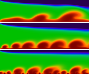
In figure 3, we plot the effect of different dimensionless Debye lengths  ${\lambda _D}$ on the flow state under a fixed voltage difference
  $\Delta \phi = 40$. Upon decreasing the dimensionless Debye length
  ${\lambda _D}$, massive small-scale vortices are ejected near the cation permselective membrane, forming an irregular concentration boundary layer structure. These figures imply that the flow chaos is not only affected by the well-known voltage difference
  $\Delta \phi $ but is also significantly modulated by the dimensionless factor
  ${\lambda _D}$. The periodic-to-chaotic transition is determined from the delay-time phase diagram, which has been successfully used to identify the flow states (Kwak et al. Reference Kwak, Pham and Han2017). To quantitatively describe fluid chaos, velocity attractors are adopted in a time-delay phase space. The velocity spatiotemporal fluctuation curves at a point
  $(x,y) = (2.5,\;{y_{ESC}})$ at the edge of the ESC layer and the slip velocity attractors
  $[u(t + \tau ),u(\tau )]$ in a time-delay phase space are presented in figures 2(b) and 2(c), respectively. Here,
  $\tau $ is the time delay. These attractors clearly reveal that reducing
  ${\lambda _D}$ can cause the flow to move from a steady state to a chaotic state.

Figure 3. Effect of the dimensionless parameter  ${\lambda _D}$ on the fluid state. (a) Surface instantaneous snapshots show the fully developed salt concentration for various
  ${\lambda _D}$. The blue colours show the ion enrichment regime emerging from the top cation permselective membranes, while the red colours show the depletion vortices formations near the bottom cation permselective membranes. (b) Instantaneous velocity profiles at the monitoring points
  $(x,y) = (2.5,\; {y_{ESC}})$ for various
  ${\lambda _D}$. (c) Slip velocity attractors in a time-delay phase space. As the dimensionless Debye length
  ${\lambda _D}$ decreases, the velocity fluctuation of the ESC layer becomes more chaotic, indicating that
  ${\lambda _D}$ can significantly regulate the flow state. The local small-scale vortices
  ${d_s}$ need to be magnified several times for viewing. Here,
  $\Delta \phi = 40$ and
  ${U_{HP}} = 240$.
At the small dimensionless Debye length  ${\lambda _D}$ scenario, we identify a distinct transitional pathway to the chaotic state that does not feature the conventional chaos bursts (Kwak et al. Reference Kwak, Pham and Han2017) and instead proceeds via the characteristics of the ESC layer. Physically, decreasing the dimensionless Debye length can weaken the ESC layer thickness
  $(\lambda _D^{2/3})$ and enhance the electrostatic driving force
  $({\nabla ^2}\phi \boldsymbol{\nabla }\phi \sim {\phi ^2}/d_{EC}^3)$, resulting in small-scale vortices erupting. These small-scale vortices interact in a complicated manner through the shear flow, which eventually leads to fluid chaos. As a result, the slip velocity increases with decreasing dimensionless Debye length
  ${\lambda _D}$. Consequently, a transition to flow chaos can occur via two distinctly different pathways, namely, (i) through increasing the voltage difference
  $\Delta \phi $ (Kwak et al. Reference Kwak, Pham, Lim and Han2013a,Reference Kwak, Guan, Peng and Hanb, Reference Kwak, Pham and Han2017) and (ii) through decreasing the dimensionless Debye length
  ${\lambda _D}$ (see figure 3). This implies that the fluid state is regulated by the combination of voltage difference
  $\Delta \phi $ and dimensionless Debye length
  ${\lambda _D}$ at a fixed shear flow velocity. Even though the pathways to the chaotic state can be different, there may be a universal criterion, the critical slip velocity of the vortex. Next, for a fixed shear flow velocity scenario, based on the DNS and scaling, we explore how the dimensionless Debye length
  ${\lambda _D}$ and voltage difference
  $\Delta \phi $ jointly regulate the flow state and slip velocity.
3.2. Slip velocity for the shear vortex
For a microfluidic system with permselective membranes, the critical factor of the flow state is recommended at a fixed shear flow velocity scenario. Our analysis has shown that increasing the voltage difference  $\Delta \phi $ or decreasing the dimensionless Debye length
  ${\lambda _D}$ can enhance the chaos and slip velocity. It is well known that the slip velocity
  ${u_s}$ at the edge of the ESC layer is the most basic driving factor that drives the vortex to roll. Consequently, the slip velocity
  ${u_s}$ is expected to yield a quantitative understanding of the selection of the flow state. Using the scaling
  ${(\lambda _D^{ - 1}\Delta {\phi ^4})^{1/3}}$, we found that the scattered data in figure 4(b) all collapse on a straight line,
 \begin{equation}{u_s} = \alpha \cdot {(\lambda _D^{ - 1}\Delta {\phi ^4})^{1/3}}.\end{equation}
Here, the theoretical analysis is performed for the configuration with a fixed shear flow velocity  ${U_{HP}} = 240$. In this scenario, the fitting coefficient
  $\alpha $ is 0.12. Figure 4(a) supports the reliability of our scaling analysis. Further analysis of the slip velocity shows that the selection of the flow state can be distinguished by the critical value of slip velocity
  ${u_{cri}}$, and its value is approximately 210. The increase in the slip velocity can promote the overall growth of the vortex, forming a steady vortex structure with a regular charge layer, as shown in figure 4(b). With this fixed shear flow velocity, however, the slip velocity further reached a critical value (~210), the vortex became overwhelmed, and an irregular charge layer structure was formed. From this perspective, the critical slip velocity
  ${u_{cri}}$ is recommended as the critical selection factor for the steady and chaotic states. Based on the scaling
  ${u_s}\sim {(\lambda _D^{ - 1}\Delta {\phi ^4})^{1/3}}$, a lower voltage difference
  $\Delta \phi $ is required in the smaller
  ${\lambda _D}$ scenario for the chaotic state.

Figure 4. Slip velocity scaling. (a) Slip velocity of the vortex plotted against the scaling factor  ${(\lambda _D^{ - 1}\Delta {\phi ^4})^{1/3}}$. The data points are all extracted from figure 5(b). Here, the slip velocity
  ${u_s}$ is defined as the time average
  ${u_s} = (1/({t_1} - {t_0}))\int_{{t_0}}^{{t_1}} {\sqrt {{u^2} + {v^2}\,\textrm{d}t} } $ of the velocity at the edge of the ESC layer, where
  ${t_0}$ is the initial time and
  ${t_1}$ is the cut-off time after the EC flow is fully developed. (b) Snapshot plots show the ESC layer superimposed with streamlines. In the scenario of high slip velocity, the area corresponding to the red streamline at the edge of ESC layer (need to be enlarged to view), the membrane surface ejects the chaotic multilayer charge boundary layer structure. However, the slip velocity is below the critical slip velocity, forming a steady flow, which corresponds to the streamlined blue area in the bottom picture of figure 4(b). Here,
  ${U_{HP}} = 240$.

Figure 5. Joint regulation of the flow state and slip velocity by  ${\lambda _D}$ and
  $\Delta \phi $. (a) Critical selection of ECF from steady to chaotic state for phase diagram replotted in dimensionless numbers:
  $\Delta \phi $ versus
  ${\lambda _D}$. The black curve is expressed as the critical line,
  $\Delta \phi = {({u_{cri}}/\alpha )^{3/4}}\lambda _D^{1/4}$, which is calculated by scaling (3.1). For a larger
  ${\lambda _D}$, a larger voltage difference
  $\boldsymbol{\nabla }\phi $ can reach the chaotic state. (b) Effect of
  $\Delta \phi $ and
  ${\lambda _D}$ on the slip velocity. The blue dashed line marks the slip velocity threshold, above which the flow is chaotic. Here,
  ${U_{HP}} = 240$.
Based on the above numerical analysis, the slip velocity is recommended as a key factor for the critical selection of the flow state. Using the critical value of slip velocity  ${u_{cri}}$, the instability phase diagram related to
  ${\lambda _D}$ and
  $\Delta \phi $ is obtained (see figure 5a). In the scenario of a fixed shear flow, once the input parameters (
 ${\lambda _D}$ and
  $\Delta \phi $) of the system are above the critical line, the flow is chaotic. Our DNS data support this analysis (see figure 5b). Consequently, for a larger
  ${\lambda _D}$, a higher voltage difference is required for the flow to maintain the chaotic state since the driving force
  $- {\nabla ^2}\phi \boldsymbol{\nabla }\phi + \boldsymbol{\nabla }P$ of the ESC layer is smaller. From the perspective of the slip velocity, a larger slip velocity can lead to the onset of the chaotic state.
For real electrochemical systems, scaling (3.1) can be rewritten as an alternative form,  ${\tilde{u}_s}\sim \tilde{l}_0^{1/3}\Delta {\tilde{\phi }^{4/3}}$, which is jointly regulated by the key physical parameters of the system input. Increasing the channel height
  ${\tilde{l}_0}$ and voltage difference
  $\Delta \tilde{\phi }$ can enhance the instability. In fact, the channel height
  ${\tilde{l}_0}$ and the voltage difference
  $\Delta \tilde{\phi }$ can span several orders of magnitude, such as
  ${{O}}(10)[\mathrm{\mu }\textrm{m}] < {\tilde{l}_0} < O({10^3})[\mathrm{\mu }\textrm{m}]$ and
  ${{O}}(10)[\textrm{mV}] < \Delta \tilde{\phi } < O({10^3})[\textrm{mV}]$. More generally, voltage difference regulation is the most common strategy for enhancing flow chaos, appearing in many ECF studies (Demekhin et al. Reference Demekhin, Nikitin and Shelistov2013; Kwak et al. Reference Kwak, Pham, Lim and Han2013b, Reference Kwak, Pham and Han2017; Shelistov et al. Reference Shelistov, Demekhin and Ganchenko2014). Controlling the flow state is conducive to guiding the design of desalination systems and electrodeposition.
3.3. Critical shear velocity for the shear sheltering
For fluid control, applying external shear flow is a common method to suppress flow chaos and has recently been successfully used to control the ECF state (Kwak et al. Reference Kwak, Pham and Han2017). In this section, the results of § 3.2 are further extended to describe the critical parameter values of the flow state under various shear flow velocities. In figure 6(a), we plot the flow patterns at different shear flow velocities. Increasing the shear velocity  ${U_{HP}}$, the chaotic vortex is suppressed by the shear flow, forming a regular oblique structure. For larger shear flow velocities, a large voltage difference is required to trigger flow chaos, as shown in figure 6(a).

Figure 6. Shear sheltering. Surface instantaneous snapshots show the cation concentration field and flow field structure for different shear flow velocities. Increasing the shear flow velocity can shelter chaos, whereas increasing the voltage difference can enhance chaos. Flow states are identified by slip velocity attractors; see Appendix D. (b) Balance mechanism of velocity average intensity. (c) Linear relation between the shear flow velocity and the slip velocity. Here,  ${\lambda _D} = {10^{ - 3}}$.
Based on the shear limit criterion (Terry Reference Terry2000; Kwak et al. Reference Kwak, Pham and Han2017), the critical balance relation  ${U_{HPC}}/(1 - {\delta _c})\sim {u_s}/{\delta _c}$ between the average intensity of the shear flow velocity and the average intensity of the vortex slip velocity is obtained (see figure 6b). Consequently, the critical shear velocity and slip velocity satisfy an approximately linear relation
  ${U_{HPC}}\sim ((1 - {\delta _c})/{\delta _c}){u_s}$ but are disturbed by the prefactor coefficient
  $(1 - {\delta _c})/{\delta _c}$. However, previous studies suggested that the steady state and chaotic state can be distinguished by the critical thickness
  ${\delta _c}$ of the vortex boundary layer, and its value is 0.309 (Kwak et al. Reference Kwak, Pham and Han2017). This indicates that
  ${\delta _c}$ is basically fixed for shear sheltering. Ignoring the disturbance prefactor coefficient
  $(1 - {\delta _c})/{\delta _c}$, a simple linear scaling
  $({U_{HPC}}\sim {u_s})$ is obtained (see figure 6c). This approximately linear scaling is confirmed by DNS. Consequently, the chaotic state is characterized by high slip velocity, which indicates that a larger shear velocity is required to shelter chaos. By exploring the shear velocity and slip velocity under the parameter space (
 ${\lambda _D}$,
  $\Delta \phi $ and
  ${U_{HP}}$), one can further understand the critical shear velocity required for chaos suppression. Please refer to Appendix C for more details.
Based on the above theory and numerical analysis, the fluid state is adjusted by the dimensional Debye length  ${\lambda _D}$, shear velocity
  ${U_{HP}}$ and voltage difference
  $\Delta \phi $. As the scaling factor
  ${(\lambda _D^{ - 1}{\varDelta\phi ^4})^{1/3}}$ increases, the fluid state is dominated by electrostatic force, and fluid chaos is enhanced. However, increasing the shear velocity, the flow is dominated by the pressure flow, and the flow chaos is suppressed. Using the scaling relation
  ${U_{HPC}}\sim {u_s}$, a universal phase diagram for shear sheltering can be obtained. Hence, one can obtain the scaling of the critical shear velocity,
 \begin{equation}{U_{HPC}} = c \cdot {(\lambda _D^{ - 1}\Delta {\phi ^4})^{1/3}} + \xi .\end{equation}
For a given dimensional Debye length, the present parameter space ( ${10^{ - 6}} \le {\lambda _D} \le {10^{ - 2}}$,
  $240 \le {U_{HP}} \le 1000$ and
  $0 \le \Delta \phi \le 120$), the fitting coefficients are
  $c = 0.56$ and
  $\xi = 912.87$. Finally, the data in figures 4–6 and experimental data (Kwak et al. Reference Kwak, Pham and Han2017) are replotted in the phase diagram composed of
  ${(\lambda _D^{ - 1}\Delta {\phi ^4})^{1/3}}$ and
  ${U_{HP}}$. In figure 7, the two states of the flow are successfully distinguished by a theoretical straight line. This analysis is supported by DNS data and experimental data (Kwak et al. Reference Kwak, Pham and Han2017). In addition, note that an effective voltage difference
  $\Delta \phi = \gamma \varphi $ was introduced in multilayer electrodialysis, where
  $\Delta \phi $ is the voltage difference between the membrane,
  $\varphi $ is the total voltage in multilayer electrodialysis and
  $\gamma $ describes the resistance effect in multilayer electrodialysis. Therefore, the coefficient
  $\gamma $ is assumed to be 0.042 to consider the effective voltage difference caused by the resistance effect of multilayer electrodialysis. Once the shear flow velocity
  ${U_{HP}} > {U_{HPC}}$, the shear flow shelters the chaos. However, when
  ${U_{HP}} < {U_{HPC}}$, the electrostatic force destabilizes the steady flow.

Figure 7. Critical shear velocity for shear sheltering. Critical selection of ECF from steady to chaotic state for phase diagram replotted in dimensionless numbers:  ${(\lambda _D^{ - 1}\Delta {\phi ^4})^{1/3}}$ versus
  ${U_{HP}}$. The dimensionless Debye layer length
  ${\lambda _D}$ describes the effect of the ESC length (regulated by the dimensionless Debye layer length) on the flow state,
  $\Delta \phi$ depicts the effect of the voltage difference and the shear velocity
  ${U_{HP}}$ characterizes the shear shielding. For convenience, two regional colours are used to distinguish the flow state. The chaotic state is maintained by the large slip velocity, and a larger shear flow velocity is required to suppress the chaos. Here, we extracted all experimental data (Kwak et al. Reference Kwak, Pham and Han2017) under the dimensionless Debye length
  ${\lambda _D} = {10^{ - 6}}$ with various shear flow velocities [
 ${U_{HP}} = 207(2.5\;\mathrm{\mu }\textrm{l/min})$,
  ${U_{HP}} = 414(5\;\mathrm{\mu }\textrm{l/min})$,
  ${U_{HP}} = 828(10\; \;\mathrm{\mu }\textrm{l/min})$ and
  ${U_{HP}} = 1656(20\;\mathrm{\mu }\textrm{l/min})$].
4. Conclusion
In summary, for a given dimensional Debye length scenario, this work investigates the critical selection between the steady state and chaotic state in an overlimiting electrodialysis channel embedded with two permselective membranes. The main conclusions are as follows.
(i) The theoretical analysis shows that the flow state is adjusted by a new dimensionless factor, the channel height-dependent
 ${\lambda _D}$. In the overlimiting state, shear ECF usually has two states, including a stable state and a chaotic state. Decreasing ${\lambda _D}$ can enhance the electrostatic driving force, and many small-scale vortices are ejected near the membrane, resulting in a chaotic state.
(ii) In the scenario of fixed shear flow velocity, the scaling analysis and DNS find that the slip velocity is the direct cause of the switching between the stable and chaotic states. Based on the scaling law of critical slip velocity, the distinction between steady and chaotic states can be achieved.
(iii) For ionic fluid control by shear sheltering, the critical shear velocity relation
${U_{HPC}} = c{(\lambda _D^{ - 1}\Delta {\phi ^4})^{1/3}} + \xi $ is obtained. When the shear flow velocity is above the critical shear velocity ${U_{HPC}}$, the shear flow shelters the chaotic fluctuations, resulting in the transition of the flow from the chaotic state to the steady state. Existing experimental data (Kwak et al. Reference Kwak, Pham and Han2017) and our DNS results support the analysis.


These results allow one to quantitatively understand the fluid state and velocity statistics in the ECF and provide optimization guidance for the performance design of electromembrane microfluidic systems, such as desalination (Chuang et al. Reference Chuang, Diao, Huang, Huang, Senapati, Chang and Sun2020), mixing (Guan, Yang & Wu Reference Guan, Yang and Wu2021), preconcentration (Qiu et al. Reference Qiu, Gong, Li and Han2019), charge injection (Guan & Novosselov Reference Guan and Novosselov2019) and electrodeposition (Chen et al. Reference Chen, Zhu, Yan, Ju, Jiang and Wang2016; Zheng et al. Reference Zheng, Kim, Tu, Choudhury, Tang and Archer2020). In addition, our scaling analysis is performed on the case with the fixed dimensional Debye length, which is a limitation of the hypothetical scenario. Just for the non-shear electroosmotic flow, the effects of bulk concentration on the mixing efficiency (Peng & Li Reference Peng and Li2015), flow pattern (Aboelkassem Reference Aboelkassem2019; Tripathi et al. Reference Tripathi, Narla and Aboelkassem2020) and enrichment efficiency (Ouyang et al. Reference Ouyang, Ye, Li and Han2018) are investigated. Similarly, the concentration effect of the shear electroconvective flow may be interesting, and the experimental and theoretical studies on it deserve to be conducted in the future.
Acknowledgements
We also thank four anonymous reviewers for their insightful comments on the earlier draft of this paper.
Funding
This work is supported by the Natural Science Foundation of China (Grant Nos. 11972257 and 11802225) and the Natural Science Basic Research Plan in the Shaanxi Province of China (Program No. 2019JQ-261).
Declaration of interests
The authors report no conflicts of interest.
Appendix A. Stokes flow for electrokinetic microfluidics
ECF belongs to the low-Re-number flow, and the analysis of fluids based on the Stokes equation is a widely used simplified scheme (Davidson et al. Reference Davidson, Andersen and Mani2014; Druzgalski & Mani Reference Druzgalski and Mani2016; Liu et al. Reference Liu, Zhou and Shi2020c; Mani & Wang Reference Mani and Wang2020). The Stokes equation is adopted for the flow analysis in this paper. The corresponding simplification process is as follows. The dimensional form of the momentum equation is
 \begin{equation}{\tilde{\rho }_0}\frac{{\partial \tilde{\boldsymbol{U}}}}{{\partial \tilde{t}}} + {\rho _0}\tilde{\boldsymbol{U}}\boldsymbol{\cdot }\tilde{\boldsymbol{\nabla }}\tilde{\boldsymbol{U}} ={-} \tilde{\boldsymbol{\nabla }}\tilde{P} + \tilde{\mu }{\tilde{\nabla }^2}\tilde{\boldsymbol{U}} + \tilde{F}({\tilde{c}_ - } - {\tilde{c}_ + })\tilde{\boldsymbol{\nabla }}\tilde{\phi }.\end{equation}
To numerically solve these equations, the governing equations should be converted to the dimensionless form. Based on the dimensionless references in the main text, one can obtain the following dimensionless form of the Navier–Stokes equation,
 \begin{equation}\frac{1}{{Sc}}\frac{{\partial \boldsymbol{U}}}{{\partial t}} + Re\boldsymbol{U}\boldsymbol{\cdot }\boldsymbol{\nabla }\boldsymbol{U} ={-} {\nabla ^2}\boldsymbol{U} + \boldsymbol{\nabla }P - {\kappa _0}{\nabla ^2}\phi \boldsymbol{\nabla }\phi .\end{equation}
Here,  $Sc = \tilde{\mu }/{\tilde{\rho }_0}\tilde{D}$ is the Schmidt number and
  $Re = {\tilde{U}_0}{\tilde{l}_0}{\tilde{\rho }_0}/\tilde{\mu }$ is the Reynolds number. The definitions of the remaining parameters and symbols are listed in the main text.
Here, a simplified NS equation is used in the simulation. By ignoring the first two terms  $((1/Sc)(\partial \boldsymbol{U}/\partial t) + Re\boldsymbol{U}\boldsymbol{\cdot }\boldsymbol{\nabla }\boldsymbol{U})$ in (A2), it can be simplified to the Stokes equation,
 \begin{equation}{\nabla ^2}\boldsymbol{U} ={-} {\kappa _0}{\nabla ^2}\phi \boldsymbol{\nabla }\phi + \boldsymbol{\nabla }P.\end{equation}
The non-equilibrium ECF belongs to low-Reynolds-number and high-Schmidt-number flows. Therefore, the first two items  $((1/Sc)(\partial \boldsymbol{U}/\partial t) + Re\boldsymbol{U}\boldsymbol{\cdot }\boldsymbol{\nabla }\boldsymbol{U})$ in (A3) can be ignored in this study. By referring to the magnitude of the experimental parameters of the electrodynamic microfluidic device (Kwak et al. Reference Kwak, Pham and Han2017), the magnitude of the Re number and the Schmidt number of the ECF can be calculated as follows.
 \begin{gather}\left.
\begin{gathered} {Re =
{{\tilde{U}}_0}\dfrac{{{{\tilde{l}}_0}{{\tilde{\rho
}}_0}}}{{\tilde{\mu }}} = \dfrac{{{{10}^{ - 9}}\left[
{\dfrac{{{\textrm{m}^2}}}{\textrm{s}}}
\right]}}{{500\;[\textrm{mm}]}} \cdot 500\;[\textrm{mm}]
\cdot \dfrac{{{{10}^3}\left[
{\dfrac{{\textrm{kg}}}{{{\textrm{m}^3}}}}
\right]}}{{{{10}^{ - 3}}\;[\textrm{Pa} \cdot \textrm{s}]}}
= 0.001}\\ {Sc = \dfrac{{\tilde{\mu }}}{{{{\tilde{\rho
}}_0}{{\tilde{D}}_0}}} = \dfrac{{{{10}^{ -
3}}\;[\textrm{Pa} \cdot \textrm{s}]}}{{{{10}^3}\left[
{\dfrac{{\textrm{kg}}}{{{\textrm{m}^3}}}} \right] \cdot
{{10}^{ - 9}}\left[ {\dfrac{{{\textrm{m}^2}}}{\textrm{s}}}
\right]}} = 1000} \end{gathered} \right\}.\end{gather}
\begin{gather}\left.
\begin{gathered} {Re =
{{\tilde{U}}_0}\dfrac{{{{\tilde{l}}_0}{{\tilde{\rho
}}_0}}}{{\tilde{\mu }}} = \dfrac{{{{10}^{ - 9}}\left[
{\dfrac{{{\textrm{m}^2}}}{\textrm{s}}}
\right]}}{{500\;[\textrm{mm}]}} \cdot 500\;[\textrm{mm}]
\cdot \dfrac{{{{10}^3}\left[
{\dfrac{{\textrm{kg}}}{{{\textrm{m}^3}}}}
\right]}}{{{{10}^{ - 3}}\;[\textrm{Pa} \cdot \textrm{s}]}}
= 0.001}\\ {Sc = \dfrac{{\tilde{\mu }}}{{{{\tilde{\rho
}}_0}{{\tilde{D}}_0}}} = \dfrac{{{{10}^{ -
3}}\;[\textrm{Pa} \cdot \textrm{s}]}}{{{{10}^3}\left[
{\dfrac{{\textrm{kg}}}{{{\textrm{m}^3}}}} \right] \cdot
{{10}^{ - 9}}\left[ {\dfrac{{{\textrm{m}^2}}}{\textrm{s}}}
\right]}} = 1000} \end{gathered} \right\}.\end{gather}
To further confirm that this simplified theory is reasonable, the comparison of the numerical simulation results of the flow field structure is given based on the Navier–Stokes equation (A2) and the simplified Stokes equation (A3), as shown in figure 8. From the streamline (black line) and ion concentration distribution in figure 8, the Stokes equation (A3) can well capture the flow behaviour.

Figure 8. Snapshots of the dimensionless salt concentration with flow streamlines superposed for λ = 5 × 10⁻⁴. (a) DNS results based on the NS-PNP model; (b) DNS based on the Stokes-PNP model.
Appendix B. Effect of membrane concentration on the slip velocity
For simplicity, many physicists have introduced the boundary condition of a fixed dimensionless cation concentration at the membrane surface as  ${c_m} = 2$ (Rubinstein et al. Reference Rubinstein, Manukyan, Staicu, Rubinstein, Zaltzman, Lammertink, Mugele and Wessling2008; Demekhin et al. Reference Demekhin, Nikitin and Shelistov2013; Druzgalski et al. Reference Druzgalski, Andersen and Mani2013). The boundary condition of different given values of the membrane concentration is also considered in ECF (Green Reference Green2020). Here, the effect of different values of membrane concentration
  ${c_m}$ on the ECF is discussed. Through DNS, the effect of membrane concentration on flow is analysed, including the flow pattern, slip velocity and extended space charge layer. In figure 9, although the spatiotemporal evolution of the flow pattern is modulated by the membrane concentration, the spatiotemporal average of the vortex slip velocity has not yet been affected. In figure 9, although the spatiotemporal evolution of the flow pattern is modulated by the membrane concentration
  ${c_m}$, the average of the vortex slip velocity has not yet been affected. Since the slip velocity of the vortex originates from the electrostatic force at the edge of the ESC layer, it does not depend on the external shear flow. Therefore, the slip velocity of the vortex is closely related to the thickness of the ESC layer. In figure 9(c), the distribution of the ECS layer at different membrane concentrations is analysed. It is shown that the thickness of the ESC layer is independent of the membrane concentration
  ${c_m}$, which implies that the slip velocity is independent of the membrane concentration under the situation of statistical stationarity (see figure 9b). However, the membrane concentration only modulates the value of the charge density in the EDL, which leads to some differences in the spatiotemporal evolution of the vortex pattern. Our scaling shows that the ESC layer thickness satisfies the scaling relation,
  $\lambda _D^{2/3}\phi _{ESC}^{2/3}{j^{ - 1/3}}$. This indicates that the membrane concentration is independent of the ESC thickness, and therefore, the time average of the slip velocity is independent of the membrane concentration, as shown in figure 9(b).

Figure 9. Effect of membrane concentration on flow. (a) Effect of membrane concentration on the flow pattern at  $\Delta \phi = 60$. (b) Average slip velocity at different membrane concentrations and voltage differences. (c) ESC layer distribution at different membrane concentrations. Here,
  ${\lambda _D} = {10^{ - 3}}$ and
  ${U_{HP}} = 240$.
Appendix C. Analysis of the shear velocity and slip velocity
Figure 10(a) presents the flow patterns under two sets of shear velocities, the spatiotemporal fluctuations of the slip velocity and the slip velocity attractors. It is shown that the time averaging of slip velocity is almost independent of shear flow but that vortex height and velocity fluctuations can be adjusted. Therefore, an increase in shear flow velocity can suppress the flow disturbance but hardly affect the spatiotemporal average of the slip velocity, since the slip velocity originates from the electrostatic force at the edge of the expanding space charge layer, rather than the external shear flow. In figure 10(b), the time-averaged speeds are 260 and 265, and this slight change can be ignored.

Figure 10. Effect of shear velocity on flow. Shear flow velocity modulates (a) flow pattern, (b) spatiotemporal fluctuations and (c) velocity attractors. Here,  ${\lambda _D} = {10^{ - 3}}$ and
  $\Delta \phi = 60$.
We also count the slip velocities at various shear flow velocities, as shown in figure 11. As the shear flow velocity increases, the critical voltage for triggering the chaotic state is higher. For a fixed shear flow velocity, the critical slip velocity required for the chaotic state is universal. When the shear flow velocity is set to 240, a critical slip velocity (~210) is required to trigger flow chaos; see figure 11(a). As discussed in the main text, the slip velocity is also affected by the dimensionless Debye layer length. Although reducing the dimensionless Debye layer length can enhance the slip velocity and flow chaos, the slip velocity required for the flow to enter the chaotic state is universal, at approximately 210; see figures 3 and 4. In figure 11, the shear flow velocity increases further, and the onset voltage of the flow chaos increases. Once the shear ECF is dominated by electrostatic forces, the electrostatic force destabilizes the steady flow.

Figure 11. Slip velocity for (a)  ${U_{HP}} = 240$, (b)
  ${U_{HP}} = 600$ and (c)
  ${U_{HP}} = 800$. An increase in shear flow velocity results in a higher onset voltage of flow chaos. Here,
  ${\lambda _D} = {10^{ - 3}}$.
The scaling (3.1) suggests that the slip velocity is regulated by the dimensionless Debye layer length  ${\lambda _D}$. The scaling coefficient
  $\alpha = 0.12$ is confirmed to be independent of the shear flow velocity. In figure 13(a), we analyse the effect of shear flow velocity on slip velocity for the dimensionless Debye layer length (λ D = 5 × 10⁻⁴) scenario. For the larger shear flow velocity scenario
  ${U_{HP}} = 1000$, there is a slight change in the slip velocity. Using the scaling
  $0.12 {(\lambda _D^{ - 1}\Delta {\phi ^4})^{1/3}}$, it is found that the scattered data in figures 11 and 12(a) all collapse on a straight line, as shown in figure 12(b). These analyses show that in the present parameter space,
  $0.12 {(\lambda _D^{ - 1}\Delta {\phi ^4})^{1/3}}$ can basically reveal the evolution law of slip velocity. That is, the fitting coefficient
  $\alpha = 0.12$ is independent of the shear velocity.

Figure 12. Slip velocity. (a) Effect of  $\Delta \phi $ and
  ${\lambda _D}$ on the slip velocity. (b) Scaling behaviour of the slip velocity. The slip velocity of the vortex is plotted against the scaling
  $0.12 {(\lambda _D^{ - 1}\Delta {\phi ^4})^{1/3}}$, which shows that the coefficient
  $\alpha = 0.12$ is independent of the shear flow velocity
  ${U_{HP}}$ in the present parameter space.

Figure 13. Slip velocity attractors in a time-delay phase space for (a)  ${U_{HP}} = 240$, (b)
  ${U_{HP}} = 800$ and (c)
  ${U_{HP}} = 1000$. Based on these delay time phase diagrams, the flow state of figure 6(a) in the main text is determined. Here,
  $\; {\lambda _D} = {10^{ - 3}}$.
Appendix D. The attractors in a time-delay phase space
To identify the flow states in figure 13(a), the attractors in a time-delay phase space (Kwak et al. Reference Kwak, Pham and Han2017) are used. By analysing the attractor of slip velocity to identify the transition from chaotic to stable flow, one can quantitatively describe how the transition from chaotic sequence to periodic sequence of slip velocity is caused by shear flow. The time series of slip velocities are recorded to fix a point at the edge of the ESC layer, and delay time phase diagrams of these time series are plotted to determine the flow state of figure 6(a), as shown in figure 13.


