3. Results and discussion

Three experimental runs (corresponding to cases 1–3) are performed in this work. Initial conditions are listed in table 1. The Atwood number ( $A$ ) is defined as $A = (\rho _2 - \rho _1)/$ $(\rho _2 + \rho _1)$ with $\rho _1$ ( $\rho _2$ ) being the gas density on the exterior (interior) side of the interface, and the mass fraction of SF $_6$ is calculated based on one-dimensional (1-D) gas dynamics theory. The main steps for converting PLIF images from intensity to mole fraction are outlined below. First, the distortion caused by the camera system is corrected using a circular calibration plate. Next, background images (taken without the injection of the SF $_6$ and acetone mixture into the test section) are subtracted from the PLIF images. Then, the divergence and spatial variation of the laser sheet are taken into account. Also, Beer’s law attenuation is iteratively calibrated under the assumption of adiabatic mixing. Finally, a notch filter is applied to remove striations caused by interface refraction. After this process, the mole fraction of the gas mixture, rather than just SF $_6$ , enclosed by the interface is obtained.

Table 1. Initial conditions for cases 1–3. $Ma$ : Mach number of the incident shock when it arrives at the interface; $R$ : radius of initial interface; $h_0$ : initial width of the mixing layer; mfra(SF $_6$ ): SF $_6$ mass fraction; $A$ : Atwood number; $\chi _{\textit{acetone}}$ : acetone volume fraction.

The initial interface formed in the present experiments is relatively sharp, enabling the extraction of the isoline where the mole fraction of the interior gas is 0.5, as depicted in figure 2(a ), where the dash-dotted lines represent the average position of the initial interface. The perturbations in cases 1 and 3 are nearly identical, which explains the similar growth rate of mixing width observed later. In contrast, the amplitude of case 2 is relatively smaller, but its phase aligns with those of cases 1 and 3. For spherical RM instability, spherical harmonics are typically employed to initialize interfacial perturbations, as they effectively avoid the pole singularity problem on a spherical interface (Lombardini, Pullin & Meiron Reference Lombardini, Pullin and Meiron2014). However, for RM instabilities in cylindrical geometries, which are simpler than spherical geometries, a linear superposition of Fourier harmonics is more commonly recommended (Ge et al. Reference Ge, Zhang, Li and Tian2020). In the present experiments, the initial interface is measured on a 2-D plane using PLIF diagnostics, and thus the amplitude of the initial perturbations can be expanded as

(3.1) \begin{equation} f\left ( \theta \right ) =\sum _{m=0}^N{f_me^{ik_mR\theta }}, \end{equation}

where the amplitude coefficients $f_m$ are determined by the variance $\sigma _{m}^{2}= ({1}/{2\pi })(({P ( k_m )}/{k_m}))\varDelta k$ with $P (k_m )$ being the power spectrum. Figure 2(b ) displays the power spectra of the initial perturbations for cases 1–3. It is evident that the retractable plate generates a specific multi-mode perturbation characterized by small amplitudes across a broad range of high wavenumbers. The perturbation spectrum exhibits an approximate scaling law of -4/3, similar to observations in ICF capsules (Barnes et al. Reference Barnes2002).

Figure 2. (a) The radial position of the initial interface plotted against the azimuthal angle. The dash-dotted lines indicate the average position of the initial interface. (b) The power spectra of the initial perturbations. The black line serves as a reference for a scaling law.

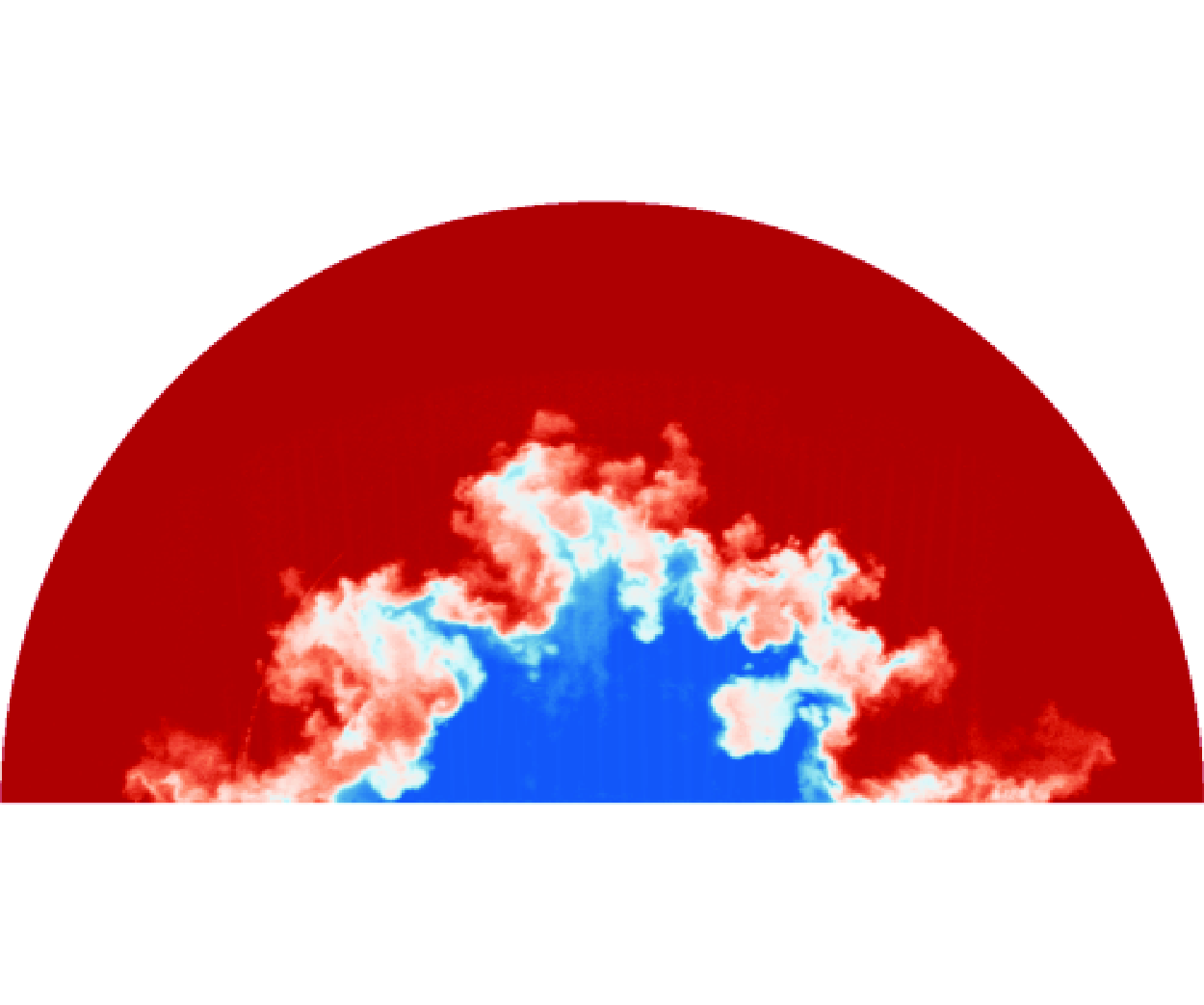
Figure 3. Temporal evolutions of mole fraction distribution for cases 1–3. II, initial interface; SI, shocked interface; TS, transmitted shock; RTS, reflected transmitted shock; RI, reshocked interface. Numbers at the top left of the images in the first column are in time (unit: ms).

Evolutions of mole fraction field for cases 1–3 are displayed in figure 3. Time origin is set at the moment when the incident shock encounters the interface. The first row of images illustrates the initial interface, while the second row displays the interface after the shock impact. Fine-scale interface structures at every stage are clearly captured by the PLIF diagnostic. Unlike previous experiments, the interface here maintains a distinct and sharp morphology during both the linear and nonlinear stages, indicating the elimination of diffusion layer on the initial interface formed. Moreover, large-scale perturbations along the cylinder axis caused by the retracting plate are effectively excluded in the present experiments. According to our previous study (Ding et al. Reference Ding, Si, Chen, Zhai, Lu and Luo2017a ), if large-scale perturbations are present along the cylinder axis, the longitudinal interface will evolve rapidly with the roll-up of vortices following shock impact, resulting in significant mutual penetration of flow structures between planes perpendicular to the cylinder axis. However, the present experimental results show no such mutual penetration, providing evidence against the presence of large-scale perturbations. As the shocked interface moves inward, the short-wavelength perturbations produced by the retracting plate grow rapidly. Later, the transmitted shock focuses at the convergence centre, immediately generating a diverging reflected shock (0.27 ms). Subsequently, this reflected shock re-impacts the evolving interface, leading to a rapid transition to turbulent mixing ( $t\gt$ 0.59 ms). The laminar boundary layer in the post-shock flow has a maximum thickness of 0.11 mm, indicating that it has a negligible influence on the interface development. If the laminar boundary layer transitions to turbulence after reshock (similar to the main flow), the turbulent boundary layer is not expected to be an order of magnitude thicker than the laminar boundary layer (i.e. 1.1 mm) during the short experimental period. The PLIF diagnostic captures the flow information at the centre plane of the test section (2.5 mm from either wall). Therefore, the flow field captured by PLIF cannot be significantly affected by the boundary layer.

An $r{-}t$ diagram illustrating the trajectories of the interface and shock waves is given in figure 4(a ). The wave motions are calculated with 1-D gas dynamics theory, which can approximately represent the actual shock propagation process. The interface position is extracted from the mole fraction image where $\left \lt \xi \right \gt =0.5$ , with $\left \lt \cdot \right \gt$ denoting the circumferential averaging. In general, the interface trajectories for cases 1–3 are similar. Impacted by the incident shock, the interface moves inwards at an initial velocity of approximately 110.0 m s^–1. Then, it experiences evident deceleration, consistent with previous schlieren results (Ding et al. Reference Ding, Si, Yang, Lu, Zhai and Luo2017b ). Following reshock, the interface first undergoes a short period of outward motion, then decelerates and even moves inwards gradually due to mass conservation of the fluid enclosed by the interface. This confirms the numerical results of Lombardini et al. (Reference Lombardini, Pullin and Meiron2014). Visible oscillations in the interface trajectory are observed, which is ascribed to the subsequent waves reverberating between the interface and geometric centre.

Figure 4. (a) Trajectories of the interface and shock waves and (b) the mixing layer width vs. time for cases 1–3. Dashed lines in (b) indicate the linear fits of data. IS, incident shock; TS $_2$ , second transmitted shock. The other symbols are the same as those in figure 3.

The growth of the mixing layer width is plotted in figure 4(b ). The mixing width is defined as $h=r_s-r_b$ with $r_s$ being the radius where the average mole fraction of heavy gas $\left \lt \xi \right \gt =0.05$ and $r_b$ being the radius where $\left \lt \xi \right \gt =0.95$ . After the incident shock impact, the mixing width exhibits a rapid growth ( $t\lt 0.2\,\rm ms$ ). Later, the growth rate suffers a continuous drop and even becomes negative due to the RT stabilization effect caused by interface deceleration (Ding et al. Reference Ding, Si, Yang, Lu, Zhai and Luo2017b ). After reshock, the mixing width first suffers a sudden drop due to shock compression, then presents a period of quasi-linear growth with time. Such a quasi-linear growth is qualitatively consistent with the behaviour of reshocked RM instability in planar geometry (Leinov et al. Reference Leinov, Malamud, Elbaz, Levin, Ben-Dor, Shvarts and Sadot2009). Mikaelian (Reference Mikaelian1989) has proposed an empirical model to predict the mixing width growth for RM turbulence

(3.2) \begin{equation} \frac {\mathrm {d}h}{\mathrm {d}t}=C_M\Delta V\left | A_{r}^{+} \right |, \end{equation}

where $\Delta V$ is the interface jump velocity caused by reshock, $A_{r}^{+}$ is the post-reshock Atwood number and $C_M$ is an empirical coefficient. Performing a linear fit of the present data, $C_M$ is found to be 0.99, 0.83 and 0.98 for cases 1–3, respectively. Note that $C_M$ = 0.28 is suggested by Mikaelian (Reference Mikaelian1989), and $C_M = 0.28{\sim}0.39$ is suggested by experiments on planar RM instability with reshock (Leinov et al. Reference Leinov, Malamud, Elbaz, Levin, Ben-Dor, Shvarts and Sadot2009). This means that the present growth rate in the convergent geometry is more than twice the rate in planar RM turbulence. The explanation is as follows. The interface experiences unsteady motion in a convergent geometry, triggering RT instability or stability, which may be a key factor for the quicker growth of perturbations. As we know, the RT instability occurs when the acceleration vector is directed from a light fluid toward a heavy fluid. To identify these periods in our experiment, we calculate the interface acceleration by taking the second derivative of the interface trajectory given in figure 4(a ). While our experimental time resolution limits precise quantification of instantaneous interface acceleration, qualitative analysis reveals that, following reshock ( $t\gt 0.35\,\rm ms$ ), the outward-moving interface experiences deceleration due to mass conservation of the fluid enclosed by the interface. This deceleration triggers RT instability, which remains active until $t=0.83\,\rm ms$ , coinciding with the period of rapid quasi-linear growth observed in figure 4(b) between 0.43 and 0.83 ms. Additionally, geometric contraction enhances instability growth at an inward-moving interface, leading to a larger perturbation amplitude prior to reshock. This can also contribute to faster instability growth after reshock. Furthermore, unlike in previous planar experiments, the interface here lacks a diffusion layer, allowing it to retain a sharper morphology at the reshock moment. As noted by Ukai, Balakrishnan & Menon (Reference Ukai, Balakrishnan and Menon2011), in such cases, more baroclinic vorticity is generated at the interface, further accelerating the instability growth. It is also found that, unlike the planar counterpart, the mixing width here does not exhibit a power-law growth at late stages. One major reason for this discrepancy is that the geometric centre restricts the mixing width growth. Also, subsequent waves reverberating between the interface and geometric centre also influence the mixing width growth.

The normalized mixed mass, defined as $\varPsi = ({\int {\langle \rho \xi ( 1-\xi ) \rangle {\rm d}r})}/({\int {\langle \rho\rangle \langle \xi \rangle \langle 1-\xi \rangle {\rm d}r})}$ (Zhou, Cabot & Thornber Reference Zhou, Cabot and Thornber2016), is calculated to quantify the mixing degree within the mixing zone. Here, $\varPsi =1$ represents a homogenized molecular mixing, while $\varPsi =0$ represents a completely entrained flow. As seen in figure 5(a), there exists only a minor difference among the three cases, demonstrating high reproducibility of the present experiments. After the shock impact, $\varPsi$ experiences a rapid decay due to the growth of the mixing width. Later, RT stabilization effect begins to act, which suppresses the mixing width growth (i.e. erases the large-scale intrusion between the two gases), leading to a continuous rise in $\varPsi$ . It is seen that $\varPsi$ reaches a peak at the time of reshock. After reshock, nonlinearity becomes strong and bubble merging dominates the instability development, generating shorter-wavelength structures (see figure 3). This process leads to a continuous drop of the mixedness parameter to a valley. At late stages, turbulent transport becomes strong, causing $\varPsi$ to rise to the range 0.8–0.9. Other mixedness parameters including molecular mixing fraction $\varTheta$ and mixing parameter $\varXi$ (Cook & Dimotakis Reference Cook and Dimotakis2001) are also calculated, and they present a similar variation trend as $\varPsi$ .

Figure 5. (a) Variations of mixedness with time for cases 1–3 and (b) the scalar energy spectra at times after reshock for case 1.

The scalar energy spectra at moments after reshock are given in figure 5(b ). They are calculated as follows. First, scalar fluctuations are obtained as $\xi ^*=\xi -\left \lt \xi \right \gt$ . Then, these fluctuations are Fourier transformed and multiplied by their Fourier conjugates to derive the scalar energy spectrum across different radii

(3.3) \begin{equation} E\left (k\right )=F\left (\xi ^\ast \right )F^{conj}\left (\xi ^\ast \right ). \end{equation}

Finally, the scalar energy spectrum is obtained by spatially averaging within the inner mixing zone. It is important to note that the limited height of the test section introduces geometric constraints that become significant as the mixing width approaches the test section height. This confinement effect is characterized by the suppression of vortex stretching due to the narrow test section height, which potentially causes an inverse transfer of energy from small to large scales (Thornber & Zhou Reference Thornber and Zhou2015). However, as depicted in figure 5(b ), immediately following reshock, only a minor amount of energy is transferred to the long-wavelength region (between 0.43 and 0.75 ms). Subsequently, the scalar energy in the long-wavelength region undergoes a continuous decay, indicating the dominance of energy transfer to smaller scales in the present experiments. This phenomenon explains the sustained increase in mixedness observed at later stages in figure 5(a ). Additionally, a distinctive feature of 2-D turbulence is the presence of an inertial subregion with a –3 scaling law at high wavenumbers (Boffetta & Ecke Reference Boffetta and Ecke2012). In contrast, the present results exhibit an inertial subrange with a $-7/3$ power law. According to Noble et al. (Reference Noble, Ames, McConnell, Oakley, Rothamer and Bonazza2023), for planar RM turbulence with $Sc=0.7$ (the Schmidt number in the present experiments), the power-law slope ranges between $-2.0$ and $-2.5$ . The similarity between the present power-law slope and the planar counterpart suggests that the dynamics of small scales is not fundamentally affected by the limited test section and the layer’s curvature. It is noteworthy that the scalar energy spectrum after reshock undergoes a slight change and displays a partial temporal similarity, but lacks strict self-similarity due to reverberating waves and geometric constraints. This behaviour, also observed in planar reshock RM turbulence (Tritschler et al. Reference Tritschler, Olson, Lele, Hickel, Hu and Adams2014), is interpreted as the rapid destruction of the initial conditions and large-scale structures following reshock. The present analysis indicates that although geometric constraints influence the flow evolution, they do not fundamentally alter the underlying mixing dynamics.

Figure 6. Evolutions of (a) turbulent length scales and (b) Reynolds numbers.

Turbulent length scales are measured within the mixing zone based on the mole fraction field. Because the turbulent length scales of cases 1–3 are similar, only the results for case 1 are shown here (the remaining results can be found in the Supplemental file). The Taylor microscale is calculated by $\lambda _T=\sqrt {\lambda _{T,r}^{2}+\lambda _{T,\theta }^{2}}$ with the radial Taylor microscale $\lambda _{T,r}$ and the circumferential Taylor microscale $\lambda _{T,\theta }$ obtained from the spatial variance and gradients of the mole fraction fluctuation (Pope Reference Pope2000). The Liepmann–Taylor scale, $\lambda _L$ , is estimated based on the Taylor microscale as $\lambda _L \simeq 2.17\lambda _T$ (Dimotakis Reference Dimotakis2000). The Batchelor scale $\lambda _B$ cannot be obtained directly from experiment due to the limited image resolution, and is estimated from the dissipation layer thickness, i.e. $\lambda _{20\,\%} \simeq 5.0\lambda _B$ (Weber et al. Reference Weber, Haehn, Oakley, Rothamer and Bonazza2014). In this work, $\lambda _{20\,\%}$ is calculated from the scalar dissipation rate field, representing the characteristic dissipation scale with the highest probability density. Since the Schmidt number $Sc \approx 0.7$ in the present experiments, $\lambda _B$ is nearly equivalent to the Kolmogorov scale. Thus, the inner viscous scale, $\lambda _{\nu }$ , can be estimated based on Batchelor scale as $ \lambda _{\nu } \simeq 50\lambda _B$ . For evaluating the flow transition, Dimotakis (Reference Dimotakis2000) has proposed a criterion: $\lambda _L/\lambda _{\nu }\gt 1$ . Later, Zhou et al. (Reference Zhou, Robey and Buckingham2003b ) proposed a new transition criterion, $\min ( \lambda _D, \lambda _L ) \gt \lambda _{\nu }$ , for unsteady flow transition which additionally requires a sufficiently long evolution time. Here, the diffusion layer scale is $\lambda _D=5 ( \nu t ) ^{1/2}+W_{0}^{r+}$ , with $\nu$ being the kinematic viscosity and $W_{0}^{r+}$ being the post-reshock mixing width (Groom & Thornber Reference Groom and Thornber2021). As shown in figure 6(a ), both $\lambda _L$ and $\lambda _D$ are slightly larger than $\lambda _{\nu }$ after reshock, indicating the establishment of an inertial subrange (i.e. the occurrence of mixing transition) after reshock. The present result illustrates that reshock causes a rapid flow transition to turbulent mixing by enhancing the scale separation.

The transition criterion in terms of Reynolds number is $Re\gt 1-2\times 10^4$ (Dimotakis Reference Dimotakis2000). An outer-scale Reynolds number is calculated based on scale separation: $\lambda _L/\lambda _{\nu }= ({1}/{10})Re_1^{1/4}$ . Another definition of outer-scale Reynolds number is $Re_2=h\dot {h}/\nu$ . Notably, $Re_2$ is larger than $Re_1$ , as $Re_2$ is more sensitive to the evolution of large-scale structures, while $Re_1$ , calculated on the turbulent integral scale, remains largely unaffected. As plotted in figure 6(b ), both Reynolds numbers experience a rapid growth after reshock. This observation is consistent with the enhancement of scale separation caused by reshock. The present finding explains the quick transition after reshock seen in both previous and current experiments. It is found that both $Re_1$ and $Re_2$ are greater than $1\times 10^4$ after reshock, indicating that the transition criterion of Dimotakis (Reference Dimotakis2000) is also suitable for the convergent RM turbulence. One physical explanation is that small turbulent scales cannot feel the effect of geometric curvature.

Figure 7. Scaling-law exponents of $p$ -order structure functions.

The scaling-law exponents of the $p$ -order structure functions, defined as $S_p ( r_{\theta } ) =\left \lt ( \left | \xi ( x+r_{\theta } ) -\xi ( x ) \right | ) ^p \right \gt$ , at moments after reshock for case 1 (results for cases 2 and 3 can be found in the Supplemental file), are depicted in figure 7, where the Kolmogorov–Obukhov–Corrsin (KOC) exponent $\zeta _p=p/3$ is also provided for comparison. The exponents are obtained by linearly fitting the experimental data (see inset of figure 7) near Taylor microscale. For a short time after reshock (0.43 ms), the low-order exponents match the KOC prediction well, while the high-order ones present an evident discrepancy. As time progresses, the exponent of each order structure function increases, which we interpret as an indication of RM turbulence decay. Specifically, following reshock, fluid mixing becomes more homogeneous and thus turbulent fluctuations are reduced, especially at smaller scales, resulting in larger structure function exponents. Kraichnan (Reference Kraichnan1994) proposed an anomalous scaling theory, given by $\zeta _p={1}/{2}\sqrt {6p ( 2-\zeta ) + ( 1+\zeta ) ^2}- (({1}/{2}) ( 1+\zeta ))$ , where the parameter $\zeta$ ranges from 0 to 2. The present data match well with Kraichnan’s theory provided appropriate values of $\zeta$ . It is found that flow homogenization correlates with an increased $\zeta$ parameter, reflecting the physical meaning of the model. While Kraichnan’s theory was developed for isotropic turbulence at very high Reynolds numbers, there are several important considerations that support the partial applicability of this theory to our case. First, the RM turbulence, although globally inhomogeneous and anisotropic, exhibits local isotropy in the mixing plane perpendicular to the shock propagation direction (Zhou Reference Zhou2001; Zhou et al. Reference Zhou, Remington, Robey, Cook, Glendinning, Dimits and Eliason2003a ). This local isotropy provides a basis for applying theories developed for isotropic turbulence. Second, during turbulent transition in RM instability, a significant decoupling occurs between the energy-containing range and the dissipation range, establishing an inertial subrange. This decoupling reduces Reynolds number dependence, although higher Reynolds numbers do yield a broader inertial subrange (Dimotakis Reference Dimotakis2000; Zhou et al. Reference Zhou, Clark, Clark, Gail Glendinning, Aaron Skinner, Huntington and Remington2019). Despite these, we acknowledge the necessity of cautious interpretation of these comparisons due to the fundamental differences between idealized homogeneous isotropic turbulence (HIT) and the experimental conditions in our study.

The PLIF diagnostics can only capture 2-D data, and thus the energy spectrum and structure function reported in this work are calculated in a direction parallel to the mixing layer rather than using 3-D data. This raises the question of whether turbulent fluctuations in the spanwise direction differ statistically from those in the azimuthal direction. As far as we know, this issue has not been addressed through experiments since measuring the flow in the spanwise direction is challenging. However, previous numerical studies (Ge et al. Reference Ge, Zhang, Li and Tian2020) on convergent RM turbulence have shown that after reshock, the azimuthal and spanwise energy spectra become nearly identical, as the reflected shock can effectively eliminate initial interface features. This supports the analyses in this work.