


1 Introduction
Rayleigh–Bénard convection (RBC) is one of the simplest and most widely investigated models representing buoyancy-driven convection in geophysical, astrophy sical and industrial problems (Ahlers, Grossmann & Lohse Reference Ahlers, Grossmann and Lohse2009; Lohse & Xia Reference Lohse and Xia2010). In addition to the scaling between the Nusselt and Reynolds numbers, which is successfully explained by Grossmann–Lohse (GL) theory (Grossmann & Lohse Reference Grossmann and Lohse2000, Reference Grossmann and Lohse2001, Reference Grossmann and Lohse2002; Ahlers et al. Reference Ahlers, Grossmann and Lohse2009; Lohse & Xia Reference Lohse and Xia2010), the reversals of large-scale circulation (LSC) in RBC are also interesting and have been investigated intensively (Benzi Reference Benzi2005; Brown & Ahlers Reference Brown and Ahlers2007, Reference Brown and Ahlers2008b; Assaf, Angheluta & Goldenfeld Reference Assaf, Angheluta and Goldenfeld2011; Petschel et al. Reference Petschel, Wilczek, Breuer, Friedrich and Hansen2011; Vasil’ev & Frick Reference Vasil’ev and Frick2011; Wagner & Shishkina Reference Wagner and Shishkina2013). In cylindrical geometry, the reversals can be caused by azimuthal rotations of the LSC vertical circulating plane due to the azimuthal symmetry, as well as the occurrence of LSC cessations (Cioni, Ciliberto & Sommeria Reference Cioni, Ciliberto and Sommeria1997; Brown, Nikolaenko & Ahlers Reference Brown, Nikolaenko and Ahlers2005; Sun, Xi & Xia Reference Sun, Xi and Xia2005; Xi, Zhou & Xia Reference Xi, Zhou and Xia2006), and the latter could also be observed in three-dimensional (3-D) or two-dimensional (2-D) cavity geometry (Tsuji et al. Reference Tsuji, Mizuno, Mashiko and Sano2005; Xi & Xia Reference Xi and Xia2007).
Sugiyama et al. (Reference Sugiyama, Ni, Stevens, Chan, Zhou, Xi, Sun, Grossmann, Xia and Lohse2010) conducted experiments and numerical simulations to investigate the flow reversals in 2-D and quasi-2-D geometry with a wide range of Rayleigh number  $Ra$ and Prandtl number
  $Pr$ (for definitions, see § 2.1). They obtained the averaged time interval between reversals and a phase diagram of the reversals. Explanations and scalings of the parametric bound of reversals were also provided. Chandra & Verma (Reference Chandra and Verma2011) used Fourier decomposition to study the time evolution of modes, and Chandra & Verma (Reference Chandra and Verma2013) demonstrated the
  $Ra$ dependence of averaged mode coefficients. To capture the physical mechanisms of reversals, ordinary differential equation based stochastic (Sreenivasan, Bershadskii & Niemela Reference Sreenivasan, Bershadskii and Niemela2002) or deterministic (Araujo, Grossmann & Lohse Reference Araujo, Grossmann and Lohse2005) models were also proposed. Other recent works on flow reversals may be found in Ni, Huang & Xia (Reference Ni, Huang and Xia2015), Podvin & Sergent (Reference Podvin and Sergent2015), Chong et al. (Reference Chong, Wagner, Kaczorowski, Shishkina and Xia2018) and Chen et al. (Reference Chen, Huang, Xia and Xi2019).
Besides the classic set-up in RBC, new forms of boundary conditions, gravity field and fluid properties have been considered in recent years, and it was found that these new set-ups can greatly change the reversal behaviour. Huang et al. (Reference Huang, Wang, Xi and Xia2015) fixed the heat flux of the lower wall instead of the temperature and reported that the reversal frequency was reduced. Xia et al. (Reference Xia, W., Liu, Wang and Sun2016) discovered a wider parameter range with non-Oberbeck–Boussinesq effects considered. Wang et al. (Reference Wang, Xia, Wang, Sun, Zhou and Wan2018) found a drastic decrease of reversal frequency with a very small tilt angle of the 2-D cavity. Other interesting findings and analysis of LSC reorientations, cessations and reversals with non-traditional set-ups may be found in Krishnamurti & Howard (Reference Krishnamurti and Howard1981), Sun et al. (Reference Sun, Xi and Xia2005), Brown & Ahlers (Reference Brown and Ahlers2008a), Verma, Ambhire & Pandey (Reference Verma, Ambhire and Pandey2015) and Wang et al. (Reference Wang, Xu, Xia, Wan and Sun2017).
In this paper, we propose a new set-up in 2-D RBC where relatively small constant-temperature zones were designed on sidewalls. Here, we choose a 2-D configuration in our direct numerical simulations. This is because it is much cheaper in computational cost and thus affordable for parametric study, while the flow reversals in this configuration are easier to identify and visualize (Sugiyama et al. Reference Sugiyama, Ni, Stevens, Chan, Zhou, Xi, Sun, Grossmann, Xia and Lohse2010). Furthermore, 2-D convection has been widely and successfully utilized as a test-bed to study the physical and heat-transport features in 3-D convection (Sugiyama et al. Reference Sugiyama, Calzavarini, Grossmann and Lohse2009, Reference Sugiyama, Ni, Stevens, Chan, Zhou, Xi, Sun, Grossmann, Xia and Lohse2010; van del Poel, Stevens & Lohse Reference van del Poel, Stevens and Lohse2013; Wang et al. Reference Wang, Xia, Wang, Sun, Zhou and Wan2018). Our set-up and focus are different from the previous investigations on the sidewall effect (Stevens, Lohse & Verzicco Reference Stevens, Lohse and Verzicco2014; Wan et al. Reference Wan, Wei, Verzicco, Lohse, Ahlers and Stevens2019). We will show that the proposed set-ups can suppress or activate the flow reversals depending on the location of the control zone. The underlying mechanism was also discussed.
2 Numerical set-up
2.1 Governing equations and boundary conditions
In this paper, we will consider 2-D flows in a square cavity with buoyancy force simplified with the Boussinesq approximation. The origin is defined at the centre of cavity for convenience. With cavity height  ${\hat{H}}$, kinematic viscosity
  $\hat{\unicode[STIX]{x1D708}}$, thermal diffusivity
  $\hat{\unicode[STIX]{x1D6FC}}$, temperature difference between lower and upper walls
  $\unicode[STIX]{x0394}\hat{\unicode[STIX]{x1D703}}=\hat{\unicode[STIX]{x1D703}}_{l}-\hat{\unicode[STIX]{x1D703}}_{u}$, gravitational acceleration
  ${\hat{g}}$ and thermal expansion coefficient
  $\hat{\unicode[STIX]{x1D6FD}}$, we define the free-fall velocity as
  $\hat{U} =({\hat{g}}\hat{\unicode[STIX]{x1D6FD}}\unicode[STIX]{x0394}\hat{\unicode[STIX]{x1D703}}{\hat{H}})^{1/2}$ and the free-fall time as
  $\hat{T}={\hat{H}}/\hat{U}$. Using
  $\hat{U}$,
  $\hat{T}$,
  ${\hat{H}}$ and
  $\unicode[STIX]{x0394}\hat{\unicode[STIX]{x1D703}}$ as velocity, time, length and temperature scales, respectively, and defining
  $\unicode[STIX]{x1D703}=[\hat{\unicode[STIX]{x1D703}}-(\hat{\unicode[STIX]{x1D703}}_{l}+\hat{\unicode[STIX]{x1D703}}_{u})/2]/\unicode[STIX]{x0394}\hat{\unicode[STIX]{x1D703}}$, the non-dimensionalized governing equations and related boundary conditions can be written as
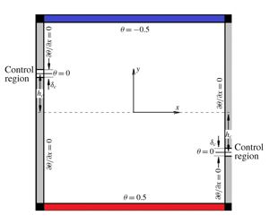
 $$\begin{eqnarray}\left.\begin{array}{@{}c@{}}\unicode[STIX]{x1D735}\boldsymbol{\cdot }\boldsymbol{u}=0,\\ \unicode[STIX]{x2202}\boldsymbol{u}/\unicode[STIX]{x2202}t+\boldsymbol{u}\boldsymbol{\cdot }\unicode[STIX]{x1D735}\boldsymbol{u}=-\unicode[STIX]{x1D735}p+(Ra/Pr)^{-1/2}\unicode[STIX]{x1D6FB}^{2}\boldsymbol{u}+\unicode[STIX]{x1D703}\boldsymbol{j},\\ \unicode[STIX]{x2202}\unicode[STIX]{x1D703}/\unicode[STIX]{x2202}t+\boldsymbol{u}\boldsymbol{\cdot }\unicode[STIX]{x1D735}\unicode[STIX]{x1D703}=(Ra\,Pr)^{-1/2}\unicode[STIX]{x1D6FB}^{2}\unicode[STIX]{x1D703},\\ y=-0.5:\quad \boldsymbol{u}=0,\quad \unicode[STIX]{x1D703}=0.5,\\ y=0.5:\quad \boldsymbol{u}=0,\quad \unicode[STIX]{x1D703}=-0.5,\\ x=-0.5:\quad \boldsymbol{u}=0,\quad \unicode[STIX]{x1D6FC}_{l}\unicode[STIX]{x1D703}+(1-\unicode[STIX]{x1D6FC}_{l})\unicode[STIX]{x2202}\unicode[STIX]{x1D703}/\unicode[STIX]{x2202}x=0,\\ x=0.5:\quad \boldsymbol{u}=0,\quad \unicode[STIX]{x1D6FC}_{r}\unicode[STIX]{x1D703}+(1-\unicode[STIX]{x1D6FC}_{r})\unicode[STIX]{x2202}\unicode[STIX]{x1D703}/\unicode[STIX]{x2202}x=0,\end{array}\right\}\end{eqnarray}$$
 where Rayleigh number  $Ra={\hat{g}}\hat{\unicode[STIX]{x1D6FD}}\unicode[STIX]{x0394}\hat{\unicode[STIX]{x1D703}}{\hat{H}}^{3}/(\hat{\unicode[STIX]{x1D708}}\hat{\unicode[STIX]{x1D6FC}})$, Prandtl number
  $Pr=\hat{\unicode[STIX]{x1D708}}/\hat{\unicode[STIX]{x1D6FC}}$ and the coefficients governing the temperature boundary conditions on the sidewalls are
 $$\begin{eqnarray}\unicode[STIX]{x1D6FC}_{l}=\left\{\begin{array}{@{}ll@{}}0,\quad & |y-h_{c}|\geqslant \unicode[STIX]{x1D6FF}_{c}/2,\\ 1,\quad & |y-h_{c}|<\unicode[STIX]{x1D6FF}_{c}/2,\end{array}\right.\quad \text{and}\quad \unicode[STIX]{x1D6FC}_{r}=\left\{\begin{array}{@{}ll@{}}0,\quad & |y+h_{c}|\geqslant \unicode[STIX]{x1D6FF}_{c}/2,\\ 1,\quad & |y+h_{c}|<\unicode[STIX]{x1D6FF}_{c}/2.\end{array}\right.\end{eqnarray}$$
 This means that the sidewalls are adiabatic except for two  $\unicode[STIX]{x1D703}=0$ regions with the same width
  $\unicode[STIX]{x1D6FF}_{c}$ around
  $y=h_{c}$ on the left wall and around
  $y=-h_{c}$ on the right wall. For simplicity, we will only mention about the control on the right wall with
  $h_{c}\geqslant 0$ in the following discussions. Similar boundary conditions can be seen in Tangborn (Reference Tangborn1992) and Ripesi et al. (Reference Ripesi, Biferale, Sbragaglia and Wirth2014). A sketch of the flow set-ups and the related boundary conditions are shown in figure 1.
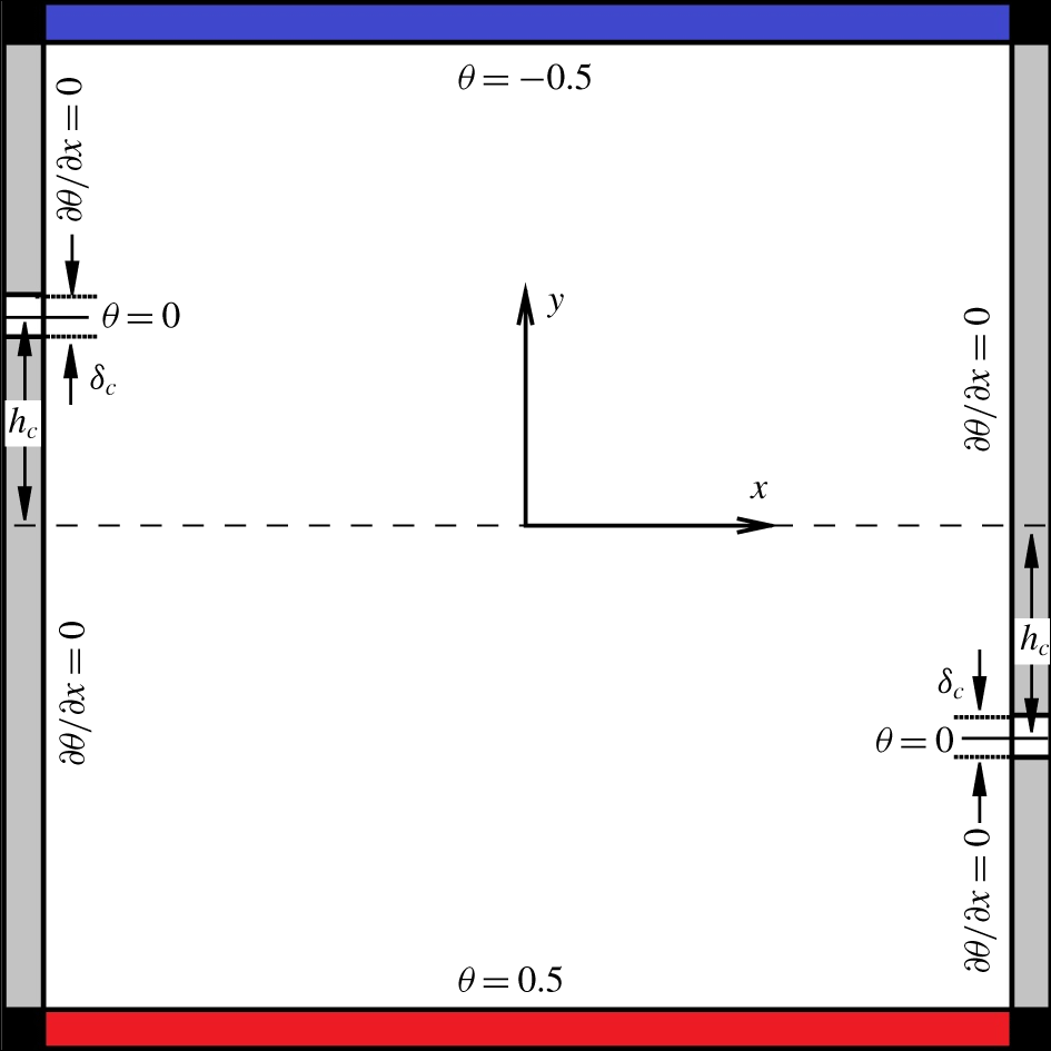
Figure 1. Sketch of sidewall-controlled RBC with  $h_{c}>0$.
2.2 Simulation parameters
In the present work, the above equation (2.1) are solved using the second-order central difference code developed by Zhang & Bao (Reference Zhang and Bao2015). Three groups of simulations were carried out. The first group is at  $Ra=5\times 10^{7}$ and
  $Pr=2$, where the flow reversal happens for adiabatic sidewalls, with varying
  $h_{c}$ and
  $\unicode[STIX]{x1D6FF}_{c}$ in order to obtain a phase diagram where the control can successfully eliminate the reversal. The value of
  $h_{c}$ varies in
  $[0,0.45]$ with interval 0.05, while
  $\unicode[STIX]{x1D6FF}_{c}$ varies in
  $[0,0.1]$ with interval 0.01, resulting in 101 simulations. The second group is at
  $Ra=5\times 10^{7}$ and
  $Pr=6$ with
  $h_{c}=0$, where no reversal occurs for adiabatic sidewalls in order to show the possibility of activating the reversal. The third group is at
  $Ra=1\times 10^{8}$ and
  $Pr=2$ with certain
  $h_{c}$ and
  $\unicode[STIX]{x1D6FF}_{c}$ to show the Rayleigh-number effect of the control.
The number of grid points is  $384\times 384$ for
  $Ra=5\times 10^{7}$ and
  $1152\times 1152$ for
  $Ra=1\times 10^{8}$, and the corresponding time intervals are
  $1.0\times 10^{-3}$ and
  $2.0\times 10^{-4}$. The grid size
  $\unicode[STIX]{x1D6E5}$ satisfies
  $\unicode[STIX]{x1D6E5}<0.37\min [\unicode[STIX]{x1D702}_{K},\unicode[STIX]{x1D702}_{B}]$ where
  $\unicode[STIX]{x1D702}_{K}=(\hat{\unicode[STIX]{x1D708}}^{3}/\hat{\unicode[STIX]{x1D700}}(\boldsymbol{x},t))^{1/4}/{\hat{H}}$ (with
  $\hat{\unicode[STIX]{x1D700}}(\boldsymbol{x},t)$ being the local turbulent dissipation) and
  $\unicode[STIX]{x1D702}_{B}=\unicode[STIX]{x1D702}_{K}Pr^{-1/2}$ are the local Kolmogorov scale and Batchelor scale, respectively, which can be estimated by scaling laws in the boundary layer as suggested by Shishkina et al. (Reference Shishkina, Stevens, Grossmann and Lohse2010). The time step is small enough so that the Courant–Friedrichs–Lewy number is smaller than 0.2.
In the following,  $\langle \cdot \rangle _{t}$,
  $\langle \cdot \rangle _{x}$ and
  $\langle \cdot \rangle _{y}$ denote the average in time, along the
  $x$ axis and along the
  $y$ axis, respectively. The averaged vortex turnover time
  $t_{E}$ is
  $t_{E}=4\unicode[STIX]{x03C0}/\langle |\unicode[STIX]{x1D714}(0,0,t)|\rangle _{t}$ where
  $\unicode[STIX]{x1D714}(0,0,t)$ is the central vorticity (Sugiyama et al. Reference Sugiyama, Ni, Stevens, Chan, Zhou, Xi, Sun, Grossmann, Xia and Lohse2010). In order to check the existence of reversals, simulations are performed for more than
  $1000t_{E}$ for all cases. However, due to the stochastic feature of turbulence, the absence of reversals cannot be confirmed with finite simulation time. Therefore, in the present context, ‘no reversal’ means no reversal observed in
  $1000t_{E}$. Nevertheless, considering the traditional mean time intervals
  ${\sim}30t_{E}$ in the present
  $Ra$ range (Sugiyama et al. Reference Sugiyama, Ni, Stevens, Chan, Zhou, Xi, Sun, Grossmann, Xia and Lohse2010),
  $1000t_{E}$ can be viewed as a reasonably long time period. For accuracy of the flow statistics, the simulations were run for
  $5000t_{E}$ and the statistics are computed within a time range over
  $4000t_{E}$.
3 Simulation results and discussion
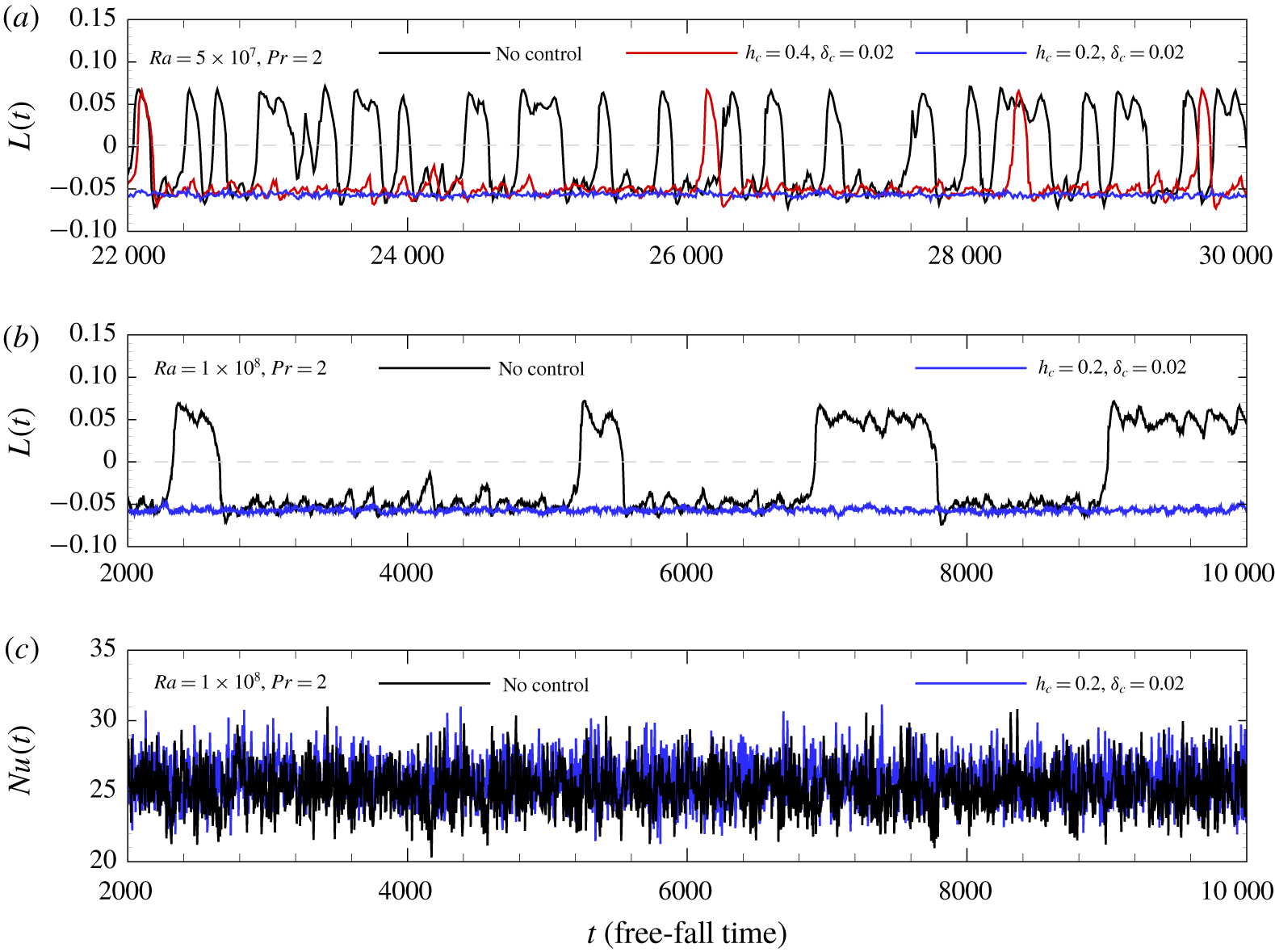
Figure 2. (a,b) Time series of (a)  $L(t)$ at
  $Ra=5\times 10^{7}$ and
  $Pr=2$, no control with adiabatic sidewalls (black),
  $h_{c}=0.4,\unicode[STIX]{x1D6FF}_{c}=0.02$ (red) and
  $h_{c}=0.2,\unicode[STIX]{x1D6FF}_{c}=0.02$ (blue); and (b)
  $L(t)$ at
  $Ra=1\times 10^{8}$ and
  $Pr=2$, no control with adiabatic sidewalls (black) and
  $h_{c}=0.2,\unicode[STIX]{x1D6FF}_{c}=0.02$ (blue). Values
  $L>0$ indicates anticlockwise circulation, while
  $L<0$ indicates clockwise circulation. (c) Plot of
  $Nu(t)$ at
  $Ra=1\times 10^{8}$ and
  $Pr=2$ with the same colouring rule as in panel (b).
Flow reversal can be identified through different approaches, such as the temperature contrast between the left and right walls (Chen et al. Reference Chen, Huang, Xia and Xi2019) and the sign change of angular momentum (Sugiyama et al. Reference Sugiyama, Ni, Stevens, Chan, Zhou, Xi, Sun, Grossmann, Xia and Lohse2010; Wang et al. Reference Wang, Xia, Wang, Sun, Zhou and Wan2018). Here, we are using the latter, and the angular momentum is defined as (Sugiyama et al. Reference Sugiyama, Ni, Stevens, Chan, Zhou, Xi, Sun, Grossmann, Xia and Lohse2010)
 $$\begin{eqnarray}L(t)=\langle x\cdot v-y\cdot u\rangle _{x,y}.\end{eqnarray}$$
 Figure 2(a) shows the time series of the angular momentum  $L(t)$ at
  $Ra=5\times 10^{7}$ and
  $Pr=2$ in a time period of 8000 free-fall times. Three cases were considered, including no control with adiabatic sidewalls, and constant sidewall control with
  $h_{c}=0.4,\unicode[STIX]{x1D6FF}_{c}=0.02$ and with
  $h_{c}=0.2,\unicode[STIX]{x1D6FF}_{c}=0.02$. In the situation of no control,
  $L(t)$ changes its sign frequently, 43 times, in the time period shown, resulting in a mean time interval
  $\langle \unicode[STIX]{x1D70F}\rangle \approx 28.2t_{E}$ between successive reversals (
 $t_{E}\approx 6.6$ free-fall times). When sidewall control with a small width
  $\unicode[STIX]{x1D6FF}_{c}=0.02$ is applied near the right bottom corner, i.e.
  $h_{c}=0.4$, the flow reversal still happens but its frequency reduces a lot. When the control region moves towards the centre height to
  $h_{c}=0.2$, one has
  $L(t)<0$ in the whole time period, indicating a successful elimination of the flow reversal.
From these results, we may say that the sidewall control will affect the occurrence of the flow reversal, and it can successfully eliminate the flow reversal if  $h_{c}$ and
  $\unicode[STIX]{x1D6FF}_{c}$ are chosen properly. This is also true when
  $Ra$ increases to
  $Ra=1\times 10^{8}$, as shown in figure 2(b), where the time series of
  $L(t)$ with or without sidewall control are shown. Again, the flow reversal, which happens without sidewall control, can be eliminated successfully with sidewall control with
  $h_{c}=0.2,\unicode[STIX]{x1D6FF}_{c}=0.02$.
Figure 2(c) shows the time series of the instantaneous Nusselt number in the vertical direction, which is defined as
 $$\begin{eqnarray}Nu(t)=-\frac{1}{2}\left[\left.\frac{\unicode[STIX]{x2202}\langle \unicode[STIX]{x1D703}\rangle _{x}}{\unicode[STIX]{x2202}y}\right|_{y=-0.5}+\left.\frac{\unicode[STIX]{x2202}\langle \unicode[STIX]{x1D703}\rangle _{x}}{\unicode[STIX]{x2202}y}\right|_{y=0.5}\right],\end{eqnarray}$$
 in the same two cases as in figure 2(b). It is seen that  $Nu(t)$ in both cases oscillates severely, while the controlled case with
  $h_{c}=0.2,\unicode[STIX]{x1D6FF}_{c}=0.02$ has a slightly larger mean value. Compared to the no-control case, where the time-averaged Nusselt number in the vertical direction is
  $\langle Nu\rangle _{t}=25.19$, in the controlled case
  $\langle Nu\rangle _{t}$ increases by approximately 2.2 % and reaches
  $25.74$. This means that the slight sidewall control not only can suppress the flow reversal, but also can enhance the heat transfer in the vertical direction.
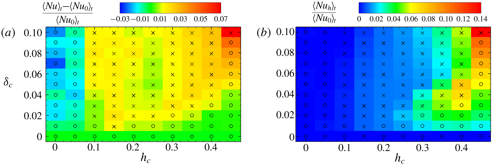
Figure 3. Phase diagram in the  $h_{c}{-}\unicode[STIX]{x1D6FF}_{c}$ plane with contours of relative values of Nusselt numbers for
  $Ra=5\times 10^{7}$ and
  $Pr=2$. Crosses correspond to no detected reversals and circles to detected reversals.
  $Nu_{0}$ denotes the vertical Nusselt number of the case without control. (a) Relative value of time-averaged vertical Nusselt number
  $\langle Nu\rangle _{t}$. (b) Relative value of time-averaged horizontal Nusselt number
  $\langle Nu_{h}\rangle _{t}$.
Figure 3 shows the phase diagram of occurrence of reversals for fixed physical parameters  $Ra=5\times 10^{7}$ and
  $Pr=2$ and varying control parameters
  $h_{c}$ and
  $\unicode[STIX]{x1D6FF}_{c}$, together with the relative value of the time-averaged Nusselt number in the vertical direction
  $\langle Nu\rangle _{t}$ (figure 3a) and in the horizontal direction
  $\langle Nu_{h}\rangle _{t}$ (figure 3b) compared to the no-control case at the same
  $Ra$ and
  $Pr$. Here, the Nusselt number in the horizontal direction
  $Nu_{h}$ is defined similarly as
 $$\begin{eqnarray}Nu_{h}=-\frac{1}{2}\left[\left.\frac{\unicode[STIX]{x2202}\langle \unicode[STIX]{x1D703}\rangle _{y}}{\unicode[STIX]{x2202}x}\right|_{x=-0.5}+\left.\frac{\unicode[STIX]{x2202}\langle \unicode[STIX]{x1D703}\rangle _{y}}{\unicode[STIX]{x2202}x}\right|_{x=0.5}\right].\end{eqnarray}$$
 It is seen again that the sidewall control with constant temperature can eliminate the flow reversal if  $h_{c}$ and
  $\unicode[STIX]{x1D6FF}_{c}$ are chosen in proper ranges. When
  $h_{c}\leqslant 0.05$, the reversal always happens even when
  $\unicode[STIX]{x1D6FF}_{c}$ is as large as 0.1, which means that the control location should not be placed near the sidewall centre. On the other hand, if the control zone is placed near the right bottom corner, that is
  $h_{c}=0.45$, it is also very hard to eliminate the reversal and a successful elimination of flow reversal happens only when a very wide control region
  $\unicode[STIX]{x1D6FF}_{c}=0.1$ is applied, i.e.
  $\unicode[STIX]{x1D703}=0$ is near the right bottom corner
  $-0.5<y<-0.4$. In the range
  $0.10\leqslant h_{c}\leqslant 0.40$, the control is very effective, and the flow reversal can be prevented if
  $\unicode[STIX]{x1D6FF}_{c}\geqslant 0.04$. The
  $\unicode[STIX]{x1D6FF}_{c}$ value can be further reduced when the control location
  $h_{c}$ moves to its optimal position
  $h_{c}\approx 0.15$, where a very small width
  $\unicode[STIX]{x1D6FF}_{c}=0.01$ can effectively eliminate the reversal.
The contour in figure 3(a) shows that there is an increase of  $\langle Nu\rangle _{t}$ for the controlled cases when
  $h_{c}\geqslant 0.1$ while it will decrease if
  $h_{c}\leqslant 0.05$. This is probably because the sidewall control with
  $h_{c}\geqslant 0.1$ could stabilize large-scale structures and suppress flow reversals, which in turn would enhance the heat transfer in the vertical direction up to a few per cent, while the sidewall control with
  $h_{c}\leqslant 0.05$ could enhance the flow reversal and reduce the heat transfer in the vertical direction. The increase is generally below 5 %, except for the
  $h_{c}=0.45,\unicode[STIX]{x1D6FF}_{c}=0.1$ case, where the variation is approximately 7 %, while the reduction could be approximately 3 %. Both increase and decrease of
  $\langle Nu\rangle _{t}$ seem to be non-monotonic for
  $h_{c}$ or
  $\unicode[STIX]{x1D6FF}_{c}$.
For the horizontal heat transfer, as shown by the contours in figure 3(b), it is seen that  $\langle Nu_{h}\rangle _{t}$ increases generally with
  $h_{c}$. We attribute this phenomenon to the fact that with
  $h_{c}$ increasing there is an increase of heat transfer between the sidewalls and horizontal plates through hot/cold plumes and direct thermal conduction. Interestingly,
  $\langle Nu_{h}\rangle _{t}$ varies in a much wider range as compared to
  $\langle Nu\rangle _{t}$, and the largest increase could be as much as
  $0.14\langle Nu_{0}\rangle _{t}$. Again,
  $\langle Nu_{h}\rangle _{t}$ seems to be non-monotonic for
  $\unicode[STIX]{x1D6FF}_{c}$ at
  $h_{c}\leqslant 0.4$. The non-monotonic behaviours in both
  $\langle Nu\rangle _{t}$ and
  $\langle Nu_{h}\rangle _{t}$ may illustrate the complex coupling between the vertical and horizontal heat transfer under the sidewall control.
Sugiyama et al. (Reference Sugiyama, Ni, Stevens, Chan, Zhou, Xi, Sun, Grossmann, Xia and Lohse2010) described the role of the corner flows during the reversal process. Owing to energetic feeding by the detaching plumes from the boundary layers trapped in the corner, the small corner rolls will grow until they reach the half-height, and then they will destroy the main LSC and establish another LSC in the opposite direction. Nevertheless, the reversals are not in perfect periodicity (see figure 2) and sometimes the corner rolls remain oscillating around a certain size (the height of the corner roll  $h$ oscillates by approximately 0.38; see the supplementary movie 1 and figure 2(a) of Sugiyama et al. (Reference Sugiyama, Ni, Stevens, Chan, Zhou, Xi, Sun, Grossmann, Xia and Lohse2010) available at https://doi.org/10.1017/jfm.2020.210). Without loss of generality, we will focus on the right side of the flow in a clockwise LSC state in the following discussions.
Part of the detached hot plumes will rise up along the right sidewall due to the right corner roll, and then they will encounter and interact with the cold plumes carried by the main LSC. The interaction makes the hot plumes separate from the sidewall and descend back towards the bottom plate. The sidewall control below the separation point of the hot plume on the sidewall can absorb the heat from the hot plume and lower its temperature, and thus reduce the corner roll’s kinetic energy input provided by the work of the buoyancy force, breaking the feeding process of the corner rolls. This results in the locking of the corner rolls into a smaller region near the corner, making it harder for a reversal to occur. However, when the control region moves close to the bottom plate, the efficiency of reversal suppression is even lower, although the heat absorbed by the sidewall increases, as shown in figure 3(b). Furthermore, the reduction of the corner roll’s energy feeding argument cannot explain the fact that the best control region is approximately  $h_{c}=0.15$ for the present
  $Ra$ and
  $Pr$. Therefore, we infer that the reduction of the corner roll’s energy feeding is not the only mechanism for the reversal suppression with sidewall control.
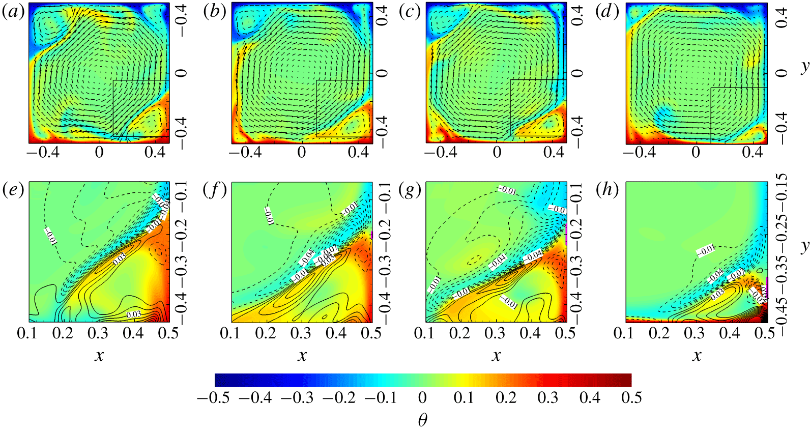
Figure 4. Temperature contours, velocity vectors and contours of  $F_{x}^{b}$ (levels
  $-0.1(0.01)0.1$) of instantaneous fields at
  $Ra=5\times 10^{7}$ and
  $Pr=2$ with different
  $h_{c}$ and
  $\unicode[STIX]{x1D6FF}_{c}$: (a,e) no control,
  $t=10\,422$; (b,f)
  $h_{c}=0.2,\unicode[STIX]{x1D6FF}_{c}=0.02,t=10\,027$; (c,g)
  $h_{c}=0.2,\unicode[STIX]{x1D6FF}_{c}=0.06,t=10\,075$; and (d,h)
  $h_{c}=0.4,\unicode[STIX]{x1D6FF}_{c}=0.06,t=10\,466$. (a–d) Temperature and velocity vectors; (e–h) temperature and
  $F_{x}^{b}$. Also see the supplementary movies 1, 2, 3 and 4, respectively.
Considering the situation when the hot plumes flow past the control region, the  $\unicode[STIX]{x1D703}=0$ wall would cool down the neighbouring fluid and create a small
  $\unicode[STIX]{x1D703}\approx 0$ region (see figure 4f–h). Owing to the temperature difference, the
  $\unicode[STIX]{x1D703}\approx 0$ fluid tends to descend relative to the surrounding hot fluid and behaves like an obstacle that forces the hot plume to separate from the sidewall in order to bypass it. Such a mechanism originates from the local variation of buoyancy force and can be quantitatively evaluated using the divergence-free buoyancy force
  $\boldsymbol{F}^{b}=\unicode[STIX]{x1D703}\boldsymbol{j}-\unicode[STIX]{x1D735}p_{\unicode[STIX]{x1D703}}$. Here,
  $p_{\unicode[STIX]{x1D703}}$ is the buoyancy-induced pressure and its governing equation is
 $$\begin{eqnarray}\unicode[STIX]{x1D6FB}^{2}p_{\unicode[STIX]{x1D703}}=\unicode[STIX]{x2202}\unicode[STIX]{x1D703}/\unicode[STIX]{x2202}y,\quad \unicode[STIX]{x2202}p_{\unicode[STIX]{x1D703}}/\unicode[STIX]{x2202}x|_{x=\pm 0.5}=0,\quad \unicode[STIX]{x2202}p_{\unicode[STIX]{x1D703}}/\unicode[STIX]{x2202}y|_{y=\pm 0.5}=\unicode[STIX]{x1D703}.\end{eqnarray}$$
 Above,  $\boldsymbol{F}^{b}$ is the divergence-free projection of the buoyancy force and it corresponds to the net contribution of the temperature field to the velocity fields.
Figure 4 shows the instantaneous velocity vectors, contours of temperature and the horizontal component of the divergence-free buoyancy force  $F_{x}^{b}$ at
  $Ra=5\times 10^{7}$ and
  $Pr=2$ without sidewall control (not during the reversal event) and with different sidewall controls. Figure 4(b–d) indicates that the separation of the hot plume happens near the control region for controlled cases. The supplementary movies 1–4 also show that the separation points are relatively stable for the three controlled cases. Negative
  $F_{x}^{b}$ with relatively larger magnitude close to the wall is found near the separation point of the hot plume just below the control region as shown in figure 4(f–h) and the supplementary movies 2–4. Since the local influence of temperature on the velocity field only exists in the projected buoyancy force, it is straightforward to claim that the increase of near-wall
  $F_{x}^{b}$ pointing inwards should be the main reason for plumes to separate near the control region, and we believe that this direct forcing of the plume to separate from the sidewall near the control region could be the second mechanism of reversal suppression.
In fact, the sidewall control not only can suppress/eliminate the flow reversal, but also can activate/enhance the flow reversal. Figure 5 shows the time series of angular momentum  $L(t)$ from different simulations at
  $Ra=5\times 10^{7}$ and
  $h_{c}=0$. In figure 5(a), we study the cases at
  $Pr=6$. At
  $Pr=6$ and
  $Ra=5\times 10^{7}$, there is no flow reversal without sidewall control (Sugiyama et al. Reference Sugiyama, Ni, Stevens, Chan, Zhou, Xi, Sun, Grossmann, Xia and Lohse2010) and
  $L(t)$ will not change its sign as time evolves, as depicted by the black lines. However, if the sidewall control is applied at the sidewall centre, i.e.
  $h_{c}=0$, the flow reversal may happen. With a small width
  $\unicode[STIX]{x1D6FF}_{c}=0.02$ (red lines), the reversal does occur, and
  $L(t)$ changes its sign four times during 5000 free-fall times. More importantly, there seem to be two different flow states, as displayed by the insets at two different time steps. At one state, there is one main LSC, clockwise or anticlockwise (single-roll mode, right inset). At the other state, there are two counter-rotating rolls aligned in the vertical directions (double-roll mode, left inset). Multiple states with single-roll mode and double-roll mode have been reported before by Xi & Xia (Reference Xi and Xia2008) in cylindrical RBC at higher
  $Ra$. In their experimental work, the averaged percentages of time that the large-scale mean flow spends in double-roll mode is only 0.8 %. Here, with the sidewall control, we could enhance the appearance of the double-roll mode. With a much wider width
  $\unicode[STIX]{x1D6FF}_{c}=0.06$ (blue lines), it is seen that the flow reversal happens more frequently, and
  $L(t)$ changes its sign 28 times in the same 5000 free-fall times. Furthermore, from the oscillating amplitudes of
  $L(t)$, it is easy to infer that the flow will experience multiple states as the controlled case with
  $\unicode[STIX]{x1D6FF}_{c}=0.02$ (see the supplementary movie 5), and the appearance probability of the double-roll mode is also higher.
At  $Pr=2$ and
  $Ra=5\times 10^{7}$, where the flow will experience flow reversals without sidewall control, the sidewall control with a small width
  $\unicode[STIX]{x1D6FF}_{c}=0.02$ can still enhance the reversal events, as displayed in figure 5(b). It is apparent that
  $L(t)$ changes its sign more frequently, and it might oscillate with a lower amplitude (see the time period
  $28\,000<t<29\,000$), inferring a second flow state in double-roll mode of the large-scale motions. The activation/enhancement of the flow reversals with control near the sidewall centre (
 $h_{c}\approx 0$) can also be explained using the two mechanisms discussed above. Differently from the suppression/elimination cases, the control region with
  $h_{c}\approx 0$ will break the feeding process of the main LSC instead of the corner rolls, smashing in the balance between the LSC and corner rolls and making the flow reversal easier to occur. Furthermore, the control region also makes the plumes separate from the sidewall, and this in turn can determine the size of the LSC and corner rolls.
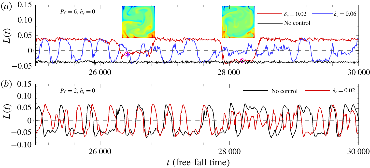
Figure 5. Time series of angular momentum  $L(t)$ from different simulations at
  $Ra=5\times 10^{7}$ and
  $h_{c}=0$: (a)
  $Pr=6$ with no control (black lines),
  $\unicode[STIX]{x1D6FF}_{c}=0.02$ (red lines) and
  $\unicode[STIX]{x1D6FF}_{c}=0.06$ (blue lines); and (b)
  $Pr=2$ with no control (black lines) and
  $\unicode[STIX]{x1D6FF}_{c}=0.02$ (red lines). The two insets in (a) represent the instant temperature contours from the simulation with
  $\unicode[STIX]{x1D6FF}_{c}=0.02$ at
  $t=26\,400$ and
  $t=28\,200$, respectively.
Finally, it is also very intuitive to explain the reversal suppression/enhancement using the concept of symmetry:  $h_{c}>H_{c}$ (
 $H_{c}$ is the bound that separates the suppression/enhancement of the sidewall control, and it is around 0.05 at
  $Pr=2$ and
  $Ra=5\times 10^{7}$) breaks the symmetry about lines
  $x=0$ and
  $y=0$ and favours a clockwise state, while
  $h_{c}=0$ strengthens the symmetry of the system, motivating LSC to reverse more frequently and even inducing a double-roll mode consequently.
4 Conclusion
In traditional RBC, the sidewalls are adiabatic, and the LSC reversals may happen in a certain range of  $Ra$ and
  $Pr$. In this paper, we reported through a series of direct numerical simulations in 2-D RBC that the LSC reversals can be suppressed or enhanced when a local
  $\unicode[STIX]{x1D703}=0$ control is applied on the sidewalls. When the control region is located near the centre region (
 $0\leqslant h_{c}\leqslant H_{c}$), the flow reversal can be enhanced or even activated if there is no reversal without controls. The sidewall control at the centre (
 $h_{c}=0$) can also stimulate the occurrence of the double-roll mode. When the sidewall control is located away from the centre region (
 $h_{c}>H_{c}$), the flow reversal will be suppressed while convective heat transfer in the vertical direction will be enhanced. As
  $\unicode[STIX]{x1D6FF}_{c}$ increases, the probability of occurrence of the reversal becomes lower and it can be successfully eliminated if
  $\unicode[STIX]{x1D6FF}_{c}$ is large enough. For
  $h_{c}=0.15$, flow reversals could be stopped with a control area less than
  $0.01$. The specific mechanism of reversal control is that control regions could weaken plumes through heat conduction and they could also force the plumes to separate from the sidewalls. Besides, the concept of symmetry is also helpful in the interpretation of control mechanisms.
The results of the present work are quite elementary, but it opens a new idea to the community to control the flow reversal through modifying the sidewall boundary conditions. The results of the present work have extensive potential applications in industry, geophysics and astrophysics, especially in the circumstances where only small and local changes could be applied to the boundaries. In the future, we will test the effectiveness of the control strategy in quasi-2-D and fully 3-D RBC through both numerical simulations and experiments.
Acknowledgements
This work was supported by the National Science Foundation of China (NSFC grant nos 11822208, 11772297, 91852205 and 11825204). The numerical simulations were finished at the National Supercomputer Center in Guangzhou (Tianhe-2A), China.
Declaration of interests
The authors report no conflict of interest.
Supplementary movies
Supplementary movies are available at https://doi.org/10.1017/jfm.2020.210.


