


1 Introduction
Ostwald ripening is a phase coarsening phenomenon that has been observed in various systems where a dispersed second phase is present (Greenwood Reference Greenwood1956; Lifshitz & Slyozov Reference Lifshitz and Slyozov1961; Plesset & Sadhal Reference Plesset and Sadhal1982; Voorhees Reference Voorhees1985, Reference Voorhees1992). In a bulk liquid, the dispersed phase in the form of bubbles is coarsened by growth of large bubbles at the expense of small bubbles. Capillary pressure of a bubble can be expressed as a function of its radius according to Laplace’s law, i.e.
 $$\begin{eqnarray}P_{c}={\displaystyle \frac{2\unicode[STIX]{x1D70E}}{r}},\end{eqnarray}$$
 where  $P_{c}$ is the pressure difference between the two phases,
  $\unicode[STIX]{x1D70E}$ is the interfacial tension and
  $r$ is the interfacial radius. Coexistence of bubbles of different sizes leads to capillary pressure gradients within the system, serving as the driving force for Ostwald ripening. The mass fraction of dissolved gas species in the continuous phase adjacent to an interface is proportional to local capillary pressure according to Henry’s law, i.e.
 $$\begin{eqnarray}X={\displaystyle \frac{P_{w}+P_{c}}{H}},\end{eqnarray}$$
 where  $X$ is the mass fraction of dissolved gas species in the adjacent continuous phase,
  $P_{w}$ is the pressure of the continuous phase and
  $H$ is Henry’s constant. This mass fraction gradient drives mass flux from the bubbles with high capillary pressure toward regions of low capillary pressure.
In a bulk liquid, the interfacial radius is equivalent to the bubble radius because the interface is spherical and can grow without spatial restriction. In a porous medium, however, the presence of a solid matrix adds complexity to the Ostwald ripening process. The shape of each individual ganglion is strongly restricted by local pore topography, and interfacial radii at free interfaces are strongly dependent on pore geometry (Bear Reference Bear2013). Given the circumstances, capillary pressure of a ganglion is rather a complex function of local pore topography and pore size instead of its volume (Garing et al. Reference Garing, de Chalendar, Voltolini, Ajo-Franklin and Benson2017). This fact leads to difficulty when predicting mass redistribution of dispersed ganglia by Ostwald ripening due to capillary pressure gradients.
Past studies of Ostwald ripening in porous media have dealt with this complexity in a number of ways. For example, Ostwald ripening has been neglected because concentration gradients imposed by the rate of change of the supersaturation were significantly larger than those driving Ostwald ripening (Li & Yortsos Reference Li and Yortsos1995; Tsimpanogiannis & Yortsos Reference Tsimpanogiannis and Yortsos2002). Other studies on Ostwald ripening in porous media neglected capillary pressure gradients (Dominguez, Bories & Prat Reference Dominguez, Bories and Prat2000; Goldobin & Brilliantov Reference Goldobin and Brilliantov2011). In recent years, Ostwald ripening in porous media driven by capillary pressure gradients has gained researchers’ attention due to its potential application to geological carbon sequestration (Garing et al. Reference Garing, de Chalendar, Voltolini, Ajo-Franklin and Benson2017; Xu, Bonnecaze & Balhoff Reference Xu, Bonnecaze and Balhoff2017; de Chalendar, Garing & Benson Reference de Chalendar, Garing and Benson2018). In particular, one important mechanism of immobilizing  $\text{CO}_{2}$ is referred to as residual trapping, where injected
  $\text{CO}_{2}$ is residually trapped in the form of disconnected ganglia by capillary forces (Hesse, Orr & Tchelepi Reference Hesse, Orr and Tchelepi2008; Bear Reference Bear2013). If residual
  $\text{CO}_{2}$ ganglia coexist at different capillary pressures, the resulting capillary pressure gradients will initiate Ostwald ripening. Consequently, ganglia may shrink or grow resulting in redistribution of residual
  $\text{CO}_{2}$ and potentially, re-aggregation of initially disconnected
  $\text{CO}_{2}$.
To evaluate the potential for Ostwald ripening in porous media, it is necessary to determine the capillary pressure of a single ganglion. Andrew, Bijeljic & Blunt (Reference Andrew, Bijeljic and Blunt2014) imaged trapped  $\text{CO}_{2}$ ganglia in a limestone sample at reservoir conditions and calculated curvatures of
  $\text{CO}_{2}$–brine interfaces. The measured curvatures over a single ganglion display a well-defined peak, indicating that a single ganglion is present at a single value of capillary pressure. This observation is also supported by an analysis on interfacial curvatures in an air–brine system performed by Garing et al. (Reference Garing, de Chalendar, Voltolini, Ajo-Franklin and Benson2017).
In addition to a single ganglion, studies have shown that a group of adjacent ganglia can reach local capillary equilibrium. de Chalendar et al. (Reference de Chalendar, Garing and Benson2018) developed a pore-network model for simulating Ostwald ripening accounting for capillary effects using conically-shaped pore throats. The authors demonstrated that  $\text{CO}_{2}$ ganglia across several pores with initially different capillary pressures could eventually approach capillary equilibrium by inter-ganglion diffusion on the time scale of years. This finding was supported by a two-and-a-half-dimensional micro-model experiment (Xu et al. Reference Xu, Bonnecaze and Balhoff2017), where the authors reported that trapped gas ganglia with initially different sizes can eventually approach a uniform size. Furthermore, Garing et al. (Reference Garing, de Chalendar, Voltolini, Ajo-Franklin and Benson2017) showed that the equilibrium capillary pressure of trapped air ganglia is roughly at the same order of the entry pressure of the porous medium. This observation implied that not only is there a potential for Ostwald ripening among local ganglia across several pores, but also among the groups of ganglia in porous media with different entry pressures.
The above findings of Garing et al. (Reference Garing, de Chalendar, Voltolini, Ajo-Franklin and Benson2017) and de Chalendar et al. (Reference de Chalendar, Garing and Benson2018) give rise to a new scenario of Ostwald ripening in the context of geological  $\text{CO}_{2}$ sequestration. Supercritical
  $\text{CO}_{2}$ is injected into a reservoir and forms a
  $\text{CO}_{2}$ plume that flows laterally and upward driven by viscous and buoyancy forces. After injection stops, reservoir water imbibes into the
  $\text{CO}_{2}$ plume and traps
  $\text{CO}_{2}$ in the form of residual
  $\text{CO}_{2}$. Residually trapped
  $\text{CO}_{2}$ could reach local capillary equilibrium rapidly at the same order of the local entry pressure. Capillary heterogeneity can be observed at various spatial scales above the representative elementary volume (REV) such as from the sub-core scale to the reservoir scale and results in variation of local entry pressure (Van Genuchten Reference Van Genuchten1980; Pini, Krevor & Benson Reference Pini, Krevor and Benson2012). Therefore, different sections of a heterogeneous reservoir have different capillary pressure curves. These capillary pressure gradients can initiate Ostwald ripening among locally equilibrated residually trapped
  $\text{CO}_{2}$ and may result in
  $\text{CO}_{2}$ redistribution in the reservoir even though the
  $\text{CO}_{2}$ ganglia are completely trapped. Therefore, it is crucial to evaluate the impact of Ostwald ripening in this scenario on residual
  $\text{CO}_{2}$ and evaluate the time scale for redistribution, owing to the fact that redistribution may re-aggregate disconnected
  $\text{CO}_{2}$ and remobilize the trapped
  $\text{CO}_{2}$.

Figure 1. A continuum-scale conceptual representation of Ostwald ripening of residually trapped  $\text{CO}_{2}$. (a) An illustration of the initial condition. The
  $\text{CO}_{2}$ ganglia are trapped in pore spaces and at local capillary equilibrium. Their interfacial curvatures are uniform within a domain and different between domains. (b) Capillary pressure distribution at the initial condition. The initial condition is at the end of imbibition where capillary pressures of residual
  $\text{CO}_{2}$ are represented by the endpoints of imbibition capillary pressure curves. (c) An illustration at equilibrium. Trapped
  $\text{CO}_{2}$ ganglia shrink or grow due to Ostwald ripening, and their interfacial curvatures approach the same value between domains. (d) Capillary pressure distribution at equilibrium. The
  $\text{CO}_{2}$ saturation within the two domains redistributes due to Ostwald ripening and approach capillary equilibrium between domains.
To this end, we investigate the consequences of Ostwald ripening on the equilibrium of residually trapped  $\text{CO}_{2}$ driven by reservoir heterogeneity. Three contributions are made in this paper. Firstly, we use a continuum-scale multi-physics numerical model to demonstrate redistribution of residually trapped
  $\text{CO}_{2}$ by Ostwald ripening. Secondly, we develop an analogous retardation factor based on the mathematical model of Ostwald ripening to compare the time scale of capillary equilibrium to that of single-phase diffusion. Lastly, we develop a new approximate solution for predicting the redistribution of residually trapped
  $\text{CO}_{2}$ over the entire course of evolution, serving as a tool to evaluate the importance of Ostwald ripening at various spatial scales and over a wide range of reservoir properties and initial conditions.
2 Continuum-scale numerical simulation of Ostwald ripening
2.1 The conceptual model
The conceptual model underlying this work is defined by re-equilibration between several adjacent domains of residual  $\text{CO}_{2}$ ganglia that are locally equilibrated within each domain, but are out of capillary equilibrium with the adjacent domains. During the re-equilibration period, residual
  $\text{CO}_{2}$ redistributes between the domains by diffusion of
  $\text{CO}_{2}$ through the aqueous phase, causing the capillary pressures of all domains to eventually approach the same value. When the spatial scale that ganglia groups expand over is above the REV, this pore-scale phenomenon manifests its effects at the continuum scale, where residual
  $\text{CO}_{2}$ saturation changes among domains. Here, we develop a continuum-scale model to link this redistribution to its pore-scale origins.
This model focuses on the supercritical  $\text{CO}_{2}$–water system, but could equally well be used for other pairs of immiscible fluids. The model is horizontal and one-dimensional with closed boundaries and consist of two domains. As shown in figure 1(a), the two domains are homogeneous respectively, while their capillary pressure curves are different as shown in figure 1(b). The two domains are connected to allow the aqueous phase to move freely between them so that the pressure in the aqueous phase is the same across the entire model.
The initial condition for this model is assumed to be shortly after imbibition, after pore-scale capillary equilibrium of the ganglia within each domain has been established, as shown in figure 1(b). The  $\text{CO}_{2}$ is assumed to be completely immobile with zero relative permeability at any saturation. The capillary pressure of the trapped
  $\text{CO}_{2}$ is assumed to be slightly above the entry pressure of the rock, as found in Garing et al. (Reference Garing, de Chalendar, Voltolini, Ajo-Franklin and Benson2017). The capillary pressure gradient between the two domains creates a
  $\text{CO}_{2}$ mass fraction gradient in the aqueous phase to drive
  $\text{CO}_{2}$ to diffuse from the high capillary pressure domain to the low capillary pressure domain. The saturation of
  $\text{CO}_{2}$ within the two domains redistributes during equilibration, and the two capillary pressures eventually approach equilibrium, as shown in figure 1(c,d).
We simply choose two imbibition capillary pressure curves to link residual  $\text{CO}_{2}$ saturation to capillary pressure for each domain. In the high capillary pressure domain, capillary pressure will decrease as it equilibrates with the other domain. We assume that this decrease in capillary pressure follows an extension of the imbibition curve, as shown in figure 1(d). The extension fulfils two requirements. Firstly, capillary pressure should decrease as
  $\text{CO}_{2}$ ganglia retreat from the pore throats towards the pore body. Secondly, the capillary pressure curve should not fall below the entry pressure of the rock. For the low capillary pressure domain, the capillary pressure will increase as Ostwald ripening occurs. We assume that during this period, the capillary pressure will follow the imbibition curves shown in figure 1(b). It should be noted that the imbibition capillary pressure curves chosen here only describe the mathematical relationship between residual
  $\text{CO}_{2}$ saturation and its capillary pressure instead of indicating the process to be imbibition. Conventionally, capillary pressure hysteresis only applies to the continuous non-wetting phase, and the residual non-wetting phase is excluded from the measurement of capillary pressure (Bear Reference Bear2013). Therefore, we do not adopt the concept of hysteresis to describe the capillary pressure change for residual
  $\text{CO}_{2}$ due to Ostwald ripening, and choosing imbibition curves is only for convenience as it represents a reasonable trend. The actual capillary pressure changes due to continuum-scale Ostwald ripening of residually trapped
  $\text{CO}_{2}$ could, in principle, be acquired by measuring the interfacial curvature through micro-CT imaging, although the long time scales would make this very challenging (Garing et al. Reference Garing, de Chalendar, Voltolini, Ajo-Franklin and Benson2017).
2.2 Description of the numerical model
The numerical simulator used for this problem is TOUGH2, a widely used simulator in problems relevant to flow in porous media such as geological  $\text{CO}_{2}$ sequestration and nuclear waste disposal (Pruess, Oldenburg & Moridis Reference Pruess, Oldenburg and Moridis1999). The equation-of-state ECO2N is adopted to describe the thermodynamic properties of
  $\text{CO}_{2}$–water–NaCl systems. This equation-of-state reproduces mutual solubility in the
  $\text{CO}_{2}$–brine system within experimental accuracy and covers a wide range of temperatures (10–
 $110\,^{\circ }\text{C}$), pressure (
 ${\leqslant}600$ bar) and salinity (up to full halite saturation) (Spycher & Pruess Reference Spycher and Pruess2005; Pruess & Spycher Reference Pruess and Spycher2007).
The model is horizontal and one-dimensional with two equal-length domains as shown in figure 1 with two closed boundaries. Each domain is discretized into 8 grid cells of equal size, for a total of 16 grid cells in the model. The closed boundaries on the left- and right-hand side of the model can be interpreted as the region around the connection between two domains in a periodic heterogeneous system. The initial condition assumes the presence of a completely trapped residual  $\text{CO}_{2}$ phase within each domain. As shown in figure 2, the relative permeability of the
  $\text{CO}_{2}$ phase is set to be zero over the entire saturation range, which ensures that the
  $\text{CO}_{2}$ phase stays immobile no matter how the saturation changes. In principle, the
  $\text{CO}_{2}$ phase may become mobile when its saturation increases. However, for this study we choose to investigate the particular case where the separate-phase
  $\text{CO}_{2}$ remains immobile to isolate the effects of Ostwald ripening on the non-wetting phase redistribution. Future work will explore the implications of remobilizing the
  $\text{CO}_{2}$ phase.
The two domains are assigned two different capillary pressure curves. The relative permeability and the capillary pressure characteristic curves are provided in table 1. These models and their parameters are picked because they represent experimentally measured properties of sandstone (Krevor et al. Reference Krevor, Pini, Zuo and Benson2012). In addition, these models are flexible enough to adjust the curve characteristics such as entry pressure, irreducible saturation and curve steepness to represent a wide variety of rock types.
One example case is set up with its input parameters in table 1. For the full set of simulations, the input parameters are randomly generated within the ranges that are representative of typical reservoir conditions and reservoir properties for geological  $\text{CO}_{2}$ sequestration. For the initial condition, the residual
  $\text{CO}_{2}$ within each domain is at local capillary equilibrium, resulting in a sharp gradient initially at the boundary between the two domains.

Figure 2. An example of the relative permeability model used in the conceptual model and numerical simulation. The  $\text{CO}_{2}$ relative permeability is set to 0 at all saturation to ensure that separate-phase
  $\text{CO}_{2}$ is immobile over the entire course of evolution.
2.3 Results of numerical simulation
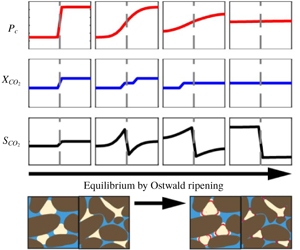
Results from the example case of the numerical simulation are presented in figure 3. During the early stages, a sharp gradient of  $\text{CO}_{2}$ capillary pressure and resulting
  $\text{CO}_{2}$ mass fraction gradient can be seen at the interface between the two domains. Here, the
  $\text{CO}_{2}$ mass fraction in the aqueous phase
  $X$ is defined as
 $$\begin{eqnarray}X={\displaystyle \frac{\text{mass of dissolved }\text{CO}_{2}}{\text{mass of dissolved }\text{CO}_{2}+\text{mass of water}}}.\end{eqnarray}$$
 This mass fraction gradient initiates diffusion of  $\text{CO}_{2}$ in the aqueous phase from the high capillary pressure domain to the other. Over time, the gradients of
  $\text{CO}_{2}$ mass fraction and capillary pressure decrease, and
  $\text{CO}_{2}$ saturation redistributes between the two domains even though the separate-phase
  $\text{CO}_{2}$ is set to be immobile over the entire simulation period (e.g. the relative permeability is zero). The results show that Ostwald ripening is capable of changing the saturation distribution of
  $\text{CO}_{2}$ between the two domains.
For the example shown here, establishing equilibrium between the two domains requires a period of about 10 years, even though the domain size is very small (0.01 m).
Table 1. Simulation input parameters of the example case shown in figure 3.


Figure 3. An example of numerical simulation on redistributing residually trapped  $\text{CO}_{2}$ by Ostwald ripening in the aqueous phase. The evolution of (a) capillary pressure, (b)
  $\text{CO}_{2}$ mass fraction in the aqueous phase and (c)
  $\text{CO}_{2}$ saturation are shown. The
  $\text{CO}_{2}$ saturation increases in the low capillary pressure domain due to Ostwald ripening even though the separate-phase
  $\text{CO}_{2}$ is immobile.
3 Mathematical model for residual  $\text{CO}_{2}$ redistribution by Ostwald ripening

Numerical simulation shows that residual  $\text{CO}_{2}$ can be redistributed by Ostwald ripening even though the residual
  $\text{CO}_{2}$ is completely immobile. However, the redistribution by Ostwald ripening is extremely slow. The characteristic time for diffusion is usually expressed as
 $$\begin{eqnarray}t_{c}={\displaystyle \frac{l^{2}}{D}},\end{eqnarray}$$
 where  $l$ is the characteristic length of the model and
  $D$ is the diffusion coefficient. For a single-phase diffusion problem (only the aqueous phase and dissolved
  $\text{CO}_{2}$) with the same size of the numerical model shown in the last section, the characteristic time should be of the order of hours. However, the time to approach equilibrium for Ostwald ripening is about 10 years. In this section, we develop a mathematical model to explain the large difference between the single-phase diffusion problem and the Ostwald ripening problem. This model is expected to provide insights on the retardation of the equilibration, and assumptions will be made in this model to reduce complexity such as reducing variables to constants that have little impacts on the diffusion problem.
As shown in figure 1, the low capillary pressure domain (domain 1) is receiving the diffusive flux of  $\text{CO}_{2}$ from the high capillary pressure domain (domain 2). The diffusive flux is responsible for both the increase of
  $\text{CO}_{2}$ mass fraction in the aqueous phase and the growth of separate-phase
  $\text{CO}_{2}$. By assuming diffusion only, without any advection of the
  $\text{CO}_{2}$ phase, the mass conservation equation for
  $\text{CO}_{2}$ is
 $$\begin{eqnarray}{\displaystyle \frac{\unicode[STIX]{x2202}(XS_{w}\unicode[STIX]{x1D70C}_{w}\unicode[STIX]{x1D719})}{\unicode[STIX]{x2202}t}}+{\displaystyle \frac{\unicode[STIX]{x2202}(YS_{g}\unicode[STIX]{x1D70C}_{g}\unicode[STIX]{x1D719})}{\unicode[STIX]{x2202}t}}={\displaystyle \frac{\unicode[STIX]{x2202}}{\unicode[STIX]{x2202}x}}\left[\unicode[STIX]{x1D719}D_{w}S_{w}{\displaystyle \frac{\unicode[STIX]{x2202}(X\unicode[STIX]{x1D70C}_{w})}{\unicode[STIX]{x2202}x}}\right],\end{eqnarray}$$
 where  $X$ and
  $Y$ are the
  $\text{CO}_{2}$ mass fractions in the aqueous phase and in the
  $\text{CO}_{2}$ phase, respectively,
  $S_{w}$ and
  $S_{g}$ are the water saturation and
  $\text{CO}_{2}$ saturation,
  $\unicode[STIX]{x1D70C}_{w}$ and
  $\unicode[STIX]{x1D70C}_{g}$ are the water density and
  $\text{CO}_{2}$ density, and
  $x$ is the distance. The term
  $\unicode[STIX]{x1D719}D_{w}S_{w}$ can be viewed as the effective diffusion coefficient accounting for the area open to diffusion.
Equation (3.2) can be simplified by assuming some variables are constants. First, the water density  $\unicode[STIX]{x1D70C}_{w}$,
  $\text{CO}_{2}$ density
  $\unicode[STIX]{x1D70C}_{g}$, diffusion coefficient
  $D_{w}$ and porosity
  $\unicode[STIX]{x1D719}$ can be assumed constant and equal to the values in domain 2 due to constant temperature and a negligible change of pressure during the evolution compared to reservoir pressure. Second, the
  $\text{CO}_{2}$ mass fraction in the gaseous phase
  $Y$ can be assumed to be equal to 1. Although
  $Y$ is a complex function of
  $X$ and local reservoir conditions as shown in equations 1 and 2 in Spycher & Pruess (Reference Spycher and Pruess2005), figure 2 of their paper shows that the water mole fraction in the
  $\text{CO}_{2}$ phase is near 1 %–2 % for reservoir conditions. Therefore,
  $Y$ can be expected to be larger than 99 %. Third, water saturation can be assumed to be 1 for simplicity. The first and second terms in (3.2) represent the
  $\text{CO}_{2}$ mass in the aqueous phase and in the
  $\text{CO}_{2}$ phase, respectively. Considering
  $Y$ (around 99 %) is much larger than
  $X$ (around 5 %) (Spycher & Pruess Reference Spycher and Pruess2005) and there is a high saturation of residual
  $\text{CO}_{2}$ (Burnside & Naylor Reference Burnside and Naylor2014), the amount of
  $\text{CO}_{2}$ in the aqueous phase is significantly smaller than that in the
  $\text{CO}_{2}$ phase. Therefore, it is safe to assume that
  $S_{w}=1$ with minimal impact on the total amount of
  $\text{CO}_{2}$ in the system. Based on the above assumptions, equation (3.2) becomes
 $$\begin{eqnarray}{\displaystyle \frac{\unicode[STIX]{x2202}X}{\unicode[STIX]{x2202}t}}+{\displaystyle \frac{\unicode[STIX]{x1D70C}_{g}}{\unicode[STIX]{x1D70C}_{w}}}{\displaystyle \frac{\unicode[STIX]{x2202}S_{g}}{\unicode[STIX]{x2202}t}}=D_{w}{\displaystyle \frac{\unicode[STIX]{x2202}^{2}X}{\unicode[STIX]{x2202}x^{2}}}.\end{eqnarray}$$
 Changes in  $S_{g}$ can be expressed as a function of changes in local
  $\text{CO}_{2}$ mass fraction
  $X$ by
 $$\begin{eqnarray}{\displaystyle \frac{\unicode[STIX]{x2202}S_{g}}{\unicode[STIX]{x2202}t}}={\displaystyle \frac{\text{d}S_{g}}{\text{d}P_{c}}}{\displaystyle \frac{\text{d}P_{c}}{\text{d}X}}{\displaystyle \frac{\unicode[STIX]{x2202}X}{\unicode[STIX]{x2202}t}}.\end{eqnarray}$$
 In (3.4) the term  $\text{d}S_{g}/\text{d}P_{c}$ can be calculated from the capillary pressure model for the rock. The term
  $\text{d}P_{c}/\text{d}X$ can be estimated based on the data from Spycher & Pruess (Reference Spycher and Pruess2005) for specific reservoir conditions. Detailed estimation of this term will be described in the following section.
Substituting (3.4) into (3.3), equation (3.3) can be written in the form
 $$\begin{eqnarray}R_{CO_{2}}{\displaystyle \frac{\unicode[STIX]{x2202}X}{\unicode[STIX]{x2202}t}}=D_{w}{\displaystyle \frac{\unicode[STIX]{x2202}^{2}X}{\unicode[STIX]{x2202}x^{2}}},\end{eqnarray}$$
where
 $$\begin{eqnarray}R_{CO_{2}}=1+{\displaystyle \frac{\unicode[STIX]{x1D70C}_{g}}{\unicode[STIX]{x1D70C}_{w}}}{\displaystyle \frac{\text{d}S_{g}}{\text{d}P_{c}}}{\displaystyle \frac{\text{d}P_{c}}{\text{d}X}}.\end{eqnarray}$$
 Here,  $R_{CO_{2}}$ is analogous to the concept of the ‘retardation factor’ commonly used in convection–dispersion problems with absorptive materials where the advance of the solute is retarded due to adsorption of the solute onto the matrix (Bear Reference Bear2013). The term
  $(\unicode[STIX]{x1D70C}_{g}/\unicode[STIX]{x1D70C}_{w})(\text{d}S_{g}/\text{d}P_{c})(\text{d}P_{c}/\text{d}X)$ is equivalent to the ‘adsorption’ term that retards the progress of
  $\text{CO}_{2}$ diffusion in the aqueous phase by absorbing
  $\text{CO}_{2}$ into the
  $\text{CO}_{2}$ phase. The time scale of residual
  $\text{CO}_{2}$ redistribution by Ostwald ripening can be estimated based on the time scale of the retarded diffusion process, such as the magnitude of
  $R_{CO_{2}}$.
To summarize, the mathematical model of residual  $\text{CO}_{2}$ distribution by Ostwald ripening can be expressed by re-arranging equation (3.5) to give
 $$\begin{eqnarray}{\displaystyle \frac{\unicode[STIX]{x2202}X}{\unicode[STIX]{x2202}t}}=D_{equiv}{\displaystyle \frac{\unicode[STIX]{x2202}^{2}X}{\unicode[STIX]{x2202}x^{2}}},\end{eqnarray}$$
with the equivalent diffusion coefficient
 $$\begin{eqnarray}D_{equiv}={\displaystyle \frac{D_{w}}{R_{CO_{2}}}}.\end{eqnarray}$$
4 Exact solution for Ostwald ripening in a homogeneous system and characteristic time
4.1 Exact solution for Ostwald ripening in a homogeneous system
Equations in the form of (3.7) have been solved extensively for particular representations of  $D_{equiv}$ (Fokas & Yortsos Reference Fokas and Yortsos1982; Kashchiev & Firoozabadi Reference Kashchiev and Firoozabadi2003). However, the problem we are interested in for this paper is defined as a two-domain system with different capillary pressure curves in each domain. This situation may cause the term
  $\text{d}S_{g}/\text{d}P_{c}$ in the diffusion coefficient to be in nonlinear and discontinuous forms that make the differential equation non-solvable. Therefore, we define a homogeneous system to illustrate the Ostwald ripening process while preserving the key characteristics of the problem in a heterogeneous system.
The system is a one-dimensional homogeneous porous medium with length  $L$ with two closed boundaries. The initial condition is that the
  $\text{CO}_{2}$ saturation is non-zero in the left half of the system and 0 in the right half. The mass fraction in the aqueous phase in the right half of the system is set such that any increase in
  $\text{CO}_{2}$ will result in the formation of separate-phase
  $\text{CO}_{2}$. On the left-hand side, the separate-phase
  $\text{CO}_{2}$ is at the residual saturation and kept immobile over the entire evolution. Over time,
  $\text{CO}_{2}$ will diffuse from the left domain to the right through the aqueous phase, and
  $\text{CO}_{2}$ saturation in the two domains will approach the same value. The entire system shares the identical capillary pressure curve so that the equivalent diffusion coefficient is continuous. In figure 4 we illustrate the defined system at its initial condition and equilibrium state.

Figure 4. A conceptual illustration of a homogeneous case with a  $\text{CO}_{2}$-saturated aqueous phase and only one domain initially containing separate-phase
  $\text{CO}_{2}$. The system approaches equilibrium through diffusive flux of
  $\text{CO}_{2}$ in the aqueous phase transporting
  $\text{CO}_{2}$ to increase
  $\text{CO}_{2}$ saturation in the other domain. Eventually, the
  $\text{CO}_{2}$ saturation will approach the same at equilibrium.
To solve (3.7) and (3.8) for the above system, it is necessary to find a specific form of  $R_{CO_{2}}$. Firstly, the derivative
  $\text{d}P_{c}/\text{d}X$ can be estimated from the equation-of-state for the
  $\text{CO}_{2}$–water–NaCl system for each temperature and pressure. For example, it can be estimated from the tangent of the molar fraction-pressure curves at a temperature and near the reservoir pressure in figure 2 of Spycher & Pruess (Reference Spycher and Pruess2005). To make the estimation more convenient, the tangent can be linked to the reservoir condition. Define
 $$\begin{eqnarray}\displaystyle & \displaystyle H_{0}={\displaystyle \frac{P_{w}}{X_{0}}}, & \displaystyle\end{eqnarray}$$
 $$\begin{eqnarray}\displaystyle & \displaystyle H_{tangent}={\displaystyle \frac{\text{d}P_{c}}{\text{d}X}}, & \displaystyle\end{eqnarray}$$
 where  $X_{0}$ denotes the background saturated
  $\text{CO}_{2}$ mass fraction. The derivative can be expressed by the reservoir condition through
 $$\begin{eqnarray}{\displaystyle \frac{\text{d}P_{c}}{\text{d}X}}={\displaystyle \frac{P_{w}}{X_{0}}}{\displaystyle \frac{H_{tangent}}{H_{0}}}.\end{eqnarray}$$
 The values of the ratio  $H_{tangent}/H_{0}$ can be found by interpolating figure 5 within a range of typical reservoir conditions for
  $\text{CO}_{2}$ sequestration. These values are generated by the equation-of-state ECO2N developed by Spycher & Pruess (Reference Spycher and Pruess2005).

Figure 5. Values of  $H_{tangent}/H_{0}$ between 12 and 18 MPa and 55 and
  $95\,^{\circ }\text{C}$.
Secondly, the derivative  $\text{d}S_{g}/\text{d}P_{c}$ can be found by assigning a specific form for the capillary pressure model, for example,
 $$\begin{eqnarray}P_{c}=a+bS_{g}^{c},\quad a\geqslant 0,\,b\neq 0,\,c\geqslant 1,\end{eqnarray}$$
 where  $a$,
$a$,  $b$ and
  $c$ are constants. The term
  $\text{d}S_{g}/\text{d}P_{c}$ can be written as
 $$\begin{eqnarray}{\displaystyle \frac{\text{d}S_{g}}{\text{d}P_{c}}}={\displaystyle \frac{1}{bc}}S_{g}^{1-c}.\end{eqnarray}$$
The retardation factor can be written as
 $$\begin{eqnarray}R_{CO_{2}}=1+{\displaystyle \frac{\unicode[STIX]{x1D70C}_{g}}{\unicode[STIX]{x1D70C}_{w}}}{\displaystyle \frac{P_{w}}{X_{0}}}{\displaystyle \frac{H_{tangent}}{H_{0}}}{\displaystyle \frac{1}{bc}}S_{g}^{1-c}.\end{eqnarray}$$
 Here, we consider a special case where  $c=1$. The capillary pressure model becomes linear. The retardation factor becomes
 $$\begin{eqnarray}R_{CO_{2}}=1+{\displaystyle \frac{\unicode[STIX]{x1D70C}_{g}}{\unicode[STIX]{x1D70C}_{w}}}{\displaystyle \frac{P_{w}}{X_{0}}}{\displaystyle \frac{H_{tangent}}{H_{0}}}{\displaystyle \frac{1}{b}},\end{eqnarray}$$
and the equivalent diffusion coefficient becomes a constant, i.e.
 $$\begin{eqnarray}D_{equiv}={\displaystyle \frac{D_{w}}{1+{\displaystyle \frac{\unicode[STIX]{x1D70C}_{g}}{\unicode[STIX]{x1D70C}_{w}}}{\displaystyle \frac{P_{w}}{X_{0}}}{\displaystyle \frac{H_{tangent}}{H_{0}}}{\displaystyle \frac{1}{b}}}}.\end{eqnarray}$$
The boundary conditions and initial conditions are defined as
 $$\begin{eqnarray}\displaystyle & \displaystyle {\displaystyle \frac{\unicode[STIX]{x2202}X}{\unicode[STIX]{x2202}x}}\left(x=-{\displaystyle \frac{L}{2}},t\right)=0, & \displaystyle\end{eqnarray}$$
 $$\begin{eqnarray}\displaystyle & \displaystyle {\displaystyle \frac{\unicode[STIX]{x2202}X}{\unicode[STIX]{x2202}x}}\left(x={\displaystyle \frac{L}{2}},t\right)=0, & \displaystyle\end{eqnarray}$$
 $$\begin{eqnarray}\displaystyle & \displaystyle X\left(-{\displaystyle \frac{L}{2}}<x\leqslant 0,t=0\right)=X_{1}, & \displaystyle\end{eqnarray}$$
 $$\begin{eqnarray}\displaystyle & \displaystyle X\left(0<x\leqslant {\displaystyle \frac{L}{2}},t=0\right)=X_{0}, & \displaystyle\end{eqnarray}$$
 where  $X_{1}$ is the saturated
  $\text{CO}_{2}$ mass fraction at
  $P_{w}+P_{c_{1}}$, with the subscript 1 denoting the domain where the initial
  $\text{CO}_{2}$ saturation is non-zero. The exact solution to (3.7) is given by equation (2.17) in Crank (Reference Crank1975):
 $$\begin{eqnarray}X(x,t)-X_{0}={\displaystyle \frac{1}{2}}(X_{c1}-X_{0})\mathop{\sum }_{n=-\infty }^{\infty }\left\{erf{\displaystyle \frac{L/2+2nL-x}{2\sqrt{D_{equiv}t}}}+erf{\displaystyle \frac{L/2-2nL+x}{2\sqrt{D_{equiv}t}}}\right\}.\end{eqnarray}$$
 The  $\text{CO}_{2}$ saturation can be computed by combining (3.4) and (4.5),
 $$\begin{eqnarray}S_{g}={\displaystyle \frac{\text{d}P_{c}}{\text{d}X}}{\displaystyle \frac{X-X_{0}}{b}}.\end{eqnarray}$$
 In figure 6 we compare the exact solution with detailed numerical simulation of an example homogeneous case. The results of the numerical solution achieve a close agreement with the exact solution. The slight deviation may result from the nonlinearity of the capillary pressure– $\text{CO}_{2}$ mass fraction relationship and pressure redistribution during the evolution. The time scale of equilibration is over ten years.

Figure 6. The comparison of the exact solution and detailed numerical simulation on an homogeneous case. The two results achieve close agreement. The reservoir condition is at 15 MPa and  $75\,^{\circ }\text{C}$. The initial
  $\text{CO}_{2}$ saturation is 0.4 in the left half of the system. The capillary pressure model is
  $P_{c}=3000S_{g}$.
4.2 Characteristic time of Ostwald ripening
The characteristic times of a single-phase diffusion problem and a two-phase diffusion problem discussed above are
 $$\begin{eqnarray}\displaystyle & \displaystyle t_{c,single\text{-}phase}={\displaystyle \frac{l^{2}}{D_{w}}}, & \displaystyle\end{eqnarray}$$
 $$\begin{eqnarray}\displaystyle & \displaystyle t_{c,two\text{-}phase}={\displaystyle \frac{l^{2}}{D_{equiv}}}. & \displaystyle\end{eqnarray}$$
 Combining (3.8), the characteristic time of a two-phase diffusion problem (the aqueous phase and the  $\text{CO}_{2}$ phase) can be expressed as
 $$\begin{eqnarray}t_{c,two\text{-}phase}=R_{CO_{2}}t_{c,single\text{-}phase}.\end{eqnarray}$$
 Therefore, it is meaningful to figure out the order of magnitude of the retardation factor as shown in (4.7) to evaluate how the characteristic time changes when the separate-phase  $\text{CO}_{2}$ is involved. Firstly, the term
  $\unicode[STIX]{x1D70C}_{g}/\unicode[STIX]{x1D70C}_{w}$ is typically on the order of
  $10^{-1}$, where the
  $\text{CO}_{2}$ density is about several hundred
  $\text{kg}~\text{m}^{-3}$ and the water density is about
  $1000~\text{kg}~\text{m}^{-3}$ at reservoir conditions. Secondly, the term
  $P_{w}/X_{0}$ is of the order of
  $10^{9}$, where reservoir pressure
  $P_{w}$ is of the order of
  $10^{7}$ Pa and the
  $\text{CO}_{2}$ solubility in mass fraction
  $X_{0}$ is of the order of
  $10^{-2}.$ Thirdly, the term
  $H_{tangent}/H_{0}$ is of the order of 1 at reservoir conditions according to figure 5. Finally, the term
  $1/b$ is of the order of
  $10^{-3},$ where the capillary pressure values of sandstone typical for
  $\text{CO}_{2}$ sequestration is about several thousand Pascal when
  $\text{CO}_{2}$ saturation is close to residual saturation (Krevor et al. Reference Krevor, Pini, Zuo and Benson2012). Integrating all the above terms, the order of magnitude of the retardation factor is
 $$\begin{eqnarray}R_{CO_{2}}\sim (1+10^{-1}\times 10^{9}\times 1\times 10^{-3})\sim 10^{5}.\end{eqnarray}$$
 The large value for the retardation factor indicates that the existence of separate-phase  $\text{CO}_{2}$ significantly slows down the equilibration process, compared to single-phase problems. For example, taking the characteristic length of the heterogeneous system shown in figure 3 (0.005 m), the resulting characteristic time of a single-phase diffusion problem is 4600 s, which is around an hour. However, the characteristic time for the two-phase diffusion problem is increased by
  $10^{5}$, which is around 15 years. This estimation also agrees closely with the homogeneous case with an exact solution shown in figure 6. In general,
  $\text{CO}_{2}$ redistribution by Ostwald ripening can be expected to be a very slow process for typical reservoir properties.
5 Approximate solution for time scale estimation of residual $\text{CO}_{2}$ redistribution by Ostwald ripening in heterogeneous systems

The above sections discuss the mathematical model for residual  $\text{CO}_{2}$ redistribution by Ostwald ripening and the exact solution for a homogeneous system. In more general cases, the system is highly likely to be heterogeneous where the two adjacent domains are characterized by different capillary pressure curves. In this section, an approximate solution to estimate the time scale for Ostwald ripening is developed for heterogeneous systems.
5.1 Derivation of the approximate solution
The diffusive flux of  $\text{CO}_{2}$ in the aqueous phase
  $J$ can be written as
 $$\begin{eqnarray}J=-\unicode[STIX]{x1D70C}_{w}D_{w}{\displaystyle \frac{\unicode[STIX]{x2202}X}{\unicode[STIX]{x2202}x}}.\end{eqnarray}$$
 Assuming that the diffusion equation can be approximated by a step function at the interface between the two domains, the  $\text{CO}_{2}$ diffusive flux becomes
 $$\begin{eqnarray}J_{2\rightarrow 1}=\unicode[STIX]{x1D70C}_{w}D_{w}{\displaystyle \frac{X_{2}-X_{1}}{\unicode[STIX]{x1D6FC}L}},\end{eqnarray}$$
 where  $\unicode[STIX]{x1D6FC}$ is a scaling factor of the characteristic length
  $L$ with its value varying during equilibration. The term
  $\unicode[STIX]{x1D6FC}$ will be further defined in the next subsection. The subscripts 1 and 2 refer to the low capillary pressure domain and the high capillary pressure domains, respectively. This notation will be used throughout the derivation. The assumption of a step function achieves a first-order accuracy on predicting the diffusive flux. Since the main purpose of the approximate solution is to track the progress towards equilibrium between the two domains instead of capturing the accurate
  $\text{CO}_{2}$ saturation profile, this assumption is sufficient to serve such a purpose with reduced complexity.
The  $\text{CO}_{2}$ mass conservation equation for domain 1 is given by
 $$\begin{eqnarray}{\displaystyle \frac{\unicode[STIX]{x2202}(X_{1}S_{w1}\unicode[STIX]{x1D70C}_{w}\unicode[STIX]{x1D719}_{1}A_{c}L_{1})}{\unicode[STIX]{x2202}t}}+{\displaystyle \frac{\unicode[STIX]{x2202}(Y_{1}S_{g1}\unicode[STIX]{x1D70C}_{g}\unicode[STIX]{x1D719}_{1}A_{c}L_{1})}{\unicode[STIX]{x2202}t}}=AJ_{2\rightarrow 1},\end{eqnarray}$$
 where  $A_{c}$ is the cross-section area of the domain in the YZ plane and
  $A$ is the available cross-section area open to diffusion. The term
  $A$ is estimated by the harmonic mean of the two domains’ initially available area,
 $$\begin{eqnarray}A={\displaystyle \frac{2A_{c}}{{\displaystyle \frac{1}{\unicode[STIX]{x1D719}_{1}(1-S_{CO_{2},1}^{init})}}+{\displaystyle \frac{1}{\unicode[STIX]{x1D719}_{2}(1-S_{CO_{2},2}^{init})}}}},\end{eqnarray}$$
 where  $S_{CO_{2}}^{init}$ is the initial
  $\text{CO}_{2}$ saturation.
Similar assumptions discussed in § 3 are applied to the derivation here including  $Y_{1}=1$ and porosities and densities are constants. In addition, the rate of change of the
  $\text{CO}_{2}$ mass fraction in the aqueous phase is negligible because the supersaturation of the
  $\text{CO}_{2}$ mass fraction is only about
  $10^{-5}$ for such a slow process (figure 3). Combining (5.2) and (5.3) gives
 $$\begin{eqnarray}\unicode[STIX]{x1D70C}_{g}\unicode[STIX]{x1D719}_{1}L_{1}A_{c}{\displaystyle \frac{\unicode[STIX]{x2202}(S_{g1})}{\unicode[STIX]{x2202}t}}=A\unicode[STIX]{x1D70C}_{w}D_{w}{\displaystyle \frac{X_{2}-X_{1}}{\unicode[STIX]{x1D6FC}L}}.\end{eqnarray}$$
 The term  $X_{2}-X_{1}$ can be found by applying a first-order approximation to (4.3), yielding
 $$\begin{eqnarray}{\displaystyle \frac{P_{c2}(S_{CO_{2},2})-P_{c1}(S_{CO_{2},1})}{X_{2}-X_{1}}}={\displaystyle \frac{P_{w}}{X_{0}}}{\displaystyle \frac{H_{tangent}}{H_{0}}}.\end{eqnarray}$$
 Here, the capillary pressures  $P_{c1}$ and
  $P_{c2}$ are functions of
  $S_{CO_{2},2}$ and
  $S_{CO_{2},1}$, respectively. The
  $\text{CO}_{2}$ saturation in the two domains can be linked through a mass conservation equation by neglecting the concentration change in the aqueous phase, i.e.
 $$\begin{eqnarray}S_{CO_{2},1}^{init}\unicode[STIX]{x1D719}_{1}L_{1}+S_{CO_{2},2}^{init}\unicode[STIX]{x1D719}_{2}L_{2}=S_{CO_{2},1}\unicode[STIX]{x1D719}_{1}L_{1}+S_{CO_{2},2}\unicode[STIX]{x1D719}_{2}L_{2}.\end{eqnarray}$$
 This relationship holds over the course of the entire evolution. For simplicity, we choose that  $L_{1}=L_{2}=L/2$.
Therefore, the diffusion equation is reduced by combining equations (5.4)–(5.7) to give
 $$\begin{eqnarray}\displaystyle {\displaystyle \frac{\text{d}(S_{CO_{2},1})}{\text{d}t}} & = & \displaystyle {\displaystyle \frac{4\unicode[STIX]{x1D70C}_{w}D_{w}X_{0}H_{0}}{\left[{\displaystyle \frac{1}{\unicode[STIX]{x1D719}_{1}(1-S_{CO_{2},1}^{init})}}+{\displaystyle \frac{1}{\unicode[STIX]{x1D719}_{2}(1-S_{CO_{2},2}^{init})}}\right]\unicode[STIX]{x1D70C}_{g}\unicode[STIX]{x1D719}_{1}L^{2}\unicode[STIX]{x1D6FC}P_{w}H_{tangent}}}\nonumber\\ \displaystyle & & \displaystyle \times \{P_{c2}(S_{CO_{2},2}(S_{CO_{2},1}))-P_{c1}(S_{CO_{2},1})\}.\end{eqnarray}$$
 Finally, the equation can be solved by integrating (5.8) from the initial  $\text{CO}_{2}$ to any
  $\text{CO}_{2}$ saturation
  $S_{CO_{2},1}^{\ast }$ before equilibrium is achieved, i.e.
 $$\begin{eqnarray}\displaystyle t & = & \displaystyle {\displaystyle \frac{\left[{\displaystyle \frac{1}{\unicode[STIX]{x1D719}_{1}(1-S_{CO_{2},1}^{init})}}+{\displaystyle \frac{1}{\unicode[STIX]{x1D719}_{2}(1-S_{CO_{2},2}^{init})}}\right]\unicode[STIX]{x1D70C}_{g}\unicode[STIX]{x1D719}_{1}L^{2}\unicode[STIX]{x1D6FC}P_{w}H_{tangent}}{4\unicode[STIX]{x1D70C}_{w}D_{w}X_{0}H_{0}}}\nonumber\\ \displaystyle & & \displaystyle \times \,\int _{S_{CO_{2},1}^{init}}^{S_{CO_{2},1}^{\ast }}{\displaystyle \frac{1}{P_{c2}(S_{CO_{2},2}(S_{CO_{2},1}))-P_{c1}(S_{CO_{2},1})}}d(S_{CO_{2},1}).\end{eqnarray}$$
 Equation (5.9) is a complete form of the approximate solution. It predicts the time required for the  $\text{CO}_{2}$ saturation in domain 1 to evolve from
  $S_{CO_{2},1}^{init}$ to
  $S_{CO_{2},1}^{\ast }$ when the initial conditions and reservoir properties are known. The integration part in (5.9) can be solved by numerical integration or Taylor series. A complete form of the approximate solution by Taylor series is shown in (A 15) of appendix A. The value for the scaling factor
  $\unicode[STIX]{x1D6FC}$ is determined by simulation results in the following subsection.
5.2 Values of length scaling factor $\unicode[STIX]{x1D6FC}$

Although the initial and equilibrated  $\text{CO}_{2}$ saturation may vary from case to case over a wide range, all cases exhibit the same trend, that is, the capillary pressure gradient between the two domains declines from the initial value to zero. We define a term
  $F$ to represent the remaining fraction of the driving force, e.g. capillary pressure gradient, during equilibration as follows:
 $$\begin{eqnarray}F={\displaystyle \frac{P_{c2}(t)-P_{c1}(t)}{P_{c2}^{init}-P_{c2}^{init}}}.\end{eqnarray}$$
 Here,  $P_{c}^{init}$ is the initial capillary pressure in each domain and
  $P_{c}(t)$ is the capillary pressure at an arbitrary time
  $t$ during equilibration. The term
  $F$ represents the remaining capillary pressure gradient normalized by its initial gradient. It is an indication of the progress of the equilibration by demonstrating the decline of the driving force of Ostwald ripening. The value of
  $F$ is 1 at the beginning of the evolution and declines over time to 0 at equilibrium.
The value of  $\unicode[STIX]{x1D6FC}$ varies throughout the process of equilibration, and, thus, the scaled length
  $\unicode[STIX]{x1D6FC}L$ that the capillary pressure difference applies to varies over time. As can be observed in the numerical solutions shown in figures 3 and 6, the capillary pressure gradient is sharp at the boundary between the two domains at the early stages of equilibration, leading to a strong diffusive flux. At later stages, the capillary pressure gradient smears out as the capillary pressure becomes more uniform within each domain. Therefore, the parameter
  $\unicode[STIX]{x1D6FC}$ is adjusted to correct the diffusion length to take into consideration the strong diffusive flux at the early stages of equilibration.
Numerical simulation with various resolutions is performed to find a functional form for  $\unicode[STIX]{x1D6FC}$. A thousand cases with randomly sampled physical parameters are run with 2 grid cells and 16 grid cells respectively. The two-grid-cell cases correspond to the assumption of step function with no spatial variation within each domain and the 16-grid-cell cases correspond to cases with spatially resolved gradients. The value of
  $\unicode[STIX]{x1D6FC}$ can be found by numerical simulation based on the equation
 $$\begin{eqnarray}\unicode[STIX]{x1D6FC}(F)={\displaystyle \frac{t_{16-grid-cell}(F)}{t_{2-grid-cell}(F)}}\times 0.5,\end{eqnarray}$$
 where  $t_{16-grid-cell}(F)$ and
  $t_{2-grid-cell}(F)$ are the times required by a 2-grid-cell case and a 16-grid-cell case to evolve to a certain
  $F$. The number 0.5 denotes that the 2-grid-cell case takes the diffusion length to be
  $0.5L$. Here,
  $\unicode[STIX]{x1D6FC}$ is a function of
  $F$ that varies at different stages during equilibration.
In figure 7 we summarize  $\unicode[STIX]{x1D6FC}$ from the 1000 cases as a function of
  $F$. The value of
  $\unicode[STIX]{x1D6FC}$ starts out smaller than 0.5 and increases as the system evolves towards equilibrium. A fitted mean of
  $\unicode[STIX]{x1D6FC}$ is shown figure 7.

Figure 7. Values of  $\unicode[STIX]{x1D6FC}$ as a function of
  $F$. A total of 1000 simulations with 16 grid cells are summarized. A second-order polynomial function is fitted to the mean of
  $\unicode[STIX]{x1D6FC}$.
The capillary pressure gradient decline curves over time for the example case listed in table 1 are shown in figure 8. As shown in figure 8(a), grid sensitivity simulations indicate that the capillary pressure gradient declines faster in models with higher resolution. This is consistent with the fact that the capillary pressure gradient is initially very steep between the two domains. In figure 8(b) we show the capillary pressure decline curve predicted by the approximate solution with and without the corrected diffusion length by  $\unicode[STIX]{x1D6FC}$. Without the correction (
 $\unicode[STIX]{x1D6FC}=0.5$), the prediction of the approximate solution agrees well with the numerical solutions with two grid cells, corresponding to the assumption of step function. With correction by fitted mean of
  $\unicode[STIX]{x1D6FC}$, the approximate solution captures the time-varying diffusion length and, thus, achieves an excellent agreement with the numerical simulation with high resolution.

Figure 8. Capillary pressure decline curves of the example case shown in figure 3.
5.3 Validation of the approximate solution
The approximate solution is validated through comparison with detailed numerical simulations. To test the robustness of the solution, each physical parameter of a single case is randomly sampled from a wide range that is representative of geological  $\text{CO}_{2}$ storage parameters, as shown in table 2. Correlations of key physical parameters are shown in figure 9. A total of 1000 simulations are performed.
Table 2. Numerical simulation input parameters and ranges for sampling.


Figure 9. Input parameters and correlations for the 1000 runs used to test the approximate solution. (a) Porosity and permeability are positively correlated. (b) Entry pressure and permeability are negatively correlated. (c) The majority of cases have initial capillary pressure differences below 5000 Pa.

Figure 10. (a) The comparison of evolution time between numerical simulations with 16 grid cells and predictions by the approximate solution (5.9). The agreement is fairly close. (b) The relative error of time for the system to evolve to a range of  $F$ values. (c) The error of
  $F$ values predicted by the approximate solution and numerical simulation measured at a range of
  $F$ from numerical simulation.
In figure 10(a) we compare the simulation results from 1000 randomly sampled cases (performed with 16 grid cells) with predictions from the approximate solution at various values of  $F$. The agreement is excellent at both early and late stages of evolution. Errors are measured by the difference of capillary pressure decline curves predicted by the approximate solution and numerical simulation in both the horizontal and vertical directions. In figure 10(b) we measure the horizontal difference, which is the relative error of time for the system to evolve to a range of
  $F$ values. In figure 10(c) we measure the vertical difference, which is the difference between
  $F$ predicted by the solution and numerical simulation. The lower and upper quartile of both errors are within
  $\pm 0.02$, indicating that the approximate solution achieves a close agreement with numerical simulation.
6 Discussion
6.1 Implications for the long-term fate of residual $\text{CO}_{2}$

We have demonstrated and quantified the time scale for a new mechanism for redistribution of residually trapped  $\text{CO}_{2}$ due to reservoir heterogeneity. The
  $\text{CO}_{2}$ saturations will increase in portions of the rocks with lower capillary pressure and decrease in those with higher capillary pressures. Such are the conditions expected to be present after imbibition of reservoir brine into the
  $\text{CO}_{2}$ plume during the post-injection period. As shown in figure 11, for millimeter-scale systems, the time scale of mass redistribution ranges from days to years, varying by several orders of magnitude depending on the total mass of
  $\text{CO}_{2}$, capillary heterogeneity and reservoir conditions. The time scale increases with the increase of model size
  $L$ following a power law (
 ${\sim}L^{2}$), such that a metre-scale model may take thousands of years or more to redistribute residually trapped
  $\text{CO}_{2}$.

Figure 11. The time scale of residual  $\text{CO}_{2}$ redistribution by Ostwald ripening within a range of model sizes at selected
  $F$ values. The results are predicted by the approximate solution and validated by numerical simulation. The time scale of redistribution increases with the increase of model size (
 ${\sim}L^{2}$). For example, millimetre-scale models may have an evolution time scale ranging from months to years. Models over metre scales may take thousands of years or longer to equilibrate.
The time period for continuum-scale Ostwald ripening depends on the nature of the capillary pressure curves during redistribution of the  $\text{CO}_{2}$. We have assumed particular parametric forms for these curves, based on a plausible understanding of the pore-scale processes that are occurring. To date, there are no direct measurements of the capillary pressure curves during Ostwald ripening. It would be valuable to make these measurements to include them in model calculations. This would be a challenging but worthwhile pursuit, ideally done by combining both pore-scale and continuum-scale measurements. In addition, we assume that the relative permeability to
  $\text{CO}_{2}$ phase is zero for all times and throughout both domains. For the domain with increasing saturations, it is certainly possible that the
  $\text{CO}_{2}$ phase would become mobile. If this occurs, we would expect that Ostwald ripening would be slightly faster, due to the redistribution of
  $\text{CO}_{2}$ away from the interface between the two domains.
This study seeks to evaluate the impact of Ostwald ripening on trapped  $\text{CO}_{2}$, and, thus, geological gradients other than the capillary pressure gradient such as pressure gradients by regional flow and other potential mechanisms of mass transfer in a geological storage site are neglected. In reality, other processes such as brine advection,
  $\text{CO}_{2}$ dissolution and mineralization will take place simultaneously. For example, advection and buoyancy-driven flows may increase the risk of remobilization of aggregated
  $\text{CO}_{2}$, while dissolution of trapped
  $\text{CO}_{2}$ may mitigate
  $\text{CO}_{2}$ aggregation by reducing the total amount of residually trapped
  $\text{CO}_{2}$. Coupling of these mechanisms would be another interesting topic that may affect the fate of trapped
  $\text{CO}_{2}$ significantly.
While this study has focused on the  $\text{CO}_{2}$–water system, it is equally applicable to other systems where the non-wetting phase is soluble in the wetting phase, for example, the methane–brine system. Hydrocarbon migration takes place on similar time scales to the processes described here, suggesting that Ostwald ripening due to reservoir heterogeneity may play a role in basin-scale gas migration.
6.2 Trend of capillary pressure of a shrinking $\text{CO}_{2}$ ganglion

The approximate solution and numerical simulation are developed with a monotonically decreasing capillary pressure model by assuming that the residual  $\text{CO}_{2}$ always attaches to the pore matrix during equilibration. It is likely that at some point, the
  $\text{CO}_{2}$ ganglion will become smaller than the pore body, no longer being supported by the pore walls. Once this occurs, the structure of the porous media no longer controls the capillary pressure because the ganglion will become a spherical bubble, resulting in an increase in curvature. At this point, as ripening proceeds, the capillary pressure will progressively increase as the bubble shrinks and disappears. In figure 12 we present a conceptual illustration of capillary pressure of a trapped ganglion including ganglion detachment from the pore walls. A minimum capillary pressure could exist near the saturation where detachment of ganglia may happen.
Some previous works have focused on exploring the impact on capillary pressure by the residual portion of the non-wetting phase by pore-network modelling. Conventionally, the capillary pressure curve constructed by experiments is only between the wetting phase and the continuous portion of the non-wetting phase, and the residual portion of the non-wetting phase is excluded from the measurement (Bear Reference Bear2013). McClure et al. (Reference McClure, Berrill, Gray and Miller2016) showed that the capillary pressure within a porous medium increases with an increasing number of ganglia and decreasing non-wetting phase saturation near low non-wetting phase saturations, resulting from detachment of non-wetting phase ganglia detachment from the pore walls. de Chalendar et al. (Reference de Chalendar, Garing and Benson2018) showed that the trend of capillary pressure of a single ganglion is opposite before and after detachment. These works imply that the trend of capillary pressure of the residual non-wetting phase could be altered due to ganglion detachment from the pore walls when the non-wetting phase saturation is small.
Our mathematical model does not explicitly include this last stage because it will be relevant only for scenarios where the non-wetting phase completely disappears from one of the domains. Even so, the consequence of excluding it will be that Ostwald ripening occurs faster than we predict in these late stages. In figure 13 we show three possible equilibrium states considering the upward trend of capillary pressure curves at low  $\text{CO}_{2}$ saturations. For this study, we assume that the initial condition for Ostwald ripening is at the end of imbibition and that all of the
  $\text{CO}_{2}$ ganglia are supported by pore walls. The equilibrium state is determined by both capillary pressure and mass conservation. Equilibrium state 1 corresponds to the case discussed in the approximate solution that the capillary pressures of the two domains reach equilibrium without any detachment. At equilibrium state 2, the capillary pressures reach equilibrium with the capillary pressure of one side going over the minimum value. At equilibrium state 3, the capillary pressure of the
  $\text{CO}_{2}$-discharging domain increases rapidly after detachment until separate-phase
  $\text{CO}_{2}$ is depleted.

Figure 12. A conceptual description of a capillary pressure curve for a shrinking ganglion due to Ostwald ripening. At the endpoint of the imbibition capillary pressure curve, the ganglion is trapped in the pore space with its interface extended into the pore throat. For regions where the  $\text{CO}_{2}$ saturation is decreasing, as Ostwald ripening progresses, the interface of the ganglion retreats from the pore throat towards the pore body. At some point, the ganglion may shrink and retreat fully into the pore body. Once the ganglion separates from the pore wall, we assume that since the rock is water-wet, the curvature corresponds to the radius of a spherical bubble and increases rapidly as the bubble shrinks and eventually disappears. The precise nature of the capillary pressure curve at this time is unknown, and the representation is provided here only for illustrative purposes. The rising trend of capillary pressure after ganglion detachment are illustrated in de Chalendar et al. (Reference de Chalendar, Garing and Benson2018) and McClure et al. (Reference McClure, Berrill, Gray and Miller2016).
In figure 13 we also show the evolution of the remaining driving force for Ostwald ripening during equilibration. At equilibrium state 2, it indicates that the ganglia in one domain are no longer supported by pore walls, but it is still possible for the capillary pressures of the two domains to approach the same value. Because the diffusive flux of  $\text{CO}_{2}$ is always from the high capillary pressure domain to the low capillary pressure domain, Ostwald ripening will still progress in the same direction as long as the direction of the capillary pressure gradient remains the same. At equilibrium state 3, after the capillary pressure of the high capillary pressure domain passes the minimum value, the capillary pressure gradient progressively increases in the same direction, which can accelerate diffusive transport between the two domains. The gradient may keep increasing until all of the separate-phase
  $\text{CO}_{2}$ is transported to the low capillary pressure domain. Therefore, Ostwald ripening can still progress in the same direction taking into consideration the detachment from the pore wall of shrinking ganglia and even be faster than predicted by the approximate solution due to increasing capillary pressure gradients. However, when and how the detachment of ganglia happen by Ostwald ripening in real-rock systems and how much Ostwald ripening can be accelerated is also an interesting research question to be explored further.

Figure 13. Examples of possible equilibrium states of Ostwald ripening based on capillary pressure curves with a rising trend near low  $\text{CO}_{2}$ saturation. The equilibrium state is determined by both capillary pressure curves and
  $\text{CO}_{2}$ mass conservation. Scenario 1: equilibrium at equal capillary pressure. Scenario 2: equilibrium at equal capillary pressure with one domain passing the minimum capillary pressure. Scenario 3: all of the separate-phase
  $\text{CO}_{2}$ in one domain is transported to the other.
7 Conclusions
This study proposed and investigated a new mechanism for mass redistribution of residually trapped supercritical  $\text{CO}_{2}$ within porous media with capillary heterogeneity. A new conceptual model, numerical simulation, and a new approximate solution were developed to demonstrate that Ostwald ripening, a pore-scale phenomenon, can result in continuum-scale redistribution of trapped
  $\text{CO}_{2}$. Increases in
  $\text{CO}_{2}$ saturation could potentially lead to remobilization of residually trapped
  $\text{CO}_{2}$.
An analogous retardation factor is derived to illustrate that the characteristic time for Ostwald ripening is of the order of  $10^{5}$ times slower than a single-phase diffusion problem due to the existence of separate-phase
  $\text{CO}_{2}$. An approximate solution for predicting the time scale of the mass redistribution due to Ostwald ripening was developed and validated through numerical simulation over a wide range of parameters that covered typical conditions for a geological storage site. Results showed that for millimetre-scale spatial domains, redistribution and capillary equilibration can occur on the time scale of months to years. For metre-scale systems, redistribution is very slow, requiring 10 000 years and longer. Although
  $\text{CO}_{2}$ redistribution by Ostwald ripening is a fairly slow process and seems to have little impact at the reservoir scale, at small spatial scales it can occur quickly. Understanding the implications of this process on long-term plume evolution will require consideration of the complex interplay of viscous, buoyancy and capillary forces, along with dissolution of the
  $\text{CO}_{2}$ into reservoir brine due to convective mixing or regional groundwater flow.
Acknowledgements
This study was funded by the Global Climate and Energy Project. We thank faculty members and students in the Department of Energy Resources Engineering for inspiring discussions and thoughtful opinions.
Declaration of interests
The authors report no conflict of interest.
Appendix A
To solve the integration part of the approximate solution, Taylor series can be applied to achieve a close estimation. The integration part of the approximate solution is
 $$\begin{eqnarray}\int _{S_{CO_{2},1}^{init}}^{S_{CO_{2},1}^{\ast }}{\displaystyle \frac{1}{P_{c2}(S_{CO_{2},2})-P_{c1}(S_{CO_{2},1})}}d(S_{CO_{2},1}).\end{eqnarray}$$
Define
 $$\begin{eqnarray}f(S_{CO_{2},1})={\displaystyle \frac{1}{P_{c2}(S_{CO_{2},2})-P_{c1}(S_{CO_{2},1})}}.\end{eqnarray}$$
Capillary pressure is represented by
 $$\begin{eqnarray}P_{c1}=P_{e1}+P_{01}\left({\displaystyle \frac{1-S_{wi,1}}{S_{CO_{2},1}}}-1\right)^{-(1/\unicode[STIX]{x1D706}_{1})}\end{eqnarray}$$
and
 $$\begin{eqnarray}P_{c2}=P_{e2}+P_{02}\left({\displaystyle \frac{1-S_{wi,2}}{S_{CO_{2},2}}}-1\right)^{-(1/\unicode[STIX]{x1D706}_{2})}.\end{eqnarray}$$
 The relationship of  $S_{CO_{2},1}$ and
  $S_{CO_{2},2}$ can be acquired from (5.7) as follows:
 $$\begin{eqnarray}S_{CO_{2},2}=aS_{CO_{2},1}+b.\end{eqnarray}$$
Here,
 $$\begin{eqnarray}a=-{\displaystyle \frac{\unicode[STIX]{x1D719}_{1}}{\unicode[STIX]{x1D719}_{2}}}\end{eqnarray}$$
and
 $$\begin{eqnarray}b={\displaystyle \frac{\unicode[STIX]{x1D719}_{1}}{\unicode[STIX]{x1D719}_{2}}}S_{CO_{2},1}^{init}+S_{CO_{2},2}^{init}.\end{eqnarray}$$
Therefore, (A 2) can be written as
 $$\begin{eqnarray}f(S_{CO_{2},1})={\displaystyle \frac{1}{P_{e2}+P_{02}\left({\displaystyle \frac{1-S_{wi,2}}{aS_{CO_{2},1}+b}}-1\right)^{-(1/\unicode[STIX]{x1D706}_{2})}-P_{e1}-P_{01}\left({\displaystyle \frac{1-S_{wi,1}}{S_{CO_{2},1}}}-1\right)^{-(1/\unicode[STIX]{x1D706}_{1})}}}.\end{eqnarray}$$
 Writing (A 8) in the form of a Taylor series evaluated at  $S_{0}$, we obtain
 $$\begin{eqnarray}f(S_{CO_{2},1})=f(S_{0})+f^{\prime }(S_{0})(S_{CO_{2},1}-S_{0})+{\displaystyle \frac{f^{\prime \prime }(S_{0})}{2}}(S_{CO_{2},1}-S_{0})^{2},\end{eqnarray}$$
where
 $$\begin{eqnarray}S_{0}=0.5(S_{CO_{2},1}^{init}+S_{CO_{2},1}^{eq}).\end{eqnarray}$$
 The term  $S_{CO_{2},1}^{eq}$ can be solved by equating the right-hand side of (A 3) and (A 4) and combining (5.7).
Write out the three terms about  $f(S_{0})$:
 $$\begin{eqnarray}\displaystyle \hspace{-24.0pt}f(S_{0}) & = & \displaystyle {\displaystyle \frac{1}{P_{e2}+P_{02}\left({\displaystyle \frac{1-S_{wi,2}}{aS_{0}+b}}-1\right)^{-(1/\unicode[STIX]{x1D706}_{2})}-P_{e1}-P_{01}\left({\displaystyle \frac{1-S_{wi,1}}{S_{0}}}-1\right)^{-(1/\unicode[STIX]{x1D706}_{1})}}},\end{eqnarray}$$
 $$\begin{eqnarray}\displaystyle \hspace{-24.0pt}f^{\prime }(S_{0}) & = & \displaystyle -[f(S_{0})]^{2}\left[{\displaystyle \frac{aP_{02}(1-S_{wi,2})}{\unicode[STIX]{x1D706}_{2}(aS_{0}+b)^{2}}}\left({\displaystyle \frac{1-S_{wi,2}}{aS_{0}+b}}-1\right)^{-(1/\unicode[STIX]{x1D706}_{2})-1}\right.\nonumber\\ \displaystyle \hspace{-24.0pt} & & \displaystyle \left.-\,{\displaystyle \frac{P_{01}(1-S_{wi,1})}{\unicode[STIX]{x1D706}_{1}S_{0}^{2}}}\left({\displaystyle \frac{1-S_{wi,1}}{S_{0}}}-1\right)^{-(1/\unicode[STIX]{x1D706}_{1})-1}\right],\end{eqnarray}$$
 $$\begin{eqnarray}\displaystyle \hspace{-24.0pt}f^{\prime \prime }(S_{0}) & = & \displaystyle {\displaystyle \frac{2[f^{\prime }(S_{0})]^{2}}{f(S_{0})}}-[f(S_{0})]^{2}\left[-{\displaystyle \frac{2a^{2}P_{02}(1-S_{wi,2})}{\unicode[STIX]{x1D706}_{2}(aS_{0}+b)^{3}}}\left({\displaystyle \frac{1-S_{wi,2}}{aS_{0}+b}}-1\right)^{-(1/\unicode[STIX]{x1D706}_{2})-1}\right.\nonumber\\ \displaystyle \hspace{-24.0pt} & & \displaystyle +\,{\displaystyle \frac{a^{2}P_{02}(1-S_{wi,2})^{2}(1+\unicode[STIX]{x1D706}_{2})}{\unicode[STIX]{x1D706}_{2}^{2}(aS_{0}+b)^{4}}}\left({\displaystyle \frac{1-S_{wi,2}}{aS_{0}+b}}-1\right)^{-(1/\unicode[STIX]{x1D706}_{2})-2}\nonumber\\ \displaystyle \hspace{-24.0pt} & & \displaystyle +\,{\displaystyle \frac{2P_{01}(1-S_{wi,1})}{\unicode[STIX]{x1D706}_{1}S_{0}^{3}}}\left({\displaystyle \frac{1-S_{wi,1}}{S_{0}}}-1\right)^{-(1/\unicode[STIX]{x1D706}_{1})-1}\nonumber\\ \displaystyle \hspace{-24.0pt} & & \displaystyle \left.-\,{\displaystyle \frac{(1-S_{wi,1})^{2}P_{01}(1+\unicode[STIX]{x1D706}_{1})}{\unicode[STIX]{x1D706}_{1}^{2}S_{0}^{4}}}\left({\displaystyle \frac{1-S_{wi,1}}{S_{0}}}-1\right)^{-(1/\unicode[STIX]{x1D706}_{1})-2}\right].\end{eqnarray}$$
Therefore, the integration can be written in the following form:
 $$\begin{eqnarray}\displaystyle & & \displaystyle \int _{S_{CO_{2},1}^{init}}^{S_{CO_{2},1}^{\ast }}{\displaystyle \frac{1}{P_{c2}(S_{CO_{2},2})-P_{c1}(S_{CO_{2},1})}}d(S_{CO_{2},1})\nonumber\\ \displaystyle & & \displaystyle \quad =\int _{S_{CO_{2},1}^{init}}^{S_{CO_{2},1}^{\ast }}f(S_{CO_{2},1})d(S_{CO_{2},1})\nonumber\\ \displaystyle & & \displaystyle \quad =\left[f(S_{0})S_{CO_{2},1}+f^{\prime }(S_{0})\left({\displaystyle \frac{1}{2}}S_{CO_{2},1}^{2}-S_{0}S_{CO_{2},1}\right)\right.\nonumber\\ \displaystyle & & \displaystyle \qquad +\,\left.{\displaystyle \frac{f^{\prime \prime }(S_{0})}{2}}\left({\displaystyle \frac{1}{3}}S_{CO_{2},1}^{3}-S_{0}S_{CO_{2},1}^{2}+S_{0}^{2}S_{CO_{2},1}\right)\right]\Bigg|_{S_{CO_{2},1}^{init}}^{S_{CO_{2},1}^{\ast }}\nonumber\\ \displaystyle & & \displaystyle \quad =\left[f(S_{0})S_{CO_{2},1}^{\ast }+f^{\prime }(S_{0})\left({\displaystyle \frac{1}{2}}S_{CO_{2},1}^{\ast 2}-S_{0}S_{CO_{2},1}^{\ast }\right)\right.\nonumber\\ \displaystyle & & \displaystyle \qquad +\,\left.{\displaystyle \frac{f^{\prime \prime }(S_{0})}{2}}\left({\displaystyle \frac{1}{3}}S_{CO_{2},1}^{\ast 3}-S_{0}S_{CO_{2},1}^{\ast 2}+S_{0}^{2}S_{CO_{2},1}^{\ast }\right)\right]\nonumber\\ \displaystyle & & \displaystyle \qquad -\,\left[f(S_{0})S_{CO_{2},1}^{init}+f^{\prime }(S_{0})\left({\displaystyle \frac{1}{2}}S_{CO_{2},1}^{init2}-S_{0}S_{CO_{2},1}^{init}\right)\right.\nonumber\\ \displaystyle & & \displaystyle \qquad \left.+\,{\displaystyle \frac{f^{\prime \prime }(S_{0})}{2}}\left({\displaystyle \frac{1}{3}}S_{CO_{2},1}^{init3}-S_{0}S_{CO_{2},1}^{init2}+S_{0}^{2}S_{CO_{2},1}^{init}\right)\right].\end{eqnarray}$$
 To summarize, the complete form of the approximate solution by Taylor series evaluated at  $S_{0}=0.5(S_{CO_{2},1}^{init}+S_{CO_{2},1}^{eq})$ is
 $$\begin{eqnarray}\displaystyle t & = & \displaystyle {\displaystyle \frac{\left[{\displaystyle \frac{1}{\unicode[STIX]{x1D719}_{1}(1-S_{CO_{2},1}^{init})}}+{\displaystyle \frac{1}{\unicode[STIX]{x1D719}_{2}(1-S_{CO_{2},2}^{init})}}\right]\unicode[STIX]{x1D70C}_{g}\unicode[STIX]{x1D719}_{1}L^{2}\unicode[STIX]{x1D6FC}P_{w}H_{tangent}}{4\unicode[STIX]{x1D70C}_{w}D_{w}X_{0}H_{0}}}\nonumber\\ \displaystyle & & \displaystyle \times \,\left\{\left[f(S_{0})S_{CO_{2},1}^{\ast }+f^{\prime }(S_{0})\left({\displaystyle \frac{1}{2}}S_{CO_{2},1}^{\ast 2}-S_{0}S_{CO_{2},1}^{\ast }\right)\right.\right.\nonumber\\ \displaystyle & & \displaystyle +\,\left.{\displaystyle \frac{f^{\prime \prime }(S_{0})}{2}}\left({\displaystyle \frac{1}{3}}S_{CO_{2},1}^{\ast 3}-S_{0}S_{CO_{2},1}^{\ast 2}+S_{0}^{2}S_{CO_{2},1}^{\ast }\right)\right]\nonumber\\ \displaystyle & & \displaystyle -\,\left[f(S_{0})S_{CO_{2},1}^{init}+f^{\prime }(S_{0})\left({\displaystyle \frac{1}{2}}S_{CO_{2},1}^{init2}-S_{0}S_{CO_{2},1}^{init}\right)\right.\nonumber\\ \displaystyle & & \displaystyle \left.\left.+\,{\displaystyle \frac{f^{\prime \prime }(S_{0})}{2}}\left({\displaystyle \frac{1}{3}}S_{CO_{2},1}^{init3}-S_{0}S_{CO_{2},1}^{init2}+S_{0}^{2}S_{CO_{2},1}^{init}\right)\right]\right\},\end{eqnarray}$$
 where  $f(S_{0})$,
  $f^{\prime }(S_{0})$ and
  $f^{\prime \prime }(S_{0})$ can be found using (A 11)–(A 13).


