


1. Introduction
The problem of particle–particle or particle–wall collisions in viscous fluids has important practical applications and has thus been the subject of a plethora of studies, not only experimental and numerical, but also from a purely mathematical standpoint. A precise understanding of both contact and near-to-contact dynamics would indeed have a profound impact on our understanding of complex phenomena such as sedimentation, filtration, lubrication and erosion (see, for example, Davis, Serayssol & Hinch Reference Davis, Serayssol and Hinch1986; Joseph Reference Joseph2003, and the references therein).
In spite of the attention it has received over the years, the problem is far from being fully resolved and the partial results which are available can often be counter-intuitive. An example is given by the simple case of a spherical rigid particle surrounded by a Stokes linear fluid that moves towards a wall. Indeed, it has been known for some time already that if both the particle and the wall are equipped with no-slip boundary conditions, contact cannot take place in a viscous incompressible fluid in finite time without singular forcing. We refer to Brenner (Reference Brenner1961) and Cooley & O'Neill (Reference Cooley and O'Neill1969) for some theoretical investigations based on singular perturbation techniques and formal asymptotic expansions. Since no-contact results are the starting point of this work, we highlight here some of the recent developments on this subject. A no-collision result for a simplified model in one space dimension for a fluid that obeys the viscous Burgers equation can be found in Vázquez & Zuazua (Reference Vázquez and Zuazua2006). No-contact results for an incompressible fluid modelled by the full Navier–Stokes equations were first obtained by Hesla (Reference Hesla2004) and Hillairet (Reference Hillairet2007) (see also Hillairet & Takahashi (Reference Hillairet and Takahashi2009) for extensions to the three-dimensional setting). The possible lack of collisions has been investigated in several different scenarios (see, for example, Hillairet, Seck & Sokhna (Reference Hillairet, Seck and Sokhna2018) for the case of a perfect Euler fluid and Grandmont & Hillairet (Reference Grandmont and Hillairet2016) for the case of a deformable beam-like structure). Despite the fact that in an incompressible fluid with no-slip boundary conditions contact seems to be impossible, it has been hypothesized that a particle can rebound provided that it is elastic, or in general, when it admits the storage and release of mechanical energy during the rebound, see e.g. Davis et al. (Reference Davis, Serayssol and Hinch1986). In view of these facts, the main question that motivated this work can be formulated as follows:
(Q.1) Can solid particles rebound inside a fluid in the absence of a topological contact?
In the following, we consider a smooth solid object (also referred to as particle or structure) that may be elastic or rigid and study its motion when thrown towards a rigid wall in a viscous incompressible liquid environment that adheres to all surfaces (that is, under no-slip boundary conditions). We consider both the two- and the three-dimensional cases. As remarked above, in this setting contact is excluded a priori (see Hesla Reference Hesla2004; Hillairet Reference Hillairet2007; Hillairet & Takahashi Reference Hillairet and Takahashi2009); indeed, it has been mathematically proven that the interplay of the regularity of all surfaces involved, the incompressibility of the fluid and the prescribed no-slip boundary conditions imply that a smooth, rigid body cannot reach any other smooth solid obstacle in finite time (for a numerical demonstration of this phenomenon in the case of a ball thrown towards a flat wall, see figure 4).
In this paper, we aim to advance the understanding of the extent to which the pathological behaviour described in the no-contact paradox can affect the dynamics of solid particles in close proximity to the boundary of the container. In particular, we are able to provide an affirmative answer to (Q.1) in a simplified setting (described in detail in § 2.3.2). To be precise, we investigate the rebound dynamics for body–fluid systems that allow for the following two features:
(i) The storage and release of mechanical energy to account for an elastic response of the solid; and
(ii) The possible deformations of the body. Especially the potential flattening of its boundary during the rebound phase.
While property (i) is a rather natural requirement, what is probably more peculiar is that (ii) turned out to significantly change the characteristic motion of the solid inside the fluid. As a matter of fact, what is possibly the most striking result of the paper is that if the shape is rigid then any eventual rebound of the particle becomes undetectable for sufficiently small values of the fluid viscosity (we make this precise in the statement of Theorem 1.1 below).
In the following we describe our two main results in more detail.
The simplified setting that is capable of capturing a rebound is motivated by our numerical experiments: we allow the fluid–solid interaction to affect the shape of the solid object – in particular its flatness. It is well understood (see, for example, the discussion in § 2.4 and the reference therein), that changes to the flatness of the particle in the nearest-to-contact region can have a significant influence on the magnitude of the drag force. Furthermore, since this effect becomes even more dramatic at small distances from other solid objects or from the boundary of the container, we tailor our model to adequately capture this interplay by considering a possible dependence on the deformation parameter in the damping term which represents the drag force. In this simplified setting (see Theorem 3.3), we show that rebound is indeed possible, provided that the solid experiences a substantial flattening of its near-to-contact region.
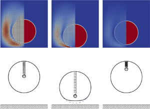
On the contrary, if the shape is rigid (that is, if (ii) is not satisfied), our investigation uncovers a rather surprising ‘trapping’ phenomenon for solids, thus providing further insight into the consequences of the no-contact paradox. In order to illustrate this effect, we study the motion of an object with rigid shape, which nevertheless allows for the storage and release of (a fraction of) its kinetic energy, as in property (i) above. As a model example, consider a rigid spherical shell with an internal mass–spring energy storing mechanism, as sketched in figure 1, thrown towards a flat wall. The expected dynamics for this particular configuration is as follows: as the outer shell is slowed down by the viscous forces preventing from collision, part of the kinetic energy of the system is stored in the inner mechanism; the shell can then be expected to rebound once this energy is transferred back to it by the upwards push applied by the mass–spring system. Moreover, one would also anticipate witnessing increasingly pronounced rebounds as friction in the fluid is reduced by considering gradually smaller values of the viscosity parameter. However, the analysis of this peculiar fluid–structure interaction performed on our reduced model predicts a rather different behaviour. This is made precise in the following result.
Theorem 1.1 In the vanishing viscosity limit, the rigid shell system described above moves freely (that is, as it would in the vacuum) towards the wall, to which it then sticks for all times after collision.

Figure 1. A spherical shell with an inner mass–spring system is surrounded by a viscous incompressible fluid.
For a proof of this result we refer the reader to § 3, and in particular to Theorem 3.2 below, where we show a more general result.
In view of Theorem 1.1, throughout the rest of the paper we say that a system does not produce a physical rebound if the distance between the body and the wall converges, in the vanishing viscosity limit, to a monotonically decreasing function of the time variable  $t$. Thus, for our purposes, a rebound is said to be physical (or physically meaningful) only if it withstands the vanishing viscosity limit in the sense above. It should be noted that the vanishing viscosity limit and the resulting limiting objects are used here as analytical tools to distinguish between different rebound behaviours (for more details, see Remark 3.5).
Since the models considered in Theorem 1.1 (and Theorem 3.2) yield solutions that do not withstand the vanishing viscosity limit, we conclude that some crucial aspect is missing in order to capture physical rebound effects: the motion described in Theorem 1.1 is not only in clear contrast with our real-world experience of bouncing objects, but also with laboratory experiments and numerical simulations (see, for example, the recent contributions of Hagemeier, Thévenin & Richter (Reference Hagemeier, Thévenin and Richter2021) and von Wahl et al. (Reference von Wahl, Richter, Frei and Hagemeier2020) or the experiments introduced in § 4). These observations naturally lead to the following question.
(Q.2) What is the mathematical reason for a physical rebound?
Our main contributions to this complicated issue are that we derive a reduced setting based on conditions (i) and (ii) for which we can prove the absence or the occurrence of a physical rebound. Further, we compare the reduced model with the classical partial differential equation (PDE) systems via numerical experiments. It turned out that, in the absence of topological contact, conditions (i) and (ii) are to some extent necessary and sufficient to obtain what we call a physically meaningful rebound. Further comparisons between reduced and PDE models via numerical experiments provide promising analogies. See indeed figure 10, where motions are compared for several values of the viscosity parameter. Consequently, our investigations and results prompted us to formulate the following conjecture on the qualitative conditions for rebounds.
Conjecture 1.2 A change in the flatness of the solid body as it approaches the wall, together with some elastic energy storage mechanism within the body, can potentially allow for a physically meaningful rebound (that is, that withstands the vanishing viscosity limit) even for no-slip boundary conditions preventing from topological contact.
While on the one hand the results presented in this paper (both analytical and numerical) allow us to speculate that our reduced model (conditions (i) and (ii)) could have indeed potentially captured the essential features of rebound in the absence of collisions, it should also be noted that a precise connection between the full PDE model and the reduced one is still missing. A full investigation of this issue is beyond the scope of this work. Actually, in the mathematical theory up to now, even the existence theory for bulk elastic solids interacting with fluids is rather sparse (see, for example, Grandmont Reference Grandmont2002; Benesova, Kampschulte & Schwarzacher Reference Benesova, Kampschulte and Schwarzacher2020). On the other hand, no-contact results for smooth deformable structures can be expected to be true, as indicated by Grandmont & Hillairet (Reference Grandmont and Hillairet2016). These results would offer a possible starting point for further mathematical investigations on rebound of elastic objects in viscous fluids. In regard to the further potential applicability of our mathematical theory, we put special effort into keeping the assumptions in the analytical section of the paper as general as possible, without, however, hindering the tractability of the reduced model. For this reason, in § 3.1 we provide an axiomatic set of assumptions which give the reduced model enough flexibility when it comes to fitting it with the full fluid–structure interaction (FSI) problem. Finally, we would like to point out that there has been a vast effort to study different mechanisms that allow for contact and possibly for a rebound. These include slip boundary conditions (Gérard-Varet & Hillairet Reference Gérard-Varet and Hillairet2014), the fluid compressibility (Feireisl Reference Feireisl2003, Reference Feireisl2004), pressure-dependent material properties (Barnocky & Davis Reference Barnocky and Davis1989), wall roughness (Gérard-Varet, Hillairet & Wang Reference Gérard-Varet, Hillairet and Wang2015), etc. (see also Joseph et al. Reference Joseph, Zenit, Hunt and Rosenwinkel2001; Joseph Reference Joseph2003 and the references therein). Moreover, some notions of weak solutions that allow for possible collisions have been considered by several authors (see, for example, Feireisl Reference Feireisl2004; Casanova, Grandmont & Hillairet Reference Casanova, Grandmont and Hillairet2021).
1.1. Structure of the paper
The paper is organized as follows. In § 2 we start by introducing the fluid–structure interaction model in the classical Eulerian–Lagrangian framework, which we then reformulate fully in the Eulerian setting, as needed for our numerical experiments. This is followed by the introduction of our reduced model of ordinary differential equations (ODEs). The section is closed by the derivation of drag formulas for the family of deformations that we consider for our numerical experiments and which form the model case for the analysis. § 3 is dedicated to the main mathematical results of this paper and their proofs. In § 3.1 we introduce our general assumptions and state the main theorems. In particular, we provide conditions that allow us to prove or disprove rebound in the vanishing viscosity limit. Section 3.2 is dedicated to the proofs of these results. In § 4, we first provide numerical experiments for the reduced model of ODEs. In the following subsection we introduce the numerical set-up that allows us to capture the bouncing behaviour of elastic solids for small viscosities and provide some numerical experiments. We conclude the section with the comparison from a numerical standpoint of the ODE and PDE solutions (see figure 10). Finally, in § 5 we summarize and discuss our results.
2. Modelling of particle–wall approach and rebound in viscous fluids
In this section, we first recall the standard Eulerian–Lagrangian formulation of the fluid–structure interaction problem, which we then reformulate in a purely Eulerian setting. This is followed by presenting a class of reduced ODE models for the FSI problem.
2.1. The viscous fluid – elastic structure Eulerian–Lagrangian formulation
Consider an incompressible Newtonian fluid filling the region  $\mathcal {F}(t)$, which surrounds an elastic particle whose position, at time
  $t$, will be denoted by
  $\mathcal {B}(t)$. We assume that the system composed of the fluid and the solid body occupies the region
  $\varOmega = \mathcal {F}(t) \cup \overline {\mathcal {B}(t)}$, where
  $\varOmega$ is an open subset of
  $\mathbb {R}^{N}$,
  $N = 2$ or
  $N = 3$. As is customary in fluid mechanics, the equations expressing the conservation of mass and the balance of linear momentum for the fluid are given in the Eulerian reference frame and read as follows:
 \begin{gather} \left. \begin{gathered}
\operatorname{div}_{\boldsymbol{x}} \boldsymbol{v} = 0,\\
\rho_f \left(\frac{\partial \boldsymbol{v}}{\partial t} +
\boldsymbol{v} \boldsymbol{\cdot}
\boldsymbol{\nabla}_{\boldsymbol{x}} \boldsymbol{v}\right)
= \operatorname{div}_{\boldsymbol{x}} \sigma_f + \rho_f
\boldsymbol{g}, \end{gathered} \quad \text{in }
\mathcal{F}(t),\!\right\} \end{gather}
\begin{gather} \left. \begin{gathered}
\operatorname{div}_{\boldsymbol{x}} \boldsymbol{v} = 0,\\
\rho_f \left(\frac{\partial \boldsymbol{v}}{\partial t} +
\boldsymbol{v} \boldsymbol{\cdot}
\boldsymbol{\nabla}_{\boldsymbol{x}} \boldsymbol{v}\right)
= \operatorname{div}_{\boldsymbol{x}} \sigma_f + \rho_f
\boldsymbol{g}, \end{gathered} \quad \text{in }
\mathcal{F}(t),\!\right\} \end{gather}
where  $\boldsymbol {v}(\boldsymbol {x},t)$ is the fluid velocity,
  $\rho _f$ is the constant fluid density and
  $\boldsymbol {g}(\boldsymbol {x},t)$ represents (Eulerian) external bulk accelerations. Here, the variable
  $\boldsymbol {x}$ denotes a position in the current (Eulerian) configuration, that is,
  $\boldsymbol {x} \in \mathcal {F}(t)$. We recall that for Newtonian fluids the Cauchy stress tensor
  $\sigma _f({\boldsymbol x},t)$ takes the form
 \begin{equation} \sigma_f ={-}p_f \boldsymbol{\mathsf{I}}_N + 2 \mu_f \boldsymbol{\mathsf{D}}(\boldsymbol{v}), \end{equation}
where  $p_f(\boldsymbol {x},t)$ denotes the fluid pressure,
  $\boldsymbol{\mathsf{I}}_N$ is the
  $N$-dimensional identity matrix,
  $\mu _f$ is the constant dynamic viscosity and
  $\boldsymbol{\mathsf{D}}(\boldsymbol {v}) \colon= (\boldsymbol {\nabla }_{\boldsymbol {x}} \boldsymbol {v} + (\boldsymbol {\nabla }_{\boldsymbol {x}} \boldsymbol {v})^\textrm {T})/2$ is the symmetric part of the gradient of
  $\boldsymbol {v}$. On the other hand, the balance equations for the elastic solid are given in the Lagrangian setting and can be written as
 \begin{equation} \left. \begin{aligned} \rho_s \frac{\partial^{2} \boldsymbol{\eta}}{\partial t^{2}} & = \operatorname{div}_{\boldsymbol{X}}\boldsymbol{\mathsf{P}} + \rho_s \boldsymbol{G},\\ J\rho_s & = \rho^{0}_s, \end{aligned} \quad \text{in } \mathcal{B}_0, \!\right\} \end{equation}
where  $\rho _s$ and
  $\rho _s^{0}$ denote the density of the elastic solid at time
  $t$ and in the reference configuration, respectively,
  $\boldsymbol {\eta }(\boldsymbol {X},t)$ is the displacement,
  $\boldsymbol{\mathsf{P}}(\boldsymbol {X},t)$ is the first Piola–Kirchhoff stress,
  $\boldsymbol {G}(\boldsymbol {X},t)$ is the (Lagrangian) external acceleration acting on the solid and
  $\mathcal {B}_0$ is the reference configuration of the solid. The variable
  $\boldsymbol {X}$ denotes a position in the reference (Lagrangian) configuration, that is,
  $\boldsymbol {X} \in \mathcal {B}_0$.
We assume that the structure is an incompressible hyperelastic solid, i.e.
 \begin{equation} \boldsymbol{\mathsf{P}} = \frac{\partial \mathcal{L}}{\partial \boldsymbol{\mathsf{F}}},\quad \text{where } \mathcal{L}(\boldsymbol{\mathsf{F}},P) \colon= \mathcal{W}(\boldsymbol{\mathsf{F}})-P(J-1). \end{equation}
Here,  $\mathcal {L}$ is the Lagrange function corresponding to the strain energy function
  $\mathcal {W}$ under the incompressibility restriction
  $J = 1$ and
  $P$ is the associated Lagrange multiplier. The symbol
  $\boldsymbol{\mathsf{F}}$ denotes the deformation gradient, i.e. if we define the deformation mapping
  $\boldsymbol {y}(\boldsymbol {X}, t) \colon= \boldsymbol {X} + \boldsymbol {\eta }(\boldsymbol {X}, t)$, then
 \begin{equation} \boldsymbol{\mathsf{F}}(\boldsymbol{X}, t) \colon= \boldsymbol{\nabla}_{\boldsymbol{X}}\boldsymbol{y}(\boldsymbol{X}, t) = \boldsymbol{\mathsf{I}}_N + \boldsymbol{\nabla}_{\boldsymbol X} \boldsymbol{\eta}(\boldsymbol{X},t). \end{equation}
Finally,  $J$ denotes the deformation gradient Jacobian, i.e.
  $J \colon= \mathrm {det}\,\boldsymbol{\mathsf{F}}$. Let us also mention here that, throughout the following, we assume that the deformation mapping
  $\boldsymbol {y}(\boldsymbol {\cdot }, t) \colon \mathcal {B}_0 \to \mathcal {B}(t)$ is a sufficiently smooth bijection for all
  $t$.
$t$.
The choice of the elastic material is determined by specifying the strain energy function  $\mathcal {W}$. As a particular example used later in the numerical computations (see § 4), we consider an incompressible neo-Hookean solid, for which the elastic strain energy is given by
 \begin{equation} \mathcal{W} \colon= \frac{G_s}{2}(|\boldsymbol{\mathsf{F}}|^{2}-N), \end{equation}
where the constant  $G_s$ denotes the shear modulus. The Cauchy stress in the solid can be expressed in terms of the first Piola–Kirchhoff stress
  $\boldsymbol{\mathsf{P}}$ as follows:
 \begin{equation} \sigma_s(\boldsymbol{x},t) = \left.\frac{1}{J({\boldsymbol X},t)}\boldsymbol{\mathsf{P}}({\boldsymbol X},t)\boldsymbol{\mathsf{F}}^{\rm T}({\boldsymbol X},t)\right|_{\boldsymbol{X} = \boldsymbol{y}^{{-}1}({\boldsymbol x},t)}. \end{equation}
As one can readily check, for the strain energy (2.6) the Cauchy stress in the solid takes the form
 \begin{equation} \sigma_s(\boldsymbol{x}, t) ={-}\tilde{p}(\boldsymbol{x}, t) \boldsymbol{\mathsf{I}}_N + G_s\boldsymbol{\mathsf{B}}(\boldsymbol{x}, t) ={-}p(\boldsymbol{x}, t)\boldsymbol{\mathsf{I}}_N + G_s\boldsymbol{\mathsf{B}}^{d}(\boldsymbol{x}, t), \end{equation}
where  $\tilde {p}(\boldsymbol {x},t)\colon= P(\boldsymbol {y}^{-1}({\boldsymbol x},t),t)$,
  $\boldsymbol{\mathsf{B}}(\boldsymbol {x},t)$ is the left Cauchy–Green tensor, which is classically defined via
 \begin{equation} \boldsymbol{\mathsf{B}}(\boldsymbol{x},t)\colon= \left.\boldsymbol{\mathsf{F}}(\boldsymbol{X}, t)\boldsymbol{\mathsf{F}}^{\rm T}(\boldsymbol{X}, t)\right|_{\boldsymbol{X} = \boldsymbol{y}^{{-}1}({\boldsymbol x},t)}, \end{equation}
the symbol  $\boldsymbol{\mathsf{B}}^{d} \colon= \boldsymbol{\mathsf{B}}-(1/N)(\operatorname {Tr}\boldsymbol{\mathsf{B}})\boldsymbol{\mathsf{I}}_N$ denotes its deviatoric part, and finally
  $p \colon= \tilde {p}-(1/N)\operatorname {Tr}\boldsymbol{\mathsf{B}}$.
The conditions describing the interaction between the fluid and the solid comprise the continuity of the velocities and of the tractions
 \begin{equation} \left. \begin{aligned} \boldsymbol{v}(\boldsymbol{x},t) & = \left.\frac{\partial \boldsymbol{\eta}(\boldsymbol{X},t)}{\partial t}\right|_{\boldsymbol{X}=\boldsymbol{y}^{{-}1}({\boldsymbol x},t)},\\ \sigma_f \boldsymbol{n} & = \sigma_s \boldsymbol{n}, \end{aligned} \quad \text{on } \partial \mathcal{B}(t), \!\right\} \end{equation}
where  $\boldsymbol {n}$ is the unit normal to the fluid–solid interface. Finally, we prescribe no-slip boundary conditions on the boundary of the domain, that is,
 \begin{equation} \boldsymbol{v} = \boldsymbol{0}, \quad \text{on } \partial \varOmega. \end{equation}
Note that the above system is a well posed problem for the unknowns  $\boldsymbol {v}, p$ describing the fluid in their variable-in-time Eulerian domain of definition and the deformation
  ${\boldsymbol {\eta }}$ and the pressure of the solid
  $P$ given in their steady Lagrangian coordinates. Moreover, it admits a formal energy equality (derived for the reader's convenience in Appendix B) of the following form:
 $$\begin{gather} \mathcal{K}(t) + \int_{\mathcal{B}_0} \mathcal{W}(\boldsymbol{X}, t)\,{\rm d}\boldsymbol{X} + \int_0^{t} \int_{\mathcal{F}(s)} 2 \mu_f |\boldsymbol{\mathsf{D}}(\boldsymbol{v}(\boldsymbol{x},s))|^{2} \,{\rm d}\kern0.7pt\boldsymbol{x} \,{\rm d}s = \mathcal{K}(0) + \int_{\mathcal{B}_0} \mathcal{W}(\boldsymbol{X}, 0)\,{\rm d}\boldsymbol{X}\nonumber\\ + \int_0^{t}\int_{\mathcal{F}(s)}\rho_f \boldsymbol{g}(\boldsymbol{x}, s) \boldsymbol{\cdot} \boldsymbol{v}(\boldsymbol{x}, s)\,{\rm d}\kern0.7pt\boldsymbol{x}\,{\rm d}s + \int_0^{t} \int_{\mathcal{B}_0}\rho_0^{s} \boldsymbol{G}(\boldsymbol{X}, s) \boldsymbol{\cdot} \frac{\partial \boldsymbol{\eta}}{\partial t}(\boldsymbol{X}, s)\,{\rm d}\boldsymbol{X}\,{\rm d}s, \end{gather}$$
where  $\mathcal {K}(t)$ denotes the kinetic energy of the system at time
  $t$, that is
 \begin{equation} \mathcal{K}(t) \colon= \int_{\mathcal{F}(t)}\frac{\rho_f}{2}|\boldsymbol{v}(\boldsymbol{x}, t)|^{2}\,{\rm d}\kern0.7pt\boldsymbol{x} + \int_{\mathcal{B}_0}\frac{\rho_0^{s}}{2}\left|\frac{\partial \boldsymbol{\eta}}{\partial t}(\boldsymbol{X}, t)\right|^{2}\,{\rm d}\boldsymbol{X}. \end{equation}
Let us also mention that, under the assumption of small deformations, the elastic contribution to the energy given by (2.6) can be approximated as follows:
 \begin{equation} \int_{\mathcal{B}_0}\mathcal{W}(\boldsymbol{X}, t)\,{\rm d}\boldsymbol{X} \approx \int_{\mathcal{B}_0}\frac{G_s}{2}|\boldsymbol{\nabla}_{\boldsymbol{X}} \boldsymbol{\eta}(\boldsymbol{X}, t)|^{2}\,{\rm d}\boldsymbol{X}. \end{equation}
This approximation is also formally derived in Appendix B.
Remark 2.1 For simplicity, in this paper we restrict our attention to the case of a homogeneous solid interacting with a homogeneous fluid, that is, both  $\rho _f$ and
  $\rho _0^{s}$ are assumed to be constant. However, the governing system of equations can be readily generalized to include the situation in which the density
  $\rho$ is simply advected with velocity
  $\boldsymbol {v}$, that is,
  $\dot \rho = 0$. Similar considerations apply also to the fluid viscosity
  $\mu _f$ and to the shear modulus
  $G_s$. It is worth noting that also in this case one can derive a formal energy equality. However, while the theory of bouncing without contact introduced here could conceivably be adapted to the case of compressible solid materials (see Appendix A), considering compressible fluids might have a more dramatic impact, as topological contact is expected to happen in this case (Feireisl Reference Feireisl2003).
In the next subsection we reformulate the mixed Lagrangian–Eulerian problem fully in the Eulerian frame. This allows for an efficient numerical implementation by finite element methods using a level-set function approach as described in § 4 (see also Liu & Walkington (Reference Liu and Walkington2001) and the references therein).
2.2. The viscous fluid – elastic structure purely Eulerian formulation
The standard form of the fluid–structure interaction problem, as given in §,2, consists of two sets of equations – one for the fluid and one for the solid – which are formulated in different configurations. While the fluid component is described in the physical Eulerian configuration, the equations for the solid are formulated in the reference (Lagrangian) configuration.
For our purposes, we find it more convenient to solve the whole problem in the Eulerian setting, where the interaction conditions (2.10) are satisfied automatically. In particular, the unknowns become the global velocity in Eulerian coordinates  $\boldsymbol {v} \colon \varOmega \times [0,T] \to \mathbb {R}^{N}$, the global pressure
  $p \colon \varOmega \times [0,T]\to \mathbb {R}$ and the left Cauchy–Green tensor
  $\boldsymbol{\mathsf{B}} \colon \varOmega \times [0,T] \to \mathbb {R}^{N \times N}$. We transfer the problem for the solid accordingly and rewrite the Eulerian form of the momentum balance for the solid as
 \begin{equation} \rho_s \left(\frac{\partial {\boldsymbol{v}}}{\partial {t}} + \boldsymbol{v} \boldsymbol{\cdot} \boldsymbol{\nabla}_{\boldsymbol x} \boldsymbol{v} \right) = \operatorname{div}_{\boldsymbol x} \sigma_s + \rho_s\boldsymbol{g}, \end{equation}
where the Cauchy stress  $\sigma _s$ is given by (2.8). The evolution equation for the Cauchy–Green tensor
  $\boldsymbol{\mathsf{B}}$ can be derived directly from the kinematics. Indeed, (2.9) can be reformulated as
 \begin{equation} \boldsymbol{\mathsf{B}}(\boldsymbol{y}(\boldsymbol{X},t), t) = \boldsymbol{\mathsf{F}}(\boldsymbol{X},t)\boldsymbol{\mathsf{F}}(\boldsymbol{X},t)^{\rm T}, \end{equation}
and differentiating both sides of (2.16) with respect to  $t$ yields
 \begin{equation} \frac{\rm{d}}{\rm{d}t} \left(\boldsymbol{\mathsf{B}}(\boldsymbol{y}(\boldsymbol{X},t), t)\right) = \frac{\partial \boldsymbol{\mathsf{F}}}{\partial t}(\boldsymbol{X}, t) \boldsymbol{\mathsf{F}}(\boldsymbol{X},t)^{\rm T} + \boldsymbol{\mathsf{F}}(\boldsymbol{X},t)\frac{\partial \boldsymbol{\mathsf{F}}}{\partial t}(\boldsymbol{X},t)^{\rm T}. \end{equation}
By an application of the chain rule, the left-hand side of (2.17) can be readily rewritten as
 \begin{equation} \frac{\rm{d}}{\rm{d}t} \left(\boldsymbol{\mathsf{B}}(\boldsymbol{y}(\boldsymbol{X},t), t)\right) = \frac{\partial \boldsymbol{\mathsf{B}}}{\partial t}(\boldsymbol{y}(\boldsymbol{X}, t), t) + (\boldsymbol{v}(\boldsymbol{y}(\boldsymbol{X}, t), t) \boldsymbol{\cdot} \boldsymbol{\nabla}_{\boldsymbol{x}})\boldsymbol{\mathsf{B}}(\boldsymbol{y}(\boldsymbol{X}, t), t). \end{equation}
For clarity of exposition, we remark that (2.18) is merely the computation of the material time derivative of  $\boldsymbol{\mathsf{B}}$. On the other hand, in order to rewrite the right-hand side of (2.17), we observe that
 \begin{align} &\dot{\boldsymbol{\mathsf{F}}}(\boldsymbol{X}, t) = \frac{\rm{d}}{\rm{d}t}
\boldsymbol{\nabla}_{\boldsymbol{X}}
\boldsymbol{\boldsymbol{y}}(\boldsymbol{X}, t) =
\boldsymbol{\nabla}_{\boldsymbol{X}} \frac{\partial
\boldsymbol{\eta}}{\partial t}(\boldsymbol{X}, t) =
\boldsymbol{\nabla}_{\boldsymbol{X}}
\boldsymbol{v}(\boldsymbol{y}(\boldsymbol{X}, t), t)
\nonumber\\ &\quad =
(\boldsymbol{\nabla}_{\boldsymbol{x}}\boldsymbol{v})(\boldsymbol{y}(\boldsymbol{X},
t), t)
\boldsymbol{\nabla}_{\boldsymbol{X}}\boldsymbol{y}(\boldsymbol{X},
t) \nonumber\\ &\quad =
(\boldsymbol{\nabla}_{\boldsymbol{x}}\boldsymbol{v})(\boldsymbol{y}(\boldsymbol{X},
t), t) \boldsymbol{\mathsf{F}}(\boldsymbol{X}, t).
\end{align}
\begin{align} &\dot{\boldsymbol{\mathsf{F}}}(\boldsymbol{X}, t) = \frac{\rm{d}}{\rm{d}t}
\boldsymbol{\nabla}_{\boldsymbol{X}}
\boldsymbol{\boldsymbol{y}}(\boldsymbol{X}, t) =
\boldsymbol{\nabla}_{\boldsymbol{X}} \frac{\partial
\boldsymbol{\eta}}{\partial t}(\boldsymbol{X}, t) =
\boldsymbol{\nabla}_{\boldsymbol{X}}
\boldsymbol{v}(\boldsymbol{y}(\boldsymbol{X}, t), t)
\nonumber\\ &\quad =
(\boldsymbol{\nabla}_{\boldsymbol{x}}\boldsymbol{v})(\boldsymbol{y}(\boldsymbol{X},
t), t)
\boldsymbol{\nabla}_{\boldsymbol{X}}\boldsymbol{y}(\boldsymbol{X},
t) \nonumber\\ &\quad =
(\boldsymbol{\nabla}_{\boldsymbol{x}}\boldsymbol{v})(\boldsymbol{y}(\boldsymbol{X},
t), t) \boldsymbol{\mathsf{F}}(\boldsymbol{X}, t).
\end{align}
In turn, (2.16) and (2.19) imply that
 $$\begin{gather} \frac{\partial \boldsymbol{\mathsf{F}}}{\partial t}(\boldsymbol{X}, t) \boldsymbol{\mathsf{F}}(\boldsymbol{X},t)^{\rm T} + \boldsymbol{\mathsf{F}}(\boldsymbol{X},t)\frac{\partial \boldsymbol{\mathsf{F}}}{\partial t}(\boldsymbol{X},t)^{\rm T} = (\boldsymbol{\nabla}_{\boldsymbol{x}}\boldsymbol{v})(\boldsymbol{y}(\boldsymbol{X}, t), t)\boldsymbol{\mathsf{B}}(\boldsymbol{y}(\boldsymbol{X}, t), t)\nonumber\\ + \boldsymbol{\mathsf{B}}(\boldsymbol{y}(\boldsymbol{X}, t), t)(\boldsymbol{\nabla}_{\boldsymbol{x}}\boldsymbol{v})^{\rm T}(\boldsymbol{y}(\boldsymbol{X}, t), t). \end{gather}$$
Combining (2.17), (2.18) and (2.20), and passing to an Eulerian description of the motion (that is, substituting  $\boldsymbol {x}$ for
  $\boldsymbol {y}(\boldsymbol {X}, t)$) finally yields
 \begin{equation} \frac{\partial \boldsymbol{\mathsf{B}}}{\partial t}(\boldsymbol{x}, t) + (\boldsymbol{v}(\boldsymbol{x}, t) \boldsymbol{\cdot} \boldsymbol{\nabla}_{\boldsymbol{x}})\boldsymbol{\mathsf{B}}(\boldsymbol{x}, t) = \boldsymbol{\nabla}_{\boldsymbol{x}}\boldsymbol{v}(\boldsymbol{x}, t)\boldsymbol{\mathsf{B}}(\boldsymbol{x}, t) + \boldsymbol{\mathsf{B}}(\boldsymbol{x}, t)(\boldsymbol{\nabla}_{\boldsymbol{x}}\boldsymbol{v}(\boldsymbol{x}, t))^{\rm T}, \end{equation}
which enables us to close the system of equations. Therefore, the governing equations for the incompressible neo-Hookean solid in the Eulerian setting read
 $$\begin{gather} \operatorname{div}_{\boldsymbol{x}} \boldsymbol{v} =0, \end{gather}$$
 $$\begin{gather}\rho_s \left(\frac{\partial {\boldsymbol{v}}}{\partial {t}} + \boldsymbol{v} \boldsymbol{\cdot} \boldsymbol{\nabla}_{\boldsymbol{x}} \boldsymbol{v} \right) = \operatorname{div}_{\boldsymbol{x}} \sigma_s + \rho_s\boldsymbol{b},\quad \sigma_s ={-}p\boldsymbol{\mathsf{I}}_N + G_s\boldsymbol{\mathsf{B}}^{d}, \end{gather}$$
 $$\begin{gather}\frac{\partial {\boldsymbol{\mathsf{B}}}}{\partial {t}}+(\boldsymbol{v} \boldsymbol{\cdot} \boldsymbol{\nabla}_{\boldsymbol{x}})\boldsymbol{\mathsf{B}} - (\boldsymbol{\nabla}_{\boldsymbol{x}} \boldsymbol{v}) \boldsymbol{\mathsf{B}} - \boldsymbol{\mathsf{B}} (\boldsymbol{\nabla}_{\boldsymbol{x}} \boldsymbol{v})^{\rm T} = \boldsymbol{\mathsf{O}}. \end{gather}$$
Here and in the following  $\boldsymbol{\mathsf{O}}$ denotes the zero matrix; furthermore, we recall that
  $\boldsymbol{\mathsf{B}}^{d}$ denotes the deviatoric part of the left Cauchy–Green tensor. Now, since both the fluid and the solid are described in the Eulerian frame of reference, we distinguish between the two simply by rheology. The formula for the Cauchy stress can be written in a unifying (essentially visco-elastic) manner as
 \begin{equation} \sigma \colon= -p\boldsymbol{\mathsf{I}}_N + 2 \mu \boldsymbol{\mathsf{D}}(\boldsymbol{v}) + G\boldsymbol{\mathsf{B}}^{d},\end{equation}
where
 \begin{equation} \mu(\boldsymbol{x}, t) \colon= \left\{ \begin{matrix} 0, & \text{if } \boldsymbol{x} \in \mathcal{B}(t),\\ \mu_f, & \text{if } \boldsymbol{x} \in \mathcal{F}(t), \end{matrix} \right. \quad \text{and} \quad G(\boldsymbol{x}, t) \colon= \left\{ \begin{matrix} G_s, & \text{if } \boldsymbol{x} \in \mathcal{B}(t),\\ 0, & \text{if } \boldsymbol{x} \in \mathcal{F}(t). \end{matrix} \right. \end{equation}
Moreover, we let
 \begin{equation} \boldsymbol{\mathsf{B}} = \boldsymbol{\mathsf{I}}_N \ \text{ in } \mathcal{F}(t) \quad \text{and} \quad \frac{\partial {\boldsymbol{\mathsf{B}}}}{\partial {t}} + (\boldsymbol{v} \boldsymbol{\cdot} \boldsymbol{\nabla}) \boldsymbol{\mathsf{B}} - (\boldsymbol{\nabla} \boldsymbol{v}) \boldsymbol{\mathsf{B}} - \boldsymbol{\mathsf{B}}(\boldsymbol{\nabla}\boldsymbol{v})^{\rm T} = \boldsymbol{\mathsf{O}} \ \text{ in } \mathcal{B}(t). \end{equation}
Thus, the Cauchy stress  $\sigma$ is equal to
  $\sigma _f$ in the fluid and to
  $\sigma _s$ in the solid. Similarly, we define
 \begin{equation} \rho(\boldsymbol{x}, t) \colon= \left\{ \begin{matrix} \rho_s, & \text{if } \boldsymbol{x} \in \mathcal{B}(t),\\ \rho_f, & \text{if } \boldsymbol{x} \in \mathcal{F}(t). \end{matrix} \right. \end{equation}
Note that the domains  $\mathcal {F}(t)$ and
  $\mathcal {B}(t)$ are advected with the velocity
  $\boldsymbol {v}$ and so do the material parameters
  $\rho$,
  $\mu$ and
  $G$, i.e. their material time derivatives are equal to zero
 \begin{equation} \dot{\rho} = \dot{\mu} = \dot{G} = 0. \end{equation}
To summarize, the fully Eulerian FSI model is described by the following set of equations:
 \begin{align} \left. \begin{aligned} \operatorname{div}_{\boldsymbol{x}} \boldsymbol{v} & =0,\\ \rho \left(\frac{\partial {\boldsymbol{v}}}{\partial {t}} + \boldsymbol{v} \boldsymbol{\cdot} \boldsymbol{\nabla}_{\boldsymbol{x}} \boldsymbol{v} \right) & = \operatorname{div}_{\boldsymbol{x}} \sigma + \rho\boldsymbol{g},\quad \sigma ={-}p\boldsymbol{\mathsf{I}}_N + 2 \mu \boldsymbol{\mathsf{D}}(\boldsymbol{v}) + G\boldsymbol{\mathsf{B}}^{d},\\ \boldsymbol{\mathsf{B}} = \boldsymbol{\mathsf{I}}_N \ \text{ in } \mathcal{F}(t) & \quad \text{ and } \quad \frac{\partial {\boldsymbol{\mathsf{B}}}}{\partial {t}} + (\boldsymbol{v} \boldsymbol{\cdot} \boldsymbol{\nabla}) \boldsymbol{\mathsf{B}} - (\boldsymbol{\nabla} \boldsymbol{v}) \boldsymbol{\mathsf{B}} - \boldsymbol{\mathsf{B}}(\boldsymbol{\nabla}\boldsymbol{v})^{\rm T} = \boldsymbol{\mathsf{O}} \ \text{ in } \mathcal{B}(t). \end{aligned} \right\} \end{align}
Note that this particular form of the fully Eulerian formulation of the FSI problem can be found, for instance, in Sugiyama et al. (Reference Sugiyama, Ii, Takeuchi, Takagi and Matsumoto2011), for some variants, see, e.g. Dunne & Rannacher (Reference Dunne and Rannacher2006) and Richter (Reference Richter2017). It is worth noting that the fully Eulerian model admits the following formal energy equality:
 $$\begin{gather} \int_{\varOmega}\left(\frac{\rho(\boldsymbol{x},t)}{2}|\boldsymbol{v}(\boldsymbol{x},t)|^{2} + \frac{G(\boldsymbol{x},t)}{2}(\operatorname{Tr}\boldsymbol{\mathsf{B}}(\boldsymbol{x},t)-N)\right)\,{\rm d}\kern0.7pt\boldsymbol{x} + \int_0^{t}\int_{\mathcal{F}(s)} 2 \mu_f |\boldsymbol{\mathsf{D}}(\boldsymbol{v}(\boldsymbol{x},s))|^{2}\, {\rm d}\kern0.7pt\boldsymbol{x}\,{\rm d}s \nonumber\\ = \int_{\varOmega}\left(\frac{\rho(\boldsymbol{x},0)}{2}|\boldsymbol{v}(\boldsymbol{x},0)|^{2} + \frac{G(\boldsymbol{x},0)}{2}(\operatorname{Tr}\boldsymbol{\mathsf{B}}(\boldsymbol{x},0)-N)\right)\,{\rm d}\kern0.7pt\boldsymbol{x} + \int_0^{t} \int_{\varOmega} \rho(\boldsymbol{x}, s) \boldsymbol{g}(\boldsymbol{x}, s) \boldsymbol{\cdot} \boldsymbol{v}(\boldsymbol{x}, s)\,{\rm d}\kern0.7pt\boldsymbol{x}\,{\rm d}s. \end{gather}$$
For the reader's convenience, a derivation of this formula is presented in Appendix B.
Finally, let us note that, for the sake of notational simplicity, we will from now on use the symbols  $\boldsymbol {\nabla }$ and
  $\operatorname {div}$ for the Eulerian operators
  $\boldsymbol {\nabla }_{\boldsymbol {x}}$ and
  $\operatorname {div}_{\boldsymbol {x}}$, respectively, while keeping the notation
  $\boldsymbol {\nabla }_{\boldsymbol {X}}$ and
  $\operatorname {div}_{\boldsymbol {X}}$ for the differential operators in the reference configuration unchanged.
2.3. Reduced models
In view of the analytical challenges posed by the full FSI system described in § 2, in this paper we propose a simplified model which we believe to adequately capture the essential features of the FSI phenomena under consideration, with special emphasis on the questions of contact and rebound. Our design of the reduced model is inspired by the observation that (under certain simplifying assumptions), the motion of a rigid body (described by the system of partial differential equations for the coupled fluid–structure interaction problem) can be reduced to a single second-order ODE (see Hillairet (Reference Hillairet2007); see also § 2.3.1 below). To be precise, we introduce a system of coupled nonlinear ODEs as a toy model approximation for the notoriously challenging fluid–structure interaction problem describing the motion of an elastic solid immersed in a viscous incompressible fluid. This is achieved via a two-step procedure. First, we consider a completely rigid particle and show that, under certain simplifying assumptions, its dynamics can be replaced by a single ODE. As a next step, we enrich the model by taking into account possible elastic deformations of the particle, which we approximate by a single scalar internal degree of freedom. In our simplified framework, this internal variable will be used to parameterize not only the change in shape of the particle (which will be reflected in the expression for the drag force, see § 2.4 below), but also its elastic response. The final reduced model takes the form of two coupled ODEs with a highly nonlinear damping term.
2.3.1. Dynamics of a rigid body as a second-order ODE with nonlinear damping
In this section we show that, under certain assumptions, the dynamics of a rigid body in a viscous incompressible fluid can be reformulated as a second-order nonlinear ODE.
To be precise, following the presentation of Hillairet (Reference Hillairet2007) (see § 3), we assume that the system composed of the fluid and the rigid body occupies the entire half-space  $\mathbb {R}^{N}_+$,
  $N = 2, 3$, and that the fluid adapts instantaneously to the solid, so that it can be effectively modelled by the quasi-static Stokes equations. Furthermore, if we suppose that the range of possible motions of the body consists only of translations in the direction
  $\boldsymbol {e}_N$, its position is uniquely determined by its distance from the set
  $\{x_N = 0\}$, denoted here and in the following with
  $h$. Let
  $\mathcal {B} \subset \mathbb {R}^{N}_+$ denote the bounded region occupied by the rigid body when
  $h = 0$ and define
 \begin{equation} \mathcal{B}_h \colon= \mathcal{B} + h \boldsymbol{e}_N, \quad \mathcal{F}_h \colon= \mathbb{R}^{N}_+{\setminus} \mathcal{B}_h. \end{equation}
With these notations at hand, and under the assumption that the fluid is homogeneous with density  $\rho _f{=}1\,\mathrm {kg}\,\mathrm {m}^{-3}$, our fluid–structure interaction problem is described by the system of equations
 \begin{equation} \left.
\begin{array}{cl@{}} - \mu \Delta \boldsymbol{v} +
\boldsymbol{\nabla} p = \boldsymbol{0}, & \text{in }
\mathcal{F}_{h},\\ \operatorname{div} \boldsymbol{v} = 0, &
\text{in } \mathcal{F}_{h}, \\ \boldsymbol{v} = \dot h
\boldsymbol{e}_N, & \text{on } \partial \mathcal{B}_{h}, \\
\boldsymbol{v} = \boldsymbol{0}, & \text{on } \{x_N = 0\},
\\ \boldsymbol{v} = \boldsymbol{0}, & \text{at } \infty,
\end{array} \right\} \end{equation}
\begin{equation} \left.
\begin{array}{cl@{}} - \mu \Delta \boldsymbol{v} +
\boldsymbol{\nabla} p = \boldsymbol{0}, & \text{in }
\mathcal{F}_{h},\\ \operatorname{div} \boldsymbol{v} = 0, &
\text{in } \mathcal{F}_{h}, \\ \boldsymbol{v} = \dot h
\boldsymbol{e}_N, & \text{on } \partial \mathcal{B}_{h}, \\
\boldsymbol{v} = \boldsymbol{0}, & \text{on } \{x_N = 0\},
\\ \boldsymbol{v} = \boldsymbol{0}, & \text{at } \infty,
\end{array} \right\} \end{equation}
coupled with the continuity of the stresses across the fluid–solid surface, which in the present framework can be expressed via
 \begin{equation} M \ddot h ={-} \int_{\partial \mathcal{B}_h} \left(2\mu \boldsymbol{\mathsf{D}} (\boldsymbol{v}) - p \boldsymbol{\mathsf{I}}_N\right)\boldsymbol{n} \,{\rm d}\mathcal{H}^{N - 1} \boldsymbol{\cdot} \boldsymbol{e}_N. \end{equation}
We recall that, as in the previous subsection, we use  $\boldsymbol {v}$ and
  $p$ to denote the velocity field and the pressure of the fluid, respectively. Moreover, the positive constants
  $\mu$ and
  $M$ represent the viscosity of the fluid and the mass of the body, respectively. Finally, throughout the section
  $\boldsymbol {n}$ is always used to denote the outer unit normal vector to the fluid domain. The system (2.33)–(2.34) is further complemented with initial conditions of the form
 \begin{equation} h(0) = h_0 > 0, \quad \dot h(0) = \dot h_0. \end{equation}
It can be noted that in (2.33) the steady version of (2.1) and (2.2) is given, while the PDE for the solid (2.3) is reduced dramatically to (2.34).
The next result combines Lemma 4 and Lemma 5 in Hillairet (Reference Hillairet2007).
Lemma 2.2 Let  $h > 0$ be given and assume that
  $\partial \mathcal {B}$ is Lipschitz continuous, that is,
  $\partial \mathcal {B}$ is locally given by the graph of a Lipschitz function. Then there exist a unique velocity field
  $\boldsymbol {s}_h$ and a pressure field
  ${\rm \pi} _h$ such that
 \begin{equation} \left. \begin{array}{cl@{}} -\Delta \boldsymbol{s}_h + \boldsymbol{\nabla} {\rm \pi}_h = \boldsymbol{0}, & \text{in } \mathcal{F}_h,\\ \operatorname{div} \boldsymbol{s}_h = 0, & \text{in } \mathcal{F}_h, \\ \boldsymbol{s}_h = \boldsymbol{e}_N, & \text{on } \partial \mathcal{B}_h, \\ \boldsymbol{s}_h = \boldsymbol{0}, & \text{on } \{x_N = 0\}, \\ \boldsymbol{s}_h = \boldsymbol{0}, & \text{at } \infty. \end{array} \right\} \end{equation}
Moreover, the following statements hold:
(i)
 $\boldsymbol {s}_h$ is the unique global minimizer for the functional
(2.37)defined over the class\begin{equation} \mathcal{J}(\boldsymbol{u}; \mathcal{F}_h) \colon= 2 \int_{\mathcal{F}_h}|\boldsymbol{\mathsf{D}} (\boldsymbol{u})|^{2}\,{\rm d}\kern0.7pt\boldsymbol{x}, \end{equation}(2.38)In particular, the pressure function\begin{equation} V_h \colon= \{\boldsymbol{u} \in H^{1}_0(\mathbb{R}^{N}_+;\mathbb{R}^{N}) : \operatorname{div} \boldsymbol{u} = 0, \text{and}\ \boldsymbol{u} = \boldsymbol{e}_N,\ \text{on } \partial \mathcal{B}_h\}. \end{equation}${\rm \pi} _h$ can be understood as the Lagrange multiplier associated with the divergence-free constraint in $V_h$.
$\boldsymbol {s}_h$ is the unique global minimizer for the functional
(2.37)defined over the class\begin{equation} \mathcal{J}(\boldsymbol{u}; \mathcal{F}_h) \colon= 2 \int_{\mathcal{F}_h}|\boldsymbol{\mathsf{D}} (\boldsymbol{u})|^{2}\,{\rm d}\kern0.7pt\boldsymbol{x}, \end{equation}(2.38)In particular, the pressure function\begin{equation} V_h \colon= \{\boldsymbol{u} \in H^{1}_0(\mathbb{R}^{N}_+;\mathbb{R}^{N}) : \operatorname{div} \boldsymbol{u} = 0, \text{and}\ \boldsymbol{u} = \boldsymbol{e}_N,\ \text{on } \partial \mathcal{B}_h\}. \end{equation}${\rm \pi} _h$ can be understood as the Lagrange multiplier associated with the divergence-free constraint in $V_h$.(ii) For every
$\tilde {\boldsymbol {\varphi }} \in V_h$ and $z \in \mathbb {R}$, if we let $\boldsymbol {\varphi } \colon= z\tilde {\boldsymbol {\varphi }}$ we have
(2.39)\begin{equation} 2 \int_{\mathcal{F}_h}\boldsymbol{\mathsf{D}} (\boldsymbol{s}_h) : \boldsymbol{\mathsf{D}} (\boldsymbol{\varphi}) \,{\rm d}\kern0.7pt\boldsymbol{x} = \int_{\partial \mathcal{B}_h}\left( 2\boldsymbol{\mathsf{D}} (\boldsymbol{s}_h) - {\rm \pi}_h \boldsymbol{\mathsf{I}}_N\right)\boldsymbol{n} \,{\rm d}\mathcal{H}^{N - 1} \boldsymbol{\cdot} z \boldsymbol{e}_N. \end{equation}(iii) The function
$\boldsymbol {s}_h$ depends smoothly on the parameter $h$, for all $h \in (0, \infty )$.


As a consequence of Lemma 2.2 we see that the dynamics of the system is fully characterized by an initial value problem for a second-order ODE with a nonlinear damping term.
Lemma 2.3 Assume that  $\partial \mathcal {B}$ is Lipschitz continuous. Then, for every
  $h_0 > 0$ and
  $\dot h_0 \in \mathbb {R}$, the solvability of the fluid–structure interaction problem (2.33)–(2.34) reduces to that of the initial value problem
 \begin{equation} \left. \begin{aligned} M \ddot h & ={-} \mu \mathcal{J}(\boldsymbol{s}_h; \mathcal{F}_h) \dot h , \\ h(0) & = h_0,\ \dot h(0) = \dot h_0. \end{aligned} \right\} \end{equation}
Proof. Notice that, for any given  $h > 0$ and
  $\dot h \in \mathbb {R}$, letting
  $\boldsymbol {v} \colon= \dot h \boldsymbol {s}_h$ and
  $p \colon= \mu \dot h {\rm \pi}_h$ yields a solution to (2.33). Moreover, using
  $\boldsymbol {\varphi } \colon= \mu \dot h \boldsymbol {s}_h$ as a test function in (2.39), we obtain
 \begin{align} 2\mu \dot h \int_{\mathcal{F}_h} |\boldsymbol{\mathsf{D}} (\boldsymbol{s}_h)|^{2}\,{\rm d}\kern0.7pt\boldsymbol{x} & = \int_{\partial \mathcal{B}_h}\left( 2\boldsymbol{\mathsf{D}} (\boldsymbol{s}_h) - {\rm \pi}_h \boldsymbol{\mathsf{I}}_N\right)\boldsymbol{n} \,{\rm d}\mathcal{H}^{N - 1} \boldsymbol{\cdot} \mu \dot h \boldsymbol{e}_N \nonumber\\ & = \int_{\partial \mathcal{B}_h}\left( 2 \mu \boldsymbol{\mathsf{D}} (\boldsymbol{v}) - p \boldsymbol{\mathsf{I}}_N\right)\boldsymbol{n} \,{\rm d}\mathcal{H}^{N - 1} \boldsymbol{\cdot} \boldsymbol{e}_N. \end{align}
In view of (2.41), we can then rewrite (2.34) as
 \begin{equation} M \ddot h ={-} 2\mu \dot h \int_{\mathcal{F}_h} |\boldsymbol{\mathsf{D}} (\boldsymbol{s}_h)|^{2}\,{\rm d}\kern0.7pt\boldsymbol{x} ={-} \mu \mathcal{J}(\boldsymbol{s}_h; \mathcal{F}_h) \dot h . \end{equation}
This concludes the proof.
2.3.2. Spring–mass model
In this subsection, we enrich the model described in (2.33)–(2.34) by considering also elastic deformations of the particle. It is well known that, in the regime of small deformations, the dynamics of an elastic body reduces essentially to a (vectorial) wave equation (see Appendix A). Inspired by this, considering what is probably simplest possible approximation, we will assume that the deformation of the particle can be described by a single scalar parameter  $\xi$, which we can think of as the deformation of an internal spring with stiffness
  $k$. In order to allow for conversion between the kinetic and elastic energy, we will moreover assume that the internal spring carries an internal mass
  $m$, while being enclosed in a shell of mass
  $M$. This outer shell will either be considered completely rigid, or, in a more general situation, we will assume that its shape may change according to the value of the internal parameter
  $\xi$ (the relevant notation is summarized in figure 1; see figure 2 for a schematic illustration of contactless rebound for the case of a deformable particle). The latter case, that is, when we allow for some (parameterized) deformation, is referred throughout the text as the case of a ‘deformable particle.’

Figure 2. Schematic representation of contactless rebound for a deformable shell with an inner energy storing mechanism. The dash-dotted line represents the undeformed surface.
To be precise, let  $\mathcal {P}$ denote the class of all admissible particle configurations, that is,
  $\mathcal {P}$ is the family of all bounded open subsets of
  $\mathbb {R}^{N}_+$ with Lipschitz continuous boundary and such that the intersection of their respective closures with the hyperplane
  $\{x_N = 0\}$ consists of only the origin. Given
  $\mathcal {B} \in \mathcal {P}$, we consider a one parameter family of diffeomorphisms
  $\{G_{\xi } \colon \mathcal {B} \to G_{\xi }(\mathcal {B}) : \xi \in \mathbb {R}\}$ such that
  $G_{\xi }(\mathcal {B}) \in \mathcal {P}$ for every
  $\xi \in \mathbb {R}$. Moreover, for every
  $h > 0$ and every
  $\xi \in \mathbb {R}$, we let
 \begin{equation} \mathcal{F}_{h,\xi} \colon= \mathbb{R}^{N}_+{\setminus} (G_{\xi}(\mathcal{B}) + h \boldsymbol{e}_N), \end{equation}
and consider the energy functional
 \begin{equation} \mathcal{J}(\boldsymbol{u}; \mathcal{F}_{h, \xi}) \colon= 2 \int_{\mathcal{F}_{h,\xi}} |\boldsymbol{\mathsf{D}} (\boldsymbol{u})|^{2}\,{\rm d}\kern0.7pt\boldsymbol{x}. \end{equation}
Compare these definitions with their counterparts in the previous subsection, i.e. (2.32a,b) and (2.37), respectively. In particular, by an application of Lemma 2.2, we obtain that, for each  $h > 0$ and each
  $\xi \in \mathbb {R}$, there exists a vector field
  $\boldsymbol {s}_{h, \xi }$ that minimizes
  $\mathcal {J}(\boldsymbol {\cdot }; \mathcal {F}_{h, \xi })$ over the class
 \begin{equation} V_{h, \xi} \colon= \{\boldsymbol{u} \in H^{1}_0(\mathbb{R}^{N}_+;\mathbb{R}^{N}) : \operatorname{div} \boldsymbol{u} = 0, \text{and}\ \boldsymbol{u} = \boldsymbol{e}_N\ \text{on } G_{\xi}(\partial \mathcal{B}) + h \boldsymbol{e}_N \}. \end{equation}
Under the assumption that, for every time  $t$, the position of the shell is uniquely determined by its current deformation (encoded by the parameter
  $\xi$) and its distance from the origin (denoted by
  $h$), reasoning as in Lemma 2.3 we see that its dynamics can be formulated as a second-order ODE. Notice, however, that in the present case the shape of the shell may change at each time level
  $t$ (depending on the value of
  $\xi$). To be precise, the mechanical force balance for such a system takes the form of the following system of two coupled ODEs:
 $$\begin{gather} M \ddot h ={-} k\xi - \mu \mathcal{J}(\boldsymbol{s}_{h,\xi}, \mathcal{F}_{h, \xi})\dot{h}, \end{gather}$$
 $$\begin{gather}m( \ddot h - \ddot \xi) = k\xi , \end{gather}$$
with initial conditions
 $$\begin{gather} h(0) = h_0,\quad \dot{h}(0)= \dot{h}_0, \end{gather}$$
 $$\begin{gather}\xi(0) = \xi_0,\quad \dot{\xi}(0)= \dot{\xi}_0. \end{gather}$$
We remark that (2.46) is the analogue of (2.40), where the additional ‘internal’ force is acting on the outer shell and with a more general drag force term which depends not only  $h$, but also on the internal deformation
  $\xi$, while the second equation (2.47) expresses the dynamics of the internal mass–spring system in the frame accelerating with the outer shell.
Remark 2.4 A particular form of the drag force term in (2.46) is sought in the next section for a fixed shape of the particle and then generalized for a parameterized dependence of the shape on the deformation parameter  $\xi$. Having an example of such expression in mind can provide the reader with some insight into the structure of the ODE in (2.46). For this reason, we give here a formula that is also used later in the numerical experiments: in the two-dimensional case, the function
 \begin{equation} c_1 \tilde{h}^{{-}c_2\xi - 3/2} + c_3 \end{equation}
can be thought of as a toy example that captures the (asymptotic) dependence of  $\mathcal {J}(\boldsymbol {s}_{h,\xi }, \mathcal {F}_{h, \xi })$ on the dimensionless height
  $\tilde {h}$ and the deformation variable
  $\xi$. Here,
  $c_1$,
  $c_2$ and
  $c_3$ are fixed parameters.
2.4. The drag force
As a consequence of the ODE reformulation of the FSI problem provided in (2.40) (respectively (2.46)–(2.49a,b)), we see that the drag force exerted by the fluid on the solid body, i.e. the term  $- \mu \mathcal {J}(\boldsymbol {s}_h; \mathcal {F}_h) \dot h$ (respectively
  $- \mu \mathcal {J}(\boldsymbol {s}_{h, \xi }; \mathcal {F}_{h, \xi }) \dot h$), can significantly influence the behaviour of the system. Thus, in this section we collect some well-known approximations of this force. In order to obtain a precise understanding of the near-to-contact dynamics, the focus of the section is on the dependence of
  $\mathcal {J}(\boldsymbol {s}_h; \mathcal {F}_h)$ on the parameter
  $h$, with special emphasis on the case
  $h \to 0^{+}$. We recall indeed that
  $h = 0$ corresponds to a collision of the body with the boundary of the container.
To be precise, in the following we present estimates of the drag formulas for both the two- and three-dimensional cases. Furthermore, we compare them also with those resulting from the standard lubrication (Reynolds) approximation. For the purpose of this section, it is not restrictive to consider rigid particles. Additionally, in all cases we shall assume the particle is axisymmetric with respect to the axis  $x_N$ (
 $N = 2, 3$) and that the part of the boundary
  $\partial \mathcal {B}$ that is closer to the wall can be described in a neighbourhood of the origin by a graph of the form
 \begin{equation} \psi(x_1) = \gamma |x_1|^{1 + \alpha} \quad \text{if } N = 2,\quad \psi(x_1, x_2) = \gamma (x^{2}_1 + x_2^{2})^{({1 + \alpha})/{2}}\quad\text{if } N = 3. \end{equation}
2.4.1. Drag force estimates based on the variational formulation
We begin by noticing that, depending on the smoothness of the immersed particle, the drag force exerted by the viscous fluid can develop a singularity when the distance between the body and the boundary of the cavity tends to zero. This is made precise in the next result, which is due to Starovoitov (see Theorem 3.1 in Starovoitov Reference Starovoitov2004). A proof of the theorem is included in Appendix C.1 for the reader's convenience.
Theorem 2.5 Let  $\mathcal {B}$ be an open bounded subset of
  $\mathbb {R}^{N}_+$ with Lipschitz continuous boundary and such that
  $\partial \mathcal {B} \cap \{x_N = 0\}$ consists of only the origin. For
  $\mathcal {J}$ and
  $\boldsymbol {s}_h$ given as in Lemma 2.2, let
  $D \colon (0, \infty ) \to (0, \infty )$ be defined via
 \begin{equation} D(h) \colon= \mathcal{J}(\boldsymbol{s}_h; \mathcal{F}_h). \end{equation}
Then  $D$ is locally Lipschitz continuous. Furthermore, the following statements hold:
(i) if
$N = 2$ and there are $\alpha, \gamma, r > 0$ such that in a neighbourhood of the origin $\partial \mathcal {B}$ coincides with the graph of $\psi (x_1) \colon= \gamma |x_1|^{1 + \alpha }$, for $|x_1| < r$, then there exists a positive constant $c_1$ such that for all $0 < h \le r^{1 + \alpha }$
(2.53)\begin{equation} D(h) \ge c_1h^{({- 3\alpha})/({1 + \alpha})}; \end{equation}(ii) if
$N = 3$ and there are $\alpha, \gamma, r > 0$ such that in a neighbourhood of the origin $\partial \mathcal {B}$ coincides with the graph of $\psi (x_1,x_2) \colon= \gamma (x_1^{2} + x_2^{2})^{({1 + \alpha })/{2}}$, for $x_1^{2} + x_2^{2} < r^{2}$, then there exists a positive constant $c_2$ such that for all $0 < h \le r^{1 + \alpha }$
(2.54)\begin{equation} D(h) \ge c_2h^{({1 - 3 \alpha})/({1 + \alpha})}. \end{equation}


Roughly speaking, Theorem 2.5 presents us with the crucial observation that the asymptotic behaviour of  $D$ is deeply connected to the regularity of
  $\partial \mathcal {B}$ in a neighbourhood of the nearest point to the fixed boundary of the container. It is worth noting that, since for every
  $t \in (-1,1)$ one has that
 \begin{equation} \frac{t^{2}}{2} \le 1 - \sqrt{1 - t^{2}} \le t^{2}, \end{equation}
an application of Theorem 2.5 with  $\alpha = 1$ yields that, if
  $N = 2$ and
  $\mathcal {B}$ is a disk, then
  $D(h) \gtrsim h^{-3/2}$, while, if
  $N = 3$ and
  $\mathcal {B}$ is a sphere, then
  $D(h) \gtrsim h^{-1}$. In particular, as illustrated in Theorem 3.2 in Starovoitov (Reference Starovoitov2004) (see also Theorem 3 in Hillairet Reference Hillairet2007), one can then transform the differential equation obtained in Lemma 2.3 into a differential inequality; this, in turn, can be integrated to show that the rigid body cannot collide with the boundary of the container in finite time.
It is worth noting that the proof of the no-collision result in the papers by Gérard-Varet & Hillairet (Reference Gérard-Varet and Hillairet2010), Hillairet (Reference Hillairet2007) and Hillairet & Takahashi (Reference Hillairet and Takahashi2009), where the fluid is modelled by the Navier–Stokes equations, relies on the construction of a good (localized) approximation of the solution to the associated Stokes problem. A particularly interesting corollary of these constructions is that the asymptotic lower bounds provided by Theorem 2.5 are, in most cases, optimal. To be precise, we have the following theorem (for more information, see also the discussion at the end of Appendix C.1).
Theorem 2.6 Under the assumptions of Theorem 2.5, there exist two positive constants  $C_1, C_2$ such that, for all
  $h$ sufficiently small,
 \begin{equation} D(h) \le \left\{
\begin{array}{@{}ll} \displaystyle C_1 h^{({- 3\alpha})/({1 +
\alpha})}, & \text{if } N = 2, \\ \displaystyle C_2 h^{({1
- 3 \alpha})/({1 + \alpha})}, & \text{if } N = 3 \text{ and
} \alpha > 1/3, \\ \displaystyle C_2 |\log h|, & \text{if }
N = 3 \text{ and } \alpha = 1/3, \\ \displaystyle C_2, &
\text{if } N = 3 \text{ and } \alpha < 1/3. \end{array}
\right. \end{equation}
\begin{equation} D(h) \le \left\{
\begin{array}{@{}ll} \displaystyle C_1 h^{({- 3\alpha})/({1 +
\alpha})}, & \text{if } N = 2, \\ \displaystyle C_2 h^{({1
- 3 \alpha})/({1 + \alpha})}, & \text{if } N = 3 \text{ and
} \alpha > 1/3, \\ \displaystyle C_2 |\log h|, & \text{if }
N = 3 \text{ and } \alpha = 1/3, \\ \displaystyle C_2, &
\text{if } N = 3 \text{ and } \alpha < 1/3. \end{array}
\right. \end{equation}
We conclude the section by observing that, in the present framework, if  $\partial \mathcal {B}$ is sufficiently regular so that the body is prevented from colliding in finite time with the boundary of the container, then the system cannot produce a rebound.
Corollary 2.7 Let  $h$ be a solution to (2.40) with initial conditions
  $h_0 > 0$ and
  $\dot h_0 < 0$, and assume that
  $h(t) > 0$ for every
  $t > 0$. Then
  $h$ is a monotone function.
Proof. Arguing by contradiction, assume that there are  $\tau _1 < \tau _2$ such that
  $\dot h(\tau _1) = 0$ and
  $h(\tau _2) > \tilde {h} \colon= h(\tau _1)$. Since
  $\min \{h(t) : t \in [0, \tau _2]\} > 0$ and by recalling that
  $D$ is locally Lipschitz continuous in
  $(0, \infty )$, we see that the initial value problem (2.40) admits a unique solution in
  $[0, \tau _2]$, which must therefore agree with
  $h$. Notice, however, that
  $h$ is also the unique solution to the initial value problem satisfying (2.40) on
  $[\tau _1,\tau _2]$ with initial conditions
  $h(\tau _1)=\tilde {h}$ and
  $\dot {h}(\tau _1)=0$. Consequently,
  $h\equiv \tilde {h}$ on
  $[\tau _1,\tau _2]$, which contradicts
  $h(\tau _2)>\tilde {h}$.
2.4.2. Drag force estimates based on Reynolds’ approximation
Similarly to the above, throughout this subsection we consider an axisymmetric particle  $\mathcal {B}$. In particular, if
  $\partial \mathcal {B}$ satisfies (2.51a,b), then in a neighbourhood of the nearest-to-contact point
  $\partial \mathcal {B}_h$ (see (2.32a,b)) can be conveniently described as the graph of
 \begin{equation} g(r) = h + \gamma r^{1 + \alpha}, \end{equation}
where  $r$ denotes the distance from the symmetry axis. With this notation at hand and in view of the lubrication (Reynolds) approximation (see Appendix C.2), we obtain that the vertical component of the drag force exerted on the particle can be effectively estimated by
 \begin{equation} F_{{lub}} \colon=
-12\mu\dot{h} \left\{ \begin{array}{@{}ll} \displaystyle
2\int_{0}^{\infty}\int_{r}^{\infty} \dfrac{r'}{g(r')^{3}}
\,{\rm d}r'\,{\rm d}r, & \text{if } N = 2,\\ \displaystyle
{\rm \pi} \int_{0}^{\infty} \int_{r}^{\infty} \dfrac{r
r'}{g(r')^{3}} \,{\rm d}r'\,{\rm d}r, & \text{if } N = 3.
\end{array} \right. \end{equation}
\begin{equation} F_{{lub}} \colon=
-12\mu\dot{h} \left\{ \begin{array}{@{}ll} \displaystyle
2\int_{0}^{\infty}\int_{r}^{\infty} \dfrac{r'}{g(r')^{3}}
\,{\rm d}r'\,{\rm d}r, & \text{if } N = 2,\\ \displaystyle
{\rm \pi} \int_{0}^{\infty} \int_{r}^{\infty} \dfrac{r
r'}{g(r')^{3}} \,{\rm d}r'\,{\rm d}r, & \text{if } N = 3.
\end{array} \right. \end{equation}
An exact comparison of the drag formulas in (2.58) with the resulting expressions derived in § 2.4.1 is only possible for particular values of  $\alpha$, for which the Reynolds-based expression can be integrated analytically. In particular, assuming circular (when
  $N = 2$) or spherical (when
  $N = 3$) shape of the solid ball with radius
  $R$, we get
 \begin{equation} g(r) \colon= h + R - \sqrt{R^{2}-r^{2}} \sim h + \frac{r^{2}}{2R}. \end{equation}
Substituting  $\alpha = 1$ and
  $\gamma = 1/(2R)$ into (2.58) allows us to analytically resolve the integrals, which ultimately yields
  $F_{{lub}} = - \mu D_{{lub}}(h) \dot h$, where
 \begin{equation} D_{{lub}}(h) \colon= \left\{ \begin{array}{@{}ll} \displaystyle 3 \sqrt{2} {\rm \pi}\left( \dfrac{R}{h} \right)^{{3}/{2}}, & \text{if } N = 2,\\ \displaystyle 6 {\rm \pi}\dfrac{R^{2}}{h}, & \text{if } N = 3; \end{array} \right. \end{equation}
see also equation (7-270) in Leal (Reference Leal1992), equation (2.18) in Brenner (Reference Brenner1961) and equation (1.1) in Cox & Brenner (Reference Cox and Brenner1967).
On the other hand, in order to compare the expressions for the drag force for other values of  $\alpha$, we compute numerically the lubrication theory shape factor
  $D_{{lub}}$ from (2.58) and compare it with the analytical estimates in (2.56) in figure 3. Note that the match is very good for the case
  $N = 2$ and reasonable for the case
  $N = 3$ at least in the vicinity of
  $\alpha = 1$, corresponding to the sphere.

Figure 3. Natural logarithm of the drag force shape factor based on the Reynolds approximation (a,c) and on the analytical estimate (b,d) for  $N = 2$ (a,b) and
  $N = 3$ (c,d).
3. Global well posedness and qualitative behaviour of solutions to the reduced model
In this is section, we undertake a rigorous analytical study of the reduced model that was previously introduced in § 2.3.2. We begin by addressing the question of global well posedness and we then proceed to investigate qualitative properties of solutions as we vary the viscosity parameter  $\mu$. In this direction, we present two results which highlight very different behaviours with regard to particle rebound. For clarity of exposition, we postpone the proofs to § 3.2. In addition, we refer the reader to § 4.1 for some numerical experiments on the model considered in this section.
3.1. Statement of the main results
Throughout the section we consider the system of ODEs
 \begin{equation} \left. \begin{aligned} & \ddot h - \ddot \xi = a b(\xi), \\ & \ddot h ={-} b(\xi) - \mu \mathcal{D}(h,\xi)\dot h, \\ & h(0) = h_0,\ \dot h(0) = \dot h_0, \\ & \xi(0) = \xi_0,\ \dot \xi(0) = \dot \xi_0. \end{aligned} \right\} \end{equation}
Here,  $a$ and
  $\mu$ are positive constants, while the functions
  $b$ and
  $\mathcal {D}$ serve as proxies for the elastic response of the solid and the drag force, respectively. Notice indeed that the system given by (2.46)–(2.47) is a particular case of (3.1), corresponding to the choices
 \begin{equation} b(\xi) \colon= \frac{k \xi}{M}, \quad a \colon= \frac{M}{m},\quad \mathcal{D}(h, \xi) \colon= \frac{\mathcal{J}(\boldsymbol{s}_{h, \xi}, \mathcal{F}_{h, \xi})}{M}. \end{equation}
In our first result, the aim is to identify conditions for which the body is prevented from colliding with the boundary of the container in finite time. Our analysis is in spirit very close to that of Hillairet (Reference Hillairet2007) (see also Theorem 2.5 and the subsequent discussion). To this end, we define
 \begin{equation} B(y) \colon= \int_0^{y} b(w)\,{\rm d}w, \end{equation}
and make the following assumptions:
(B.1)
$b \colon \mathbb {R} \to \mathbb {R}$ is locally Lipschitz continuous; and(B.2)
$B$ is coercive, that is, $B(y) \to \infty$ as $|y| \to \infty$.


Additionally, on  $\mathcal {D} \colon (0, \infty ) \times \mathbb {R} \to (0, \infty )$ we require an analogous regularity condition and a singular asymptotic lower bound that is uniform with respect to the variable
  $\xi$. To be precise, throughout the following we always work under the following set of assumptions:
(D.1) the map
$(h,\xi ) \mapsto \mathcal {D}(h, \xi )$ is locally Lipschitz continuous in $(0, \infty ) \times \mathbb {R}$; and(D.2) there exist constants
$c > 0$ and $\alpha \in [1,\infty )$ such that for all $h > 0$ and $\xi \in \mathbb {R}$
(3.4)\begin{equation} \mathcal{D}(h, \xi) \ge ch^{-\alpha}. \end{equation}


It is worth noting that the assumptions above are satisfied, for example, by the drag force exerted on a circular or spherical structure (see in particular (2.60)).
We are now ready to state a no-contact result.
Proposition 3.1 Let  $b$ and
  $\mathcal {D}$ be given in such a way that (B.1), (B.2), (D.1) and (D.2) are satisfied. Then, for every
  $a$,
$a$,  $\mu$,
  $h_0$,
  $\dot h_0$,
  $\xi _0$,
  $\dot \xi _0 \in \mathbb {R}$ with
  $a$,
$a$,  $\mu$,
  $h_0 > 0$ there exists a unique global solution to (3.1), denoted by
  $(h_{\mu },\xi _{\mu })$. In particular,
  $h_{\mu }(t) > 0$ for all
  $t > 0$.
Having established the existence of global solutions, the remainder of the section is dedicated to characterizing the different qualitative behaviours of  $h_{\mu }$, as we let
  $\mu \to 0^{+}$. For our next result, in addition to the assumptions of Proposition 3.1, we require that
(B.3)
$B \ge 0$;

and furthermore, we restrict our attention to the case where the function  $\mathcal {D}$ does not depend on the variable
  $\xi$ and obeys a power law in
  $h$. To be precise, we assume the following:
(D.3) there exist three constants
$C_1, C_2 > 0$ and $\alpha \in [1, \infty )$ and a locally Lipschitz continuous function $g \colon (0, \infty ) \to [C_1, C_2]$ such that for all $h > 0$ and all $\xi \in \mathbb {R}$ we have
(3.5)\begin{equation} \mathcal{D}(h,\xi) = g(h)h^{-\alpha}. \end{equation}


We are now in position to state the first of our main results.
Theorem 3.2 Under the assumptions of Proposition 3.1, set  $\xi _0 = \dot \xi _0 = 0$ and let
  $H \colon [0, \infty ) \to [0, \infty )$ be defined via
 \begin{equation} H(t) \colon= \max \{ 0, h_0 + \dot h_0 t\}. \end{equation}
Then the following statements hold:
(i) Assume that
$b(0) = 0$ and that $\dot h_0 < 0$. Then, as $\mu \to 0^{+}$, we have that $h_{\mu } \to H$ and $\xi _{\mu } \to 0$ uniformly in $[0, t_0]$, where $t_0 \colon= - h_0/ \dot h_0$.(ii) Assume that
$b(0) = 0$ and that $\dot h_0 \ge 0$. Then, as $\mu \to 0^{+}$, we have that $h_{\mu } \to H$ and $\xi _{\mu } \to 0$ uniformly on compact subsets of $[0, \infty )$.(iii) Assume that
$\dot h_0 < 0$, that $b$ satisfies (B.3), and that $\mathcal {D}$ is given as in (D.3). Let $\xi \colon [0, \infty ) \to \mathbb {R}$ be defined via $\xi (t) = 0$ if $t \le t_0$, while if $t > t_0$ we let $\xi$ be the unique solution to the initial value problem
(3.7)Then, as\begin{equation} \left. \begin{aligned} & \ddot \xi + a b(\xi) = 0, \\ & \xi(t_0) = 0,\ \dot \xi(t_0) ={-} \dot h_0. \end{aligned} \right\} \end{equation}$\mu \to 0^{+}$, we have that $h_{\mu }(t) \to H$ and $\xi _{\mu } \to \xi$ uniformly on compact subsets of $[0, \infty )$.


A few comments are in order. First, let us mention that we are primarily interested in the case  $\dot h_0 < 0$; the case of a non-negative initial velocity is mainly stated for comparison. Next, observe that (D.3) can be interpreted as a rigidity condition on the solid body (see Theorems 2.5 and 2.6). It is also worth noting that the function
  $H$ given in the theorem is monotone. In particular, the conclusions of statement (iii) in Theorem 3.2 can be summarized as follows: in the vanishing viscosity limit, a ‘rigid’ solid (in the sense of condition (D.3)) moving towards the wall will impact the boundary of the container in finite time (to be precise, at
  $t = t_0$) and it will not separate from the container's wall thereafter. Thus, rather surprisingly, the reduced model predicts that, as we let the viscosity parameter go to zero, the system composed of a smooth rigid shell with an inner mass–spring mechanism (as described in § 2.3.2) approaches a state where the motion of the shell and that of the spring are perfectly decoupled and the shell cannot move away from the wall after collision. This trapping effect is readily explained by observing that, if we could instantaneously invert the direction of the velocity, the shell would experience a drag force of equal intensity. More specifically, the resistance of the fluid to the movement of the body does not distinguish on whether the shell is approaching or receding from the wall. Notably, for positive (but small) values of the viscosity parameter, the very same phenomenon that prevents from collision is also the primary obstruction to rebound.
Next, we show that the nearly paradoxical situation described by Theorem 3.2 can be partly resolved by allowing for qualitative changes in the shape of the solid. This has the effect of introducing an asymmetry in the problem which can potentially prevent the trapping phenomenon illustrated above. These changes, however, need to be significant enough to be reflected in the asymptotic behaviour of  $\mathcal {D}$ (which we recall should be understood as an approximation to the drag force exerted on the body by the surrounding fluid environment) as
  $h$ approaches zero.
The running assumptions for the last result of the section are the following:
(B.4)
$b(y)y > 0$ for all $y \neq 0$;


(D.4)
$\mathcal {D}$ is non-decreasing as a function of $\xi$, that is,
(3.8)for every\begin{equation} \mathcal{D}(h, \xi_1) \le \mathcal{D}(h, \xi_2) \end{equation}$h > 0$ and every $\xi _1 \le \xi _2$;(D.5) there exist three constants
$\delta _1, c_1 > 0$ and $\gamma _1 \in [\alpha,\infty )$ such that for every $h > 0$ we have
(3.9)\begin{equation} \mathcal{D}(h, -\delta_1) \ge c_1h^{-\gamma_1}; \end{equation}(D.6) there exist a constant
$\delta _2 > 0$ and a function $\gamma \colon (0, \infty ) \to [0, \infty )$ such that
(3.10)as\begin{equation} \int_0^{h} \gamma(y)y^{{-}1}\,{{\rm d}\kern 0.05em y} \to 0 \end{equation}$h \to 0^{+}$ and with the property that for every $h > 0$ we have
(3.11)\begin{equation} \mathcal{D}(h, - \delta_2) \le \gamma(h)h^{-\gamma_1}. \end{equation}


Theorem 3.3 Under the assumptions of Proposition 3.1, let  $\xi _0 = \dot \xi _0 = 0$ and assume that
  $\mathcal {D}$ satisfies (D.4), (D.5) and (D.6). Furthermore, let
  $b$ be given satisfying (B.4) so that there exists a unique
  $y^{-} < 0$ with the property that
  $2aB(y^{-}) = \dot h_0^{2}$. Assume that
  $y^{-} < -\delta _2$, where
  $\delta _2$ is given as in (D.6). Then, for every subsequence
  $\{h_n\}_n \subset \{h_{\mu }\}_{\mu }$ there exists
  $T > t_0 \colon= - h_0/ \dot h_0$ such that
 \begin{equation} \lim_{n \to \infty} h_{n}(T) > 0. \end{equation}
 We remark that, although Theorem 3.3 holds for every choice of the initial velocity  $\dot h_0$, the result is of particular interest in the case where
  $\dot h_0 < 0$. Indeed, since in this case we have that
  $h_n(t_0) \to 0$ (see statement (i) in Theorem 3.2), the theorem implies that
  $\{h_n\}_n$ converges to a function which is not monotone.
Remark 3.4 Notice that (B.4) implies (B.3). Therefore, the main difference between Theorem 3.2 and Theorem 3.3 is that condition (D.3) is replaced by (D.4)–(D.6). Roughly speaking, (D.4) states that the flatness of the shell, as it approaches the wall, can only increase. On the other hand, when combined, assumptions (D.5) and (D.6) express the fact that the deformations of the shell are significant enough to change the asymptotic behaviours of the drag force. We mention here that our prototypical examples for the drag shape factor  $\mathcal {D}$ are motivated by the drag force estimates obtained in § 2.4 (see in particular (2.56) and (2.60)) and are given by
 \begin{equation} \mathcal{D}_1(h, \xi) \colon= h^{- c \xi - 3/2}, \quad \mathcal{D}_2(h, \xi) \colon= h^{-\max\{ \xi, 0\} - 1}, \end{equation}
where  $c$ is a positive constant. Notice that, in view of (2.56) and (2.60),
  $\mathcal {D}_1$ is modelled in such a way that positive values of
  $\xi$ induce a flattening of an (initially) spherical particle in two space dimension, while
  $\mathcal {D}_2$ does the same in three space dimensions. Moreover, both allow for adequate choices of
  $\delta _2$ and
  $y^{-}$. In particular, they satisfy (D.1), (D.5) and (D.6). Notice that the monotonicity requirement in (D.4) holds for all
  $h \le 1$; thus both examples can be suitably modified to satisfy (D.4). Additionally, as it becomes apparent from the proof of Theorem 3.3 (see in particular (3.60)), it is enough to assume that (D.4) holds for
  $h \le h_0 + \varepsilon$, where
  $\varepsilon$ can be any positive number. Finally, notice that (D.2) is automatically satisfied for
  $\mathcal {D}_2$ and holds for
  $\mathcal {D}_1$ provided that
  $\xi$ only takes values in a compact set, and
  $c$ is chosen opportunely. We observe here that this assumption is not restrictive, since under the assumptions of Theorem 3.3 we have that
  $\xi$ is bounded. A proof of this fact is contained in the first step of the proof of Theorem 3.3.
Remark 3.5 We wish to mention that the vanishing viscosity limit itself is not of our interest here, since the purpose of the paper is the study of the rebound dynamics for (elastic) objects in viscous fluids. Actually, the physical relevance of the limit object is itself questionable, as we employ the Stokes approximation of the flow equations, thus neglecting the effect of the fluid's inertia (2.33). In particular, we keep only the pressure near-contact singularity in play, possibly neglecting another important player – inertia – from the equation. For positive viscosities, however, we follow the traditional lubrication theory line, which is often formulated in this setting and where the pressure term is known to be the dominant ‘driving force.’ Hence, (as the effect of inertia cannot be neglected a priori in the vanishing viscosity limit) the limit objects considered in this subsection should be seen as analytical tools that we use in order to understand the effect of decreasing the viscosity on the bouncing behaviour. In addition, we recall that the predominance of the contribution coming from the Stokes part of the system (near the potential contact point for positive viscosities) can also be shown analytically. In particular, no-contact results and respective drag force estimates can be rigorously transferred from the quasi-steady Stokes regime to the steady or unsteady Navier–Stokes equations (see e.g. Hillairet Reference Hillairet2007).
3.2. Proofs of the main results
In this section we collect the proofs of the results stated above. Due to the technical nature of the arguments presented below, we give first a schematic outline of the general principles behind the results. In particular, let us mention that the proof of Theorem 3.2 is based on the key observation that the moving object reaches a minimum distance from the wall at which escape is no longer possible. Recalling that the leading term in the drag coefficient does not distinguish on whether the solid is approaching or receding from the wall, in this configuration the elastic response of the inner spring is not sufficient to overcome the singular force that resists motion in the fluid. Conversely, in the proof of Theorem 3.3 we exploit the fact that, as the object is approaching the wall, the change of shape effectively stops the particle at a greater distance than the one that would be reached by the undeformed configuration. As the deformation parameter reverts these changes, the symmetry is broken and the elastic response is now sufficient to generate a vertical motion away from the wall. This effective rebound is physical in the sense that it withstands the vanishing viscosity limit.
Proof Proof of Proposition 3.1
In view of the regularity assumptions (B.1) and (D.1), the existence of local solutions to (3.1) follows directly from Peano's theorem. Let  $(h, \xi )$ be a maximal solution defined on the interval
  $(0,T)$ and assume by contradiction that
  $T < \infty$. We divide the proof into two steps.
Step 1: multiplying the first equation in (3.1) by  $(\dot h - \dot \xi )$, the second one by
  $a \dot h$ and adding together the resulting expressions, we arrive at
 \begin{equation} ( \ddot h - \ddot \xi )(\dot h - \dot \xi) + a \ddot h \dot h ={-} a b(\xi) \dot \xi - a \mu \mathcal{D}(h, \xi) \dot h^{2}. \end{equation}
Define the auxiliary function
 \begin{equation} F(t) \colon= (\dot h(t) - \dot \xi(t))^{2} + a \dot h(t)^{2} + 2a B(\xi(t)), \end{equation}
and notice that integrating (3.14) yields the following energy equality:
 \begin{equation} F(t) + 2 a \mu \int_0^{t} \mathcal{D}(h(s), \xi(s)) \dot h(s)^{2} \,{\rm d}s = F(0). \end{equation}
This energy equality relates well to the one formally derived for the full fluid–structure interaction (2.12). Indeed,  $(\dot h(t) - \dot \xi (t))^{2} + a \dot h(t)^{2}$ resembles the kinetic energy
  $\mathcal {K}(t)$, while
  $2a B(\xi (t))$ represents the elastic contribution given by the density
  $\mathcal {W}$ and the dissipation (stemming from the fluid) is the same in both energy equalities.
Since the integral on the left-hand side is non-negative, in view of (B.2) we conclude that  $\xi, \dot h$ and
  $\dot \xi$ are bounded. Consequently, since by assumption
  $T < \infty$, we obtain that
  $h$ is also bounded in
  $[0,T]$. This implies that necessarily
  $h(T) = 0$, since otherwise the solution would admit an extension, hence contradicting the maximality of the solution
  $(h,\xi )$.
Step 2: next, we take  $T_1$ to be the smallest time instance for which
  $h(T_1) = 0$. In view of the previous step we have that
  $T_1 \le T < \infty$. We notice that, by multiplying the second equation in (3.1) by
  $\chi _{\{\dot h < 0\}}$, we get
 \begin{align} \left(\ddot h + b(\xi) \right)\chi_{\{\dot h < 0\}} & ={-} \mu \mathcal{D}(h,\xi)\dot h \chi_{\{\dot h < 0\}}\nonumber\\ & \ge - \mu c h^{-\alpha}\dot h \chi_{\{\dot h < 0\}} \nonumber\\ & \ge - \mu c h^{-\alpha}\dot h \chi_{\{\dot h < 0\}} - \mu c h^{-\alpha}\dot h \chi_{\{\dot h > 0\}}\nonumber\\ & ={-} \mu c h^{-\alpha}\dot h, \end{align}
where in the first inequality we have used the lower bound given by (D.2). Integrating both sides in the previous inequality yields
 \begin{equation} \int_0^{t} \left(\ddot h(s) + b(\xi(s)) \right)\chi_{\{\dot h < 0\}}(s)\,{\rm d}s \ge - \mu c \int_0^{t} h^{-\alpha}(s)\dot h(s)\,{\rm d}s ={-} \mu c \int_{h_0}^{h(t)} y^{-\alpha}\,{{\rm d} y}. \end{equation}
Notice that, since by assumption  $\alpha \ge 1$, the right-hand side of (3.18) tends to infinity as
  $t \to T_1^{-}$. Set
  $U \colon= \{s \in (0,t) : \dot h(s) < 0\}$ and observe that, if
  $U = (0,t)$, then
 \begin{equation} \int_0^{t} \ddot h(s) \chi_{\{\dot h < 0\}}(s)\,{\rm d}s = \dot h(t) - \dot h_0, \end{equation}
while if this is not the case then we write  $U$ as the union of at most countably many disjoint open intervals, i.e.
 \begin{equation} U = \bigcup_{i = 1}^{\infty}(s_i, t_i). \end{equation}
Without loss of generality we assume that  $s_i \le s_j$ if
  $i \le j$; furthermore, we notice that
  $\dot h(t_1) = 0$,
  $\dot h(s_i) = 0$ for all
  $i \ge 2$, and
  $\dot h(t_i) = 0$ for all
  $i \ge 2$ provided that
  $t_i \neq t$. Consequently, we have
 \begin{equation} \int_0^{t} \ddot h(s) \chi_{\{\dot h < 0\}}(s)\,{\rm d}s = \sum_{i = 1}^{\infty} \int_{s_i}^{t_i}\ddot h(s)\,{\rm d}s = \min\{\dot h(t), 0\} - \min\{\dot h_0, 0\}. \end{equation}
Combining (3.19) and (3.21) with the bounds obtained in the previous step shows that the left-hand side of (3.18) remains bounded as  $t \to T_1^{-}$, thus yielding a contradiction.
In turn, we obtain that  $h > 0$ in
  $[0, T]$ and the existence of a global solution follows by Step 1. Moreover, the uniqueness of solutions is now direct consequence of the Picard–Lindelöf theorem and (D.1).
In the remainder of this section, we study the asymptotic behaviour of solutions as the viscosity parameter  $\mu$ approaches zero. To be precise, in the following we fix a sequence
  $\mu _n \to 0^{+}$ and denote with
  $(h_n, \xi _n)$ the solution to (3.1) (given by Proposition 3.1) relative to the choice
  $\mu = \mu _n$.
Lemma 3.6 Under the assumptions of Proposition 3.1, let  $(h_n, \xi _n)$ be solutions as above. Then there exist two Lipschitz continuous functions
  $h, \xi \colon \mathbb {R} \to \mathbb {R}$, with
  $h$ non-negative, such that (up to the extraction of a subsequence, which we do not relabel)
  $h_n \to h$ and
  $\xi _n \to \xi$ uniformly on compact subsets of
  $[0, \infty )$.
Proof. As a consequence of the energy estimate (3.16), we see that
 \begin{equation} \sup \left\{\|\xi_n\|_{L^{\infty}([0,\infty))} + \|\dot h_n\|_{L^{\infty}([0,\infty))} + \|\dot \xi_n\|_{L^{\infty}([0,\infty))} : n \in \mathbb{N} \right\} < \infty. \end{equation}
 Since the sequence  $\{h_n\}_n$ is equi-Lipschitz continuous and
  $h_n(0) = h_0$ for every
  $n$, it is also equi-bounded in
  $[0,T]$ for every
  $T > 0$. The desired result then follows by the Arzelà–Ascoli theorem.
Lemma 3.7 Assume that  $b(0) = 0$,
  $\xi _0 = 0$,
  $\dot \xi _0 = 0$ and let
  $(h, \xi )$ be given as in Lemma 3.6. Then, the following hold:
(i) if
$\dot h_0 \ge 0$ we have that $h(t) = h_0 + \dot h_0 t$ and $\xi (t) = 0$ for every $t \ge 0$; and(ii) if
$\dot h_0 < 0$ we have that $h(t) = h_0 + \dot h_0 t$ and $\xi (t) = 0$ for every $t \le t_0 \colon= - h_0/ \dot h_0$.


Proof. Since by assumption  $h(0) = h_0 > 0$, there exists
  $t_1 > 0$ such that
  $h(t) > 0$ in
  $[0, t_1)$. For any
  $t_2 < t_1$, let
  $\varepsilon \colon= \min \{h(t) : t \in [0, t_2]\}$. Then, for
  $t \in (0, t_2)$ we have
 \begin{equation} |\ddot h_n(t)| \le \|b(\xi_n)\|_{L^{\infty}} + \mu_n \|\dot h_n\|_{L^{\infty}}\max \left\{\mathcal{D}(y, \xi_n) : y \in [\varepsilon, \|h_n\|_{L^{\infty}}]\right\}. \end{equation}
Thus,  $\{h_n\}_n$ is bounded in
  $C^{1,1}((0, t_2))$ and by the Arzelà–Ascoli theorem we find for that for a subsequence
  $\dot {h}_n\to \dot {h}$ uniformly.
Next, notice that by integrating the second equation in (3.1) we arrive at
 \begin{equation} \dot h_n(t) - \dot h_0 ={-} \int_0^{t} b(\xi_n(s))\,{\rm d}s - \mu_n \int_0^{t} \mathcal{D}(h_n(s), \xi_n(s))\dot h_n(s)\,{\rm d}s. \end{equation}
Letting  $n \to \infty$ in the previous identity yields
 \begin{equation} \dot h(t) - \dot h_0 ={-} \int_0^{t} b(\xi(s))\,{\rm d}s. \end{equation}
Subtracting the second equation in (3.1) from the first one we obtain
 \begin{equation} \ddot \xi_n ={-} (1 + a)b(\xi_n) - \mu_n\mathcal{D}(h_n, \xi_n)\dot h_n. \end{equation}
Therefore, reasoning as above, we conclude that  $\xi \in C^{1}((0, t_2))$ and that eventually extracting a subsequence we also have
  $\dot \xi _n \to \dot \xi$. Integrating the equation in (3.26) and passing to the limit with respect to
  $n$ we see that
 \begin{equation} \dot \xi(t) ={-} (1 + a) \int_0^{t} b(\xi(s))\,{\rm d}s. \end{equation}
In turn,  $\xi$ is of class
  $C^{2}$ in
  $(0, t_2)$ and solves the initial value problem
 \begin{equation} \left. \begin{aligned} & \ddot \xi + (1 + a)b(\xi) = 0, \\ & \xi(0) = \dot \xi(0) = 0. \end{aligned} \right\} \end{equation}
Since by assumption  $b(0) = 0$, we readily deduce that
  $\xi$ is identically equal to zero in
  $[0, t_2]$. This, together with (3.25), implies that
  $\dot h(t) = \dot h_0$ and therefore that
  $h(t) = h_0 + \dot h_0 t$ for every
  $t \in [0, t_2]$.
Finally, assuming first that  $\dot h_0 < 0$, we notice that if we can choose
  $t_1 \ge t_0$ then there is nothing else to do. If this is not the case, then we can assume without loss of generality that
  $t_1 < t_0$ is such that
  $h(t_1) = 0$. In this case, letting
  $t_2 \to t_1^{-}$ would then imply that
  $h(t_1) = h_0 + \dot h_0 t_1 > 0$, thus leading to a contradiction. On the other hand, if
  $\dot h_0 \ge 0$ the proof is similar, but simpler; thus we omit the details. This completes the proof.
In the following proposition we address the more delicate case in which  $\dot h_0 < 0$ and
  $t \ge t_0$.
Proposition 3.8 Under the assumptions of Theorem 3.2, let  $h_n$,
  $\xi _n$,
  $h$ and
  $\xi$ be given as in Lemma 3.6. Then, if
  $\dot h_0 < 0$ we have that
  $h(t) = 0$ in
  $[t_0, \infty )$.
Proof. Assume first that  $\alpha > 1$ and fix
  $\varepsilon > 0$. We claim that there exists
  $N(\varepsilon ) \in \mathbb {N}$ such that if
  $n \ge N(\varepsilon )$ then
 \begin{equation} h_{n}(t)^{\alpha - 1} \le \varepsilon \end{equation}
for every  $t \ge t_0$. The desired result then follows by the arbitrariness of
  $\varepsilon$. We begin by observing that adding the first equation in (3.1) to a multiple of the second equation yields
 \begin{equation} (1 + a) \ddot h_n - \ddot \xi_n ={-} a \mu_n g(h_n)h_n^{-\alpha}\dot h_n. \end{equation}
Let  $t \ge t_0$ be such that
  $h_n(t) < h_0$. Then, integrating the previous identity and by means of a change of variables we obtain
 \begin{align} (1 + a)\dot h_n(t) - (1 + a)\dot h_0 - \dot \xi_n(t) & ={-} a \mu_n \int_0^{t} g(h_n(s))h_n(s)^{- \alpha}\dot h_n(s)\,{\rm d}s\nonumber\\ & ={-} a \mu_n \int_{h_0}^{h_n(t)}g(y)y^{- \alpha}\,{{\rm d} y} \nonumber\\ & \le - \frac{C_2 a \mu_n}{1 - \alpha}(h_n(t)^{1 - \alpha} - h_0^{1 - \alpha}). \end{align}
Rearranging the terms in the previous inequality yields
 \begin{equation} h_n(t)^{\alpha - 1} \le \frac{C_2 a \mu_n}{\alpha -1 }\left((1 + a)\dot h_n(t) - (1 + a) \dot h_0 - \dot \xi_n(t) + \frac{C_2 a \mu_n}{\alpha - 1} h_0^{1 - \alpha}\right)^{{-}1}. \end{equation}
Therefore, to prove (3.29) it is enough to show that
 \begin{equation} \frac{C_2 a \mu_n}{\alpha - 1} \le \varepsilon \left((1 + a)\dot h_n(t) - (1 + a) \dot h_0 - \dot \xi_n(t) + \frac{C_2 a \mu_n}{\alpha - 1} h_0^{1 - \alpha}\right); \end{equation}
in the following it will be convenient to rewrite this condition as
 \begin{equation} (1 + a)\dot h_0 + \frac{C_2 a \mu_n}{\alpha - 1} (\varepsilon^{{-}1} - h_0^{1 - \alpha}) \le (1 + a) \dot h_n(t) - \dot \xi_n(t). \end{equation}
Let us remark here that, since by assumption  $\dot h_0 < 0$, it is possible to choose
  $n$ large enough so that the left-hand side in (3.34) is negative. Consequently, if arguing by contradiction we assume that (3.34) does not hold, we obtain that
 \begin{equation} \left|(1 + a)\dot h_0 + \frac{C_2 a \mu_n}{\alpha - 1} (\varepsilon^{{-}1} - h_0^{1 - \alpha})\right| < |(1 + a) \dot h_n(t) - \dot \xi_n(t)|. \end{equation}
Squaring both sides in (3.35) and by Young's inequality we see that
 $$\begin{gather} \left[(1 + a)\dot h_0 + \frac{C_2 a \mu_n}{\alpha - 1} (\varepsilon^{{-}1} - h_0^{1 - \alpha})\right]^{2} < ((1 + a) \dot h_n(t) - \dot \xi_n(t))^{2} \nonumber\\ \le \left(1 + \frac{1}{\delta}\right)(\dot h_n(t) - \dot \xi_n(t))^{2} + (1 + \delta)a^{2}\dot h_n(t)^{2} \end{gather}$$
holds for every  $\delta > 0$. In particular, if we let
  $\delta = 1/a$, the right-hand side in (3.36) can be rewritten as
 \begin{align} \left(1 + \frac{1}{\delta}\right)(\dot h_n(t) - \dot \xi_n(t))^{2} + (1 + \delta)a^{2}\dot h_n(t)^{2} = (1 + a)[(\dot h_n(t) - \dot \xi_n(t))^{2} + a \dot h_n(t)^{2}], \end{align}
and therefore, from the energy equality (3.16), we see that
 $$\begin{gather} (1 + a)[(\dot h_n(t) - \dot \xi_n(t))^{2} + a \dot h_n(t)^{2}] = (1 + a)^{2} \dot h_0^{2} - 2 a (1 + a) B(\xi_n(t)) \nonumber\\ - 2 a (1 + a)\mu_n \int_0^{t} g(h_n(s))h_n(s)^{-\alpha}\dot h_n(s)^{2}\,{\rm d}s. \end{gather}$$
Further, expanding the square on the left-hand side of (3.36) we obtain the quantity
 \begin{equation} (1 + a)^{2} \dot h_0^{2} + \frac{2 C_2 a (1 + a) \mu_n}{\alpha - 1} (\varepsilon^{{-}1} - h_0^{1 - \alpha})\dot h_0 + {O}(\mu_n^{2}). \end{equation}
Thus, combining (3.38) and (3.39) with (3.36) for  $\delta = 1/a$ and rearranging the terms in the result inequality, we arrive at
 \begin{equation} B(\xi_n(t)) + \mu_n \int_0^{t} g(h_n(s))h_n(s)^{-\alpha}\dot h_n(s)^{2}\,{\rm d}s \le \frac{C_2 \mu_n}{\alpha - 1}(\varepsilon^{{-}1} - h_0^{1 - \alpha})(-\dot h_0) + {O}(\mu_n^{2}). \end{equation}
Let  $t_1 < t_0$ be such that
 \begin{equation} h_0^{1 - \alpha} + \frac{C_2}{C_1}(\varepsilon^{{-}1} - h_0^{1 - \alpha}) < (h_0 + \dot h_0 t_1)^{1 - \alpha}. \end{equation}
Then, since by assumption  $t \ge t_0$, it follows from (B.3) that
 $$\begin{gather} C_1\int_0^{t_1}h_n(s)^{-\alpha}\dot h_n(s)^{2}\,{\rm d}s \le \frac{B(\xi_n(t))}{\mu_n} + \int_0^{t} g(h_n(s))h_n(s)^{-\alpha}\dot h_n(s)^{2}\,{\rm d}s\nonumber\\ \le \frac{C_2(-\dot h_0)}{\alpha - 1}(\varepsilon^{{-}1} - h_0^{1 - \alpha}) + {O}(\mu_n). \end{gather}$$
We claim that letting  $n \to \infty$ in the previous inequality leads to a contradiction to the definition of
  $t_1$. Indeed, since in
  $[0,t_1]$ we have that
  $h_n$ and
  $\dot h_n$ converge uniformly to
  $h$ and
  $\dot h$, respectively. Moreover, since (B.3) implies that
  $b(0) = 0$, we are in a position to apply Lemma 3.7 and conclude that
 $$\begin{gather} \frac{C_1(- \dot h_0)}{\alpha - 1}[(h_0 + \dot h_0 t_1)^{1 - \alpha} - h_0^{1 - \alpha}] = C_1\int_0^{t_1}h(s)^{-\alpha}\dot h(s)^{2}\,{\rm d}s \nonumber\\ \le \frac{C_2(-\dot h_0)}{\alpha - 1}(\varepsilon^{{-}1} - h_0^{1 - \alpha}). \end{gather}$$
As one can readily check, (3.43) is in contradiction with (3.41) and the claim is proved. Thus, we have shown that if  $t \ge t_0$ and
  $h_n(t) < h_0$ for every
  $n$ sufficiently large then
  $h_n(t)^{\alpha - 1} \le \varepsilon$. Assume for the sake of contradiction that there exists
  $t > t_0$ such that
  $h_n(t) \to h(t) \ge h_0$. Since
  $h(t_0) = 0$, there must be a point
  $\tau \in (t_0, t)$ such that
  $h(\tau ) = h_0/2$. Let
  $N \in \mathbb {N}$ be such that
 \begin{equation} \left|h_n(\tau) - \frac{h_0}{2}\right| < \frac{h_0}{4} \end{equation}
for all  $n \ge N$. Notice that for every such
  $n$ we have that
  $h_n(\tau ) < h_0$; therefore, we are in a position to apply the result of the previous step to conclude that
  $h_n(\tau )^{\alpha - 1} \le \varepsilon$, provided
  $n$ is large enough. This implies that
  $0 < h_0/2 = h(\tau ) \le \varepsilon ^{1/(\alpha - 1)}$. Letting
  $\varepsilon \to 0$ leads to a contradiction.
If  $\alpha = 1$, the argument presented above can be suitably modified to prove that
 \begin{equation} \frac{1}{\left| \log h_n(t) - \log h_0\right|} \le \varepsilon \end{equation}
rather than (3.29). Since the proof requires only minimal changes, we omit the details.
Lemma 3.9 Under the assumptions of Proposition 3.1, let  $h_n$,
  $\xi _n$,
  $h$ and
  $\xi$ be given as in Lemma 3.6. Then, if
  $\dot h_0 < 0$,
  $b(0) = 0$ and
  $h(t) = 0$ for
  $t \ge t_0$ we have that
  $\xi$ is the unique solution to the initial value problem
 \begin{equation} \left. \begin{aligned} & \ddot \xi + a b(\xi) = 0, \\ & \xi(t_0) = 0,\ \dot \xi(t_0) ={-} \dot h_0. \end{aligned} \right\} \end{equation}
Proof. We begin by noticing that, if we let  $z_n \colon= h_n - \xi _n$, we have that
  $\ddot z_n = a b(\xi _n)$. Therefore, the sequence
  $\{z_n\}_n$ is bounded in
  $C^{1,1}$. In turn, by Arzelá–Ascoli, we see that there exists a function
  $z$ such that, up to the extraction of a subsequence (which we do not relabel),
  $z_n \to z$ and
  $\dot z_n \to \dot z$ uniformly on compact subsets of
  $[0, \infty )$. Integrating the equation for
  $z_n$ and passing to the limit in
  $n$ yields
 \begin{equation} \dot z(t) - \dot z(0) = \int_0^{t} a b(\xi(s))\,{\rm d}s. \end{equation}
Therefore,  $z \in C^{2}(0,\infty )$ and satisfies
  $\ddot z = a b(\xi )$. Since by assumption we have that
  $h(t) = 0$ for every
  $t \ge t_0$, in view of Lemma 3.7 it is left to show that
  $\dot \xi (t_0) = -\dot h_0$. This follows by observing that
 \begin{equation} \dot h_0 = \lim_{t \nearrow t_0} \dot h(t) - \dot \xi(t) = \dot z(t_0) = \lim_{t \searrow t_0} \dot z(t) = \lim_{t \searrow t_0} - \dot \xi(t). \end{equation}
This concludes the proof.
Proof Proof of Theorem 3.2
Combining the results of Lemma 3.7, Proposition 3.8 and Lemma 3.9, we obtain that for every sequence  $\mu _n \to 0^{+}$, the corresponding sequences of solutions, i.e.
  $\{h_n\}_n$ and
  $\{\xi _n\}_n$, admit a subsequence with the desired convergence properties. As one can readily check with a standard argument by contradiction, this implies that the convergence holds for the entire family. Hence, the proof is complete.
We conclude the section with the proof of Theorem 3.3.
Proof Proof of Theorem 3.3
We present the proof for the case that  $\gamma _1 > 1$, where
  $\gamma _1$ is the constant given in (D.5). The case that
  $\gamma _1 = \alpha = 1$ follows by the same arguments (replacing powers by logarithms at the relevant places).
We divide the proof into several steps.
Step 1: arguing by contradiction, assume that  $h_n(t) \to \max \{h_0 + \dot h_0 t , 0\}$ for all
  $t \ge 0$. Then, an application of Lemma 3.9 yields that eventually extracting a subsequence we have that
  $\xi _n \to \xi$, where
  $\xi$ is the solution to
 \begin{equation} \ddot \xi + a b(\xi) = 0, \end{equation}
with initial conditions  $\xi (t_0) = 0$ and
  $\dot \xi (t_0) = - \dot h_0$. Furthermore, from (B.2) and (B.4) we see that there are exactly two points
  $y^{-}, y^{+}$, with
  $y^{-} <0< y^{+}$, such that
  $2a B(y^{\pm }) = \dot h_0^{2}$. Let
 \begin{equation} t^{{\pm}} \colon= 2 \left|\int_0^{y^{{\pm}}}(\dot h_0^{2} - 2aB(y))^{{-}1/2}\,{{\rm d} y}\right|. \end{equation}
Observe that  $t^{\pm }$ are finite by the positivity assumption of (B.4), since (by Taylor expansion)
  $\dot h_0^{2} - 2aB(y)=2ab(y^{\pm })(y^{\pm }-y)+{O}((y^{\pm }-y)^{2})$. Further, notice that the points
  $y^{\pm }$ are turning points for the nonlinear oscillator (3.49), whose period is given by
  $t^{+} + t^{-}$. We then define
  $t_1 \colon= t_0 + t^{+}$ and
  $t_2 \colon= t_0 + t^{+} + t^{-}$. With this notation at hand, we have that
 \begin{equation} \left. \begin{array}{ll@{}} y^{-} \le \xi(t) \le y^{+} & \text{for } t \ge 0, \\ \xi(t) > 0, & \text{for } t \in (t_0, t_1), \\ \xi(t) < 0, & \text{for } t \in (t_1, t_2). \end{array} \right\} \end{equation}
 Step 2: in this step we prove that for every  $\varepsilon > 0$ with
  $6\varepsilon < t_2 - t_1$ there exists
  $N(\varepsilon )$ such that if
  $n \ge N(\varepsilon )$ then
  $\dot h_n(t) \ge 0$ in
  $(t_1 + 3\varepsilon, t_2 -3 \varepsilon )$. To this end, observe that by the uniform convergence of
  $\xi _n$ to
  $\xi$, there exists a positive
  $\delta$ such that
 \begin{equation} \xi_n(t) \le - \delta, \end{equation}
for all  $t \in (t_1 + \varepsilon, t_2 - \varepsilon )$ and all
  $n$ sufficiently large. Arguing by contradiction, suppose that for a subsequence of
  $\{h_n\}_n$ (which we do not relabel) we can find points
  $\tau _n \in (t_1 + 3\varepsilon, t_2 - 3\varepsilon )$ with the property that
  $\dot h_n(\tau _n) < 0$. Observe that necessarily
  $\dot h_n(t) \le 0$ in
  $(t_1 + \varepsilon, \tau _n)$. Indeed, if this was not the case then
  $h_n$ would admit a local maximum at a point
  $\sigma _n$ in this interval. This leads to a contradiction since (3.52), together with (B.4), implies that
  $\ddot h_n(\sigma _n) = - b(\xi _n(\sigma _n)) > 0$. Let
  $t_{\varepsilon, n} \in (t_1 + \varepsilon, t_1 + 2 \varepsilon )$ be such that
 \begin{equation} h_n(t_1 + \varepsilon) - h_n(t_1 + 2\varepsilon) ={-}\dot h_n(t_{\varepsilon, n})\varepsilon. \end{equation}
Letting  $n \to \infty$ we see that
  $\dot h_n(t_{\varepsilon, n}) \to 0$. Integrating the second equation in (3.1) between
  $t_{\varepsilon, n}$ and
  $t \in (t_{\varepsilon, n}, t_1 + 3\varepsilon )$, using the fact that
  $h_n$ is non-increasing in this interval, and (3.52) we arrive at
 \begin{equation} \dot h_n(t) - \dot h_n(t_{\varepsilon, n}) \ge - \int_{t_{\varepsilon, n}}^{t} b(\xi_n(s))\,{\rm d}s \ge \beta(t - t_{\varepsilon, n}), \end{equation}
where  $\beta \colon= \min \{-b(y) : y \in [y^{-}, - \delta ]\}$. Integrating the previous inequality between
  $t_1 + 2\varepsilon$ and
  $t_1 + 3\varepsilon$ we then conclude that
 \begin{equation} h_n(t_1 + 3\varepsilon) - h_n(t_1 + 2\varepsilon) - \dot h_n(t_{\varepsilon, n})\varepsilon \ge \frac{\beta \varepsilon^{2}}{2}, \end{equation}
which in turn implies
 \begin{equation} h_n(t_1 + 3\varepsilon) -2h_n(t_1 + 2\varepsilon) + h_n(t_1 + \varepsilon)\geq \frac{\beta \varepsilon^{2}}{2}. \end{equation}
Letting  $n \to \infty$ leads to a contradiction, since the left-hand side converges to zero by assumption.
Step 3: let  $t_n$ be such that
 \begin{equation} h_n(t_n) = \min\left\{h_n(t) : t \in \left[0, \frac{t_1 + t_2}{2}\right]\right\}. \end{equation}
The purpose of this step is to prove that there exists a constant  $K > 0$ such that for every
  $n$ sufficiently large we have
 \begin{equation} K h_n(t_n)^{\gamma_1 - 1} \ge \mu_n. \end{equation}
To see this, fix  $\varepsilon > 0$ such that
  $\xi (t) > - \delta _1/2$ in
  $[0, t_1 + 3\varepsilon ]$, where
  $\delta _1$ is given as in (D.5). Using the fact that
  $\xi _n \to \xi$ uniformly in
  $[0, t_2]$ and the result of the previous step it is possible to find a number
  $N(\varepsilon )$ such that if
  $n \ge N(\varepsilon )$ then the following properties are satisfied:
 \begin{equation} \left. \begin{array}{ll@{}} \xi_n(t) \ge -\delta_1, & \text{in } [0, t_1 + 3\varepsilon], \\ \dot h_n(t) \ge 0, & \text{in } [t_1 + 3\varepsilon, t_2 - 3\varepsilon]. \end{array} \right\} \end{equation}
Notice that by (3.59) it follows that  $t_n \in [0, t_1 + 3\varepsilon ]$. Moreover, in view of (D.4), (D.5), and (3.59), for every
  $t \in [0, t_1 + 3\varepsilon ]$ we have
 \begin{align} \left( \ddot h_n(t) + b(\xi_n(t)) \right)\chi_{\{\dot h_n \le 0\}}(t) & ={-} \mu_n \mathcal{D}(h_n(t), \xi_n(t)) \dot h_n(t) \chi_{\{\dot h_n \le 0\}}(t) \nonumber\\ & \ge - \mu_n \mathcal{D}(h_n(t), - \delta_1) \dot h_n(t) \chi_{\{\dot h_n \le 0\}}(t) \nonumber\\ & \ge - \mu_n c_1 h_n(t)^{- \gamma_1}\dot h_n(t) \chi_{\{\dot h_n \le 0\}}(t) \nonumber\\ & \ge - \mu_n c_1 h_n(t)^{- \gamma_1}\dot h_n(t). \end{align}
Reasoning as in (3.21) (see also (3.22)), we conclude that there exists a constant  $k > 0$ such that
 \begin{equation} k \ge \int_0^{t_n} \left( \ddot h_n(t) + b(\xi_n(t)) \right)\chi_{\{\dot h_n \le 0\}}(t)\,{\rm d}t \ge \frac{\mu_n c_1}{\gamma_1 - 1} (h_n(t_n)^{1 - \gamma_1} - h_0^{1 - \gamma_1}), \end{equation}
where the second inequality is obtained by integrating the estimate in (3.60). Notice that (3.61) can be rewritten as
 \begin{equation} \frac{(\gamma_1 - 1)k}{c_1} h_n(t_n)^{\gamma_1 - 1} \ge \mu_n (1 - h_0^{1 - \gamma_1}h_n(t_n)^{\gamma_1 - 1}), \end{equation}
and that the right-hand side can be further estimated from below by  $\mu _n/2$, provided
  $n$ is large enough. In particular, we have shown that (3.58) holds for
  $K = 2(\gamma _1 - 1)k/c_1$.
Step 4: with this estimate at hand can proceed as follows. Since by assumption  $y^{-} < - \delta _2$, where
  $\delta _2$ is the constant given as in (D.6), eventually replacing
  $\varepsilon$ with a smaller number, we can find
  $T_1, T_2$ such that
  $T_1 < T_2$,
  $4\varepsilon < T_2 - T_1$,
  $(T_1, T_2) \subset (t_1 + 3\varepsilon, t_2 - 3\varepsilon )$, and with the property that
  $\xi _n(t) \le - \delta _2$ for every
  $t \in (T_1, T_2)$. Reasoning as in Step 2 of the proof, for every
  $n$ we can find a point
  $\tau _{\varepsilon, n} \in (T_1, T_1 + \varepsilon )$ in such a way that
 \begin{equation} h_n(T_1) - h_n(T_1 + \varepsilon) ={-}\dot h_n(\tau_{\varepsilon, n})\varepsilon. \end{equation}
Notice that for every  $t \in (T_1, T_2)$, (3.58) and (D.5) imply that
 \begin{align} \ddot h_n(t) & ={-} b(\xi_n(t)) - \mu_n \mathcal{D}(h_n(t), \xi_n(t))\dot h_n(t) \nonumber\\ & \ge - b(\xi_n(t)) - K h_n(t_n)^{\gamma_1 - 1}\gamma(h_n(t))h_n(t)^{- \gamma_1}\dot h_n(t) \nonumber\\ & \ge - b(\xi_n(t)) - K \gamma(h_n(t))h_n(t)^{{-}1}\dot h_n(t). \end{align}
Integrating the previous inequality between  $\tau _{\varepsilon, n}$ and
  $t \in (\tau _{\varepsilon, n}, T_2)$ we obtain
 \begin{align} \dot h_n(t) - \dot h_n(\tau_{\varepsilon, n}) & \ge - \int_{\tau_{\varepsilon, n}}^{t} b(\xi_n(s))\,{\rm d}s - K \int_{\tau_{\varepsilon, n}}^{t} \gamma(h_n(s))h_n(s)^{{-}1}\dot h_n(s)\,{\rm d}s \nonumber\\ & ={-} \int_{\tau_{\varepsilon, n}}^{t} b(\xi_n(s))\,{\rm d}s - K \int_{h_n(\tau_{\varepsilon, n})}^{h_n(t)}\gamma(y)y^{{-}1}\,{{\rm d} y} \nonumber\\ & \ge - \int_{\tau_{\varepsilon,n}}^{t} b(\xi_n(s))\,{\rm d}s - K \int_0^{h_n(T_2)}\gamma(y)y^{{-}1}\,{{\rm d} y}, \end{align}
where in the last inequality we have used the fact that  $h_n$ is positive and non-decreasing in
  $(T_1, T_2)$. Integrating (3.65) from
  $\tau _{\varepsilon, n}$ to
  $T_2$ yields
 $$\begin{gather} h_n(T_2) - h_n(\tau_{\varepsilon, n}) - \dot h_n(\tau_{\varepsilon, n})(T_2 - \tau_{\varepsilon, n}) \ge - \int_{\tau_{\varepsilon, n}}^{T_2} \int_{\tau_{\varepsilon,n}}^{t} b(\xi_n(s))\,{\rm d}s\,{\rm d}t\nonumber\\ - K(T_2 - \tau_{\varepsilon,n}) \int_0^{h_n(T_2)}\gamma(y)y^{{-}1}\,{{\rm d} y}. \end{gather}$$
In view of (D.6), by letting  $n \to \infty$ in the previous inequality we obtain
 \begin{align} 0 = \lim_{n \to \infty} h_n(T_2) - h_n(\tau_{\varepsilon, n}) - \dot h_n(\tau_{\varepsilon, n})(T_2 - \tau_{\varepsilon, n}) \ge \lim_{n \to \infty} - \int_{\tau_{\varepsilon, n}}^{T_2} \int_{\tau_{\varepsilon,n}}^{t} b(\xi_n(s))\,{\rm d}s\,{\rm d}t. \end{align}
To conclude, it is enough to notice that the right-hand side of (3.67) is positive. Indeed, if we set  $\tilde {\beta } \colon= \min \{ -b(y) : y \in [y^{-}, - \delta _2] \} > 0$, we get
 \begin{equation} - \int_{\tau_{\varepsilon, n}}^{T_2} \int_{\tau_{\varepsilon,n}}^{t} b(\xi_n(s))\,{\rm d}s\,{\rm d}t \ge \frac{1}{2}(T_2 - T_1 - \varepsilon)^{2} \tilde{\beta} > 0. \end{equation}
We have thus arrived at a contradiction and the proof is complete.
4. Numerical results
In this section, we present some numerical experiments in order to further strengthen our main conjecture, which was previously formulated in the introduction. We begin by illustrating that the ‘effectively deformable’ reduced model, for which the internal spring deformation is coupled with the damping term representing the drag force, does indeed produce a physical rebound. We conclude the section with the comparison from a numerical standpoint of the ODE and PDE solutions. The striking similarities that we observe suggest the relevance of the reduced model for the description of the rebound phenomenon.
4.1. Reduced model
In the numerical simulations we shall consider a particular variant of the reduced model (3.1). To be precise, we take
 \begin{equation} \mathcal{D}(h,\xi) \colon= \frac{c_1 \tilde{h}^{{-}c_2\xi - 3/2} + c_3}{M}, \end{equation}
where the first term on the right-hand side is in accordance with (3.13a,b) and reflects the change of flatness parameterized by  $\xi$, here
  $\tilde {h}$ denotes the dimensionless value of
  $h$, i.e.
  $\tilde {h}:=h\,\mathrm {m}^{-1}$ to make the expression physically meaningful, and the second constant term describes the standard Stokes drag in the absence of geometrical constraints (such as the boundary of the domain). Consequently (using (3.2a–c)), the system of governing equations for
  $h$ and
  $\xi$ (2.46)–(2.49a,b) can be written as
 $$\begin{gather} M \ddot h ={-} k\xi - \mu(c_1 \tilde{h}^{{-}c_2\xi - 3/2} + c_3)\dot{h}, \end{gather}$$
 $$\begin{gather}m( \ddot h - \ddot \xi) = k\xi, \end{gather}$$
with initial conditions
 $$\begin{gather} h(0) = h_0,\quad \dot{h}(0)= \dot{h}_0, \end{gather}$$
 $$\begin{gather}\xi(0) = \xi_0,\quad \dot{\xi}(0)= \dot{\xi}_0. \end{gather}$$
4.1.1. Numerical results for the reduced model
In order to demonstrate the critical effect of the change of flatness for the reduced model, we compare the two situations in which  $c_2 = 0$ and
  $c_2 \neq 0$. In both cases an internal energy storage mechanism is present in the form of a mass–spring element. In the first case the elongation of the spring does not affect the drag force (rigid shell model). For this model we proved that a physical rebound is not possible, see Proposition 3.1 and Theorem 3.2. In the other case, the elongation of the spring does affect the drag force (effectively deformable model); in this setting a physical rebound can be expected in view of Theorem 3.3. For comparison, we will also show the case with a rigid particle without any internal storage mechanism. The numerical results of all these simulations were obtained by the standard NDSolve ODE solution routine in Wolfram Mathematica.
The qualitatively different behaviours that the three settings can exhibit are summarized in figure 4, where we plot the evolution of  $h$, that is, the distance to the wall, as a function of time
  $t$ for several values of the fluid viscosity
  $\mu$ for: (i) the rigid shell model without an internal spring (top row), (ii) the rigid shell with an internal spring (middle row) and (iii) for the effectively deformable model with an internal spring (bottom row). For each case, the left panels show the full time interval, while in the right panels, we zoom into the vicinity of the supposed rebound instant. The figure clearly demonstrates the severe effect of the inclusion of a coupling between the internal deformation parameter
  $\xi$ and the drag force on the dynamics of the system.

Figure 4. Distance to wall  $h$ as a function of time for: rigid shell model without an internal spring (a,b), rigid shell model with an internal spring (c,d) and deformable shell model with an internal spring (e, f). Colours distinguish cases with different fluid viscosities. In panels (a,c,e), we show the evolution over time interval
  $(0,1)\,\mathrm {s}$, while in panels (b,d, f), we present a zoom-in to the vicinity of the rebound instant.
For the rigid shell without an internal spring, we observe the expected behaviour – the distance to wall is a monotone decreasing function of time converging with decreasing viscosity to the ‘hit-and-stick’ solution, i.e. to the piece-wise affine function  $H(t)=\max \{0, h_0 + \dot {h}_0 t\}$ (see Corollary 2.7 and Theorem 3.2). For the rigid shell model with the internal spring, oscillations can be observed, i.e. the solutions are no longer monotone, but note that, interestingly, the amplitude of the oscillations diminishes with decreasing the fluid viscosity. These results are in accord with our analytical proof in Theorem 3.2. In particular, with decreasing viscosity, we again observe the convergence of the solutions to the ‘hit-and-stick’ solution. This confirms numerically the somewhat counter-intuitive conclusion, that despite the fact that an energy storage mechanism is present (spring), the absence of any shape change prevents the particle from physically meaningful rebounds (as it does not withstand the vanishing viscosity limit).
The situation is very different for the effectively deformable model. For the highest values of viscosity (brown and red lines), the body bounces off very mildly and its motion is rather quickly slowed down due to friction in the fluid. But with decreasing viscosity, the rebound becomes more and more pronounced and the solutions appear to be converging to an expected frictionless limit. Note how oscillations of the internal spring manifest themselves in the motion of  $h$, becoming less and less damped as
  $\mu$ goes to zero. Interestingly, our simulations indicate that the kinetic energy corresponding to the outer shell, i.e. the fraction
  $M/(M + m)$ of the total kinetic energy of the system, is lost during the rebound in the vanishing viscosity limit. This suggests that a proper physical rebound (i.e. a perfectly elastic vacuum situation), would correspond in our reduced model to the case
  $M \to 0^{+}$, that is, to the situation in which the entire mass of the body is carried by the internal mass and the outer shell is massless.
The parameters used in the depicted simulations are as follows:  $k = 10\,000\,\mathrm {N}\,\mathrm {m}^{-1}$ for the models with spring,
  $k=0\,\mathrm {N}\,\mathrm {m}^{-1}$ without spring,
  $c_1 = 0.1\,\mathrm {m}$,
  $c_2=20\,\mathrm {m}^{-1}$ for the effectively deformable model (and it is set equal to zero in the rigid shell cases),
  $c_3=7.4\,\mathrm {m}$. Finally, masses for models with the spring are taken as
  $M = 1\,\mathrm {kg}$,
  $m = 5.5\,\mathrm {kg}$. In the simulation without the spring, to make the setting compatible, we set
  $M=6.5\,\mathrm {kg}$,
  $m=0\,\mathrm {kg}$. For the initial conditions we considered the following values:
  $h_0 = 0.3\,\mathrm {m}$,
  $\dot h_0 = -0.5\,\mathrm {m}\,\mathrm {s}^{-1}$ and
  $\xi _0 = 0\,\mathrm {m}$,
  $\dot \xi _0 = 0\,\mathrm {m}\,\mathrm {s}^{-1}$.
This choice of material parameters is motivated by our effort to match the solutions to the reduced model with the finite element solutions to the full FSI problem described in § 4.3. It is also worth noting that in this case the energy estimate (3.16) implies that  $\sup _t |{\xi (t)}| \le \sqrt {(M+m)/k}|\dot {h}_0|\doteq 0.013\,\mathrm {m}$, in accordance with the assumptions of Theorem 3.3 (see also Remark 3.4).
4.2. Full FSI model
The standard form of the fluid–structure interaction problem, as presented in § 2, is typically treated by the so-called arbitrary Lagrangian–Eulerian (ALE) method (see, for example, Donea et al. Reference Donea, Huerta, Ponthot and Rodríguez-Ferran2004; Scovazzi & Hughes Reference Scovazzi and Hughes2007) where the solid part is Lagrangian, but the fluid problem is transformed into a certain special configuration which reflects the changes of the shape of the fluid domain but is not disrupted by the (possibly vigorous) motion of the fluid within the domain. The ALE method can be used to tackle the problem of contact in fluid–structure interactions, but often requires the use of sophisticated adaptive remeshing techniques to keep the fluid domain in the contact region well resolved. Alternatively, to capture the interaction of a fluid with rigid particles, penalty-based techniques such as the fictitious-domain method can be employed and possibly combined with the ALE approach (Glowinski et al. Reference Glowinski, Pan, Hesla and Joseph1999; Janela, Lefebvre & Maury Reference Janela, Lefebvre and Maury2005).
For our specific problem, however, we find it more convenient to pass to a fully Eulerian description. This formulation was derived in § 2.2 (see (2.30)), and reads
 $$\begin{gather} \operatorname{div} \boldsymbol{v} =0, \end{gather}$$
 $$\begin{gather}\rho \left(\frac{\partial {\boldsymbol{v}}}{\partial {t}} + \boldsymbol{v} \boldsymbol{\cdot} \boldsymbol{\nabla} \boldsymbol{v} \right) = \operatorname{div} \sigma,\quad \sigma ={-}p\boldsymbol{\mathsf{I}}_N + 2 \mu \boldsymbol{\mathsf{D}}(\boldsymbol{v}) + G\boldsymbol{\mathsf{B}}^{d}. \end{gather}$$
Recall that the unknowns  $v,p,\boldsymbol{\mathsf{B}}$ are the global velocity
  $v$, the global pressure
  $p$ and the left Cauchy–Green tensor
  $\boldsymbol{\mathsf{B}}$. The viscosity
  $\mu$ is positive in the fluid part of the domain
  $\mathcal {F}(t)$ and zero in the solid part of the domain
  $\mathcal {B}(t)$. The elastic modulus
  $G$ is positive in the solid and zero in the fluid, the density
  $\rho$ is equal to
  $\rho _s$ in the solid and
  $\rho _f$ in the fluid and
 \begin{equation} \boldsymbol{\mathsf{B}} = \boldsymbol{\mathsf{I}}_N \ \text{ in } \mathcal{F}(t) \quad \text{and} \quad \frac{\partial {\boldsymbol{\mathsf{B}}}}{\partial {t}} + (\boldsymbol{v} \boldsymbol{\cdot} \boldsymbol{\nabla}) \boldsymbol{\mathsf{B}} - (\boldsymbol{\nabla} \boldsymbol{v}) \boldsymbol{\mathsf{B}} - \boldsymbol{\mathsf{B}}(\boldsymbol{\nabla}\boldsymbol{v})^{\rm T} = \boldsymbol{\mathsf{O}} \ \text{ in } \mathcal{B}(t). \end{equation}
 For the numerical implementation of the above model, we employ the conservative level-set method with reinitialization, which facilitates the tracking of the boundary between the fluid and the solid domain. In particular, we add a new scalar unknown  $\chi$, defined via
 \begin{equation} \chi(\boldsymbol{x}, t) \colon= \left\{ \begin{matrix} 1, & \text{if } \boldsymbol{x} \in \mathcal{B}(t),\\ 0, & \text{if } \boldsymbol{x} \in \mathcal{F}(t), \end{matrix} \right. \end{equation}
and which is smeared out so that it changes smoothly across an interfacial zone with characteristic thickness  $\varepsilon$. The newly obtained regularized level-set function is denoted here by
  $\chi _{\varepsilon }$. As the elastic solid moves in the fluid, the level-set function
  $\chi _{\varepsilon }$ is advected by the velocity, i.e.
 \begin{equation} \frac{\partial \chi_{\varepsilon}}{\partial t}+\boldsymbol{v}\boldsymbol{\cdot}\boldsymbol{\nabla} \chi_{\varepsilon} = 0,\end{equation}
and, in order to ensure stability of the method and a good resolution of the interfacial zone, the level set must also be reinitialized during the simulations (see for example Olsson & Kreiss (Reference Olsson and Kreiss2005)). This is done by solving the following equation:
 \begin{equation} \operatorname{div}\left[\bar{\chi}_{\varepsilon}(1-\bar{\chi}_{\varepsilon})\frac{\boldsymbol{\nabla}{\chi_{\varepsilon}}}{|\boldsymbol{\nabla}{\chi_{\varepsilon}}|}\right]-\varepsilon\Delta\bar{\chi}_{\varepsilon}=0, \end{equation}
where  $\chi _{\varepsilon }$ is the solution of the advection equation (4.10) at the reinitialization time. The solution
  $\bar {\chi }_{\varepsilon }$ is then assigned to
  $\chi _{\varepsilon }$ and the evolution of
  $\chi _{\varepsilon }$ is then continued according to (4.10). Note that the reinitialization smears out the level-set function to a diffuse profile. In one dimension, this reads
 \begin{equation} \chi_{\varepsilon}(x) = \frac 12\left(1 + \tanh\frac{x}{2\varepsilon}\right), \end{equation}
so indeed the parameter  $\varepsilon$ controls the thickness of the diffuse interface. Similarly, the material parameters
  $\rho, \mu$, and
  $G$ are prescribed to change smoothly across the interface by setting
 $$\begin{gather} \rho(\chi_{\varepsilon}) \colon= \tilde{\chi}_{\delta} \rho_s +(1-\tilde{\chi}_{\delta})\rho_f,\quad \mu(\chi_{\varepsilon}) \colon= \tilde{\chi}_{\delta}\mu_s+(1-\tilde{\chi}_{\delta})\mu_f,\nonumber\\ G(\chi_{\varepsilon}) \colon= \tilde{\chi}_{\delta} G_s+(1-\tilde{\chi}_{\delta})G_f, \end{gather}$$
where  $\tilde {\chi }_\delta$ is an interpolating function derived from the level set
  $\chi _\varepsilon$, but changing more sharply across the fluid–solid interface. In particular, we employ
 \begin{align} \tilde{\chi}_{\delta}(\chi_{\varepsilon}) := \left\{\begin{matrix} 0, & \chi_\varepsilon < 0.5-\delta,\\ \dfrac 12 + \dfrac{\chi_\varepsilon-0.5}{2\delta} + \dfrac{1}{2{\rm \pi}}\sin\left(\dfrac{{\rm \pi}(\chi_\varepsilon-0.5)}{\delta}\right), & 0.5-\delta\leq\chi_\varepsilon \leq 0.5+\delta,\\ 1, & \chi_\varepsilon > 0.5+\delta, \end{matrix} \right. \end{align}
and in the calculations we use the value  $\delta = 0.2$. By such choice, very sharp material changes can be achieved (see figure 8), while keeping the numerical scheme stable. The difference between the level set
  $\chi _\varepsilon$ and the focused interpolating function
  $\tilde {\chi }_\delta$ is shown for a one-dimensional situation in figure 5.

Figure 5. A comparison of the level set  $\chi _\varepsilon$ and the focused interpolating function
  $\tilde {\chi }_\delta$ for a one-dimensional case.
In order to reduce the complexity of the problem, which is further enhanced by the necessity of solving for the evolution of the tensor  $\boldsymbol{\mathsf{B}}$, we simplified the model by assuming that both the elastic deformations and the velocities are small. Consequently, we omit all convective terms, including the one in the evolution equation for
  $\boldsymbol{\mathsf{B}}$. In the same spirit, we also assume that
  $(\boldsymbol {\nabla } \boldsymbol {v})\boldsymbol{\mathsf{B}} \approx \boldsymbol {\nabla }\boldsymbol {v}$ in the solid, while in the fluid part the equation is regularized in such a way that the evolution equation for
  $\boldsymbol{\mathsf{B}}$ can be solved easily. (Note that the set of equations obtained through these reductions (that is, in the regime where deformations and velocities are small) was compared with the full (large strain, large velocities) model. The difference turned out to be insignificant for both the qualitative and quantitative characteristics of the rebound, which indicates that the simplifications are admissible.) In particular, due to the regularized level-set function we introduce a global left Cauchy–Green tensor
  $\boldsymbol{\mathsf{B}} \colon \varOmega \times [0,T]\to \mathbb {R}^{N \times N}$, where
  $\boldsymbol{\mathsf{B}} = (1-\chi _{\varepsilon })\boldsymbol{\mathsf{B}}_f + \chi _{\varepsilon }\boldsymbol{\mathsf{B}}_s$, with
  $\boldsymbol{\mathsf{B}}_f=\boldsymbol{\mathsf{I}}_N$. All together we arrive at the following set of equations that we solve numerically:
 $$\begin{gather} \operatorname{div} \boldsymbol{v} =0, \end{gather}$$
 $$\begin{gather}\frac{\partial {{\chi_{\varepsilon}}}}{\partial {t}} + \boldsymbol{v} \boldsymbol{\cdot} \boldsymbol{\nabla} {\chi_{\varepsilon}} =0, \quad \operatorname{div}\left[\bar{\chi}_{\varepsilon}(1-\bar{\chi}_{\varepsilon})\frac{\boldsymbol{\nabla}{\chi_{\varepsilon}}}{|\boldsymbol{\nabla}{\chi_{\varepsilon}}|}\right] - \varepsilon \Delta \bar{\chi}_{\varepsilon} = 0, \end{gather}$$
 $$\begin{gather}\rho(\chi_{\varepsilon}) \frac{\partial {\boldsymbol{v}}}{\partial {t}} = \operatorname{div} \sigma,\quad \sigma ={-}p\boldsymbol{\mathsf{I}}_N + 2 \mu(\chi_{\varepsilon}) \boldsymbol{\mathsf{D}} + G(\chi_{\varepsilon}) \boldsymbol{\mathsf{B}}^{d}, \end{gather}$$
 $$\begin{gather}\frac{\partial {\boldsymbol{\mathsf{B}}_s}}{\partial {t}} = 2 \boldsymbol{\mathsf{D}},\quad \boldsymbol{\mathsf{B}}_f = \boldsymbol{\mathsf{I}}_N,\quad \boldsymbol{\mathsf{B}} = (1-\chi_{\varepsilon})\boldsymbol{\mathsf{B}}_f + \chi_{\varepsilon}\boldsymbol{\mathsf{B}}_s, \end{gather}$$
which is optimized for the performance of the numerical simulations. The problem is implemented with the finite element method in the open source finite element library FEniCS (see Alnæs et al. Reference Alnæs, Blechta, Hake, Johansson, Kehlet, Logg, Richardson, Ring, Rognes and Wells2015) and discretized on a regular triangular mesh iteratively refined in the vicinity of the close-to-contact point, see figure 7, the mesh size varying between  $\Delta h=0.0026$ m and
  $\Delta h_{min}=0.00033$ m. The mass balance (4.15), momentum balance (4.17a,b) and the transport equation for the level set (4.16a,b)
  $_1$ are solved simultaneously by a monolithic solver, fully implicitly in time. The reinitialization step for the level set, i.e. (4.16a,b)
  $_2$ is performed separately after each time step. Finally, the equation for
  $\boldsymbol{\mathsf{B}}_s$ (4.18a–c) is solved locally and its solutions is then inserted immediately into the balance equation of linear momentum. In particular, in the numerical implementation, the time derivative in (4.18a–c) is approximated with the backward Euler time scheme, that is,
 \begin{equation} \left(\frac{\partial {\boldsymbol{\mathsf{B}}_s}}{\partial {t}}\right)^{n} \approx \frac{\boldsymbol{\mathsf{B}}_{s}^{n} - \boldsymbol{\mathsf{B}}_s^{n-1}}{\Delta t}, \end{equation}
where the upper index indicates the value of a quantity at the  $n$th time step. The time step
  $\Delta t$ is chosen adaptively according to the speed of the fluid from the previous time step in such a way that the Courant–Friedrichs–Lewy (CFL)-like condition holds, i.e.
 \begin{equation} \frac{v_{max} \Delta t}{\Delta h} = \frac 12. \end{equation}
Here,  $v_{max}$ denotes the maximum value of the velocity magnitude. The local integration of
  $\boldsymbol{\mathsf{B}}_s$ gives
 \begin{equation} \boldsymbol{\mathsf{B}}_s^{n} = \boldsymbol{\mathsf{B}}_s^{n-1} + 2 \boldsymbol{\mathsf{D}}^{n} \Delta t, \quad \boldsymbol{\mathsf{B}}_f^{n} = \boldsymbol{\mathsf{I}}_N, \quad \boldsymbol{\mathsf{B}}^{n} = (1 - \chi_{\varepsilon}^{n} )\boldsymbol{\mathsf{B}}_f^{n} + \chi_{\varepsilon}^{n} \boldsymbol{\mathsf{B}}_s^{n}. \end{equation}
Thus, the only global unknowns are the velocity  $\boldsymbol {v}$, the pressure
  $p$ and the level-set function
  $\chi _{\varepsilon }$. While velocity and pressure are approximated by the classical P2/P1 Taylor–Hood element, the level-set function is approximated with the P2 element. The nonlinearities are treated with the exact Newton method and the resulting set of linear equations is then solved with the multifrontal massively parallel sparse (MUMPS) direct solver.
4.2.1. Numerical results
We have numerically investigated the rebound of an elastic ball in a viscous fluid environment. The radius of the ball considered is 0.2 m and its centre is initially located 0.3 m from the bottom wall in a square container of size 0.8 m. At the boundary of the container, no-slip boundary conditions are prescribed. For simulations shown in this section, as mollification parameters we use  $\varepsilon =0.0024\,\mathrm {m}$,
  $\delta =0.2$.
The initial velocity of the ball is  $0.5\,\textrm {m}\,\textrm {s}^{-1}$ (downwards), the fluid is initially at rest and the ball in a stress-free state. Throughout the simulation, body forces have been switched off. The following material parameters have been prescribed:
 $$\begin{align} \rho_f &=1\, \text{kg}\,\text{m}^{{-}3},\qquad\ \, \rho_s =1001\, \text{kg}\,\text{m}^{{-}3}, \end{align}$$
 $$\begin{align}\mu_f &=0.2\, \text{Pa}\,\text{s},\qquad\quad \mu_s =0\, \text{Pa}\,\text{s}, \end{align}$$
 $$\begin{align}G_f &=0\, \text{Pa},\qquad\qquad \ \, G_s =50 \text{kPa}. \end{align}$$
 Figure 6 shows the snapshots of the velocity and level-set fields at three time instances: moving down (panel a), during the rebound (panel b) and moving up (panel c). Since the viscosity considered is relatively high, the process is dissipative and the velocity magnitude is gradually decreasing with time. We remark that contact between the elastic ball and the wall never takes place – it is indeed prevented by the development of a high-pressure region around the point where contact would normally be expected, see figure 7. The formation of this hydrodynamic pressure spike then facilitates the rebound. Note that the very high refinement and focusing of the material parameters by the  $\tilde {\chi }_\delta$ function ensures that we are able to resolve the rebound of the elastic ball from the viscous fluid layer that separates it from the wall. This is documented in figure 8, where we plot a detail of the viscosity and shear modulus in a neighbourhood of the near-to-contact zone.

Figure 6. Panels (a–c) show: left half – magnitude of velocity (colours) and the vectorial velocity field (arrows), right half – level set at the stage of (a) moving down at  $t=0.047$ s, (b) shortly before rebound at
  $t=0.224$ s, (c) moving up at
  $t=0.736$ s. The white contour depicts the interface where the value of the level-set function is equal to 0.5. interpreted as the position of the fluid–solid interface.

Figure 7. Left half: pressure in the fluid at the time of rebound ( $t=0.248$ s). Right half: computational mesh refined in the vicinity of the contact zone. The white line represents the
  $0.5$-level set, interpreted as the position of the fluid–solid interface.

Figure 8. (a,b) Detailed zoom of the material parameters and the computational mesh close to the wall at the instant of rebound – shear modulus  $G$ (a) and viscosity
  $\mu$ (b). (c,d) Profiles of the material parameters along the profile given by the white line in panels (a,b): shear modulus
  $G$ (c) and viscosity
  $\mu$ (d). Note that the material is purely viscous to the distance of approximately 0.001
  $\mathrm {m}$ from the wall.
It is also worth noting how, in figure 7, the ball gets deformed, with the ‘impacting’ face becoming very flat during the rebound phase. In order to quantify this effect, we fitted the shape of the interface at the bottom of the ball with the function
 \begin{equation} y = h + d |\tilde{x}|^{\alpha}, (\text{with}\ \tilde{x}:=x\,\mathrm{m}^{{-}1}). \end{equation}
For that we performed a least-squares fit of the 0.5-level-set positions with 7 equidistant points with distance from the axis of symmetry less or equal than 0.07 m. Both the prefactor  $d$ and the exponent
  $\alpha$ are shown in figure 9 as functions of the distance to the wall
  $h$, together with several snapshots of the extracted points and the fit. Note that both the prefactor
  $d$ and the exponent
  $\alpha$ increase significantly during the phase of rebound, so qualitatively the observed dependence of the flatness exponent in the FSI simulation corresponds with the ansatz (4.1) in the reduced ODE model. Please note, however, that in the numerical experiments with the reduced ODE model, we only take into account the deformation dependence of the ‘flatness’ exponent for simplicity, while keeping the prefactor fixed. However, both our numerical experiments and also the analytical insights (not shown here) indicate that just the deformation dependence of the prefactor without change in the flatness exponent would not lead to rebound.

Figure 9. (a) Fit of the shape of the closest-to-contact part of the particle in the FSI simulation by the function (4.25) – in particular, the dependence of the exponent  $\alpha$ and the prefactor
  $d$ on the minimal distance to the wall
  $h$. (b) Several snapshots of the 0.5-level-set positions (points) extracted from the simulation data together with the fitted curves (red:
  $t=0.047$ s, green:
  $t=0.119$ s, blue:
  $t=0.177$ s, orange:
  $t=0.248$ s). The snapshots correspond to the times preceding the bounce. Both figures refer to the case with
  $\mu =0.2\,\mathrm {Pa}\,\mathrm {s}$.
Another comment concerns the stability of our numerical results with respect to the choice of the level-set thickness parameter  $\varepsilon$ and the mesh resolution
  $\Delta h$. For the used (fixed) values of
  $\varepsilon$, we have confirmed (not shown in the paper) that the results are robust with respect to resolution
  $\Delta h$ and the quantitative characteristics of our experiments do not change significantly for finer resolution. With decreasing
  $\varepsilon$, in particular for small viscosities, the details of the rebound process differ quantitatively. This is hardly surprising since this application is certainly pushing the level-set approach to FSI to its limits. Nevertheless, the qualitative characteristics of our results and all the main findings seem to hold firm. This is also supported by some preliminary results with a sharp-interface ALE-based implementation of the same experiment (not shown here).
4.3. A comparison of the two models
Let us now compare in detail the numerical simulations performed for the reduced (effectively deformable) ODE model with the finite element solutions obtained for the full FSI problem. Throughout the section, we refer in particular to figure 10, where we display the distance to the wall  $h$ as a function of time for both models and for several values of the viscosity parameter. It is worth noting that for the FSI model
  $h$ is defined as the distance between the wall and
  $0.5$-level set. Observe that with the choice of parameters made in § 4.1.1, the match between the two sets of solutions is satisfactory in terms of the duration of the rebound phase and also regarding the mean body velocity after the rebound.

Figure 10. Comparison of numerically obtained solutions with the reduced ODE model corresponding to the deformable shell with an internal spring (a) and finite element method (FEM) solutions of the full FSI model (b).
A comment on the oscillatory behaviour of  $h$ after rebound in the ODE solutions is in order. While the oscillations are unmistakably due to the internal spring–mass system, which is effectively undamped for low viscosity values, it is worth mentioning that somewhat similar ‘free oscillations’ can also be seen in figure 10 for the full FSI model for sufficiently small values of the fluid viscosity
  $\mu _f$. This can be seen as an indication that this particular feature of the ODE model should not be a priori regarded as completely non-physical. The fact that the amplitudes and frequencies of the oscillations do not match is not surprising due to the simplicity of the reduced ODE model.
Next, we note that the vertical offset of the solutions from the  $x$-axis suggests that the finite element solutions bounce off at greater distances from the wall when compared with solutions of the ODE model. To some extent, this can be attributed to the effect of the level-set approximation, i.e. to the diffuse interface between the ball and the fluid in the FSI model. As demonstrated in figure 8, however, for the considered set of parameters we are confident that for high and intermediate values of viscosity
  $\mu$, the rebound due to the pressure singularity is not a mere artefact of the diffuse interface approach and the elastic ball bounces off a well-resolved purely viscous layer.
5. Summary and concluding remarks
In this paper, we investigate how serious and physically relevant the so called no-contact paradox is, that is, the absence of body–body and body–wall topological contact for elastic particles in an incompressible Stokes fluid with no-slip boundary conditions imposed on all boundaries. We were driven partially by the question whether the no-slip boundary condition in fluid–structure interaction problems must be avoided and branded as non-physical, or whether it can be redeemed somehow. We believe that we have provided an affirmative answer to the latter question, as we have shown that even in the absence of topological contact between an elastic body in motion towards a rigid wall, an effective rebound can be achieved, which is physical in the sense that it withstands the vanishing viscosity limit.
It is known and it has been proved rigorously that neither topological contact nor rebound are possible for perfectly rigid bodies (see, for example, § 2.3.1 and Corollary 2.7). On the other hand, the inclusion of elastic deformations of the solid bodies has been hypothesized as a promising ingredient towards obtaining a physical rebound. We tried to follow this path, yet, to simplify the notoriously difficult fluid–structure interaction problem, we devised a simplified ODE model (see § 2.3.2) which captures the features that we believe to be essential.
The model comprises a ball (immersed in an incompressible Stokes fluid with no-slip boundary conditions prescribed both on the boundary of the container and on the fluid–solid interface) that is initially thrown towards a flat rigid wall. As a simplified model of elasticity, we introduced a single scalar internal parameter  $\xi$, which can be visualized as the elongation of a spring attached to a certain mass within the ball (see figure 1). In this setting, when the ball is subjected to the drag and internal push and pull from the spring, we have proved that contact cannot happen in finite time for any value of the viscosity parameter, and moreover that there is no rebound in the vanishing viscosity limit (see § 2.3.1; see also Theorems 3.2 and 1.1). In view of this fact, we conjectured that the internal mechanical energy storage alone is not a sufficient mechanism to ensure particle rebound.
As a next step in our analysis, we have investigated how allowing for deformations of the solid body changes the picture. This was achieved by coupling the internal deformation parameter with the drag formula. As a model case, we considered a one-parameter family of graphs describing the near-to-contact shape of the solid body by a general power function of the form
 \begin{equation} y = h + d |\tilde{x}|^{\alpha}, \end{equation}
where  $h$ is the distance of the closest point to the wall, while
  $d$ and
  $\alpha$ are parameters possibly depending on the elastic deformation, i.e. we take
  $d = d(\xi )$ and
  $\alpha = \alpha (\xi )$. We have derived the corresponding parameterization of the drag force exerted by the fluid on the ball for such ‘deformed’ configurations as they approach the wall (see Appendix C.1). These formulas are consistent with the standard lubrication (Reynolds’) theory (see § 2.4.2 and Appendix C.2) and read
 \begin{align} \mathcal{D}(h, \xi) \sim h^{-({3\alpha(\xi)})/({1+\alpha(\xi)})}, \quad \text{if } N = 2, \quad \mathcal{D}(h, \xi) \sim h^{({1-3\alpha(\xi)})/({1+\alpha(\xi)})}, \quad \text{if } N = 3. \end{align}
It is worth noting that, in the context of the standard Hertz theory of contact, the shape of the solid body does not change dramatically in the sense that ‘spheres deform to ellipses’, so that the shape exponent  $\alpha$ remains unaltered. Inspired, however, by real-world observations, where much more dramatic changes in the ‘flatness’ of an impacting body are often observed, we relaxed the assumption of the Hertz theory that
  $\alpha$ is constant and allowed it to change according to the elastic deformation described by
  $\xi$.
Surprisingly, this appears to be the key missing ingredient – the feature that allows us to reproduce a physically meaningful rebound. Indeed, in § 3 we have proved the possibility of a rebound that withstands the vanishing viscosity limit. Furthermore, our proofs are supplemented with numerical simulations of the ODE system (see figure 4). It is worth noting that the reduced model can predict rebound while incorporating at the same time the defining feature of our problem, that is, the lack of topological contacts. This is a direct consequence of the fact that, in view of the imposed no-slip boundary conditions, the drag force exerted by the fluid blows up as the distance of the body from the wall approaches zero.
Not only the ODE model admits a rigorous analysis of the effective rebound process, but, despite its apparent simplicity, it also shows a striking capability to reproduce qualitative characteristics of the rebound process when compared with finite element simulations of the full fluid–structure interaction problem (see figure 10). This gives us the confidence to consider the rigorously proved result for the ODE model as a reliable proof of concept for the general fluid–structure interaction problem outlined in § 2 and to strengthen our main conjecture from the introduction, i.e. the claim that a qualitative change in the flatness of the solid body as it approaches the wall, together with some elastic energy storage mechanism within the body, allows for a physically meaningful rebound even in the absence of topological contact.
Acknowledgements
We would like to express our gratitude to the four anonymous reviewers whose remarks and suggestions helped to substantially improve the quality of the manuscript.
Funding
The work of the authors was supported by the Charles University Research program No. UNCE/SCI/023. The research of G.G., S.S. and K.T. was partially funded by the Czech Science Foundation (GAČR) under Grant No. GJ19-11707Y. G.G. and S.S. further acknowledge the support of the Primus Programme of Charles University under Grant No. PRIMUS/19/SCI/01. S.S. and K.T. were supported by the ERC-CZ grant LL2105 of the Ministry of Education, Youth and Sport of the Czech Republic.
Declaration of interests
The authors report no conflict of interest.
Appendix A. Reduction of the full elastic dynamics to the wave equation
In this appendix, we motivate the design of the reduced model from § 2.3.2; in particular, we formally justify the reduction of the elastic structure to a spring–mass model. To simplify the derivation, let us for a moment replace the incompressible neo-Hookean material with a compressible one, for which the elastic strain energy is given by
 \begin{equation} \mathcal{W}_{comp} \colon= \frac{G}{2}(|\boldsymbol{\mathsf{F}}|^{2}-N-2\ln J). \end{equation}
Then the resulting first Piola–Kirchhoff stress tensor reads
 \begin{equation} \boldsymbol{\mathsf{P}} = \frac{\partial \mathcal{W}_{comp}}{\partial \boldsymbol{\mathsf{F}}}=G(\boldsymbol{\mathsf{F}}-\boldsymbol{\mathsf{F}}^{-{\rm T}}). \end{equation}
Let us assume that the deformations are small, i.e.  $|\boldsymbol {\nabla }_{\boldsymbol X} \boldsymbol {\eta }| \ll 1$. By performing Taylor expansions around the identity, we readily obtain
 $$\begin{gather} \boldsymbol{\mathsf{F}}^{-{\rm T}} = \left(\boldsymbol{\mathsf{I}}_N + (\boldsymbol{\nabla}_{\boldsymbol X} \boldsymbol{\eta})^{\rm T}\right)^{{-}1} = \boldsymbol{\mathsf{I}}_N - (\boldsymbol{\nabla}_{\boldsymbol X} \boldsymbol{\eta})^{\rm T} + {O}(|\boldsymbol{\nabla}_{\boldsymbol X} \boldsymbol{\eta}|^{2}), \end{gather}$$
 $$\begin{gather}J = \det(\boldsymbol{\mathsf{I}}_N + \boldsymbol{\nabla}_{\boldsymbol X} \boldsymbol{\eta}) = 1 + \operatorname{Tr}(\boldsymbol{\nabla}_{\boldsymbol X} \boldsymbol{\eta}) + {O}(|\boldsymbol{\nabla}_{\boldsymbol X} \boldsymbol{\eta}|^{2}) = 1 + \operatorname{div}_{\boldsymbol X} \boldsymbol{\eta} + {O} (|\boldsymbol{\nabla}_{\boldsymbol X} \boldsymbol{\eta}|^{2}) . \end{gather}$$
Notice that upon inserting (A3) into (A2) and neglecting all terms of order  ${O}(|\boldsymbol {\nabla }_{\boldsymbol X} \boldsymbol {\eta }|^{2})$ we recover the well-known formula of the stress for small strains, that is
 \begin{equation} \boldsymbol{\mathsf{P}} \approx G\left(\boldsymbol{\nabla}_{\boldsymbol X}\boldsymbol{\eta} + (\boldsymbol{\nabla}_{\boldsymbol X} \boldsymbol{\eta})^{\rm T} \right) =: 2G \boldsymbol{\mathsf{D}}_{\boldsymbol X}(\boldsymbol{\eta}). \end{equation}
Under the assumption that the material is nearly incompressible, that is  $\rho _s\approx \rho _s^{0}$, combining the balance of mass (2.3) with (A4) and neglecting all terms of order
  ${O} (|\boldsymbol {\nabla }_{\boldsymbol X} \boldsymbol {\eta }|^{2} )$, we obtain
 \begin{equation} \rho_s^{0} \approx J \rho_s^{0} \Rightarrow J \approx 1 \Rightarrow \operatorname{div}_{\boldsymbol X} \boldsymbol{\eta}\approx 0. \end{equation}
Moreover, inserting (A5) in the balance of linear momentum (2.3) yields the classical wave equation for  $\boldsymbol {\eta }$, that is
 \begin{equation} \rho_s^{0} \frac{\partial^{2} \boldsymbol{\eta}}{\partial t^{2}} \approx G\Delta_{\boldsymbol X}\boldsymbol{\eta} + \rho_s^{0} \boldsymbol{G}. \end{equation}
Appendix B. Formal energy equality for the FSI problem
We begin this appendix with the formal derivation of an energy equality for the fully Eulerian model (2.30). To this end, we multiply the balance of linear momentum by the velocity  $\boldsymbol {v}$ and integrate the resulting relation over
  $\varOmega$. Then, by the Gauss theorem and (2.29) we get
 $$\begin{align} \frac{\rm d}{{\rm d}t} \int_{\varOmega}\frac{\rho}{2}|\boldsymbol{v}|^{2}\, {\rm d}\kern0.7pt\boldsymbol{x} &={-} \int_{\varOmega}({-}p\boldsymbol{\mathsf{I}}_N + 2 \mu \boldsymbol{\mathsf{D}}(\boldsymbol{v}) + G\boldsymbol{\mathsf{B}}^{d}) : \boldsymbol{\mathsf{D}}(\boldsymbol{v})\, {\rm d}\kern0.7pt\boldsymbol{x} + \int_{\varOmega} \rho \boldsymbol{g} \boldsymbol{\cdot} \boldsymbol{v}\,{\rm d}\kern0.7pt\boldsymbol{x} \nonumber\\ &={-}\int_{\varOmega} (2 \mu |\boldsymbol{\mathsf{D}}(\boldsymbol{v})|^{2} + G\boldsymbol{\mathsf{B}} : \boldsymbol{\mathsf{D}}(\boldsymbol{v}))\,{\rm d}\kern0.7pt\boldsymbol{x} + \int_{\varOmega} \rho \boldsymbol{g} \boldsymbol{\cdot} \boldsymbol{v}\,{\rm d}\kern0.7pt\boldsymbol{x}, \end{align}$$
where in the last equality we have used the incompressibility condition. Next, we take the trace of the transport equation for  $\boldsymbol{\mathsf{B}}$ (see (2.24)), we multiply it by
  $G/2$, integrate it over
  $\varOmega$, and use again (2.29) to obtain
 \begin{equation} \frac{\rm d}{{\rm d}t} \int_{\varOmega} \frac{G}{2}\operatorname{Tr}\boldsymbol{\mathsf{B}}\,{\rm d}\kern0.7pt\boldsymbol{x} = \int_{\varOmega} G\boldsymbol{\mathsf{B}} : \boldsymbol{\mathsf{D}}(\boldsymbol{v}) \,{\rm d}\kern0.7pt\boldsymbol{x}.\end{equation}
Upon adding together (B1) and (B2) we arrive at
 \begin{equation} \frac{\rm d}{{\rm d}t} \int_{\varOmega}\frac{\rho}{2}|\boldsymbol{v}|^{2}\, {\rm d}\kern0.7pt\boldsymbol{x} + \frac{\rm d}{{\rm d}t} \int_{\varOmega} \frac{G}{2}\operatorname{Tr}\boldsymbol{\mathsf{B}}\,{\rm d}\kern0.7pt\boldsymbol{x} + \int_{\varOmega} 2 \mu |\boldsymbol{\mathsf{D}}(\boldsymbol{v})|^{2}\, {\rm d}\kern0.7pt\boldsymbol{x} = \int_{\varOmega} \rho \boldsymbol{g} \boldsymbol{\cdot} \boldsymbol{v}\,{\rm d}\kern0.7pt\boldsymbol{x}. \end{equation}
In view of (2.29), the second term in the previous equality can be modified in such a way that the energy balance takes the form
 \begin{equation} \frac{\rm d}{{\rm d}t} \int_{\varOmega}\frac{\rho}{2}|\boldsymbol{v}|^{2}\,{\rm d}\kern0.7pt\boldsymbol{x} + \frac{\rm d}{{\rm d}t}\int_{\varOmega} \frac{G}{2}(\operatorname{Tr}\boldsymbol{\mathsf{B}}-N)\,{\rm d}\kern0.7pt\boldsymbol{x} + \int_{\varOmega} 2 \mu |\boldsymbol{\mathsf{D}}(\boldsymbol{v})|^{2}\,{\rm d}\kern0.7pt\boldsymbol{x} = \int_{\varOmega} \rho \boldsymbol{g} \boldsymbol{\cdot} \boldsymbol{v}\,{\rm d}\kern0.7pt\boldsymbol{x}. \end{equation}
Upon integrating (B4) over the time interval  $(0,t)$, and recalling that
  $\mu = 0$ in
  $\mathcal {B}(t)$, finally yields
 $$\begin{gather} \int_{\varOmega}\left(\frac{\rho(\boldsymbol{x},t)}{2}|\boldsymbol{v}(\boldsymbol{x},t)|^{2} + \frac{G(\boldsymbol{x},t)}{2}(\operatorname{Tr}\boldsymbol{\mathsf{B}}(\boldsymbol{x},t)-N)\right)\,{\rm d}\kern0.7pt\boldsymbol{x} + \int_0^{t}\int_{\mathcal{F}(s)} 2 \mu_f |\boldsymbol{\mathsf{D}}(\boldsymbol{v}(\boldsymbol{x},s))|^{2}\, {\rm d}\kern0.7pt\boldsymbol{x}\,{\rm d}s\nonumber\\ = \int_{\varOmega}\left(\frac{\rho(\boldsymbol{x},0)}{2}|\boldsymbol{v}(\boldsymbol{x},0)|^{2} + \frac{G(\boldsymbol{x},0)}{2}(\operatorname{Tr}\boldsymbol{\mathsf{B}}(\boldsymbol{x},0)-N)\right)\,{\rm d}\kern0.7pt\boldsymbol{x} + \int_0^{t} \int_{\varOmega} \rho(\boldsymbol{x}, s) \boldsymbol{g}(\boldsymbol{x}, s) \boldsymbol{\cdot} \boldsymbol{v}(\boldsymbol{x}, s)\,{\rm d}\kern0.7pt\boldsymbol{x}\,{\rm d}s. \end{gather}$$
One can observe now that the first integral consists of two terms: the kinetic energy, with density  $E_k = \rho |\boldsymbol {v}|^{2}/2$, and the elastic strain energy, with density given by
  $\mathcal {W}$ expressed in the Eulerian framework (see (2.6)). Notice also that the second integral represents the standard Newtonian dissipation
  $2\mu |\boldsymbol{\mathsf{D}}|^{2}$. Upon transforming the integrals over
  $\mathcal {B}(t)$ to the reference configuration
  $\mathcal {B}_0$, recalling that
  $G=0$ in
  $\mathcal {F}(t)$, that
  $J = 1$ and by employing the identity
  $\operatorname {Tr}\boldsymbol{\mathsf{B}} = \operatorname {Tr}(\boldsymbol{\mathsf{F}}\boldsymbol{\mathsf{F}}^\textrm {T}) = |\boldsymbol{\mathsf{F}}|^{2}$, the energy equality can be recast to a form which is perhaps more standard in the FSI setting (cf. the energy equality for the reduced model (3.16))
 $$\begin{gather} \mathcal{K}(t) + \int_{\mathcal{B}_0} \mathcal{W}(\boldsymbol{X}, t)\,{\rm d}\boldsymbol{X} + \int_0^{t} \int_{\mathcal{F}(s)} 2 \mu_f |\boldsymbol{\mathsf{D}}(\boldsymbol{v}(\boldsymbol{x},s))|^{2} {\rm d}\kern0.7pt\boldsymbol{x} \,{\rm d}s = \mathcal{K}(0) + \int_{\mathcal{B}_0} \mathcal{W}(\boldsymbol{X}, 0)\,{\rm d}\boldsymbol{X} \nonumber\\ + \int_0^{t}\int_{\mathcal{F}(s)}\rho_f \boldsymbol{g}(\boldsymbol{x}, s) \boldsymbol{\cdot} \boldsymbol{v}(\boldsymbol{x}, s)\,{\rm d}\kern0.7pt\boldsymbol{x}\,{\rm d}s + \int_0^{t} \int_{\mathcal{B}_0}\rho_0^{s} \boldsymbol{G}(\boldsymbol{X}, s) \boldsymbol{\cdot} \frac{\partial \boldsymbol{\eta}}{\partial t}(\boldsymbol{X}, s)\,{\rm d}\boldsymbol{X}\,{\rm d}s, \end{gather}$$
where  $\mathcal {K}(t)$ denotes the kinetic energy of the system at time
  $t$, that is
 \begin{equation} \mathcal{K}(t) \colon= \int_{\mathcal{F}(t)}\frac{\rho_f}{2}|\boldsymbol{v}(\boldsymbol{x}, t)|^{2}\,{\rm d}\kern0.7pt\boldsymbol{x} + \int_{\mathcal{B}_0}\frac{\rho_0^{s}}{2}\left|\frac{\partial \boldsymbol{\eta}}{\partial t}(\boldsymbol{X}, t)\right|^{2}\,{\rm d}\boldsymbol{X}. \end{equation}
Finally, if we now restrict our attention to the regime of small deformations (see Appendix A) and therefore neglect all terms of the second and higher orders in  $|\boldsymbol {\nabla }_{\boldsymbol {X}}\boldsymbol {\eta }|$, we get
 \begin{equation} |\boldsymbol{\mathsf{F}}|^{2} = |\boldsymbol{\mathsf{I}}_N + \boldsymbol{\nabla}_{\boldsymbol{X}}\boldsymbol{\eta}|^{2} = N + 2 \operatorname{div}_{\boldsymbol{X}}(\boldsymbol{\eta}) + |\boldsymbol{\nabla}_{\boldsymbol{X}}\boldsymbol{\eta}|^{2} \approx N + |\boldsymbol{\nabla}_{\boldsymbol{X}} \boldsymbol{\eta}|^{2}. \end{equation}
This readily implies that
 \begin{equation} \int_{\mathcal{B}_0}\mathcal{W}(\boldsymbol{X}, t)\,{\rm d}\boldsymbol{X} \approx \int_{\mathcal{B}_0}\frac{G_s}{2}|\boldsymbol{\nabla}_{\boldsymbol{X}} \boldsymbol{\eta}(\boldsymbol{X}, t)|^{2}\,{\rm d}\boldsymbol{X}. \end{equation}
Appendix C. Drag force estimates
The material in this appendix is meant to complement our treatment of the drag force in § 2.4 by providing a proof of the analytical estimates and a derivation of the drag force predicted by the lubrication approximation theory.
C.1. The drag force based on the variational formulation
We begin this first part of the appendix with the proof of Theorem 2.5. The argument we present here is directly adapted from the proof of Lemma 3 in Hillairet (Reference Hillairet2007).
Proof Proof of Theorem 2.5
We divide the proof into two steps.
Step 1: assume first that  $N = 2$. Then, by a density argument, it is enough to show that for every
  $\boldsymbol {v} \in C_c^{\infty }(\mathbb {R}^{2}_+; \mathbb {R}^{2}) \cap V_h$
 \begin{equation} c_1 \le h^{{3 \alpha}/({1 + \alpha})} \|\boldsymbol{\nabla} \boldsymbol{v} \|_{L^{2}}^{2}, \end{equation}
where  $c_1$ is a positive constant independent of
  $\boldsymbol {v}$. To see this, using the notation introduced in (2.57), we define
 \begin{equation} \mathcal{F}_h(\delta) \colon= \{(x_1, x_2) : |x_1| < \delta, 0 < x_2 < g(|x_1|)\} \subset \mathcal{F}_h, \end{equation}
and integrate  $\operatorname {div} \boldsymbol {v} = 0$ in
  $\mathcal {F}_h(\delta )$ to obtain
 \begin{equation} \int_{\partial \mathcal{F}_h(\delta) \cap \partial \mathcal{B}_h} \boldsymbol{v} \boldsymbol{\cdot} \boldsymbol{n} \,{\rm d}\mathcal{H}^{1} ={-} \int_{\mathcal{F}_h(\delta) \cap \{|x_1| = \delta\}} \boldsymbol{v} \boldsymbol{\cdot} \boldsymbol{n} \, {\rm d}\mathcal{H}^{1}. \end{equation}
Since  $\boldsymbol {v} = \boldsymbol {e}_2$ on
  $\partial \mathcal {B}_h$, we see that
 \begin{equation} \mathcal{L} \colon= \int_{\partial \mathcal{F}_h(\delta) \cap \partial \mathcal{B}_h} \boldsymbol{v} \boldsymbol{\cdot} \boldsymbol{n} \,{\rm d}\mathcal{H}^{1} = \int_{\partial \mathcal{F}_h(\delta) \cap \partial \mathcal{B}_h} n_2 \,{\rm d}\mathcal{H}^{1} = 2\delta, \end{equation}
where the last equality is obtained via a direct computation, parameterizing the domain of integration. Similarly, but also using the fact that  $g(\delta ) = g(- \delta )$, we obtain that
 \begin{equation} \mathcal{R} \colon= \int_{\mathcal{F}_h(\delta) \cap \{|x_1| = \delta\}} \boldsymbol{v} \boldsymbol{\cdot} \boldsymbol{n} \, {\rm d}\mathcal{H}^{1} = \int_0^{g(\delta)} \left(v_1(\delta, x_2) - v_1(- \delta, x_2)\right)\,{\rm d}\kern0.06em x_2, \end{equation}
and an application of Hölder's and Poincaré's inequalities yields
 $$\begin{gather} \int_0^{g(\delta)}|v_1(\delta, x_2) - v_1(- \delta, x_2)|\,{\rm d}\kern0.06em x_2 \le g(\delta)^{1/2}\|v_1(\delta, \boldsymbol{\cdot}) - v_1(- \delta, \boldsymbol{\cdot})\|_{L^{2}((0, g(\delta)); \mathbb{R}^{2})}\nonumber\\ \le g(\delta)^{3/2}\left\|\frac{\partial v_1}{\partial x_2}(\delta, \boldsymbol{\cdot}) - \frac{\partial v_1}{\partial x_2}(- \delta, \boldsymbol{\cdot})\right\|_{L^{2}((0, g(\delta)); \mathbb{R}^{2})}. \end{gather}$$
In turn,
 \begin{equation} 2\delta = \mathcal{L} \le |\mathcal{R}| \le \sqrt{2} g(\delta)^{3/2} \left(\int_0^{g(\delta)}(|\boldsymbol{\nabla} v_1(\delta, x_2)|^{2} + |\boldsymbol{\nabla} v_1(- \delta, x_2)|^{2})\,{\rm d}\kern0.06em x_2\right)^{1/2}. \end{equation}
Integrating the previous inequality over  $\delta \in (0, r)$ yields
 \begin{align} r^{2} & \le \sqrt{2}
\sup_{\delta \in (0, r)} \{ g(\delta)^{3/2}\}
\int_0^{r}
\left(\int_0^{g(\delta)}(|\boldsymbol{\nabla}
v_1(\delta, x_2)|^{2} + |\boldsymbol{\nabla} v_1(- \delta,
x_2)|^{2})\,{\rm d}\kern0.06em x_2\right)^{1/2}\,{\rm
d}\delta\nonumber\\ & \le \sqrt{2} \sup_{\delta \in (0, r)}
\{g(\delta)^{3/2}\} r^{1/2} \left(\int_0^{r}
\int_0^{g(\delta)}(|\boldsymbol{\nabla} v_1(\delta,
x_2)|^{2} + |\boldsymbol{\nabla} v_1(- \delta,
x_2)|^{2})\,{\rm d}\kern0.06em x_2 \,{\rm d}\delta
\right)^{1/2}\nonumber\\ & = \sqrt{2} \sup_{\delta \in (0,
r)}\{g(\delta)^{3/2}\} r^{1/2}
\|\boldsymbol{\nabla} \boldsymbol{v}\|_{L^{2}},
\end{align}
\begin{align} r^{2} & \le \sqrt{2}
\sup_{\delta \in (0, r)} \{ g(\delta)^{3/2}\}
\int_0^{r}
\left(\int_0^{g(\delta)}(|\boldsymbol{\nabla}
v_1(\delta, x_2)|^{2} + |\boldsymbol{\nabla} v_1(- \delta,
x_2)|^{2})\,{\rm d}\kern0.06em x_2\right)^{1/2}\,{\rm
d}\delta\nonumber\\ & \le \sqrt{2} \sup_{\delta \in (0, r)}
\{g(\delta)^{3/2}\} r^{1/2} \left(\int_0^{r}
\int_0^{g(\delta)}(|\boldsymbol{\nabla} v_1(\delta,
x_2)|^{2} + |\boldsymbol{\nabla} v_1(- \delta,
x_2)|^{2})\,{\rm d}\kern0.06em x_2 \,{\rm d}\delta
\right)^{1/2}\nonumber\\ & = \sqrt{2} \sup_{\delta \in (0,
r)}\{g(\delta)^{3/2}\} r^{1/2}
\|\boldsymbol{\nabla} \boldsymbol{v}\|_{L^{2}},
\end{align}
where in the second to last step we have used Hölder's inequality. Consequently, recalling that  $g$ is given as in (2.57), if we let
  $r = h^{1/(1 + \alpha )}$ we obtain
 \begin{equation} \frac{1}{\sqrt{2}} \le \left(\frac{\sup\left\{h + \gamma \delta^{1 + \alpha} : \delta \in (0, r)\right\}}{r} \right)^{3/2} \|\boldsymbol{\nabla} \boldsymbol{v} \|_{L^{2}} = (1 + \gamma)^{3/2}h^{{3\alpha}/({2(1 + \alpha)})}\|\boldsymbol{\nabla} \boldsymbol{v} \|_{L^{2}}. \end{equation}
The desired result readily follows.
Step 2: now, assume that  $N = 3$. Reasoning as in the previous step, but with the aid of cylindrical coordinates
  $(\delta, \theta, z)$, we readily deduce that
 \begin{equation} {\rm \pi}\delta^{2} \le g(\delta)^{3/2} \delta \int_0^{2{\rm \pi}} \left(\int_0^{g(\delta)}|\boldsymbol{\nabla} \boldsymbol{v}|(\delta, \theta, z)|^{2}\,{\rm d}z\right)^{1/2}\,{\rm d}\theta \end{equation}
holds for every  $\boldsymbol {v} \in C_c^{\infty }(\mathbb {R}^{3}_+; \mathbb {R}^{3}) \cap V_h$. Thus, integrating the previous inequality over
  $\delta \in (0, r)$ and by means of Hölder's inequality, we get
 \begin{align} \frac{{\rm \pi} r^{3}}{3} & \le
\sup_{\delta \in (0, r)} \{g(\delta)^{3/2}
\delta^{1/2}\} \int_0^{r} \delta^{1/2} \int_0^{2{\rm \pi}}
\left(\int_0^{g(\delta)}|\boldsymbol{\nabla}
\boldsymbol{v}|(\delta, \theta, z)|^{2}\,{\rm
d}z\right)^{1/2}\,{\rm d}\theta \,{\rm d}\delta\nonumber\\
& \le \sqrt{2 {\rm \pi}} \sup_{\delta \in (0, r)}
\{g(\delta)^{3/2} \delta^{1/2}\} r^{1/2}
\|\boldsymbol{\nabla} \boldsymbol{v}\|_{L^{2}}.
\end{align}
\begin{align} \frac{{\rm \pi} r^{3}}{3} & \le
\sup_{\delta \in (0, r)} \{g(\delta)^{3/2}
\delta^{1/2}\} \int_0^{r} \delta^{1/2} \int_0^{2{\rm \pi}}
\left(\int_0^{g(\delta)}|\boldsymbol{\nabla}
\boldsymbol{v}|(\delta, \theta, z)|^{2}\,{\rm
d}z\right)^{1/2}\,{\rm d}\theta \,{\rm d}\delta\nonumber\\
& \le \sqrt{2 {\rm \pi}} \sup_{\delta \in (0, r)}
\{g(\delta)^{3/2} \delta^{1/2}\} r^{1/2}
\|\boldsymbol{\nabla} \boldsymbol{v}\|_{L^{2}}.
\end{align}
Therefore, setting once again  $r = h^{1/(1 + \alpha )}$, we get
 \begin{equation} \frac{1}{3}\sqrt{\frac{\rm \pi}{2}} \le \sup_{\delta \in (0, r)} \{g(\delta)^{3/2}\} r^{{-}2} \|\boldsymbol{\nabla} \boldsymbol{v}\|_{L^{2}} \le (1 + \gamma)^{3/2}h^{({3 \alpha - 1})/({2(1 + \alpha)})}\|\boldsymbol{\nabla} \boldsymbol{v}\|_{L^{2}}. \end{equation}
This concludes the proof.
Next, we turn our attention to the proof of Theorem 2.6, which we only sketch here. Recalling that by definition  $D(h) = \min \{\mathcal {J}(\boldsymbol {u}; \mathcal {F}_h) : \boldsymbol {u} \in V_h\}$, the conclusions of Theorem 2.6 follow if we can exhibit a competitor, namely
  $\boldsymbol {w}_h \in V_h$, for which
  $\mathcal {J}(\boldsymbol {w}_h; \mathcal {F}_h)$ is bounded from above by the right-hand side of (2.56). To achieve this, one has to construct a velocity field which allows for the fluid to escape the aperture in between the solid body and the boundary of the container in a nearly optimal way. For
  $N = 2$, such a construction was carried out by Gérard-Varet and Hillairet (see § 4.1 and Proposition 8 in Gérard-Varet & Hillairet Reference Gérard-Varet and Hillairet2010). Their argument is adapted from the analogous construction for a two-dimensional disk, due to Hillairet (see § 4 in Hillairet Reference Hillairet2007). The construction for
  $N = 3$ is due to Hillairet and Takahashi (see § 3.1 in Hillairet & Takahashi Reference Hillairet and Takahashi2009) for a sphere, and can be suitably modified for the more general shapes that we consider in this paper.
C.2. The drag force based on the Reynolds approximation
In this second part of the appendix, we are interested in approximating the drag force exerted on a particle immersed in a Newtonian fluid, which is moving towards a rigid wall, when both the wall and the fluid–solid interface are subjected to no-slip boundary conditions. Considering an axisymmetric situation (as in figure 6), a good approximation can be found by calculating and integrating the pressure under the solid body, which indeed represents the major contribution to the drag force (Leal Reference Leal1992). The pressure profile can be estimated using the so-called lubrication, or Reynolds, approximation. This yields the following ODE (see equation (7-256) in Leal (Reference Leal1992) for  $N = 2$; see equation (4.22) in Bassani & Piccigallo (Reference Bassani and Piccigallo1992) for
  $N = 3$):
 \begin{equation} \frac{{\rm d}}{{\rm d}r}\left( r^{N - 2} g^{3} \frac{{\rm d}p}{{\rm d}r} \right) = 12 \mu r^{N - 2} \dot{h}, \quad N = 2, 3, \end{equation}
where  $r$ is the distance from the symmetry axis, and
  $g$ is defined as in (2.57). Integrating the previous equation from 0 to
  $r'$, and recalling that by assumption the particle is axisymmetric, yields
 \begin{equation} \frac{{\rm d}p}{{\rm d}r}(r') = 12 \mu \dot{h} \frac{r'}{g(r')^{3}(N - 1)},\quad N = 2, 3. \end{equation}
Integrating now between  $r$ and
  $R$ we obtain
 \begin{equation} p(r) - p(R) ={-} \frac{12 \mu \dot{h}}{N - 1}\int_r^{R} \frac{r'}{g(r')^{3}}\,{\rm d}r'. \end{equation}
Assuming  $R \gg 1$ then the pressure difference on the left-hand side corresponds to the actual dynamic pressure, which constitutes the main contribution to the drag force. Integrating the pressure difference over the surface of the solid body yields the (pressure contribution) to the drag force
 \begin{equation} \tilde{\boldsymbol{F}}_{{lub}} \colon= - \int_\varGamma \left(p(r) - p(R)\right) \boldsymbol{n} \,{\rm d}\mathcal{H}^{N - 1}, \end{equation}
where  $\boldsymbol {n}$ is the outer unit normal to
  $\varGamma$ (pointing inside the fluid). By symmetry, we only need to evaluate the vertical component of the force, since all other components are zero
 \begin{equation} \tilde{F}_{{lub}} \colon= \tilde{\boldsymbol{F}}_{{lub}} \boldsymbol{\cdot} \boldsymbol{e}_N ={-} \int_\varGamma \left(p(r) - p(R)\right) \boldsymbol{n} \,{\rm d}\mathcal{H}^{N - 1} \boldsymbol{\cdot} \boldsymbol{e}_N. \end{equation}
In view of (C15), letting  $R \to \infty$ in the expression above yields
 \begin{equation} F_{{lub}} \colon= \lim_{R \to \infty} \tilde{F}_{{lub}} ={-}12\mu\dot{h} \left\{ \begin{array}{@{}ll} \displaystyle 2\int_{0}^{\infty}\int_{r}^{\infty} \dfrac{r'}{g(r')^{3}} \,{\rm d}r'\,{\rm d}r, & \text{if } N = 2,\\ \displaystyle {\rm \pi}\int_{0}^{\infty} \int_{r}^{\infty} \dfrac{r r'}{g(r')^{3}} \,{\rm d}r'\,{\rm d}r, & \text{if } N = 3, \end{array}\right. \end{equation}
which is the desired approximation.


