2.1. Reynolds-averaged mean flow equation

The flow in a smooth pipe of radius $R$ is represented in cylindrical polar coordinates $r$, $\phi$, $z$ as an axisymmetric mean flow in the $z$ direction, varying with radius $r$ and with unsteady fluctuations of velocity $\boldsymbol {u'}$:

(2.1a)\begin{gather} \boldsymbol{u} = U(r) {{{\hat{\boldsymbol{z}}}}} + \boldsymbol{u'}, \end{gather}

(2.1b)\begin{gather}\boldsymbol{u'} = u' {{{\hat{\boldsymbol{z}}}}} + v' {{{\hat{\boldsymbol{\phi}}}}} + w' {{{\hat{\boldsymbol{r}}}}}. \end{gather}

The mean pressure is denoted $P$. It is a common observation or assumption that for steady, fully developed pipe flow, ${{\mathrm {d}}}P / {{\mathrm {d}}}z$ is approximately constant.

The $z$-component of the Reynolds-averaged momentum equation for mean flow in a smooth pipe is (Townsend Reference Townsend1976, § 5.2)

(2.2)\begin{equation} \frac{1}{r} \frac{\partial}{\partial r} ( r \, \overline{u' w'} ) ={-} \frac{1}{\rho} \frac{\partial P}{\partial z} + \frac{\nu}{r} \frac{\partial}{\partial r} \left( r \frac{\partial U}{\partial r} \right) , \end{equation}

where $\rho$ and $\nu$ are the fluid density and kinematic viscosity, respectively. Inasmuch as it contains fewer terms, this is less complex than the turbulent kinetic energy (TKE) equation. Outside the wall layer, the last term in (2.2) becomes insignificant.

The viscous and Reynolds stresses may be combined into a total stress

(2.3)\begin{equation} \tau = \nu \frac{\partial U}{\partial r} - \overline{u' w'} \end{equation}

which tends to zero at the axis $r=0$ and has a value $\tau _o$ at $r=R$. This wall value is a viscous contribution (e.g. Wu & Moin (Reference Wu and Moin2008), figure 22), since both limits of the Reynolds stress tend to zero.

The external parameters which characterise flow in a smooth pipe may be taken as the pipe radius $R$, the pressure gradient along the pipe per unit fluid density,

(2.4)\begin{equation} H ={-} \frac{1}{\rho} \frac{{{\mathrm{d}}}P}{{{\mathrm{d}}}z} > 0 \end{equation}

and the kinematic viscosity. Of these, $R$ and $H$ are appropriate for non-dimensionalising turbulent flow, and hereafter a hat ( $\hat {{\cdot }}$ ) denotes the dimensionless equivalent of a previously dimensional quantity, e.g.

(2.5)\begin{equation} \hat{U} = \frac{U}{ R^{1/2} H^{1/2} }. \end{equation}

2.2. The friction factor and Prandtl's formula

The dimensionless friction factor, $f$, is defined in terms of the pressure gradient, pipe diameter and dynamic pressure of the mean flow speed $\mathcal {U}$ (defined as the volume flux per unit area) as follows:

(2.6)\begin{equation} f = \left| \frac{{{\mathrm{d}}}P}{{{\mathrm{d}}}z} \right| \frac{ 2R}{ \scriptsize{\frac{1}{2}} \rho \mathcal{U}^{2} } = \frac{4}{ \hat{\mathcal{U}}^{2} }. \end{equation}

The Reynolds number is

(2.7)\begin{equation} Re = \frac{ (2R) \mathcal{U}}{\nu} = 2 \hat{\mathcal{U}} M, \end{equation}

where

(2.8)\begin{equation} M = \frac{ R^{3/2} H^{1/2} }{\nu}. \end{equation}

Turbulent boundary layers are often modelled in terms of the friction velocity $u_\ast = ( \tau _1 / \rho )^{1/2}$, where $\tau _1 \sim \tau _0$ is the peak Reynolds stress beyond the wall layer. Assuming that the viscous term is very small over almost the entire radial range, i.e. neglecting a thin layer at the pipe wall, (2.2) may be integrated to give

(2.9)\begin{equation} u_\ast^{2} \approx \frac{H R}{2}. \end{equation}

The surface-layer similarity assumption ${{\mathrm {d}}}U / {{\mathrm {d}}}y \propto u_\ast / y$ (von Kármán Reference von Kármán1931) leads to the log profile

(2.10)\begin{equation} \frac{U}{u_\ast} = k^{{-}1} \ln \frac{y}{y_1}, \end{equation}

where $y$ is the direction normal to the boundary surface at $y=0$, $k \approx 0.4$ is von Kármán's constant, and the integration constant becomes a length scale $y_1$ to be determined. For pipe flow, $y=R-r$ and, in smooth pipes, $y_1$ is taken to be the length scale $\nu / u_\ast$ of the viscous layer. From (2.9), the dimensionless viscous length scale behaves as

(2.11)\begin{equation} \frac{\nu}{R u_\ast} \approx \frac{\sqrt{2}}{M}. \end{equation}

Combination and experimental calibration of the above relations leads to Prandtl's formula for flow in smooth pipes (Prandtl Reference Prandtl1933),

(2.12)\begin{equation} f^{{-}1/2} ={-} 2.0 \log_{10} \left( \frac{2.51}{ f^{1/2} \, Re} \right). \end{equation}

Wall-layer data are often presented as velocities scaled by $u_\ast$ as a function of distance in wall units, that is, distance scaled by $\nu /u_\ast$. This scaling is denoted by a superscript $+$. Then (2.11) gives the approximate equivalences,

(2.13a)\begin{gather} y^{+} = \frac{y u_\ast}{\nu}= \frac{M}{\sqrt{2}} \hat{y}, \end{gather}

(2.13b)\begin{gather}U^{+} = \frac{U}{u_\ast}= \sqrt{2} \hat{U}. \end{gather}

The viscous sublayer is conventionally specified as extending through $0 \leqslant y^{+} \lesssim 5$, while the wall layer extends to $y^{+} \approx 30$. In the viscous layer very close to the wall it is expected that (e.g. Townsend (Reference Townsend1976), § 5.9)

(2.14)\begin{equation} U^{+} \approx y^{+}. \end{equation}

3.1. Relationship to Reynolds stress

The Reynolds stress gradient may be identified with the $z$-component of the turbulent Lamb vector $\boldsymbol {\ell ''} = \boldsymbol {\omega '} \times \boldsymbol {u'}$,

(3.1)\begin{equation} {{\overline{\ell''_z }}} = \frac{1}{r} \frac{\partial}{\partial r} ( r \, \overline{u' w'} ), \end{equation}

where $\boldsymbol {\omega '} = \boldsymbol {\nabla } \times \boldsymbol {u'}$ is the turbulent vorticity (see Appendix A). This is significant because the turbulent velocity fluctuations tend to zero at the pipe wall, hence so do the components of $\boldsymbol {\ell ''}$. (The azimuthal component of $\boldsymbol {\ell ''}$ may be assumed negligible throughout, while the radial component is in a three-way balance with the radial gradients of mean pressure and TKE.)

Equation (2.2) may then be written in dimensionless form as

(3.2)\begin{equation} \frac{1}{\hat{r}} \frac{\partial}{\partial \hat{r}} \left( \hat{r} \frac{\partial \hat{U}}{\partial \hat{r}} \right) = M ( {{\mathcal{L}}} - 1 ) ,\end{equation}

where the dimensionless $z$-component of the Lamb vector is denoted by ${{\mathcal {L}}}$ ($= {{\overline {\ell ''_z }}} / H$).

3.2. Behaviour in the different layers

At intermediate $Re$ (${\sim }10^{4}$), the turbulent stress is observed as linearly increasing with radius in the bulk of the flow, before decreasing rapidly in the wall layer. This is consistent with a first-order balance between the turbulent stress and the pressure gradient in the main part of the flow.

Thus in the core, simply omitting the shear-dependent term from (3.2),

(3.3)\begin{equation} {{\mathcal{L}}} \approx 1 \end{equation}

which agrees with the observed linear radial dependence of $\overline {u' w'}$ in this region.

The thickness of the wall layer is denoted $d$, so that the core extends through $0< r< R-d$ and the wall layer through $R-d< r< R$. In the wall layer, the assumption of a steady, $z$-invariant mean state implies that the pressure gradient should equal that in the core, or else a radial pressure gradient would appear at downstream locations (Hinze Reference Hinze1959, § 7.8). The boundary conditions may be specified as

(3.4)\begin{equation} \left.\begin{array}{lll@{}} \hat{U}=0, & {{\mathcal{L}}} = 0 & \mbox{at } \hat{r}=1\\ {\displaystyle \dfrac{\partial \hat{U}}{\partial \hat{r}}} = G, & {{\mathcal{L}}} = 1 & \mbox{at } \hat{r}=1-\hat{d} \end{array}\right\} \end{equation}

where $G$ is the velocity gradient at the inner edge of the wall layer, as yet unknown.

3.3. Model of the Lamb-vector component in the wall layer

Since $\overline {u' w'} \to 0$ as $r \to R$, (3.1) implies that

(3.5)\begin{equation} \int_0^{R} r \, {{\overline{\ell''_z }}} \, {{\mathrm{d}}}r = 0. \end{equation}

From this constraint, and the very simple core-region approximation (3.3), it would then seem that ${{\overline {\ell ''_z }}}$ must have a radial distribution like that sketched in figure 1. Thus, from (3.3),

(3.6)\begin{equation} \int_0^{R-d} r \, {{\overline{\ell''_z }}} \, {{\mathrm{d}}}r \approx \tfrac{1}{2}(R-d)^{2} H \end{equation}

and hence

(3.7)\begin{equation} \int_{R-d}^ R r \, {{\overline{\ell''_z }}} \, {{\mathrm{d}}}r \approx{-} \tfrac{1}{2}(R-d)^{2} H. \end{equation}

That is, ${{\overline {\ell ''_z }}}$ must have substantial negative values in the wall layer since $d \ll R$.

Figure 1. Sketch of the radial profile of ${{\overline {\ell ''_z }}}$, given the constraints of constancy in the core region $r< R-d$ and null values of ${{\overline {\ell ''_z }}}$ and Reynolds stress at $r=R$. The profile intersects the $r$ axis at $Q$ and $R$.

Examples of the profiles of Reynolds stress and the turbulent Lamb-vector component are shown in figure 2. These are based on the data of Wu & Moin (Reference Wu and Moin2008), obtained from https://ctr.stanford.edu/research-data.

Figure 2. Example profiles of (a) the Reynolds stress, and (b) the streamwise component of the turbulent Lamb vector, at $Re = 5300$ (blue) and $Re = 44\,000$ (red). These are based on the data of Wu & Moin (Reference Wu and Moin2008). The inset to (a) shows individual data points, indicating the extent to which the simulations resolve the fine structure near the wall. The Lamb-vector component has been calculated from the Reynolds stress using (3.1).

Considering for instance the contribution to ${{\overline {\ell ''_z }}}$ from the combination of azimuthal vorticity and radial velocity fluctuations (possibly the dominant contribution in pipe geometry), the implications of this for the flow structure are that a strong helical correlation in one azimuthal direction in the wall layer has a weaker counterpart in the other direction in the core of the flow. It may be speculated that the vortex generation and flow inflections at the laminar–turbulent transition observed by Hof et al. (Reference Hof, De Lozar, Avila, Tu and Schneider2010) are related to the establishment of turbulent structures of this sort.

To facilitate an initial, simplified analysis, the profile of ${{\overline {\ell ''_z }}}$ in the wall layer may be approximated by a parabola

(3.8)\begin{equation} {{\overline{\ell''_z }}} = A ( r-R ) ( r-Q ), \end{equation}

where $R-d \leqslant Q \leqslant R$. The values of $A$ and $Q$ are determined by $H$ and $d$ as follows.

At $r=R-d$, continuity of ${{\overline {\ell ''_z }}}$ implies

(3.9)\begin{equation} A d ( d-q ) = H, \end{equation}

where $q = R - Q$. Also

(3.10)\begin{align} \int_{R-d}^{R} r \, {{\overline{\ell''_z }}} \, {{\mathrm{d}}}r & = A \int_{R-d}^{R} r ( r-R ) ( r-Q ) \,{{\mathrm{d}}}r\nonumber\\ & ={-} A d^{2} \left( \frac{1}{4} d^{2}- \frac{R+q}{3} d + \frac{Rq}{2} \right) \end{align}

so that, from (3.7),

(3.11)\begin{equation} A d^{2} \left( \frac{1}{4} d^{2} - \frac{R+q}{3} d + \frac{Rq}{2} \right) = \frac{1}{2}(R-d)^{2} H. \end{equation}

Hence from (3.9)

(3.12)\begin{equation} q = d \left( \frac{3\hat{d}^{2} - 8\hat{d} + 6}{2\hat{d}^{2} - 6\hat{d} + 6} \right) \quad \Rightarrow \quad d-q = d \left( \frac{2\hat{d} - \hat{d}^{2}}{2\hat{d}^{2} - 6\hat{d} + 6} \right) \end{equation}

and so

(3.13)\begin{equation} Q = R \left( \frac{ - 3\hat{d}^{3} + 10\hat{d}^{2} - 12\hat{d} + 6 } {2\hat{d}^{2} - 6\hat{d} + 6} \right) \end{equation}

so that

(3.14a,b)\begin{equation} \hat{Q} \to 1 - \hat{d} \quad \text{as } \hat{d} \to 0 . \end{equation}

Using (3.9), (3.8) may be written

(3.15)\begin{equation} {{\overline{\ell''_z }}} = \frac{H}{d ( d-q )} ( r-R ) ( r-Q ) \end{equation}

or

(3.16)\begin{align} {{\mathcal{L}}} & = B ( \hat{r}-1 ) ( \hat{r}-\hat{Q} )\nonumber\\ & = B \left( \hat{r}^{2} - (1+\hat{Q})\hat{r} + \hat{Q} \right) \end{align}

where $\hat {Q}$ is given by (3.13), and

(3.17)\begin{equation} B = \frac{1}{\hat{d} ( \hat{d}-\hat{q} )} \end{equation}

so that, from (3.12),

(3.18a,b)\begin{equation} B \to \frac{3}{\hat{d}^{3}} \quad \text{as }\hat{d} \to 0. \end{equation}

An example of the function (3.15) is shown in figure 3, along with the corresponding integrand $r \, {{\overline {\ell ''_z }}}$.

Figure 3. Example plots of the present approximation to ${{\overline {\ell ''_z }}}$ (black solid), and hence $r \, {{\overline {\ell ''_z }}}$ (grey solid), taking $R=$ 1, $H=$ 0.2 and $d=$ 0.2. The model (3.15) is plotted in region $r>(R-d)$, and (3.3) elsewhere.

4.1. Form of the velocity profile

Using (3.16) and the boundary conditions (3.4), (3.2) may be integrated to give

(4.1)\begin{align} \frac{\hat{U}}{M} &= \frac{1}{16} B (\hat{r}^{4}-1) - \frac{1}{9} B (1+\hat{Q}) (\hat{r}^{3}-1) + \frac{1}{4} (B \hat{Q} - 1) (\hat{r}^{2}-1)\nonumber\\ &\quad - \left( \frac{1}{4} B (1-\hat{d})^{4} - \frac{1}{3} B (1+\hat{Q})(1-\hat{d})^{3} + \frac{1}{2} (B \hat{Q} - 1)(1-\hat{d})^{2} \right) \ln \hat{r}\nonumber\\ & \quad + (1 - \hat{d}) \left( \frac{\hat{G}}{M} \right) \ln \hat{r}. \end{align}

The maximum value of $\hat {U}$ in this layer, denoted $\hat {U}_L$, will be at $\hat {r}=1-\hat {d}$, and is given by

(4.2)\begin{align} \frac{\hat{U}_L}{M} - (1 - \hat{d}) \left( \frac{\hat{G}}{M} \right) \ln(1-\hat{d}) &= \frac{1}{16} B \left( (1-\hat{d})^{4} \left[ 1 - 4\ln(1-\hat{d}) \right] - 1 \right)\nonumber\\ &\quad - \frac{1}{9} B (1+\hat{Q}) \left( (1-\hat{d})^{3} \left[ 1 - 3 \ln(1-\hat{d}) \right] - 1 \right)\nonumber\\ & \quad + \frac{1}{4} (B \hat{Q} - 1) \left( (1-\hat{d})^{2} \left[ 1 - 2 \ln(1-\hat{d}) \right] - 1 \right). \end{align}

To gauge the behaviour at small $\hat {d}$, the terms on the right-hand side of (4.2) may be expanded up to $\hat {d}^{4}$, see Appendix B, which is necessary given the limiting behaviour of $B$ (3.18). (Cancellation of terms means that the approximation (3.14) is sufficient for $\hat {Q}$.) For the terms on the left-hand side of (4.2) it is assumed, and verified later, that $M \gg 1$ as $\hat {d} \ll 1$ so that only $O(M^{-1})$ terms should be retained at the end.

Regarding $G$, observations suggest that, at intermediate $Re$, there is relatively little shear in the core of the flow compared with the layer at the wall, so that the velocity in the core is comparable to that at the edge of the wall layer. This suggests an approximate scaling of

(4.3)\begin{equation} \hat{G} \approx{-} \frac{\hat{U}_L}{1 - \hat{d}}. \end{equation}

Hence, for small $\hat {d}$,

(4.4)\begin{equation} \frac{\hat{U}_L}{M}\left(1 + \ln(1 - \hat{d}) \right) \approx \frac{\hat{d}^{2}}{2} + \left( 2 B \hat{d} - 1 \right) \frac{\hat{d}^{3}}{6} + \left( - 6 B - 3 B \hat{d} - 1 \right) \frac{\hat{d}^{4}}{24}. \end{equation}

Then substituting for $B$ from (3.18) and retaining only the leading-order terms on each side,

(4.5)\begin{equation} \frac{\hat{U}_L}{M} \approx \frac{\hat{d}}{4} \quad \text{as }\hat{d} \to 0. \end{equation}

The relationships (4.3) and (4.5) may be combined to substitute for $G$,

(4.6)\begin{equation} (1 - \hat{d}) \frac{\hat{G}}{M} \approx{-} \frac{\hat{d}}{4} \end{equation}

so that (4.1) becomes

(4.7)\begin{align} \frac{\hat{U}}{M} &= \frac{1}{16} B (\hat{r}^{4}-1)- \frac{1}{9} B (1+\hat{Q}) (\hat{r}^{3}-1) + \frac{1}{4} (B \hat{Q} - 1) (\hat{r}^{2}-1)\nonumber\\ &\quad - \left( \frac{1}{4} B (1-\hat{d})^{4} - \frac{1}{3} B (1+\hat{Q})(1-\hat{d})^{3} + \frac{1}{2} (B \hat{Q} - 1)(1-\hat{d})^{2} \right) \ln \hat{r} - \frac{\hat{d}}{4} \ln \hat{r}. \end{align}

4.2. Scaling of the layer depth

The above analysis yields a hypothetical velocity profile in the wall layer as a function of its depth $\hat {d}$. It does not predict $\hat {d}$. To further interpret the velocity profile, the scaling of $\hat {d}$ must be considered, and one relevant aspect is the Reynolds number of the wall layer.

The Reynolds number is often defined simply in terms of length and velocity scales. However, there is also an implicit assumption about flow structure, namely that the velocity should vary by the order of the velocity scale, over a distance given by the length scale. Otherwise, the definition would not be Galilean-invariant, for instance.

To retain the mean-velocity term in the momentum equation (3.2), which is present due to the viscosity being non-negligible, there is an implication that the Reynolds number of the wall layer should be bounded. This is a further constraint on the system. Denoting this shear-layer Reynolds number by ${{\mathcal {R}}}$, it is defined as

(4.8)\begin{equation} {{\mathcal{R}}} = \frac{U_L \, d}{\nu} = M \hat{U}_L \, \hat{d}. \end{equation}

The continued existence of the shear layer may imply that ${{\mathcal {R}}}$ approaches some limiting value, ${{\mathcal {R}}}_c$. Then the asymptotic behaviour of (4.5) becomes $\hat {U}_L / M \approx {{\mathcal {R}}}_c / (4 M \hat {U}_L)$, so that

(4.9)\begin{equation} \hat{U}_L \approx \frac{ {{\mathcal{R}}}_c^{1/2} }{2} \end{equation}

and then from (4.8)

(4.10)\begin{equation} \hat{d} \approx \frac{2 \, {{\mathcal{R}}}_c^{1/2}}{ M }. \end{equation}

This is the same $M$-dependence as (2.11), which implies that $\hat {d}$ is simply as a multiple of the viscous length scale, as might be expected.

4.3. Comparison with data

To compare the present model with previous studies, it is simplest to make use of Prandtl's formula to relate $M$ to $Re$. Thus, a choice of $Re$ gives the expected corresponding value for $f$ from (2.12), which then defines $M = Re \, f^{1/2} / 4$, and hence $\hat {d}$ from a chosen value of ${{\mathcal {R}}}_c$. The wall-layer profile (4.7) may then be compared with previous data.

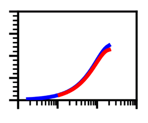
Figure 4 shows data from Wu & Moin (Reference Wu and Moin2008) (see their figures 1 and 9) at $Re = 5300$ and $Re = 44\,000$ (dashed lines), and (4.7) for the same values of $Re$ (solid lines) taking the shear-layer limiting value as ${{\mathcal {R}}}_c = 250$. These correspond to $M$ values of $2.5 \times 10^{2}$, $1.6 \times 10^{3}$ and $\hat {d}$ values of $1.2 \times 10^{-1}$, $2.0 \times 10^{-2}$, respectively, so that $M \hat {d} \approx 32$. The chosen value of ${{\mathcal {R}}}_c$ thus implies a depth of the wall layer of approximately 23 wall units, i.e. $M \hat {d} / \sqrt {2} \approx 23$, see (2.13). This is smaller, though of comparable magnitude to the usual estimate of around 30 wall units.

Figure 4. Mean flow speed in the wall layer. The solid lines show predictions for $Re = 5300$ (blue) and $Re = 44\,000$ (red) using equation (4.7) over the range $10^{-3}<\hat {y}<\hat {d}$. The dashed lines show loci of data from Wu & Moin (Reference Wu and Moin2008) at the same values of $Re$, also in blue and red, respectively. The inset shows the same data at low values of $\hat {y}$, with both axes logarithmic.

With this value of ${{\mathcal {R}}}_c$, it can be seen that (4.7) matches closely to the data over a large part of the wall-layer range, although there is a deviation from the data at the inner end of the wall layer (noting that the ordinate of the main plot in figure 4 is linear).

It may be expected that a more sophisticated model of ${{\mathcal {L}}}$ and/or $G$ could improve the model here. Smoothing the transition from the wall layer to the core may also improve the small underestimate of the wall-layer depth.

At the greater $Re$ value, the maximum speed from this model corresponds closely to the approximation (4.5).