3.1. Axisymmetric problem and co-moving frame

In the following, we will focus on the axial self-propulsion of the particle, for which the problem remains completely axisymmetric. In steady state, the concentration and velocity fields are time independent when measured in a reference frame moving with the particle. For convenience (e.g. to avoid any need for remeshing of the computational domain), we analyse the problem in that co-moving reference frame, where the particle is fixed, and the boundary conditions for the velocity field become

(3.1a,b)\begin{equation} \left. \boldsymbol{u}\right|_{\varGamma_p} = \boldsymbol{\tilde{u}},\quad \left. \boldsymbol{u}\right|_{{\varGamma_d}} ={-}U_z {\boldsymbol{e}_z}, \end{equation}

where $U_z$ is the physical velocity of the particle relative to the wall in the laboratory frame, and completely determines the steady self-propulsion dynamics of the particle along the confining tube's axis (see figure 1).

Figure 1. Self-propulsion of a single isotropic phoretic particle of radius $a$ along the axis of a cylindrical pipe of radius $R$ (viewed here in the reference frame of the particle). The particle-to-pipe radius ratio, $\kappa =a/R$, is a measure of the level of confinement. The particle and pipe surfaces are noted $\varGamma _p$ and $\varGamma _d$, respectively. Here $\varGamma _{in}$ and $\varGamma _{out}$ denote cross-sections of the pipe far ahead and behind the particle, respectively. Inset: within a thin interaction layer of thickness $\lambda$, local surface gradients in the chemical solute (orange) released from the particle surface induce a net hydrodynamic slip.

It should be noted nevertheless that the numerical methodology presented in the following can be generalised to non-axisymmetric and unsteady configurations. Unsteady simulations of the particle's dynamics in the laboratory frame were also performed with non-axisymmetric initial conditions (i.e. particle position, direction and intensity of the particle velocity) and showed that this axisymmetric self-propulsion state is a stable attractor for the problem when ${Pe}<15$, for all $\kappa$: when the particle is released initially away from the axis, it relaxes after a transient to either a stationary state on the axis or steady propulsion along the axis, establishing the physical relevance of the axisymmetric setting considered here.

3.2. Numerical method

Equations (2.3a,b), (2.4) and (2.7a,b), with boundary conditions, (2.5a,b) and (3.1a,b), form a fully coupled set of nonlinear partial differential equations problem. We solve these equations numerically in a cylindrical domain of length $L\gg R$ with the particle located at its centre.

Boundary conditions must be prescribed for the solute and flow fields on the upstream and downstream cross-sections of the computational domain, $\varGamma _{in}$ and $\varGamma _{out}$ located respectively at $z=\pm L/2$ from the centre of the particle. In the lab frame, the fluid is expected to be at rest with a homogeneous concentration of solute, far enough upstream and downstream of the particle, so that, in the reference frame co-moving with the particle,

(3.2a,b)\begin{equation} \left.\boldsymbol{u}\right|_{\varGamma_{in},\varGamma_{out}}={-}U_z\boldsymbol{e}_z,\quad \left.\frac{\partial c}{\partial z}\right|_{\varGamma_{in},\varGamma_{out}}=0, \end{equation}

with $U_z$ the a priori unknown particle velocity, which is determined as part of the solution by enforcing the force-free condition on the particle.

As for the inertial fluid–solid coupling in high Reynolds configurations (Selçuk et al. Reference Selçuk, Ghigo, Popinet and Wachs2021), the presence of the nonlinear advective coupling in the solute transport equations prevents the use of other popular numerical techniques such as multipole expansion (Sangani & Mo Reference Sangani and Mo1996), boundary elements methods (Pozrikidis Reference Pozrikidis1992; Montenegro-Johnson et al. Reference Montenegro-Johnson, Michelin and Lauga2015) or the force coupling method (Delmotte et al. Reference Delmotte, Keaveny, Plouraboué and Climent2015; Rojas-Pérez et al. Reference Rojas-Pérez, Delmotte and Michelin2021), which are particularly suitable for purely diffusive problems. In such a limit, a detailed knowledge of the flow and concentration fields in the domain bulk (i.e. away from the computational domain boundary $\varGamma =\varGamma _p\cup {\varGamma _d}\cup \varGamma _{in}\cup \varGamma _{out}$) is unnecessary to obtain the particle dynamics. In contrast, when ${Pe}\neq 0$, the presence of the advective contribution to the solute transport, $\boldsymbol {u} \boldsymbol {\cdot }\boldsymbol {\nabla } c$, which is key to the understanding and capture of the spontaneous self-propulsion of isotropic phoretic particles and droplets (Michelin et al. Reference Michelin, Lauga and Bartolo2013; Izri et al. Reference Izri, van der Linden, Michelin and Dauchot2014), imposes a change in the resolution paradigm, by requiring to determine $\boldsymbol {u}$ and $c$ everywhere in the computational domain, and an accurate numerical treatment of this nonlinear term in the solute transport equation.

We present here a novel approach to solve for the diffusiophoretic propulsion based on Basilisk, a popular open source framework for computational fluid dynamics (Popinet Reference Popinet2015). Borrowing techniques developed for high-${Re}$ flow simulations, the nonlinear diffusiophoretic problem is split into multiple sub-problems. The equations of evolution for the solute and flow fields are solved using finite volumes on hierarchically arranged, adaptive quadtree/octree grids (Popinet Reference Popinet2003). To adapt to the Basilisk framework most efficiently, the hydrodynamic problem is described by the unsteady Stokes equations with a small Reynolds number (${Re}=0.05$). To reach the steady-state solutions, the hydrodynamic solver is called iteratively on a pseudo-time $\tilde {t}$, until the residuals between two pseudo-time steps reaches a convenient threshold, i.e. ${| \boldsymbol {u}(\tilde {t}+{\rm \Delta} \tilde {t}) - \boldsymbol {u}(\tilde {t}) | \lesssim 10^{-6} | \boldsymbol {u}(\tilde {t}) | }$, which generally takes $\mathcal {O}(10)$ successive calls. Note that this step represents the most time consuming part of the method. Stokes equations are solved using an operator-splitting method (Bell, Colella & Glaz Reference Bell, Colella and Glaz1989), with a viscous step (Poisson solver) followed by a projection onto a divergence-free space (Helmholtz solver). For the solute transport, (2.4), the diffusive Laplacian term is handled implicitly while the advective contribution is computed using the Bell–Colella–Glaz second-order upwind method (Bell et al. Reference Bell, Colella and Glaz1989).

The description of all solid–fluid interfaces that do not match a rectangular mesh is based on the method of embedded boundaries (Johansen & Colella Reference Johansen and Colella1998; Schwartz et al. Reference Schwartz, Barad, Colella and Ligocki2006), allowing for a second-order accurate computation of the additional fluxes to be included in the finite-volume balance in order to enforce a prescribed boundary condition within cells containing a fluid–solid interface $\varGamma _p$ or ${\varGamma _d}$ (Schneiders et al. Reference Schneiders, Günther, Meinke and Schröder2016). Hydrodynamic forces are then computed a posteriori by numerical integration of the stress tensor on the particle surface.

At this point, we dispose of an efficient numerical framework for the computation of the flow velocity and solute concentration, $(\boldsymbol {u},p, c)$, for boundaries of any shape, for a given particle velocity. The dynamics of the particle (here completely characterised by $U_z$, its axial velocity) is further determined through the instantaneous force-free constraint, which writes here simply as $F_z=0$. The Stokes problem is linear regardless of the confinement level $\kappa$; therefore, the axial force on the particle is an affine function of the solid body translation $U_z$, for a given slip velocity $\tilde{\boldsymbol{u}}$, i.e.

(3.3)\begin{equation} F_z(\boldsymbol{\tilde{u}},U_z) = \mathcal{R} U_z + \mathcal{Q}(\tilde{\boldsymbol{u}}), \end{equation}

with $\mathcal {R}$ is the axial drag coefficient on a rigid sphere translating along the axis of the cylindrical pipe and $\mathcal {Q}$ is a scalar that is completely determined by the surface slip and the level of confinement. Both $\mathcal {Q}$ and $\mathcal {R}$ are independent of $U_z$ and solely depend on geometry (and on the slip velocity in the case of $\mathcal {Q}$), and are determined numerically as follows. At each time step, the Stokes problem is solved twice for the same slip velocity $\tilde {\boldsymbol {u}}$: (i) for the real problem, using a first guess of the swimming speed $U_z$ from the previous time step, and (ii) for an auxiliary problem with a different and arbitrary $U_z^{aux}$. For each, the corresponding axial force on the particle is computed and, using both solutions together with (3.3), provides $(\mathcal {Q},\mathcal {R})$ from which the correct swimming speed satisfying the force-free condition is obtained as $U_z(F_z=0)=-\mathcal {Q}/\mathcal {R}$.

A cubic domain of size $L/a=128$ was used on an adaptive mesh refinement, with the finest spatial discretisation reaching $32$ computational cells per particle radius $a$, with ${\approx }2000$ cells describing the particle surface. The fluid domain (figure 1) is then cut out from this cubic volume employing the embedded boundaries approach (Bell et al. Reference Bell, Colella and Glaz1989) and the particle is set in the origin of the coordinate system, placed in the centre of the computational cuboid. Mesh is automatically adapted so as to ensure that maximum spatial refinement is always ensured on top of solid–liquid interfaces. Elsewhere, mesh is refined (respectively coarsened) whenever velocity or solute gradients is more (respectively less) than a prescribed threshold using an adaptive wavelet algorithm (see, e.g. van Hooft et al. Reference van Hooft, Popinet, van Heerwaarden, van der Linden, de Roode and van de Wiel2018). Using this approach and comparing the results for maximum spatial discretisations of 32 and 64 cells per unit length, we obtained a match in both swimming velocity and solute concentration fields, with a typical discrepancy on the swimming velocity lower than 0.1 % (${Pe}=6$, $\kappa =0.5$) and reaching a maximum $2\,\%$ discrepancy for the most confined case considered (${Pe}=6$, $\kappa =0.9$).

3.3. Validation

We now proceed with the validation of the proposed framework and algorithms by testing the main physical features against classical literature cases, namely (i) the self-propulsion of a model micro-organism using a prescribed surface slip (i.e. a so-called squirmer) in strong spatial confinement (Zhu et al. Reference Zhu, Lauga and Brandt2013), and (ii) the self-propulsion of isotropic particles due to nonlinear hydrochemical coupling (Michelin et al. Reference Michelin, Lauga and Bartolo2013). The first case, for which the hydrodynamic slip is imposed, allows for the validation of the hydrodynamic solver and the enforcement of the force-free constraint, while the second provides a validation of the coupled hydrochemical solver.

3.3.1. Squirmer in a pipe

The behaviour of a single squirmer inside a cylindrical pipe for different levels of confinement is considered, as studied in Zhu et al. (Reference Zhu, Lauga and Brandt2013) using a boundary element method. A steady slip velocity $\tilde {\boldsymbol{u}}$ is imposed on the particle surface, which corresponds to a neutral squirmer, which would swim at a velocity $U_z^*\boldsymbol {e}_z$ in the absence of any confinement, namely

(3.4)\begin{equation} \tilde{\boldsymbol{u}}^{squirmer}={-}\frac{2U_z^{*}}{3} (\boldsymbol{I}-\boldsymbol{n}\boldsymbol{n})\boldsymbol{\cdot}\boldsymbol{e}_z. \end{equation}

For an unconfined case, the algorithm recovers within ${\pm }0.1\,\%$ the swimming velocity predicted by the reciprocal theorem (Stone & Samuel Reference Stone and Samuel1996), i.e. the average of the surface slip velocity (3.4) on the particle surface. For confined cases, with $0<\kappa \leq 0.5$, the maximum relative error between the present results and that of Zhu et al. (Reference Zhu, Lauga and Brandt2013) is less than $2\,\%$ (table 1).

Table 1. Steady-state swimming speed of a squirmer along the axis of a capillary tube for varying confinement ratio $\kappa$ and comparison with the results of Zhu et al. (Reference Zhu, Lauga and Brandt2013). The swimming velocity is normalised by that in unbounded fluid domains.

Physically, for the axisymmetric configurations tested here, the squirmer's swimming velocity is observed to decrease with increasing confinement.

3.3.2. Autophoretic propulsion in an unbounded domain

The second comparison allows for the validation of the hydrochemical solver in the absence of confinement ($\kappa \ll 1$) and, in particular, of the treatment of the nonlinear advective coupling of the Stokes and chemical problems, which is the essential ingredient of the spontaneous autophoretic motion studied here. The results are then compared with those of Michelin et al. (Reference Michelin, Lauga and Bartolo2013) for strictly unbounded domains. Steady self-propulsion is observed beyond a critical ${Pe}$ after a transient, with a constant non-zero swimming speed as depicted in figure 2. A detailed comparison with the results of Michelin et al. (Reference Michelin, Lauga and Bartolo2013) shows that the present method is able to recover the correct swimming velocity with an error lower than ${\approx } 1\,\%$ for the resolution considered (table 2).

Figure 2. Unsteady axisymmetric propulsion velocity $U_z(t)$ of an isotropic phoretic particle along the capillary's axis for increasing level of confinement $\kappa$ (colour) and ${Pe}=2.5$. The results are reported for $\kappa =1/16$, $1/8$, $1/4$, $1/2$, $2/3$ and $3/4$. During the initialisation phase ($t< t_{s}$ with $t_s=25$), the slip velocity on the particle surface is imposed (neutral squirmer), (3.4); for $t>t_{s}$, the phoretic slip velocity and particle dynamics are computed based on the actual surface concentration distribution of the solute, (2.2), and the force-free condition on the particle.

Table 2. Steady-state swimming velocities as a function of ${Pe}$, for an isotropic autophoretic particle in an unbounded domain, and comparison with the results of Michelin et al. (Reference Michelin, Lauga and Bartolo2013) for infinite domains.

4.1. Unsteady vs steady-state self-propulsion

In practice, the coupled equations for the solute concentration and fluid velocity are integrated numerically in time for fixed values of the Péclet number ${Pe}$ and confinement ratio $\kappa$. For $0\leq {Pe}\leq 15$, at long time, the particle propels at a steady velocity along the capillary axis: an axisymmetric steady state is therefore reached in the reference frame of the particle for the solute concentration and flow fields, and we specifically focus here on the characterisation of such axisymmetric steady states.

The simulation is initialised by prescribing during a short initialisation phase ($0\leq t\leq t_s$ with $t_s=25$ in non-dimensional units) a fixed axisymmetric slip velocity on the surface of the particle, corresponding to a neutral squirmer with intrinsic swimming velocity $U_z^*=0.1$. For $t\geq t_s$, the true phoretic slip is computed directly from the actual concentration distribution and imposed at the particle surface. Such a procedure allows us to perturb the system and break the left-right symmetry. The resulting evolution of the swimming velocity is shown in figure 2 for ${Pe}=2.5$ and for an increasing level of confinement. The self-propulsion of the particle during the initialisation (squirmer) phase decreases with $\kappa$, in agreement with the results of Zhu et al. (Reference Zhu, Lauga and Brandt2013); indeed, in figure 2 the velocity $U_z$ in the initialisation phase ($t\leq 25$) where the slip velocity is imposed, is observed to be lower for larger values of $\kappa$ (tighter confinement).

For $t\geq t_{s}$, once the actual phoretic slip condition is enforced, the particle relaxes after a transient toward its steady-state dynamics. Unless indicated otherwise, we thus refer to $U_z$ as the steady-state self-propulsion velocity of the particle when $t\gg t_s$. Two fundamentally different types of steady-state dynamics are observed in figure 2 for ${Pe}=2.5$, depending on the level of lateral confinement $\kappa$ of the particle. For weak confinement (i.e. small $\kappa$), the particle slows down and eventually comes to a stop; this is consistent with ${Pe}=2.5$ being lower than the critical threshold for self-propulsion in unbounded domains (${Pe}_c=4$ for $\kappa =0$) (Michelin et al. Reference Michelin, Lauga and Bartolo2013). Note that a steady state is reached for the particle velocity, flow field and concentration gradients, but not the average concentration which keeps increasing in time due to the fixed emission of solute at the particle surface and the confinement of the particle by chemically inert walls. In contrast, for $\kappa \geq 0.2$, the particle maintains a net velocity that increases with $\kappa$ and saturates for the strongest confinements considered ($\kappa \approx 0.8$). Note that changing the magnitude of the initialisation velocity or the duration of the initialisation phase only modified the transient regime past $t\geq t_s$, but did not alter the nature of the observed steady state (i.e. fixed or self-propelled particle).

4.2. Self-propulsion velocity and critical threshold

In the following, we focus on the evolution of this steady-state self-propulsion and the influence of the proximity of the confining walls. To that end, for ${0\leq \kappa \leq 0.8}$ and ${0<{Pe}\leq 15}$, we systematically run time-dependent simulations until a steady state is reached, with a constant swimming speed along the axis of the capillary. The results for $U_z({Pe},\kappa )$ are reported in figure 3, and demonstrate the strong influence of confinement and an increase of the self-propulsion velocity with confinement $\kappa$ for all ${Pe}$. This effect is significant provided the distance to the wall is of the order of a few particle radii ($\kappa \gtrsim 0.2$), confirming experimental observations (de Blois et al. Reference de Blois, Bertin, Suda, Ichikawa, Reyssat and Dauchot2021).

Figure 3. (a) Steady-state axisymmetric swimming velocity $U_z$ of an isotropic active particle as a function of the convection-to-diffusion ratio, ${Pe}$, and for increasing confinement $\kappa$ (colour). (b) Same as (a) in logarithmic scale. The results for a single isolated particle in unbounded domains ($\kappa =0$, Michelin et al. Reference Michelin, Lauga and Bartolo2013) is shown for comparison (red dashed line). In (b) the dotted black line indicates the minimum velocity to determine the emergence of a net propulsion. The results are reported here for $\kappa =1/16$, $1/8$, $1/4$, $3/8$, $1/2$, $2/3$ and $3/4$.

Beyond a systematic increase of the swimming velocity, figure 3 also demonstrates several other important features. Most importantly, confinement effects are strongest for low-to-moderate values of ${Pe}$. We first note a significant reduction with $\kappa$ of the critical self-propulsion threshold ${Pe}_c$. Furthermore, the presence of confinement strongly affects the evolution of $U_z({Pe})$: in weakly confined configurations the velocity varies non-monotonically with $\mbox {Pe}$, and increases smoothly from the threshold until it saturates for ${Pe}\approx 10$–$20$ and decreases as ${Pe}$ is increased further (Michelin et al. Reference Michelin, Lauga and Bartolo2013). In contrast, the velocity of strongly confined particles ($\kappa \gtrsim 0.5$) scales as $1/\sqrt {{Pe}}$ for most of the parameter range except in the immediate vicinity of the threshold ${Pe}_c(\kappa )$ where it increases sharply with ${Pe}$ (figure 3b). As a result, the maximum swimming velocities are observed at low Péclet in strongly confined environments (figure 3a). Note that self-sustained motion is never observed for ${Pe}=0$, regardless of $\kappa$: as for unbounded environments, convective transport of the solute by the phoretic flows is essential to the propulsion of isotropic particles, as it provides the required symmetry-breaking mechanism (Michelin et al. Reference Michelin, Lauga and Bartolo2013; Izri et al. Reference Izri, van der Linden, Michelin and Dauchot2014).

Stronger confinement significantly promotes self-propulsion, by reducing the minimum Péclet number, ${Pe}_c$ required for self-sustained autophoretic motion: while ${Pe}_{c}=4$ for $\kappa =0$, the existence of a minimum ${Pe}$ for self-propulsion persists throughout the range of confinement investigated but this threshold drops quickly as $\kappa$ is increased, with ${Pe}_c\approx 0.1$ for $\kappa \gtrsim 0.5$ (figure 4). However, with the present numerical approach, it is not possible to analyse the lubrication limit with significant precision to conclude on the asymptotic behaviour of ${Pe}_c$ when $1-\kappa \ll 1$, and this asymptotic limit would require further analysis using a different approach.

Figure 4. (a) Evolution with confinement ($\kappa$) of the critical threshold ${Pe}_c$ for the onset of propulsion. For fixed $\kappa$, the numerical uncertainties on ${Pe}_c$ are defined using the smallest (respectively largest) value of ${Pe}$ for which the steady-state velocity is greater (respectively smaller) than a numerical threshold $U_z^*=5\times 10^{-3}$. (b) Evolution of the rescaled particle velocity with confinement $\kappa$.

Except for rare examples (Hokmabad et al. Reference Hokmabad, Dey, Jalaal, Mohanty, Almukambetova, Baldwin, Lohse and Maass2021), the Péclet number is fixed in most experimental systems, and only spatial confinement can be controlled. For this reason, we also report in figure 4(b) the evolution of the rescaled swimming velocity for fixed ${Pe}$ and variable confinement $\kappa$. In all cases, this rescaled representation (where we account for the dominant ${Pe}^{-1/2}$ scaling of the velocity, see also § 5) demonstrates a non-monotonic evolution of the swimming velocity with $\kappa$, with a maximum at $\kappa \approx 2/3$, before entering the lubrication regime. This behaviour and its origin will be further discussed in § 5.1.

4.3. Effect of confinement on the solute distribution

The peculiar evolution of the swimming velocity with confinement and its enhancement at low ${Pe}$ is analysed by considering the detailed variations of the solute concentration around the isotropic phoretic particle in confined steady-state regimes (figure 5). For fixed ${Pe}$, the solute distribution around the particle is fundamentally modified by confinement.

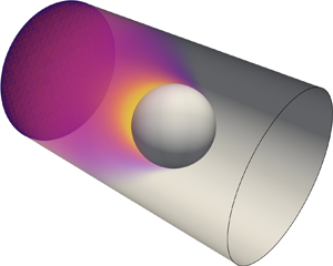
Figure 5. Steady-state relative solute concentration distribution and representative streamlines (colour coded by the fluid velocity magnitude) around an isotropic phoretic particle in axisymmetric confinement for ${Pe}=6$ and increasing $\kappa$ (in the laboratory reference frame, i.e. fixed with respect to the capillary walls).

In unbounded domains and for weak confinements, the solute distribution is characterised by a monotonic decrease in all radial directions around the particle, with a small front-back asymmetry maintained by the self-generated phoretic flows (figure 5, $\kappa =0.1$): in that case, the solute production at the particle surface is predominantly balanced by its radial diffusion away from the particle.

In contrast, for stronger levels of confinement (e.g. figure 5, $\kappa =0.8$), lateral diffusion of the solute away from the particle is prevented by the lateral inert wall ${\varGamma _d}$: in that case, the solute production by the particle's catalytic surface is predominantly balanced by its downstream convective transport by the phoretic flows. As a result, the capillary upstream from the particle is essentially solute free, and the solute concentration saturates downstream from the particle at a much larger and uniform value. The largest solute concentrations are therefore found downstream and away from the particle, rather than on its surface as for the unbounded configuration.

A more detailed observation for strong confinement reveals that far upstream and downstream from the particle, the solute concentration becomes homogeneous due to the rapid lateral diffusion across the capillary (figure 5, $\kappa =0.8$). Additionally, as confinement is increased, the fluid layer separating the particle from the wall becomes very thin and chemical diffusion across this thin gap becomes dominant over other solute transport mechanisms: as a result, the solute concentration is homogenised across the whole fluid layer, despite the steady emission of solute from the particle surface (figure 5, $\kappa =0.8$, zoom).

This last observation is further confirmed quantitatively by the detailed evolution of the distribution of the concentration across the thin fluid layer (figure 6a). While the solute concentration is only significant near the surface of the particle for small $\kappa$, the distribution of solute across the gap is uniform when $\kappa \rightarrow 1$.

Figure 6. Relative spanwise distribution of (a) solute concentration and (b) streamwise flow velocity (in the particle's reference frame) within the fluid gap between the swimmer and the fixed walls ($z=0$) for increasing confinement $\kappa$ (colour) and ${Pe} = 6.0$. The rescaled radial variable $\hat {r}=(r-a)/(R-a)$ is defined such that $\hat {r}=0$ (respectively $\hat {r}=1$) corresponds to the particle (respectively wall) surface for all values of $\kappa$. In (b) the rescaled fluid velocity with respect to the particle is $\hat {w}=(w+U_z)/(w_{slip}+U_z)$ (note: here $w<0$ throughout the gap in the particle reference frame, and $w=-U_z$ at the wall, $\hat {r}=1$, while $w=w_{slip}<0$ at the particle surface, $\hat {r}=0$). The results are reported for $\kappa =n/10$ with $1\leq n\leq 9$.

The dominance of lateral diffusion, and resulting homogenisation of the concentration in most of the domain (i.e. apart from $|z|\sim 1$), justifies focusing on the mean concentration along the capillary axis, defined as the average within each cross-section (fixed $z$),

(4.1)\begin{equation} \langle c\rangle _{xy}(z)=\frac{1}{{\rm \pi} (R^2-R_{min}(z)^2)} \int_{R_{min}(z)}^R\int_0^{2{\rm \pi}}c(r,z)r\,\mathrm{d} r\,\mathrm{d} \theta, \end{equation}

with $R_{min}(z)=\sqrt {a^2-z^2}$ for $|z|< a$ and $R_{min}(z)=0$ otherwise. This function of $z$ only takes a uniform value far upstream and downstream of the particle (figure 7), so that the front-back concentration contrast can be defined as

(4.2)\begin{equation} {\rm \Delta} c=\langle c\rangle _{xy}(z={-}L/2)-\langle c\rangle _{xy}(z=L/2). \end{equation}

Figure 7(a) shows that the evolution with $z$ of the average concentration, once rescaled by ${\rm \Delta} c$, becomes essentially independent of $\kappa$ for $\kappa \gtrsim 0.5$, and that this universal profile is characterised by (i) constant values behind and ahead of the particle ($z<-1$ or $z\gtrsim 2$) and (ii) a linear profile (constant streamwise gradient) in most of the vicinity of the particle. The amplitude of the front-back concentration contrast however increases sharply with $\kappa$, diverging as $(1-\kappa )^{-1/2}$ as $\kappa \rightarrow 1$, demonstrating the confinement-induced chemical saturation (figure 7b). This behaviour is quantitatively consistent with the asymptotic predictions (5.26) (see also § 5).

Figure 7. (a) Evolution of the spanwise-averaged solute concentration in the fluid around the particle along the pipe for increasing confinement $\kappa$ (colour) for ${Pe}=6$. The particle's position and limits are shown (respectively dash-dotted and dotted lines). The results are reported for $\kappa =n/10$ with $2\leq n\leq 8$. (b) Evolution with $\kappa$ of the front-back concentration contrast measured using the spanwise-averaged concentration at $|z|\gg R$ upstream and downstream from the particle. The dashed line corresponds to the analytical prediction of § 5; see (5.26a–c).

The fore-aft asymmetry of the concentration profile, observed in figure 7(a) for ${Pe}=6$, results from the accumulation of solute in the wake of the propelling droplet due to the restricted lateral diffusion when the droplet is sufficiently confined (large enough $\kappa$) and is also present for larger ${Pe}$. A small overshoot of the concentration profile can be observed immediately behind the particle for the least confined configurations (small $\kappa$) for which the solute transport balance is fundamentally different.

4.4. Effect of confinement on the flow field

The flow pattern and intensity generated by the swimming particle inside the capillary is also significantly modified by the presence and distance to the neighbouring walls. For strong confinement, the largest fluid velocities and velocity gradients are observed within the thin fluid gap: a finite volume of fluid needs to be moved from one side of the particle to the other through a narrower gap in order to allow for the particle motion through the capillary where the flow is at rest away from the particle. As $\kappa$ approaches $1$, the typical fluid velocity within the gap is therefore much higher than the particle velocity itself (see also § 5 for a more quantitative discussion), resulting in strong spanwise gradients of the fluid streamwise velocity within the narrow gap (figure 5).

A more detailed analysis of the velocity distribution within the fluid gap further reveals that, as $\kappa$ is increased, the velocity profile tends to a Couette flow profile (figure 6b): the dominant fluid transport in the narrowest fluid layer is therefore driven solely by the phoretic slip at the particle surface, resulting from the front-back concentration contrast observed in strongly confined configurations (figure 5). In particular, the absence of curvature in the velocity profile indicates that longitudinal pressure gradients play a negligible effect on the dominant flow.

We therefore turn our attention to the evolution of this slip forcing for increasing $\kappa$ and, more specifically, on its streamwise component that plays a major role in the thinnest regions. Once again, a transition can be clearly seen between two different regimes (figure 8a): for weak confinement, the relative distribution of slip is rather constant along the sphere, except near the front and back poles. A slight maximum is observed at the back of the particle, which is in qualitative agreement with the established result that the particle acts as a pusher swimmer in unbounded domains (Michelin et al. Reference Michelin, Lauga and Bartolo2013; Izri et al. Reference Izri, van der Linden, Michelin and Dauchot2014). As confinement is increased, the slip profile becomes more front-back symmetric with a maximum value attained in the narrowest region: this indicates a stronger localisation of the forcing in the regions where it has the most hydrodynamic influence on the self-propulsion. Note that such localisation in the regions of strongest hydrodynamic influence was also recently identified for a chemically active droplet propelling along a planar wall (Desaï & Michelin Reference Desaï and Michelin2021). The evolution of the maximum phoretic slip with $\kappa$ confirms the enhancement of the phoretic forcing as the distance to the confining walls is reduced, with the average fluid velocity in the gap, $W=\langle w(z=0)\rangle _{xy}$, diverging as $(1-\kappa )^{-1}$ when $\kappa \rightarrow 1$. This increase of the phoretic slip with confinement directly results from the increased (and diverging as $\kappa \rightarrow 1$) concentration contrast between the front and back of the phoretic particles that was discussed in greater details in § 4.3. The results are in good agreement with the asymptotic prediction for the evolution of $W$ as $\kappa \rightarrow 1$ (figure 8(b) and (5.26a–c)).

Figure 8 (a) Distribution of the surface slip velocity normalised by the average fluid velocity in the particle-capillary gap. The results are reported for $\kappa =n/10$ with $2\leq n\leq 8$. (b) Average fluid velocity in the particle-capillary gap $W$ at varying confinement $\kappa$. Results are shown here for ${Pe}=6.0$. The dashed line corresponds to the analytical prediction, (5.26a–c).

Finally, the velocity field away from the particle (i.e. upstream and downstream) is almost uniform and eventually decays to zero (in the laboratory reference frame). Here a brief comment should be made regarding the boundary conditions imposed at the inlet and outlet boundaries of the computational domain (figure 1). A Dirichlet boundary condition on the flow velocity is imposed on $\varGamma _{in}$ and $\varGamma _{out}$, representing that the flow is at rest far upstream and downstream from the particle in the lab frame. This will be the case, for example, when the domain considered (figure 1) is part of an infinitely long tube: away from the particle, the large hydrodynamic resistance prevents the existence of any flow within the tube.

4.5. Resistance to particle motion and pressure

We noted earlier that, because fluid is at rest in front of and behind the phoretic particle, a finite volume of fluid must pass through the thin fluid gap for the particle to move forward. Driving such a volume flux through a thin viscous fluid layer results in the establishment of a net pressure difference between the front and back of the sphere, as demonstrated in figure 9 by the evolution of the spanwise-averaged pressure $\langle p \rangle _{xy}$ along the capillary (i.e. its average on each cross-section) and of the front-back pressure difference ${\rm \Delta} p$ (both quantities defined in a similar way as their counterparts for the concentration).

Figure 9. (a) Evolution of the spanwise-averaged fluid pressure in the fluid around the particle for increasing confinement $\kappa$ (colour). The particle's position and limits are shown (respectively dash-dotted and dotted lines). The results are reported for $\kappa =n/10$ with $1\leq n\leq 9$. (b) Evolution with $\kappa$ of the front-back mean pressure difference measured using the spanwise-averaged pressure at $|z|\gg R$ upstream and downstream from the particle. In both panels, results were obtained for ${Pe}=6$. The dashed line with $(1-\kappa )^{-3/2}$ is shown for comparison only.

We first note that the pressure difference ${\rm \Delta} p$ vanishes when $\kappa \ll 1$, i.e. for unbounded phoretic particles, as expected. When $\kappa$ becomes larger, the pressure still reaches constant values far upstream and downstream of the particle, but they are now different and their difference quickly grows with confinement and diverges as $\kappa \rightarrow 1$ (figure 9b). While a clear scaling is difficult to identify from the numerical results, it can still be concluded that the divergence observed is weaker than $(1-\kappa )^{-2}$ (see § 5.2 for further discussion). The emergence of a finite (and increasing) pressure difference exerts a resisting force on the particle, balancing the net forcing exerted within the thin fluid gap by the phoretic flows generated by the particle.

It should further be noted that the pressure variations are not monotonic, showing a local minimum in the vicinity of the narrowest regions (figure 9a).

5.1. Global conservation arguments

The analyses and results of the previous sections provide some critical insight on the physical balances and phenomena determining the evolution of the confined self-propulsion, in particular in the limit of strong confinement ($\kappa \gtrsim 0.5$).

In the following, these different arguments are summarised and combined to obtain a prediction for the scaling of the swimming velocity in this limit, in terms of the two main parameters of the problem, ${Pe}$ and $\kappa$. Throughout, we focus exclusively on the steady-state regime at the centre of our attention in § 4. We will relate three specific quantities: (i) $U_z$ the swimming velocity of the phoretic particles, (ii) ${\rm \Delta} c$ the difference in the uniform solute concentration observed far downstream and upstream of the particle, respectively, and (iii) $W=\langle w(z=0)\rangle _{xy}$ the mean flow velocity (relative to the particle) through the narrowest fluid region ($z=0$) (oriented along $-\boldsymbol {e}_z$, i.e. from the front toward the back).

5.1.1. Solute conservation

Considering the entire computational domain as a control volume, the conservation of solute imposes

(5.1)\begin{equation} \int_{\varGamma}\boldsymbol{j}\boldsymbol{\cdot} \boldsymbol{n}\,\mathrm{d} S=0, \end{equation}

with $\varGamma =\varGamma _p\cup \varGamma _d\cup \varGamma _{out}\cup \varGamma _{in}$ (figure 1), $\boldsymbol {n}$ the unit normal to $\varGamma$ pointing into the fluid domain, and $\boldsymbol {u}$ the fluid velocity in the reference frame of the particle. The non-dimensional solute flux $\boldsymbol {j}={Pe} c\boldsymbol {u}-\boldsymbol {\nabla } c$ (characteristic scale: $|\mathcal {A}|$) includes the contributions of convective transport by the fluid flow and diffusion, respectively.

The channel's wall are inactive and impermeable so that $\boldsymbol {j}\boldsymbol {\cdot }\boldsymbol {n}=0$ on $\varGamma _d$. At the particle surface the solute flux is purely diffusive and matches the total production rate at the particle surface $\int _{\varGamma _p}\boldsymbol {j}\boldsymbol {\cdot }\boldsymbol {n}\,\mathrm {d} S={4{\rm \pi} }$. Far from the particle, near $\varGamma _{in}$ and $\varGamma _{out}$, the concentration is uniform so that the diffusive flux is negligible on these surfaces. The velocity is also uniform and equal to $-U_z\boldsymbol {e}_z$ so that

(5.2)\begin{equation} \int_{\varGamma_{in}\cup\varGamma_{out}}\boldsymbol{j}\boldsymbol{\cdot}\boldsymbol{n}\,\mathrm{d} S={-} \frac{{\rm \pi} {{Pe}\,}U_z{\rm \Delta} c}{\kappa^2}. \end{equation}

Equation (5.1) then leads to

(5.3)\begin{equation} {Pe} \,U_z{\rm \Delta} c=4\kappa^2. \end{equation}

This result was found in agreement with the numerical results for strong enough confinements ($\kappa \gtrsim 0.2$, figure 10). Note that for lower $\kappa$, such a balance is not expected to hold as the transport mechanism of the solute away from the particle surface vicinity is fundamentally different.

Figure 10. Global conservation of solute: the dimensionless solute emission ($\kappa ^2$) is compared with the dimensionless excess solute convected downstream from the sphere (${Pe}\,U_z{\rm \Delta} c$).

5.1.2. Conservation of mass

A similar argument for the conservation of mass on the upstream half of the computational domain leads to

(5.4)\begin{equation} \int_{\varGamma^+}\boldsymbol{u}\boldsymbol{\cdot}\boldsymbol{n}\,\mathrm{d} S=0, \end{equation}

with $\varGamma ^+=\varGamma _{in}\cup \varGamma _p^+\cup \varGamma _d^+\cup \varGamma _0$ with $\varGamma _d^+$ and $\varGamma _p^+$ the parts of the wall and particle surfaces with $z>0$, and $\varGamma _0$ the fluid cross-section at $z=0$. The particle surface $\varGamma _p$ and the wall $\varGamma _d$ are impermeable and do not contribute to the integral above. On $\varGamma _{in}$, the velocity is uniform and equal to $-U_z$, so that $\int _{\varGamma _{in}}\boldsymbol {u}\boldsymbol {\cdot }\boldsymbol {n}\,\mathrm {d} S={\rm \pi} U_z/\kappa ^2$. By definition of $W$, $\int _{\varGamma _0}\boldsymbol {u}\boldsymbol {\cdot }\boldsymbol {n}\,\mathrm {d} S=-{\rm \pi} (1-\kappa ^2)W/\kappa ^2$, so that

(5.5)\begin{equation} U_z=(1-\kappa^2)W. \end{equation}

5.1.3. Fluid velocity trough the gap

One of the main features of the flow within the thin fluid gap identified in § 4.2 when the gap thickness is reduced (i.e. $1-\kappa \ll 1$) was the emergence of a Couette-like dominant flow driven by the slip velocity $w_{slip}$ at the surface of the particle. For a cylindrical Couette flow (Leal Reference Leal2007),

(5.6)\begin{equation} W=\frac{w_{slip}}{2}f(\kappa),\quad \textrm{with }f(\kappa)=\frac{1}{\log(1/\kappa)}- \frac{2\kappa^2}{1-\kappa^2} \end{equation}

and $f(\kappa \rightarrow 1)=1$ (plane Couette flow). The non-dimensional slip velocity is $({\mathrm {d}c}/{\mathrm {d}z})(z=0)\approx ({\mathrm {d}}/{\mathrm {d}z})\langle c\rangle _{xy}$ since the concentration is uniform across the fluid gap for large enough $\kappa$. The results of figure 7 suggest that the variations of $\langle c\rangle _{xy}$ with $z$ are almost linear so that the axial concentration gradient in the gap is proportional to the front-back concentration contrast ${\rm \Delta} c$ and, accordingly, the phoretic slip and mean flow in the gap $W$ satisfy

(5.7)\begin{equation} W\approx K{\rm \Delta} c\end{equation}

with $K$ a constant of proportionality.

Figure 11 provides supporting evidence of this linear relationship between the average velocity $W$ and the front-back concentration contrast, with ${K\approx 1/3}$, except for the lowest ${Pe}$-values.

Figure 11. Relative evolution of the spanwise-averaged axial velocity $W$ of the fluid (relative to the particle) at $z=0$ (narrowest fluid gap) and of the front-back solute concentration ${\rm \Delta} c$. The dotted line corresponds to ${\rm \Delta} c/3$.

5.1.4. Approximation of the particle velocity

A combination of macroscopic conservation principles, (5.3) and (5.5), and qualitative argument, (5.7), allowed us to obtain three independent relationships between the three quantities of interest $U_z$, $W$ and ${\rm \Delta} c$. Combining these provide the following predictions for each of these quantities:

(5.8a–c)\begin{equation} U_z\approx 2\kappa\sqrt{\frac{1-\kappa^2}{3{Pe}}},\quad W\approx \frac{2\kappa}{\sqrt{3{Pe}(1-\kappa^2)}},\quad {\rm \Delta} c \approx 2\kappa\sqrt{\frac{3}{{Pe}(1-\kappa^2)}}. \end{equation}

These predictions are in quantitative agreements with the numerical results (figure 12) in particular for larger $\kappa$ (i.e. $\kappa \gtrsim 0.5$ or $1-\kappa ^2\lesssim 0.7$), except for the lowest value of ${Pe}$ investigated. This better agreement for larger ${Pe}$ was to be expected as convective transport of solute plays a dominant role in that limit.

Figure 12. (a) Evolution of the rescaled steady-state swimming velocity $U_z$ with ${Pe}$ and $\kappa$. In each plot, the dotted line corresponds to the equality of the two plotted quantities. (b) The same data are reported to identify the behaviour for $\kappa \rightarrow 1$.

Furthermore, this relationship shows that $U_z$ is not a monotonic function of $\kappa$ but instead should be maximum around $\kappa =1/\sqrt {2}\approx 0.7$ in agreement with the results of figure 4. These predictions also clearly establish that $U_z\sim 1/\sqrt {{Pe}}$, in particular for larger ${Pe}$ and larger $\kappa$, which is confirmed in figure 13. We finally observe that the numerical evolution of $W$ and ${\rm \Delta} c$ with $\kappa$ are consistent with these predictions (see figures 7 and 8).

Figure 13. Evolution of the rescaled particle velocity with ${Pe}$ for different confinement levels, $\kappa$. The dashed line corresponds to ${Pe}^{-1/2}$.

5.2. Asymptotic analysis

We focus now specifically on the lubrication limit, i.e. when $R\approx a$ or equivalently $\kappa \rightarrow 1$ and, thus, define $\varepsilon =1-\kappa \ll 1$. Note that, the result above establishes that the dominant swimming velocity is set solely by the slip forcing inside the hydrodynamic lubrication region of width $\sqrt {\varepsilon }$ around the region of smallest thickness (and not anywhere else). In turn, this requires knowing the leading-order evolution of the surface concentration in that region.

The scalings obtained from the balance arguments of the previous sections indicate that, for $\varepsilon =1-\kappa \ll 1$,

(5.9a,b)\begin{equation} U_z={O\left(\sqrt{\frac{\varepsilon}{{Pe}}}\right)}\quad\textrm{and}\quad {W,{\rm \Delta} c=O\left(\frac{1}{\sqrt{\varepsilon{Pe}}}\right)}. \end{equation}

Physically, this indicates that as the fluid layer between the particle and the wall is reduced, the velocity of the particle tends to zero while the front-back concentration difference diverges. This is not surprising as we focus here on the steady self-propulsion of the particle. In § 4.3 we noted that the confined limit of the particle self-propulsion corresponds to a fundamental change in the way the solute produced at the particle surface is evacuated: when $\kappa \rightarrow 0$ (unbounded flow), the solute is mostly diffused away in the far field and in all directions, while for $\kappa \rightarrow 1$, it must be convected downstream by the displacement of the particle, as steady diffusive solutions do not exist for these confined configurations. Lower self-propulsion velocities (e.g. due to the increase of viscous stresses at the boundary) therefore require larger concentration accumulation in the back of the self-propelled particle.

These arguments demonstrate not only a typical $O(\varepsilon ^{-1/2})$-scale for the magnitude of the concentration in the thin lubrication layer located between the particle and the wall (with respect to the reference concentration far ahead of the particle, taken as zero here), but also that this concentration contrast ${\rm \Delta} c$ is established at the scale of the size of the particle, so that the relevant scale of horizontal variations for $c$ is $O(1)$ not the classical $O(\varepsilon ^{1/2})$-length of the lubrication zone relevant for hydrodynamic lubrication problems. Within the thin fluid layer surrounding $z=0$, one must therefore expect

(5.10a,b)\begin{equation} c=O(\varepsilon^{{-}1/2}),\quad \tilde{u}\sim\frac{\partial c}{\partial x}=O(\varepsilon^{{-}1/2}), \end{equation}

where $\tilde u$ is the slip velocity forcing at the particle surface.

5.2.1. Hydrodynamic lubrication

When $\varepsilon \rightarrow 0$, the fluid's motion within the thin annular layer surrounding the particle at $z=0$ corresponds to a lubrication flow forced at the surface of the particle by the phoretic slip $\tilde {u}(z)$ along its surface. It is therefore described by the two-dimensional lubrication equations

(5.11a–c)\begin{equation} \frac{\partial p}{\partial \rho}=0,\quad \frac{\partial ^2{u_z}}{\partial \rho^2}=\frac{\partial p}{\partial z}, \quad\frac{\partial u_z}{\partial z}+ \frac{\partial u_\rho}{\partial \rho}=0, \end{equation}

with $\rho =\kappa ^{-1}-r$ the radial distance from the outer cylinder of radius $1/\kappa$ (measured inward) and $u_\rho$ the corresponding velocity component. The boundary conditions on the axial velocity are at leading order

(5.12a,b)\begin{equation} u_z(\rho=0,z)={-}U_z,\quad u_z(\rho=h(z),z)=\tilde{u}(z), \end{equation}

with $\rho =h(z)$ the equation for the surface of the particle, i.e.

(5.13)\begin{equation} h(z)=\frac{1}{\kappa}-\sqrt{1-z^2}\sim{\varepsilon} \left[1+\frac{z^2}{2\varepsilon}+O\left(\frac{z^4}{\varepsilon}\right)\right]. \end{equation}

Note that the present analysis is similar to that in Sherwood & Ghosal (Reference Sherwood and Ghosal2018) for the electrophoretic motion of a sphere inside a tightly fitting tube. The lubrication equations can be integrated to find the axial flow $u_z(z)$,

(5.14)\begin{equation} u_z(\rho,z)=\frac{\rho(\rho-h)}{2}{\dfrac{\mathrm{d} p}{\mathrm{d} z}}+\tilde{u}(z) \left(\frac{\rho}{h}\right)+U_z\left(\frac{\rho}{h}-1\right), \end{equation}

and integration across the fluid layer and around the particle provides the volume flux

(5.15)\begin{equation} q(z)=Q=2{\rm \pi}\int_0^hu_z(\rho,z)\,\mathrm{d} \rho={-}\frac{{\rm \pi} h^3}{6}{\dfrac{\mathrm{d} p}{\mathrm{d} z}}+ {\rm \pi}h\left({-}U_z+\tilde{u}(z)\right), \end{equation}

which must indeed be a constant for all $z$ in order to conserve the total volume flux through the different cross-sections. We first note that $Q=2{\rm \pi} \varepsilon W$, with $W$ the average axial velocity within the narrowest gap. Using the conservation of mass around the particle, (5.5), as $\varepsilon \rightarrow 0$, we further note that

(5.16)\begin{equation} Q=2{\rm \pi}\varepsilon W={\rm \pi} U_z \end{equation}

when $\varepsilon \rightarrow 0$ so that the $U_z$-contribution to the right-hand side of (5.15) is $O(\varepsilon U_z)$ and is negligible in front of the left-hand side of that equation, as $Q=O(U_z)$.

Classically, this equation can then be used to compute the pressure difference between the two ends of the hydrodynamic lubrication region (Leal Reference Leal2007)

(5.17)\begin{equation} {\rm \Delta} P=\int_{{-}l}^{l}\frac{\partial p}{\partial z}\mathrm{d} z={-}6U_z\int_{{-}l}^l \frac{\mathrm{d} z}{h^3}+6\int_{{-}l}^l\frac{\tilde{u}(z)\,\mathrm{d} z}{h^2},\end{equation}

with $l\gg \varepsilon ^{1/2}$ a length scale much larger than the typical $\varepsilon ^{1/2}$-width of the lubrication region. We note that because $1/h$ varies from $0$ to $1/\varepsilon$ over a $O(\varepsilon ^{1/2})$ length scale, the two integrals on the right-hand side of (5.17) scale respectively as $O(U_z\varepsilon ^{-5/2})$ and $O(\tilde {u}\varepsilon ^{-3/2})$.

The phoretic slip $\tilde {u}$, as the forcing phenomenon of the problem, should remain part of the dominant balance in the conservation of volume flux, (5.15), so that $Q=O(\varepsilon \tilde {u})$. As a result, and using (5.16), both terms on the right-hand side of (5.17) are of the same order and contribute to the dominant balance.

The left-hand side of (5.17) represents a pressure difference between the upstream and downstream regions away from the particle. This would lead to a $O({\rm \Delta} P)$ resistive force on the phoretic particle, that must be balanced by a driving force of the same order for self-propulsion to occur. This driving force can only arise from the phoretic slip forcing and associated shear stress ${\partial u_z}/{\partial \rho }=O(\tilde {u} \varepsilon ^{-1})$ at the particle's boundary within the lubrication zone, resulting in a $O(\tilde {u}\varepsilon ^{-1/2})$-driving force on the particle once integrated over the $O(\varepsilon ^{1/2})$-lubrication region, so that, at most ${\rm \Delta} P=O(\tilde {u}\varepsilon ^{-1/2})$. This establishes that ${\rm \Delta} P$ is subdominant in (5.17) and both integrals on the right-hand side of (5.17) must therefore balance exactly. Consequently, the swimming velocity $U_z$ is obtained from the slip velocity $\tilde {u}$ along the particle surface as

(5.18)\begin{equation} U_z=\frac{\displaystyle\int_{{-}l}^l\frac{\tilde{u}(z)\,\mathrm{d} z}{h^2}}{\displaystyle\int_{{-}l}^l \frac{\mathrm{d} z}{h^3}},\end{equation}

that demonstrates that $U_z=O(\varepsilon \tilde {u})$.

5.2.2. Chemical transport through the hydrodynamic lubrication layer

Note that, the result above establishes that the dominant swimming velocity is set solely by the slip forcing inside the hydrodynamic lubrication region of width $\sqrt {\varepsilon }$ around the region of smallest thickness (and not anywhere else). In turn, this requires knowing the leading-order evolution of the surface concentration in that region. It was however noted earlier that the chemical transport is externally constrained by the front-back concentration contrast imposed by the displacement of the particle in a confined setting, so that axial concentration gradients are essentially constant along the hydrodynamic lubrication region.

As for the hydrodynamic lubrication, the leading-order problem for the concentration is two dimensional in the $(z,\rho )$-plane. The relevant boundary conditions satisfied by the concentration field are then

(5.19)$$\begin{gather} \frac{\partial c}{\partial \rho}=0\quad\textrm{at }\rho=0, \end{gather}$$

(5.20)$$\begin{gather}\frac{\partial c}{\partial \rho}=1+h'\frac{\partial c}{\partial z}\quad\textrm{at }\rho=h(z), \end{gather}$$

since $\boldsymbol {n}=-\boldsymbol {e}_\rho +h'\boldsymbol {e}_z$ at leading order.

Equations (5.19)–(5.20) indicate that the relevant length scale for the variations of $c$ in the $\rho$ direction is $h=O(\varepsilon )$. We noted earlier however that the relevant length scale in the axial $z$-direction is $O(1)$. From the hydrodynamic lubrication problem, we also obtained that $u_z=O(\tilde u)=O(\varepsilon ^{-1/2})$ so that by mass conservation $u_\rho =O(1)$. Furthermore, the steady advection–diffusion equation satisfied by $c$, i.e. ${{Pe}\,\boldsymbol {u}\boldsymbol {\cdot }\boldsymbol {\nabla } c=\nabla ^2c}$, becomes at leading order ${\partial ^2c}/{\partial \rho ^2}=0$, establishing that the leading order $O(\varepsilon ^{-1/2})$ concentration field must necessarily satisfy ${\partial c}/{\partial \rho }=0$ and that the non-homogeneous boundary condition, (5.20), corresponds to subdominant corrections of the concentration field.

Since the problem is axisymmetric around the particle, the conservation of solute in the fluid volume contained between two successive cross-sections at $z$ and $z+\mathrm {d} z$ provides the following simplified equation for the evolution of $c(z)$:

(5.21)\begin{equation} \frac{\mathrm{d} }{\mathrm{d} z}\left(h\frac{\mathrm{d} c}{\mathrm{d} z}\right)-\frac{{Pe}\, Q}{2{\rm \pi}}\frac{\mathrm{d} c}{\mathrm{d} z}+1=0. \end{equation}

The successive terms in the previous equation arise from the balance of diffusion, convection by the flow within the lubrication layer and production at the particle surface, respectively.

Previously, we noted that the variations of $c$ along the $z$-direction occur at the $O(1)$ scale of the particle. The dominant transport balancing the production at the particle surface is therefore purely convective (diffusive terms are subdominant in the hydrodynamic lubrication region). As a result the leading-order axial concentration gradient, and surface slip velocity, are constant and obtained simply as

(5.22)\begin{equation} \tilde u=\frac{\partial c}{\partial z}=\frac{2}{{{Pe} \,U_z}}. \end{equation}

Reporting this result into (5.18), we obtain

(5.23)\begin{equation} {{Pe} \,U_z^2}=\frac{2\displaystyle\int_{{-}l}^l\frac{\mathrm{d} z}{h^2}}{\displaystyle\int_{{-}l}^l \frac{\mathrm{d} z}{h^3}}.\end{equation}

The integral at the numerator, keeping only the leading-order contribution as $\varepsilon \ll 1$ and $l\gg \sqrt {\varepsilon }$, can be expanded as

(5.24)\begin{equation} \int_{{-}l}^l\frac{\mathrm{d} z}{h^2}=\frac{1}{\varepsilon^2} \int_{{-}l}^l\frac{\mathrm{d} z}{\left[1+{z^2/(2\varepsilon)}\right]^2}= \frac{\sqrt{2}}{\varepsilon^{3/2}}\int_{{-}l/\sqrt{\varepsilon}}^{l/\sqrt{\varepsilon}} \frac{\mathrm{d} u}{(1+u^2)^2}=\frac{\rm \pi}{\varepsilon^{3/2}\sqrt{2}}. \end{equation}

Similarly, the denominator integral in (5.23) is obtained as ${3{\rm \pi} }/{4\varepsilon ^{5/2}\sqrt {2}}$ so that finally,

(5.25)\begin{equation} U_z=\sqrt{\frac{8\varepsilon}{3{Pe}}}. \end{equation}

This result is consistent with the qualitative and quantitative simulations and analysis of §§ 4 and 5.1 when $\kappa \rightarrow 1$. It further validates analytically the numerical prefactors obtained in § 5.1 from the simulation results for the swimming velocity $U_z$, mean fluid velocity in the gap $W$ and concentration contrast ${\rm \Delta} c$, (5.8a–c) so that as $\kappa \rightarrow 1$, the leading-order behaviour of the swimming velocity, mean fluid velocity in the gap and global concentration contrast are

(5.26a–c)\begin{equation} U_z\sim 2\sqrt{\frac{2(1-\kappa)}{3{Pe}}},\quad W\sim \sqrt{\frac{2}{3{Pe}(1-\kappa)}},\quad {\rm \Delta} c \sim \sqrt{\frac{6}{{Pe}(1-\kappa)}}. \end{equation}