


1. Introduction
Long-ranged hydrodynamic interactions in dilute bacterial suspensions drive growing orientation fluctuations, in turn leading to collective motion on length scales much larger than a single bacterium (Koch & Subramanian Reference Koch and Subramanian2011; Wensink et al. Reference Wensink, Dunkel, Heidenreich, Drescher, Goldstein, Löwen and Yeomans2012; Marchetti et al. Reference Marchetti, Joanny, Ramaswamy, Liverpool, Prost, Rao and Simha2013; Clement et al. Reference Clement, Lindner, Douarche and Auradou2016). While large-scale coherent motion in unsheared bacterial suspensions observed in simulations (Saintillan & Shelley Reference Saintillan and Shelley2007; Underhill, Hernandez-Ortiz & Graham Reference Underhill, Hernandez-Ortiz and Graham2008; Krishnamurthy & Subramanian Reference Krishnamurthy and Subramanian2015; Stenhammar et al. Reference Stenhammar, Nardini, Nash, Marenduzzo and Morozov2017), and in many experiments (Wu & Libchaber Reference Wu and Libchaber2000; Dombrowski et al. Reference Dombrowski, Cisneros, Chatkaew, Goldstein and Kessler2004; Dunkel et al. Reference Dunkel, Heidenreich, Drescher, Wensink, Bär and Goldstein2013; Gachelin et al. Reference Gachelin, Rousselet, Lindner and Clement2014), is regarded as well understood theoretically, much less is known about the dynamics of sheared bacterial suspensions (Clement et al. Reference Clement, Lindner, Douarche and Auradou2016). Several recent experiments have observed counter-intuitive behaviour of bacterial suspensions under an external shear, including regimes of apparent superfluidity (López et al. Reference López, Gachelin, Douarche, Auradou and Clément2015; Guo et al. Reference Guo, Samanta, Peng, Xu and Cheng2018). Here, we demonstrate a novel concentration-shear coupled mechanism for growth of fluctuations in bacterial suspensions, eventually leading to banded steady states. The proposed mechanism is shown to lead to shear bands, with concentration inhomogeneities, in the dilute regime itself; in sharp contrast to both passive complex fluids (Cates & Fielding Reference Cates and Fielding2006; Olmsted Reference Olmsted2008; Divoux et al. Reference Divoux, Fardin, Manneville and Lerouge2016), and active fluids studied earlier, (Cates et al. Reference Cates, Fielding, Marenduzzo, Orlandini and Yeomans2008; Loisy, Eggers & Liverpool Reference Loisy, Eggers and Liverpool2018) where shear banding is observed/predicted only in the semi-dilute and concentrated regimes.
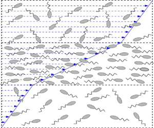
We first discuss the physical mechanism underlying the proposed instability (illustrated through a schematic in figure 1). In the rest of the paper, the instability is demonstrated through a linear stability analysis, followed by the results of nonlinear simulations. Both the analysis and simulations pertain to a bacterial suspension subjected (on average) to a simple shear flow, and are restricted to perturbations that only vary along the gradient direction of the ambient shear. The bacteria are modelled as slender particles that swim along their axis, while being rotated and aligned by the background shear. The latter leads to a spatially homogeneous sheared suspension with an anisotropic orientation distribution (figure 1a). In the dilute regime, the contribution of the anisotropically oriented bacteria to the suspension viscosity is proportional to the local concentration. The flow perturbation created by the tail-actuated swimming mechanism of the oriented bacteria (termed ‘pushers’) reinforces the fluid flow along the extensional axis of the imposed shear. Hence, the suspension viscosity is reduced below that of the solvent (Hatwalne et al. Reference Hatwalne, Ramaswamy, Rao and Simha2004; Sokolov & Aranson Reference Sokolov and Aranson2009; Saintillan Reference Saintillan2010; Gachelin et al. Reference Gachelin, Mino, Berthet, Lindner, Rousselet and Clément2013; López et al. Reference López, Gachelin, Douarche, Auradou and Clément2015; Bechtel & Khair Reference Bechtel and Khair2017; Nambiar, Nott & Subramanian Reference Nambiar, Nott and Subramanian2017; Saintillan Reference Saintillan2018; Nambiar et al. Reference Nambiar, Phanikanth, Nott and Subramanian2019b). This is in sharp contrast to suspensions with passive microstructural elements which always resist the imposed shear, leading to an enhanced viscosity (Batchelor Reference Batchelor1970). Now, imagine a spontaneous gradient-aligned perturbation that leads to a lower (higher) effective suspension viscosity in regions of higher (lower) concentration (figure 1b). The restriction to perturbations varying only along the gradient direction, and the assumed inertialess limit, implies that the shear stress is independent of the gradient coordinate ( $z$). This invariance of the shear stress implies that the higher (lower) concentration layers are subject to a higher (lower) shear rate (figure 1d). In the higher shear rate regions, the bacteria are more aligned with the flow and, therefore, have a lower probability of migrating in the gradient direction. In turn, this implies a net drift of bacteria into the higher shear rate (higher concentration) regions. The diffusive motion of bacteria drives an opposing stabilizing flux. The drift overcoming the opposing diffusive flux thus provides a mechanism for exponential growth of gradient-aligned (layering) concentration-shear fluctuations from the homogeneous state (figure 1c). Front-actuated swimmers (‘pullers’) such as algae, and passive rigid rods, increase the suspension viscosity in the dilute regime, leading to a stabilizing drift, and thence, to decaying fluctuations.

Figure 1. Schematic illustrating the physical mechanism of the concentration-banding instability; where  $\mu _s$ is the suspension viscosity, and
  $F_{V}$ and
  $F_{D}$ represent the destabilizing and stabilizing fluxes due to drift and diffusion, respectively. (a) Homogeneously sheared base-state; (b) spontaneous perturbation in the concentration; (c) net accumulation in the high shear region and (d) induced shear rate perturbation.
Migration of bacteria towards higher-shear rate regions, in inhomogeneous shear flows, leading to so-called shear trapping, has been examined before (Rusconi, Guasto & Stocker Reference Rusconi, Guasto and Stocker2014; Barry et al. Reference Barry, Rusconi, Guasto and Stocker2015; Bearon & Hazel Reference Bearon and Hazel2015; Ezhilan & Saintillan Reference Ezhilan and Saintillan2015; Sokolov & Aranson Reference Sokolov and Aranson2016; Vennamneni, Nambiar & Subramanian Reference Vennamneni, Nambiar and Subramanian2020). However, all of these studies have focused on the kinematic point of view where changes in the bacterial concentration and orientation distribution do not couple back to the flow. The mechanism outlined above illustrates, for the first time, how the back-coupling via the bacterial stress leads to exponentially growing concentration and shear rate fluctuations. Eventually, the growing fluctuations lead to a banded steady state, with homogeneous high-shear bands, containing a marginally higher concentration of bacteria relative to the original base-state, and that are separated by an interface depleted of bacteria.
Gradient banding in sheared active fluids has been so far studied using phenomenological continuum equations which allow for a bulk nematic or polar order. In allowing for such an order, these formulations implicitly assume the orientation degrees of freedom to evolve on a slow time scale (Cates et al. Reference Cates, Fielding, Marenduzzo, Orlandini and Yeomans2008; Giomi, Liverpool & Marchetti Reference Giomi, Liverpool and Marchetti2010; Fielding, Marenduzzo & Cates Reference Fielding, Marenduzzo and Cates2011; Marchetti et al. Reference Marchetti, Joanny, Ramaswamy, Liverpool, Prost, Rao and Simha2013; Loisy et al. Reference Loisy, Eggers and Liverpool2018). Even in cases where concentration (position) degrees of freedom are incorporated, both the orientation and concentration modes are assumed to evolve on comparably slow time scales (see for instance Giomi, Marchetti & Liverpool Reference Giomi, Marchetti and Liverpool2008). In contrast, in the context of explaining shear-induced migration of bacteria and algae in dilute suspensions (Rusconi et al. Reference Rusconi, Guasto and Stocker2014; Barry et al. Reference Barry, Rusconi, Guasto and Stocker2015), it has been shown that the concentration degrees of freedom do evolve on a slower time scale, while the orientation degrees of freedom evolve much faster, and may then be treated in a quasi-steady approximation (Bearon & Hazel Reference Bearon and Hazel2015; Vennamneni et al. Reference Vennamneni, Nambiar and Subramanian2020). Thus, the phenomenological active fluids approach is not expected to describe shear-induced migration in dilute swimmer suspensions. To the extent that the concentration-shear coupling mechanism described above (figure 1) relies crucially on the shear-induced migration from a lower to a higher concentration layer, the banding instability also lies outside the purview of the aforementioned phenomenological approach. Indeed, earlier results in the literature only report the shear-modified orientation instability leading to collective motion (or bacterial turbulence), already seen in unsheared active fluids (Cates et al. Reference Cates, Fielding, Marenduzzo, Orlandini and Yeomans2008; Marchetti et al. Reference Marchetti, Joanny, Ramaswamy, Liverpool, Prost, Rao and Simha2013; Loisy et al. Reference Loisy, Eggers and Liverpool2018). In the specific context of sheared bacterial suspensions, an earlier effort only examined vorticity-aligned perturbations, and therefore did not find the novel concentration-shear instability analysed here (Pahlavan & Saintillan Reference Pahlavan and Saintillan2011). To the best of our knowledge therefore, this is the first demonstration of a shear-induced mechanism for enhanced fluctuations, leading to gradient banding in an active fluid.
The paper is organized as follows. Section 2 describes the system of equations governing the bacterial suspension. The approach used here is based on the Stokes–Smoluchowski framework, and accordingly, § 2.1 briefly discusses the relative merits of the Landau–deGennes (consisting of the phenomenological active-fluid equations mentioned above) and Stokes–Smoluchowski approaches that have most often been used to examine the dynamics of active fluids, including bacterial suspensions. Section 3 outlines the linear stability analyses (§§ 3.1 and 3.2) and the nonlinear simulations (§ 3.3). In § 3.1, a multiple scale analysis is used to obtain a semi-analytical expression for the growth rate of concentration perturbations in the limit where the time scales for orientation and spatial degrees of freedom are well separated. Next, in § 3.2, a full linear stability analysis numerically obtains the growth rate of coupled concentration–orientation perturbations, without any restriction on the underlying time scales. Section 3.3 examines the one-dimensional gradient-banded steady states seen in the nonlinear simulations. In § 3.4, we compare our results with a recent experiment studying the rheology of dilute bacterial suspensions (Martinez et al. Reference Martinez, Clément, Arlt, Douarche, Dawson, Schwarz-Linek, Creppy, Škultéty, Morozov and Auradou2020). Finally, in § 4, we present the conclusions, while discussing the future scope of this work.
2. Theoretical model
At the microscale, a bacterium swims with a speed  $U_b$, and the swimming direction (
 $\,\boldsymbol {p}$) decorrelates via both rotary diffusion (with diffusivity
  $D_r$) and tumbling (at a mean rate
  $\tau ^{-1}$). Using
  $\tau$ and the length (
 $H$) and velocity scale (
 $U_{\infty }$) of the imposed flow as the time, length and velocity scales, respectively, the non-dimensional kinetic equation for the bacterium phase-space probability density,
  $\varOmega (\boldsymbol {x},\boldsymbol {p},t)$ in the dilute limit is given by
 \begin{equation} \frac{\partial \varOmega}{\partial t} + (\epsilon \boldsymbol{p} + Pe \boldsymbol{u})\boldsymbol{\cdot} \boldsymbol{\nabla}_{\boldsymbol{x}}\varOmega-\tau D_r \nabla^{2}_{p}\varOmega+Pe \boldsymbol{\nabla}_{p} \boldsymbol{\cdot} (\dot{\boldsymbol{p}}\varOmega) +\left[\varOmega- \frac{1}{4{\rm \pi}} \int \textrm{d} \boldsymbol{p}^{\prime} \varOmega(\boldsymbol{p}^{\prime})\right]=0, \end{equation}
where  $\epsilon = U_b\tau /H$ is the ratio of the bacterium run length to the imposed length scale,
  $Pe = U_{\infty }\tau /H$ denotes the relative importance of the shear-induced and intrinsic reorientation time scales and
  $\tau D_r$ gives the relative importance of tumbling and rotary diffusion. In (2.1),
  $\boldsymbol {u}$ is the convecting suspension velocity field. Approximating the bacteria as slender force-dipoles, the rotation due to shear flow is given by the Jeffery relation,
  $\dot {\boldsymbol {p}}=\boldsymbol {E} \boldsymbol {\cdot } \boldsymbol {p}+\boldsymbol {\omega } \boldsymbol {\cdot } \boldsymbol {p}-\boldsymbol {p}(\boldsymbol {E}: \boldsymbol {p} \boldsymbol {p})$, where
  $\boldsymbol {E}$ and
  $\boldsymbol {\omega }$ are the strain rate and vorticity tensors, respectively, associated with the local linear flow (Jeffery Reference Jeffery1922). As discussed in the introduction, this rotation due to the flow, coupled with swimming, leads to a migration of the bacteria towards the high shear rate regions.
Equation (2.1) is coupled to the inertialess momentum and continuity equations which govern the suspension flow ( $\boldsymbol {u}$), and are given by:
 \begin{gather} \boldsymbol{\nabla} \boldsymbol{\cdot} \boldsymbol{\varSigma} - \boldsymbol{\nabla} P =0 \implies Pe \nabla^{2} \boldsymbol{u}=-\boldsymbol{\nabla} \boldsymbol{\cdot} \boldsymbol{\varSigma}^{B} +\boldsymbol{\nabla} P, \end{gather}
 \begin{gather}\boldsymbol{\nabla} \boldsymbol{\cdot} \boldsymbol{u}=0, \end{gather}
where  $P$ is the suspension pressure and
  $\boldsymbol {\varSigma }$ the suspension stress;
  $\boldsymbol {\varSigma }$ is a sum of the solvent and active stresses,
  $\boldsymbol {\varSigma } = \boldsymbol {\varSigma }^{B} +Pe (\boldsymbol {\nabla } \boldsymbol {u} +\boldsymbol {\nabla } \boldsymbol {u}^{\textrm {T}})$, where the stress is scaled by
  $\mu \tau ^{-1}$ with
  $\mu$ being the solvent viscosity. The active stress,
  $\boldsymbol {\varSigma }^{B}$, is the coarse-grained stress exerted by the particle-phase (bacteria) (Batchelor Reference Batchelor1970). We approximate
  $\boldsymbol {\varSigma }^{B}$ by its active contribution alone which, in a continuum framework, is given in terms of the bacterium force-dipole density as
  $-\mathcal {A} \int \textrm {d}\boldsymbol {p} \varOmega (\boldsymbol {p})(\boldsymbol {p}\boldsymbol {p}-I/3)$. The non-dimensional parameter
  $\mathcal {A}=\mathcal {C} n_0 L^{2}U_{b}\tau$ is the activity number; here,
  $L$ is the bacterium length,
  $n_0$ the number density and
  $\mathcal {C}$ the non-dimensional strength of the intrinsic bacterium force-dipole, with
  $\mathcal {C}>0$ for ‘pushers’ (Koch & Subramanian Reference Koch and Subramanian2011). The active stress is known to reduce the suspension viscosity (Saintillan Reference Saintillan2018), an effect that is crucial to the banding instability analysed here. As will be seen in § 3, the parameters
  $\mathcal {A}$ and
  $Pe$ delineate the region of instability. In the general case,
  $\boldsymbol {\varSigma }^{B}$ has an additional passive stress contribution arising from the bacterium inextensibility. For moderate
  $Pe$, the regime of interest in this work, the passive stress only acts as an enhanced viscosity. Since this effect has been examined before (Subramanian & Koch Reference Subramanian and Koch2009), here, we neglect it in order to focus on the active stress and concentration coupling.
2.1. The Landau–deGennes and the Stokes–Smoluchowski frameworks
Having summarized the theoretical framework above, it is worth drawing a distinction between the two classes of theoretical models that have been used in the literature to analyse active fluids, bacterial suspensions in particular. The first class of models is based on the phenomenological active-fluid formalism which originated in passive liquid crystal hydrodynamics (De Gennes & Prost Reference De Gennes and Prost1993). In the original passive version, the equations of motion for the order parameter (nematic or polar orientational order, for instance) were derived based on postulating a free energy functional with the constituent terms postulated based on symmetry arguments. The resulting free energy allows for the onset of bulk orientational order above a threshold volume fraction (under quiescent conditions). This approach has been modified for active fluids with the addition of so-called prohibited terms to the stress and order parameter evolution equations. While the latter addition only serves to renormalize the aforementioned threshold for transition to orientational order, the additional term in the stress leads to a fundamentally new dynamics (Simha & Ramaswamy Reference Simha and Ramaswamy2002; Hatwalne et al. Reference Hatwalne, Ramaswamy, Rao and Simha2004; Marchetti et al. Reference Marchetti, Joanny, Ramaswamy, Liverpool, Prost, Rao and Simha2013). These equations have since been solved under different circumstances (Cates et al. Reference Cates, Fielding, Marenduzzo, Orlandini and Yeomans2008; Giomi et al. Reference Giomi, Marchetti and Liverpool2008, Reference Giomi, Liverpool and Marchetti2010; Fielding et al. Reference Fielding, Marenduzzo and Cates2011; Loisy et al. Reference Loisy, Eggers and Liverpool2018). The approach has been very successful in explaining a host of novel phenomena across a range of systems all of which come under the general umbrella of active matter (Sanchez et al. Reference Sanchez, Chen, DeCamp, Heymann and Dogic2012; Marchetti et al. Reference Marchetti, Joanny, Ramaswamy, Liverpool, Prost, Rao and Simha2013; Doostmohammadi et al. Reference Doostmohammadi, Ignés-Mullol, Yeomans and Sagués2018); for bacterial suspensions in particular, the results are quite representative at high volume fractions (Wensink et al. Reference Wensink, Dunkel, Heidenreich, Drescher, Goldstein, Löwen and Yeomans2012; Li et al. Reference Li, Shi, Huang, Chen, Xiao, Liu, Chaté and Zhang2019).
In contrast, the second approach, the one adopted in the present manuscript, is suited to dilute suspensions of run-and-tumble and rotary diffusing swimmers (bacteria being a specific example), and thereby, is complementary to the above approach based on the liquid crystal phenomenology. This approach may be termed the Stokes–Smoluchowski framework since, as seen above, the kinetic equation for the bacterial probability density resembles the Smoluchowski equation for Brownian particles (except that the original diffusional relaxation is now complemented by an additional run-and-tumble-driven relaxation). The Smoluchowski equation is coupled to the Stokes equations via the bacterial stress. While restricted in its applicability (to the dilute regime), the model can be derived from first principles, wherein interactions between the bacteria are only retained at a mean-field level (Saintillan & Shelley Reference Saintillan and Shelley2008a,Reference Saintillan and Shelleyb; Subramanian & Koch Reference Subramanian and Koch2009; Koch & Subramanian Reference Koch and Subramanian2011; Stenhammar et al. Reference Stenhammar, Nardini, Nash, Marenduzzo and Morozov2017). As a result the model contains no phenomenological approximations and all the parameters involved can be directly measured in experiments. As already mentioned above, the model has been shown to accurately predict concentration inhomogeneities, resulting from shear-induced migration, in channel flows (Bearon & Hazel Reference Bearon and Hazel2015; Vennamneni et al. Reference Vennamneni, Nambiar and Subramanian2020).
While the active-fluid formalism has been applied with considerable success to dense active suspensions, its inapplicability in the dilute regime may be seen from the Frank elastic terms, in the free energy functional, that drive a diffusive relaxation of the order parameter. Such diffusive relaxation may arise from short-range repulsive (excluded volume) interactions between closely spaced bacteria at high volume fractions; there is, however, no notion of such an ‘elastic network’ formed by bacteria in the dilute regime. Moreover, the diffusive relaxation becomes arbitrarily weak at sufficiently long wavelengths, and as a result, the threshold for the onset of collective motion in a quiescent bacterial suspension, when analysed using the active-fluid formalism, becomes system-size dependent; the threshold scaling as the inverse square of the system size, implying that a bacterial suspension in a large enough domain is always unstable (Simha & Ramaswamy Reference Simha and Ramaswamy2002; Marchetti et al. Reference Marchetti, Joanny, Ramaswamy, Liverpool, Prost, Rao and Simha2013). In contrast, the Stokes–Smoluchowski approach leads to a threshold volume fraction that is only a function of the bacterium swimming parameters; in fact, the threshold may be stated in terms of the activity number defined above, and is given by  $\mathcal {A}^{*} = 5(1+ 6\tau D_r)$ (Subramanian & Koch Reference Subramanian and Koch2009). This threshold has been validated in a recent experiment (Martinez et al. Reference Martinez, Clément, Arlt, Douarche, Dawson, Schwarz-Linek, Creppy, Škultéty, Morozov and Auradou2020), which also discuss the inappropriateness of the aforementioned system-size-dependent threshold. A detailed comparison between the observations of Martinez et al. (Reference Martinez, Clément, Arlt, Douarche, Dawson, Schwarz-Linek, Creppy, Škultéty, Morozov and Auradou2020) and results obtained in this paper is carried out in § 3.4. Note that a relaxation driven by Frank elasticity would require redefining the activity number with
  $\tau$ being replaced by
  $L_{sys}^{2}/D_t$,
  $L_{sys}$ here being the system size and
  $D_t$ the diffusivity proportional to the Frank elastic constant. The resulting threshold volume fraction may then be written in the form
  $(n_0L^{3}) \sim D_t L/(UL_{sys}^{2})$, leading to the inverse-square system-size scaling mentioned above.
To summarize then, the Stokes–Smoluchowski framework used here is appropriate for the dilute bacterial suspensions under consideration; higher volume fractions would necessarily require the phenomenological approach based on the active-fluid formalism above. Use of this latter formalism in the dilute regime can lead to incorrect results since the phenomenological constants involved do not have a direct microscopic interpretation in the dilute limit. To reiterate, in this paper we use the Stokes–Smoluchowski framework which is more appropriate for the aforementioned experiments where novel behaviour is seen at volume fractions as low as  $0.75\,\%$ (see § 3.4). It should be noted that the kinetic equation (2.1), that lies at the heart of this framework, does not therefore include either direct hydrodynamic or steric interactions between the swimming bacteria. While recent efforts have analysed pairwise hydrodynamic interactions in the Stokes–Smoluchowski framework, this lies beyond the scope of the current effort (Stenhammar et al. Reference Stenhammar, Nardini, Nash, Marenduzzo and Morozov2017; Nambiar, Garg & Subramanian Reference Nambiar, Garg and Subramanian2019a).
3. Results and discussion
The homogeneous base-state is given by  $\boldsymbol {u}_{0}=z \boldsymbol {1_x}$ and an anisotropic orientation distribution
  $\varOmega _{0}(\boldsymbol {p})$, which needs to be solved for numerically; the numerical method is described in appendix A. Knowing
  $\varOmega _0(\boldsymbol {p})$ allows for the calculation of the stress–shear rate curves for the homogeneous state. Figures 2(a) and 2(b) show the variation of the suspension shear stress (
 $\varSigma _0$) and the suspension viscosity (
 $\mu _{s0}$) with
  $Pe$, respectively. For
  $\mathcal {A} <\mathcal {A}^{*}$, the suspension shear stress in the base-state (
 $\varSigma _{0}$) is a monotonically increasing function of the shear rate although the effective viscosity is lower than the solvent viscosity;
  $\mathcal {A}^{*} \approx 35$ marks the threshold for the instability in an unsheared suspension owing to the viscosity vanishing at
  $Pe=0$ (Subramanian & Koch Reference Subramanian and Koch2009). For
  $\mathcal {A} >\mathcal {A}^{*}$,
  $\varSigma _{0}$ is a non-monotonic function of
  $Pe$ and the suspension has a zero viscosity at
  $Pe \equiv Pe_{cr}(\mathcal {A})$;
  $Pe_{cr}$ being an increasing function of
  $\mathcal {A}$, with
  $Pe_{cr}(\mathcal {A}^{*})$ = 0. We examine the stability of this homogeneous state to gradient-aligned perturbations in the velocity field
  $(u_{1})$ and orientation distribution
  $(\varOmega _1)$. Since gradient-aligned perturbations are the long-time limit for almost any initial wavevector in simple shear flow, the assumption of gradient alignment is not restrictive.

Figure 2. A sheared bacterial suspension with  $\tau D_r=1$. (a) The variation of the homogeneous base-state stress with
  $Pe$. (b) The variation of suspension viscosity with
  $Pe$. (c) The growth rate of layering perturbations, predicted by the multiple scale analysis, versus
  $Pe$. (d) The unstable interval of
  $Pe$ values, corresponding to the concentration-shear instability, in the
  $\mathcal {A}$–
 $Pe$ plane. The
  $Pe$ values marking the endpoints of the unstable interval are
  $Pe_{cr}$ (corresponding to an infinite growth rate) and
  $Pe_{max}$ (corresponding to a zero growth rate); the
  $Pe_{cr}$ and
  $Pe_{max}$ values are also marked in (a).
In what follows, we examine the linear stability of gradient-aligned concentration perturbations alone in § 3.1 via a multiple scale analysis, the linear stability of all gradient-aligned perturbations in § 3.2 and finally, the fully nonlinear evolution of such perturbations in § 3.3. The bacterial suspension is assumed to be unbounded in extent in all of the above. Confinement of swimmer suspensions is known to lead to concentration inhomogeneities via wall accumulation of swimming bacteria through both kinematic and hydrodynamic mechanisms (Berke et al. Reference Berke, Turner, Berg and Lauga2008; Drescher et al. Reference Drescher, Dunkel, Cisneros, Ganguly and Goldstein2011; Elgeti & Gompper Reference Elgeti and Gompper2016). However, in order to focus on concentration inhomogeneities arising from banding in the bulk, we neglect wall effects in the analysis, and impose periodic boundary conditions in the gradient direction in both the stability analysis and the simulations.
3.1. Concentration dynamics (CD)
In the limit  $\epsilon = U_b\tau /H \rightarrow 0$, concentration fluctuations (
 $n_1=\int \varOmega _1 \, \textrm {d}\boldsymbol {p}$) evolve on a slower, diffusive, time scale (
 $t_{2}\sim \textit{O}$(
 $H^{2}/(\tau U^{2}_{b}$))) compared to orientation fluctuations (
 $t_{1}\sim \textit{O}$(
 $\tau$)). Using a multiple time scale formalism,
  $\varOmega _1$ may, in this limit, be expanded as
 \begin{equation} \varOmega_1 = \varOmega_{10}(\boldsymbol{p}, t_1) n_1(z, t_2) + \epsilon \varOmega_{11}(\boldsymbol{p}, t_1)+ \epsilon^2 \varOmega_{12}(\boldsymbol{p}, t_1). \end{equation}
The orientation degrees of freedom evolve quasi-statically on the time scales of interest ( $t_2/t_1 \sim O(1/\epsilon ^{2}) \gg 1$), and a reduced equation governing
  $n_1$ can be derived as (see appendix B.1; Subramanian & Brady Reference Subramanian and Brady2004; Kasyap & Koch Reference Kasyap and Koch2014; Vennamneni et al. Reference Vennamneni, Nambiar and Subramanian2020)
 \begin{equation} \frac{\partial n_1}{\partial t_{2}}= \frac{\partial}{\partial z} \left(-V_1+D_0 \frac{\partial n_1}{\partial z} \right). \end{equation}
The concentration perturbations ( $n_1$) are thus governed by a drift-diffusion equation. The combination of swimming and orientation decorrelation results in the swimmers undergoing a diffusive motion for long times, with an effective diffusivity
  $D_0$, in (3.2). In the absence of flow, the effective diffusivity can be analytically obtained as
  $D_0 =1/(3(1+2\tau D_r))$ (see, for instance, Krishnamurthy & Subramanian Reference Krishnamurthy and Subramanian2015). In the presence of flow, the effective diffusivity also depends on the Péclet number and needs to be calculated numerically; the procedure is outlined in appendix B.1. The differential rotation due to the inhomogeneous perturbed shear flow leads to the additional drift term,
  $V_1$, in (3.2). As shown in appendix B.1, the drift term is proportional to the perturbation shear rate gradient and given by,
 \begin{equation} V_1 = 2 \sqrt{\frac{\rm \pi}{3}} e_{1,0} \frac{\partial \dot{\gamma}_1}{\partial z}, \end{equation}
where  $e_{1,0}$ is representative of the magnitude of the drift.
  $e_{1,0}$ is a function of
  $\tau D_r$ and
  $Pe$ and is obtained numerically (see appendix B.1). We find that
  $e_{1,0}>0$ and thus the drift is directed from low to high shear rate regions. As explained in the introduction, the sign of the drift is rationalized by noting that swimmers in the high shear rate regions are more aligned with the flow and hence have a lesser probability of migrating in the gradient direction when compared to swimmers in the low shear rate regions. Hence, the drift drives a destabilizing flux from regions of low to high shear rate (figure 1). The diffusive contribution (
 $D_0>0$) (the second term in (3.2)), on the other hand, drives an opposing flux that is stabilizing.
The perturbation shear rate ( $\dot {\gamma }_1$) in (3.3) is obtained from the momentum equation as
 \begin{equation} (Pe \mu_{s0}) \frac{\partial \dot{\gamma}_1}{\partial z} = \frac{\partial n_1}{\partial z} \vert \varSigma^{B}_0 \vert, \end{equation}
where  $\mu _{s0}$ is the suspension viscosity and
  $\varSigma ^{B}_0$ the active shear stress in the homogeneous state; the respective expressions are given in appendix B.1. Assuming normal modes of the form
  $[n_1,\dot {\gamma }_{1}]=[\tilde {n}_1, \tilde {\dot {\gamma }}_{1}] \cos (zk_{z})\exp (\sigma t_{2})$, we obtain the following semi-analytical expression for the eigenvalue governing the evolution of concentration perturbations
 \begin{equation} \sigma=k_{z}^{2} \left( 2\sqrt{\frac{\rm \pi}{3}} e_{1,0} \frac{\vert \varSigma^{B}_0 \vert}{Pe \mu_{s0}}-D_{0} \right). \end{equation}
 When the first term in (3.5), denoting the destabilizing drift, exceeds the diffusivity,  $\sigma >0$, and the homogeneous state becomes unstable (figure 2c). For
  $Pe \rightarrow Pe_{cr}$, the suspension viscosity (
 $\mu _{s0}$) vanishes and the destabilizing drift diverges in (3.5), making the suspension infinitely susceptible to growing concentration fluctuations (figure 2c). The lower (
 $Pe_{cr}$) and upper (
 $Pe_{max}$) Péclet thresholds for the concentration-shear instability as a function of
  $\mathcal {A}$ are shown in figure 2(d), with the range of (dimensionless) unstable shear rates
  $(Pe_{cr}, Pe_{max})$ increasing with increasing
  $\mathcal {A}$.
3.2. Coupled concentration and orientation dynamics (CCOD)
The divergence of the growth rate for  $Pe \rightarrow Pe_{cr}^{+}$, seen in figure 2(c), is an artefact of the multiple scale analysis. As
  $Pe$ approaches
  $Pe_{cr}$, the time scale (defined as the inverse of the growth rate) characterizing the concentration perturbations decreases, until for
  $Pe$ sufficiently close to
  $Pe_{cr}$, the growth rate
  $\sigma \sim \tau ^{-1}$, or alternatively, the wavenumber in the gradient direction,
  $k_z \sim (U_b \tau )^{-1}$, and the assumed separation of scales between the concentration and orientation fluctuations is no longer present. The predictions of the multiple scale analysis are thus invalidated for
  $Pe$ sufficiently close to
  $Pe_{cr}$. In order to analyse the behaviour of perturbations across
  $Pe = Pe_{cr}$, we therefore carry out a linear stability analysis without the assumption of a time scale separation. The complete eigenspectrum, corresponding to any small-amplitude perturbation aligned along the gradient direction, is obtained numerically by expanding the relevant fields in spherical harmonics. The details of the numerical method are given in appendix B.2.
Figure 3 (inset) shows good agreement between the two approaches (the multiple scale and the full linear stability analyses) for  $Pe > Pe_{cr}$. Importantly, the full analysis continues to predict a finite growth rate of
  $\textit{O}(1/\tau )$ for
  $Pe \rightarrow Pe_{cr}$. The multiple scale analysis also does not predict a finite length scale for the fastest growing mode since
  $\sigma \propto k_z^{2}$ (see (3.5)), so that the shortest-wavelength modes are predicted to grow at the fastest rates. In contrast, the full stability analysis, with the orientation dynamics included, predicts the fastest growing wavenumber to be
  $\textit{O}(1/(U_b\tau ))$ such that the relaxation times of the concentration and orientation (and thence, stress) fluctuations become comparable, both being
  $\textit{O}(\tau )$ (see figure 4a). For
  $k_z>\textit{O}(1/(U_b\tau ))$, the diffusive rate of accumulation of bacteria (
 $k_z^{-2}/(\tau U^{2}_b$)) would exceed the stress relaxation time (
 $\tau$), and hence, such perturbations decay.


Figure 4. Variation in the (a) growth rate and (b) the amplitude of concentration fluctuations ( $\tilde {n}_{1}$) as a function of the wavenumber for different
  $Pe$ with
  $\tau D_r=1$,
  $\mathcal {A}=48.5$ (
 $Pe_{cr} \approx 2.29$ and
  $Pe_{max} \approx 3.1$). Here, the growth rate (
 $\sigma$) and the wavenumber (
 $k_z$) are non-dimensionalized using the bacterium tumble time
  $\tau$ and run length
  $U_b \tau$, respectively.
The full analysis also predicts the orientation-shear instability, which has earlier been interpreted as a negative-viscosity instability responsible for the onset of collective motion (bacterial turbulence) in a quiescent bacterial suspension. The orientation-shear instability has been studied earlier in the absence of an imposed shear ( $Pe = 0$). It is a long-wavelength instability, with
  $k_z =0$ being the most unstable mode, and having a finite growth rate. The longest-wavelength perturbations may be regarded as homogeneous shearing flows, on the scale of the bacterium swimming motion, and the response to this homogeneous shear may then be interpreted in terms of the aforementioned negative viscosity (see discussion in § 3.1 of Subramanian & Koch Reference Subramanian and Koch2009). Importantly, the unstable eigenfunction is spatially homogeneous, implying that concentration fluctuations are absent at the onset of the orientation-shear instability (Underhill et al. Reference Underhill, Hernandez-Ortiz and Graham2008;Subramanian & Koch Reference Subramanian and Koch2009). These features are in contrast with the concentration-shear instability described here.
In light of the aforementioned discussion, one thus needs to distinguish between the orientation-shear and concentration-shear instability mechanisms which operate in distinct parameter regimes. The instability onset, regardless of the mechanism, coincides with the stress becoming a non-monotonic function of the shear rate – this corresponds to the curves for  $\mathcal {A} > \mathcal {A}^{*}$ in figure 2(a). For
  $\mathcal {A} > \mathcal {A}^{*}$, figure 3 shows that orientation fluctuations drive an instability on the negative-viscosity portion of the stress–shear rate curve corresponding to
  $Pe < Pe_{cr}$, with this orientation-shear instability arising due to a negative apparent viscosity, as mentioned above, and being the equivalent of the mechanical shear-banding instability known from earlier investigations of passive complex fluids (Cates & Fielding Reference Cates and Fielding2006); the novel concentration-shear instability exists only on the positive-viscosity branch of the stress–shear curve corresponding to
  $Pe_{cr} < Pe < Pe_{max}$.
The two instabilities are most easily be differentiated by focusing on the behaviour of the spatially homogeneous ( $k_z=0$) mode since it corresponds to pure orientation fluctuations without associated concentration fluctuations. For the orientation-shear instability at
  $Pe=0$ the most unstable eigenfunction is known to be spatially homogeneous (with
  $k_z=0$) from earlier work (Underhill et al. Reference Underhill, Hernandez-Ortiz and Graham2008; Subramanian & Koch Reference Subramanian and Koch2009). Figure 4(a) shows that the
  $k_z=0$ mode remains the fastest growing perturbation in the presence of a weak shear (‘weak’ here corresponding to the interval
  $Pe <Pe_{cr}$), and hence the growth may be regarded as being due to a mechanism analogous to the original orientation-shear instability. As argued in Subramanian & Koch (Reference Subramanian and Koch2009), the growth arises because bacteria orient, in response to a long-wavelength perturbation, so that the resulting bacterium flow fields reinforce the original perturbation; as stated above, this reinforcing mechanism may be interpreted in terms of a negative viscosity. In stark contrast, figure 4(a) shows that for
  $Pe > Pe_{cr}$, the
  $k_z=0$ mode is stable and the most unstable eigenfunction now has a spatially modulated structure (a finite
  $k_z$) corresponding to a layering perturbation. Thus, in the interval
  $Pe_{cr} < Pe < Pe_ {max}$, the mechanism underlying the growth involves the concentration-shear coupling discussed earlier. For
  $Pe$ in the neighbourhood of
  $Pe_{cr}$, there is no sharp distinction between the two instability mechanisms.
Further insight into the distinction between the two instability mechanisms may be obtained from the behaviour of the long-wavelength number density perturbations ( $\tilde {n}_{1}$) shown in figure 4(b). In an unsheared suspension, the unstable eigenfunction does not have number density perturbations for any
  $k_z$ (the curve in figure 4(b) for
  $Pe=0$) in agreement with earlier predictions (Underhill et al. Reference Underhill, Hernandez-Ortiz and Graham2008; Subramanian & Koch Reference Subramanian and Koch2009). Figure 4(b) shows that weak shear only leads to weak long-wavelength number density perturbations (
 $\tilde {n}_{1} \rightarrow 0$ as
  $k_z \rightarrow 0$) for
  $Pe < Pe_{cr}$. However, the behaviour of these number density perturbations is significantly altered for
  $Pe > Pe_{cr}$. For
  $Pe > Pe_{cr}$, there are strong, long-wavelength concentration fluctuations as predicted by the mechanism outlined earlier. This is seen in figure 4(b) where the amplitude of these fluctuations
  $\tilde {n}_{1}$ now approaches a finite value even as
  $k_z \rightarrow 0$ (with
  $\tilde {n}_{1} =0$ for
  $k_z =0$ being a singular limit). Along with the results of the multiple scale analysis in § 3.1, this clearly shows that it is the concentration-shear coupling mechanism that leads to an instability for
  $Pe> Pe_{cr}$.
3.3. Nonlinear simulations
To examine the steady state resulting from the linear instability discussed above, we numerically integrate (2.1) and (2.3) in time. The nonlinear simulations are carried out in two dimensions, so the orientation vector is restricted to the unit circle, and may be characterized by a single azimuthal angle. A standard spectral formulation is used for the simulations and the details are given in appendix C. The simulation results are validated by comparing against the linear stability analysis during the initial phase of exponential growth (see appendix C). The imposed non-dimensional shear rate ( $Pe$) is taken to be the control parameter.
Figure 5(a–c) shows the evolution of the velocity, shear rate and concentration fields over time for  $Pe = 0.75$ and
  $\mathcal {A}=62.83$ with
  $\tau D_r=0.0025$. For this choice of parameters,
  $Pe_{cr} \approx 0.67$ and
  $Pe_{max} \approx 0.975$, so that the chosen
  $Pe$ lies in the concentration-shear instability regime. The chosen initial condition is given in appendix C. The velocity field evolves from the initial near-homogeneous shear to a banded steady state, with equal and opposite shear rates in two (unequal) bands, for long times. From figure 5(b), the shear rates selected in the bands are seen to be
  $\dot {\gamma }^{\star } \approx 1.69$ and
  $-\dot {\gamma }^{\star }$. The associated concentration field shows that the two shear bands are homogeneous at steady state, with a localized depletion of bacteria only at the interface between the bands (see figure 5c), this depletion being consistent with earlier findings of high-shear trapping in inhomogeneous shearing flows (Rusconi et al. Reference Rusconi, Guasto and Stocker2014; Bearon & Hazel Reference Bearon and Hazel2015; Vennamneni et al. Reference Vennamneni, Nambiar and Subramanian2020). Note that, despite the appearance, there are only two bands (and one shear interface) at steady state, and not three, since the profiles may be shifted by an arbitrary amount in the gradient direction on account of the periodic boundary conditions. Figure 6 shows the time evolution of the associated suspension stress for different
  $Pe$, including the case
  $Pe = 0.75$ examined in figure 5. For all cases, the suspension stress asymptotes to zero for long times. Figure 7(a–c) shows the steady-state velocity, shear rate and concentration fields for varying
  $Pe$. Thus, for all
  $Pe$ examined, a gradient-banded state results for long times; two bands with differing shear rates coexist at the same (zero) shear stress. The selected shear rate in the bands is seen to be independent of
  $Pe$. In light of figure 6, the only criterion controlling the shear rate selected at steady state is that of the shear stress being zero. As a result, the only consequence of varying the imposed shear rate is to alter the relative widths of the two shear bands in a manner so as to accommodate the imposed shear. For
  $Pe = 0$ alone, the two bands have equal thicknesses, each occupying half the simulation domain.

Figure 5. The time evolution of (a) the velocity ( $u$), (b) shear rate (
 $\dot {\gamma }$) and (c) concentration (
 $n$) fields towards the gradient banded steady state for
  $Pe =0.75$. The simulations have a box size 10 times the run length
  $U_b \tau$ with
  $\tau D_r=0.0025$ and
  $\mathcal {A}=62.83$; for these parameters,
  $Pe_{cr} \approx 0.67$ and
  $Pe_{max} \approx 0.975$. The shear rates
  $\dot {\gamma }^{\star }$ and
  $-\dot {\gamma }^{\star }$ are also marked as dashed lines in (b).

Figure 6. The time evolution of the suspension shear stress ( $\varSigma$) for various
  $Pe$. The simulations have a box size 10 times the run length
  $U_b \tau$ with
  $\tau D_r=0.0025$ and
  $\mathcal {A}=62.83$; for these parameters,
  $Pe_{cr} \approx 0.67$ and
  $Pe_{max} \approx 0.975$.

Figure 7. (a) The velocity ( $u$), (b) the shear rate (
 $\dot {\gamma }$) and (c) the concentration (
 $n$) profiles in the nonlinear banded state. The simulations have a box size 10 times the run length
  $U_b \tau$ with
  $\tau D_r=0.0025$ and
  $\mathcal {A}=62.83$; for these parameters,
  $Pe_{cr} \approx 0.67$ and
  $Pe_{max} \approx 0.975$. (d) Maxwell construction showing selected the shear rate (
 $\dot {\gamma }^{\star } \approx 1.69$), with zero stress, selected in the banded state. The shear rates
  $\dot {\gamma }^{\star }$ and
  $-\dot {\gamma }^{\star }$ are also marked as dashed lines in (b).
Further, the steady-state banded profiles do no show any major difference across  $Pe_{cr} (\approx 0.67$ in figure 7) even though concentration fluctuations are crucial for the instability, and therefore, the start-up kinetics for
  $Pe>Pe_{cr}$. We thus see that both the orientation-shear and concentration-shear instabilities, unexpectedly, lead to a similar nonlinear gradient banded state. This insensitivity of the selected stress to concentration coupling is in contrast to shear banding in passive complex fluids, where this coupling leads to an increase in the selected stress with the shear rate (Fielding & Olmsted Reference Fielding and Olmsted2003; Cates & Fielding Reference Cates and Fielding2006).
Having characterized the nature of the inhomogeneous (gradient-banded) steady state, we now show that a geometric construction based on the homogeneous stress–shear rate curve can be used to predict the selected stress and shear rates in this banded state. Figure 7(d) shows the homogeneous stress–shear curve from figure 2(a) together with its (symmetric) extension to negative shear rates. If we assume a homogeneous concentration profile in the banded state, then knowing the magnitude (zero) of the shear stress from figure 6, we can find the corresponding selected shear rates from figure 7(d). The selected shear rates are seen to be  $\dot {\gamma }^{\star }$ and
  $-\dot {\gamma }^{\star }$. Figure 7(d) thus suggests a banded state with equal and opposite shear rates
  $\dot {\gamma }^{\star }$ which supports a zero bulk stress with a homogeneous concentration. Rather remarkably, the shear rate and stress in the banded state closely follow the geometric construction, even though the concentration profile is not completely homogeneous. This construction is seen to be the equivalent of the Maxwell construction used in equilibrium thermodynamics, with the shear rate playing the role of the specific volume in the familiar one-component system. However, unlike equilibrium thermodynamics, the geometric construction cannot be used to predict the shear stress in the banded state (Cates & Fielding Reference Cates and Fielding2006; Dhont & Briels Reference Dhont and Briels2008; Olmsted Reference Olmsted2008).
The equal and oppositely sheared zones in the banded state imply that the shear rate goes through zero at the interface, driving a local depletion of bacteria (Vennamneni et al. Reference Vennamneni, Nambiar and Subramanian2020) as seen in figure 7(c). The Maxwell construction in figure 7(d) is relevant for an infinitely large system in the gradient direction; however, figure 7(c) shows that the bands in a finite system have a marginally higher concentration of bacteria than the original homogeneous state state due to interfacial depletion. Thus, the selected shear rate slightly differs from  $\dot {\gamma }^{\star }$, the value suggested by the Maxwell construction in figure 7(d). This in turn implies that the stress selected is finite, but (very) small in magnitude. The width of the interface between the shear bands is of the order of the bacterium run length
  $(U_b\tau )$, which can be seen from (2.1) to be the length scale governing the spatial decay of stress. With increasing box size, the extent of the interfacial depletion reduces, and the shear rate selected approaches
  $\dot {\gamma }^{\star }$ predicted by the Maxwell construction (not shown).
An analogous result for the selected stress was obtained earlier for extensile active nematics for nematic–nematic banding and no concentration variation (Cates et al. Reference Cates, Fielding, Marenduzzo, Orlandini and Yeomans2008; Fielding et al. Reference Fielding, Marenduzzo and Cates2011). In this approach, the shear rate is exactly the prediction of the Maxwell construction, since there is no concentration variable (Cates et al. Reference Cates, Fielding, Marenduzzo, Orlandini and Yeomans2008). As discussed in § 2.1, the active–nematic formalism, however, has phenomenological constants that do not have a direct microscopic interpretation, and as pointed our earlier, is not expected to work for dilute bacterial suspensions that are far from an isotropic–nematic transition. This is evident from Giomi et al. (Reference Giomi, Liverpool and Marchetti2010) and Loisy et al. (Reference Loisy, Eggers and Liverpool2018) reporting similar stress–shear rate curves and yet very different velocity profiles from those in Cates et al. (Reference Cates, Fielding, Marenduzzo, Orlandini and Yeomans2008) and Fielding et al. (Reference Fielding, Marenduzzo and Cates2011). In contrast, our approach solves the underlying kinetic equation directly and rigorously demonstrates the selection of a banded state even in the dilute regime. Crucially, our results demonstrate that long-range hydrodynamic interactions offer an alternate explanation for experimental observations of a banded state in dilute bacterial suspensions (Martinez et al. Reference Martinez, Clément, Arlt, Douarche, Dawson, Schwarz-Linek, Creppy, Škultéty, Morozov and Auradou2020). A more detailed comparison with recent experimental results follows.
3.4. Comparison with Martinez et al. (Reference Martinez, Clément, Arlt, Douarche, Dawson, Schwarz-Linek, Creppy, Škultéty, Morozov and Auradou2020)
Martinez et al. (Reference Martinez, Clément, Arlt, Douarche, Dawson, Schwarz-Linek, Creppy, Škultéty, Morozov and Auradou2020) have recently studied the rheology of bacterial suspensions by measuring both the viscosity and the velocity profile of a sheared suspension of Escherichia coli using a Couette and cone-plate rheometer, respectively. This dual measurement allows the authors, for the first time, to ascertain the role of collective motion on the measured rheology. The authors examine a range of (small) volume fractions both in the absence and presence of collective motion. At volume fractions less than  $0.75\,\%$, with an imposed shear rate of
  $0.04\ \textrm {s}^{-1}$ (corresponding to the linear response regime with
  $Pe = \dot {\gamma }\tau \ll 1$), they observe that the zero-shear viscosity decreases with increasing volume fraction. The authors verified the absence of collective motion at these volume fractions based on the velocity profile in the cone-plate rheometer being a simple shear. This decrease in the viscosity, in the absence of collective motion, has been explained based on both the Stokes–Smoluchowski (Bechtel & Khair Reference Bechtel and Khair2017; Nambiar et al. Reference Nambiar, Nott and Subramanian2017) and Landau–deGennes (Hatwalne et al. Reference Hatwalne, Ramaswamy, Rao and Simha2004; Cates et al. Reference Cates, Fielding, Marenduzzo, Orlandini and Yeomans2008) frameworks, with the viscosity reduction being dependent on the system size in the latter case. To compare the two predictions, the authors carried out viscosity measurements for different gap sizes in the Couette rheometer. They did not observe any system size dependence, and therefore conclude that the Stokes–Smoluchowski framework is appropriate for explaining the experimental results at the low volume fractions under consideration.
Furthermore, Martinez et al. (Reference Martinez, Clément, Arlt, Douarche, Dawson, Schwarz-Linek, Creppy, Škultéty, Morozov and Auradou2020) are also the first to report the existence of an intrinsic threshold volume fraction for the onset of collective motion. There have been earlier reports of a threshold volume fraction for the onset of collective motion in bacterial suspensions conforming to a thin-film geometry (Sokolov et al. Reference Sokolov, Aranson, Kessler and Goldstein2007; Sokolov & Aranson Reference Sokolov and Aranson2012). However, the thickness of the film was not varied systematically in these experiments, and thus there was no way of inferring system-size dependence. In contrast, Martinez et al. (Reference Martinez, Clément, Arlt, Douarche, Dawson, Schwarz-Linek, Creppy, Škultéty, Morozov and Auradou2020) systematically vary the gap size of the Couette rheometer to establish that the threshold volume fraction is indeed independent of the confining system size. As seen in § 2.1, the existence of a system-size independent threshold is one of the central predictions of the Stokes–Smoluchowski framework, and it is therefore of interest to compare the experimental and theoretical thresholds (Subramanian & Koch Reference Subramanian and Koch2009). Martinez et al. (Reference Martinez, Clément, Arlt, Douarche, Dawson, Schwarz-Linek, Creppy, Škultéty, Morozov and Auradou2020) report the onset of collective motion for volume fractions greater than  $0.75\,\%$, the threshold being valid both in the absence of an external flow as well as at a low shear rate of
  $0.04\ \textrm {s}^{-1}$ (used for the aforementioned viscosity measurements). The volume fraction (
 $0.75\,\%$) in the experiments was calculated using the cell body volume and corresponds to a hydrodynamic volume fraction (
 $n_0 L^{3}$) of around
  $5.25$ by assuming an estimate for the bacterium length (
 $L$) of
  $10\ \mathrm {\mu } \textrm {m}$ (Linek et al. Reference Schwarz-Linek, Arlt, Jepson, Dawson, Vissers, Miroli, Pilizota, Martinez and Poon2016). Recall from § 2 that the theoretical model predicts the onset in terms of the non-dimensional activity number,
  $\mathcal {A}=\mathcal {C} n_0 L^{2}U_{b}\tau$. The hydrodynamic volume fraction (
 $n_0 L^{3}$) is the relevant parameter for slender particles, and the threshold hydrodynamic volume fraction is then given as
  $(n_0L^{3})_{c} = (\mathcal {A}^{*}/C) (L/U_b \tau )$. For the E. coli strain used by the authors, the parameters have been estimated as
  $L = 10\ \mathrm {\mu } \textrm {m}$,
  $U_b = 10\ \mathrm {\mu } \textrm {m}\ \textrm {s}^{-1}$,
  $\tau =1\ \textrm {s}$ and
  $\tau D_r =0$ (Linek et al. Reference Schwarz-Linek, Arlt, Jepson, Dawson, Vissers, Miroli, Pilizota, Martinez and Poon2016);
  $\tau D_r =0$ is consistent with Martinez et al. (Reference Martinez, Clément, Arlt, Douarche, Dawson, Schwarz-Linek, Creppy, Škultéty, Morozov and Auradou2020) restricting themselves to the pure run-and-tumble case. Using
  $\mathcal {A}^{*} \sim 5$ for the low
  $Pe$ numbers accessed in the experiment, we thus get
  $n_0 L^{3} = 5/\mathcal {C}$, where
  $\mathcal {C}$ is the strength of the dipole constant. The dipole constant has not been experimentally determined, but is expected to be
  $O(1)$ for typical swimmers, since it is defined by requiring the dimensional force dipole to be
  $\mu UL^{2}$. Thus, for
  $O(1)$ values of
  $\mathcal {C}$, the experimental and theoretical thresholds are indeed in agreement. It should be noted that work on passive fibre suspensions has shown that the dilute Stokes–Smoluchowski framework is applicable up to hydrodynamic volume fractions of around 10 (see for instance chapter 10 in Larson (Reference Larson2013) and Mackaplow & Shaqfeh (Reference Mackaplow and Shaqfeh1998)), and hence the observed threshold lies within the validity of the dilute theory.
Martinez et al. (Reference Martinez, Clément, Arlt, Douarche, Dawson, Schwarz-Linek, Creppy, Škultéty, Morozov and Auradou2020) also show that the suspension viscosity becomes nearly zero and approximately invariant with the volume fraction for volume fractions greater than  $0.75 \%$ (see figure 4a in Martinez et al. Reference Martinez, Clément, Arlt, Douarche, Dawson, Schwarz-Linek, Creppy, Škultéty, Morozov and Auradou2020). Further the velocity profile is no longer simple shear flow. Instead, shear banding is observed such that bands with multiple shear rates are observed at the same shear stress (see figure 4b–g in Martinez et al. Reference Martinez, Clément, Arlt, Douarche, Dawson, Schwarz-Linek, Creppy, Škultéty, Morozov and Auradou2020). Recall from § 3.3 that upon the onset of the orientation-shear instability the theoretical model also predicts shear bands (see figure 7a) and a zero viscosity independent of the volume fraction. Thus, we see that the experimental and simulation results are in qualitative agreement even with the simplifying assumption of only gradient direction variations made in the simulations. Guo et al. (Reference Guo, Samanta, Peng, Xu and Cheng2018) have also reported shear banding in bacterial suspensions at moderate volume fractions recently. However, these experiments were conducted in a highly confined setting with a gap width of 60
  $\mathrm {\mu } \textrm {m}$, and swimmer interactions with boundaries are expected to play a dominant role. Note that, in the experiments of Martinez et al. (Reference Martinez, Clément, Arlt, Douarche, Dawson, Schwarz-Linek, Creppy, Škultéty, Morozov and Auradou2020) above, the threshold was found to approach the prediction of the unbounded-domain theory only for gap sizes larger than 200
  $\mathrm {\mu } \textrm {m}$. Since we ignore the effects of confinement, our results cannot be directly applied to Guo et al. (Reference Guo, Samanta, Peng, Xu and Cheng2018), and can at best serve as a qualitative explanation.
To summarize, we see that the Stokes–Smoluchowski framework used in this paper accurately predicts the threshold for the onset of collective motion observed in recent experiments. The same framework also qualitatively predicts the viscosity and the velocity profiles observed beyond the threshold. Recent work has already shown that this framework accurately describes the rheological properties of bacterial suspensions in the absence of collective motion (Bechtel & Khair Reference Bechtel and Khair2017; Saintillan Reference Saintillan2018; Nambiar et al. Reference Nambiar, Phanikanth, Nott and Subramanian2019b; Martinez et al. Reference Martinez, Clément, Arlt, Douarche, Dawson, Schwarz-Linek, Creppy, Škultéty, Morozov and Auradou2020). Complementing these efforts, our work thus establishes that the Stokes–Smoluchowski framework is appropriate for the examination of the rheological properties of dilute bacterial suspensions across the collective motion threshold.
4. Concluding remarks
We have demonstrated a novel concentration-shear instability mechanism in dilute bacterial suspensions. The proposed instability is reminiscent of the Helfand–Federickson mechanism that explains shear-enhanced concentration fluctuations in concentrated polymer solutions near an equilibrium critical point (Helfand & Fredrickson Reference Helfand and Fredrickson1989; Wu, Pine & Dixon Reference Wu, Pine and Dixon1991; Dixon, Pine & Wu Reference Dixon, Pine and Wu1992; Larson Reference Larson1992; Milner Reference Milner1993; Onuki Reference Onuki2002; Fielding & Olmsted Reference Fielding and Olmsted2003; Cromer et al. Reference Cromer, Villet, Fredrickson and Leal2013; Cromer, Fredrickson & Leal Reference Cromer, Fredrickson and Leal2014). However, dilute bacterial suspensions are far from any critical point and the dynamics of the enhanced concentration fluctuations is crucially reliant on the novel rheological response arising from bacterial activity. We hope that the theoretical results reported here would motivate light scattering experiments examining the dynamics of concentration fluctuations in bacterial suspensions. Similar experiments in polymer solutions have shed considerable light on the nature of the shear-enhanced concentration fluctuations (Wu et al. Reference Wu, Pine and Dixon1991; Dixon et al. Reference Dixon, Pine and Wu1992).
The concentration-shear instability mechanism need not be restricted to a rheological scenario. Observations of collective motion driven by concentration fluctuations near the contact line of an evaporating drop were reported in Kasyap, Koch & Wu (Reference Kasyap, Koch and Wu2014), and in pressure-driven pipe flow in Secchi et al. (Reference Secchi, Rusconi, Buzzaccaro, Salek, Smriga, Piazza and Stocker2016). The generalization of our results to an inhomogeneous shear flow would lead to additional insight into these observations. Although for the imposed linear flow considered here, the concentration fluctuations have been found to vanish in the bulk at steady state, one nevertheless expects them to play a key role in a general non-stationary scenario. Even at steady state, the localized depletion in bacterial concentration at the interface between the homogeneous shear bands, and the resulting localization in the stress, is expected to render the banded-state susceptible to secondary interfacial instabilities (Fielding Reference Fielding2005; Miles et al. Reference Miles, Evans, Shelley and Spagnolie2019).
Finally, the unique ability of shear to enhance concentration fluctuations in active suspensions need not be limited to pushers. The recent identification (Barry et al. Reference Barry, Rusconi, Guasto and Stocker2015), and subsequent explanation (Vennamneni et al. Reference Vennamneni, Nambiar and Subramanian2020) of a low-shear trapping regime, implies that an imposed shear may also be capable of enhancing concentration fluctuations in suspensions of pullers (algae with contractile force dipoles, for instance). The role of concentration fluctuations is expected to be substantial in this case owing to the phenomenon of centreline collapse that has been predicted to occur above a critical swimmer aspect ratio (Vennamneni et al. Reference Vennamneni, Nambiar and Subramanian2020).
Acknowledgements
L.N.R. would like to thank Science and Engineering Research Board, India (Grant No. PDF/2017/002050) and Jawaharlal Nehru Centre for Advanced Scientific Research, Bangalore for the financial support.
Declaration of interests
The authors report no conflict of interest.
Appendix A. The base-state
The bacterium orientation, in the chosen spherical coordinate system, is depicted in figure 8. In the base-state, whose stability we examine in the paper, the bacteria are homogeneously distributed in the gradient direction and have an anisotropic orientation distribution due to rotation by the imposed shear flow. The resulting homogeneous active stress does not induce any fluid flow, and thus the flow field remains identical to the imposed shear,  $\boldsymbol {u}_0=z\boldsymbol {1_{x}}$. The momentum and continuity equations (2.3) are, thus, trivially satisfied. From (2.1), the equation governing the orientation distribution (
 $\varOmega _0$) is
 \begin{equation} Pe \boldsymbol{\nabla}_{p} \boldsymbol{\cdot} (\dot{\boldsymbol{p}}^{'}\varOmega_{0}) + \left[\varOmega_{0}-\int \textrm{d}\boldsymbol{p}^{'} \frac{1}{4{\rm \pi}} \varOmega_{0}(\boldsymbol{p}^{'})\right]-D_r\tau \nabla^{2}_{p}\varOmega_0=0. \end{equation}
Figure 8. Schematic showing the (a) coordinate system for a bacterium with orientation  $\boldsymbol {p}$ (b) a bacterial suspension subjected to simple shear flow.
A.1. Numerical solution of the base-state probability density
Here we describe the numerical scheme for solving (A 1) for the base-state probability density ( $\varOmega _{0}$), and hence, the base-state stress
  $\varSigma _{0}$ (Nambiar et al. Reference Nambiar, Nott and Subramanian2017, Reference Nambiar, Phanikanth, Nott and Subramanian2019b; Vennamneni et al. Reference Vennamneni, Nambiar and Subramanian2020). Considering
  $\boldsymbol {\nabla }_{p} \boldsymbol {\cdot } (\dot {\boldsymbol {p}}^{'}\varOmega _{0})$, the first term in (A 1), substituting
  $\dot {\boldsymbol {p}^{'}}$, and after simplification, one may write
 \begin{align} \boldsymbol{\nabla}_{p}\boldsymbol{\cdot}(\dot{\boldsymbol{p}^{'}}\varOmega_{0}(\boldsymbol{p})) &= \cos^{2} \theta\cos \phi \frac{\partial \varOmega_{0}}{\partial \theta}-\cot \theta \sin \phi \frac{\partial \varOmega_{0}}{\partial \phi}-3\varOmega_{0} \sin \theta \cos \theta \cos \phi \nonumber\\ &= \textrm{i}\cos^{2}\theta \mathcal{L}_{y}(\varOmega_{0})-\textrm{i}\sin \theta \cos \theta \sin \phi\mathcal{L}_{z}(\varOmega_{0})-3\sin \theta \cos \theta \cos \phi \varOmega_{0}, \end{align}
where the operators
 \begin{gather} \mathcal{L}_{y}=-\textrm{i}\cos \phi\frac{\partial}{\partial \theta}+\textrm{i} \cot \theta \sin \phi \frac{\partial}{\partial \phi}, \end{gather}
 \begin{gather}\mathcal{L}_{z}=-\textrm{i}\frac{\partial}{\partial \phi}. \end{gather}
Now, rewriting (A 2) with the coefficients of partial derivatives written in terms of spherical harmonics
 \begin{align} \boldsymbol{\nabla}_{p}\boldsymbol{\cdot}(\dot{\boldsymbol{p}^{'}}\varOmega_{0}(\boldsymbol{p})) &= \left(\frac{2}{3}\sqrt{\frac{4{\rm \pi}}{5}}Y_{2}^{0}+\frac{1}{3}\sqrt{4{\rm \pi}}Y_{0}^{0}\right)\textrm{i} \mathcal{L}_{y}(\varOmega_{0})+\sqrt{\frac{2{\rm \pi}}{15}}\left( Y_{2}^{-1}+Y_{2}^{1}\right)\mathcal{L}_{Z}(\varOmega_{0}) \nonumber\\ &\quad -3\sqrt{\frac{2{\rm \pi}}{15}}\left(Y_{2}^{-1}-Y_{2}^{1} \right)\varOmega_{0}. \end{align}
Further, expanding the orientation probability density as
 \begin{equation} \varOmega_{0}(\boldsymbol{p})=\sum_{l=0}^{\infty}\sum_{m=-l}^{l}a_{l,m}Y^{m}_{l}(\boldsymbol{p}) \end{equation}
with  $a_{l,m}$ being the unknown series coefficients, and substituting in the above equation leads to
 \begin{align} \boldsymbol{\nabla}_{p}\boldsymbol{\cdot}(\dot{\boldsymbol{p}^{'}}\varOmega_{0}(\boldsymbol{p})) &= \sum_{l=0}^{\infty}\sum_{m=-l}^{l}a_{l,m}\left[\left( \frac{2}{3}\sqrt{\frac{4{\rm \pi}}{5}}Y_{2}^{0}+ \frac{1}{3}\sqrt{4{\rm \pi}}Y_{0}^{0}\right)\textrm{i}\mathcal{L}_{y}\mid Y_{l}^{m} > \right. \nonumber\\ &\quad +\left. \sqrt{\frac{2{\rm \pi}}{15}}\left( Y_{2}^{-1}+Y_{2}^{1}\right)\mathcal{L}_{Z}\mid Y_{l}^{m}> -3\sqrt{\frac{2{\rm \pi}}{15}}\left(Y_{2}^{-1}-Y_{2}^{1} \right) Y_{l}^{m}\right], \end{align}
where  $\mathcal {L}_{i}\mid Y_{l}^{m}>=\mathcal {L}_{i}(Y_{l}^{m})$.
Using (A 6), (A 7) and the following results from Messiah (Reference Messiah1962) and Arfken & Weber (Reference Arfken and Weber1999)
 \begin{gather} \textrm{i}\mathcal{L}_{y} \mid Y_{l}^{m} >= \tfrac{1}{2} \left[ \sqrt{l(l+1)-m(m+1)}Y_{l}^{m+1}-\sqrt{l(l+1)-m(m-1)}Y_{l}^{m-1} \right], \end{gather}
 \begin{gather}\mathcal{L}_{z} \mid Y_{l}^{m} > = mY_{l}^{m} \end{gather}
in (A 1), we have
 \begin{align} & \sum_{l=0}^{\infty}\sum_{m=-l}^{l}a_{l,m} \left\{\left[ Y_{l}^{m}-\int \textrm{d} \boldsymbol{p}^{'} \frac{1}{4{\rm \pi}} Y_{l}^{m}(\boldsymbol{p}^{'})\right]-D_r\tau \nabla^{2}_{p}Y_{l}^{m} + Pe \left[\sqrt{\frac{2{\rm \pi}}{15}}\left( Y_{2}^{-1}+Y_{2}^{1}\right) m Y_{l}^{m} \right. \right. \nonumber\\ &\quad + \left(\frac{1}{3}\sqrt{\frac{4{\rm \pi}}{5}}Y_{2}^{0}+\frac{1}{6}\sqrt{4{\rm \pi}}Y_{0}^{0}\right) \left[\sqrt{l(l+1)-m(m+1)}Y_{l}^{m+1} \right. \nonumber\\ &\quad \left. \left.\left.-\sqrt{l(l+1)-m(m-1)}Y_{l}^{m-1} \right] -3\sqrt{\frac{2{\rm \pi}}{15}}\left(Y_{2}^{-1}-Y_{2}^{1} \right) Y_{l}^{m} \right] \right \} =0. \end{align}
Imposing the normalization condition on the base-state probability density
 \begin{equation} \int\varOmega_{0}(\boldsymbol{p}) \, \textrm{d}\boldsymbol{p}=1, \end{equation}
and substituting (A 6) in the above equation, one would get
 \begin{equation} a_{0,0}=1/\sqrt{4{\rm \pi}}. \end{equation}
Multiplying (A 10) with a conjugate spherical harmonic  $Y_{r}^{s^{*}}(\boldsymbol {p})$, using the orthogonality of the spherical harmonics on the unit sphere, and considering
  $a_{0,0}$ from (A 12), gives the following system of linear equations for the
  $a_{l,m}$ values:
 \begin{align} & \sum_{l=1}^{\infty}\sum_{m=-l}^{l}a_{l,m} \left \{ \left[ 1+D_r\tau l(l+1)\right]\delta_{lr}\delta_{ms} + Pe \left[ m\sqrt{\frac{2{\rm \pi}}{15}}\left(\langle r,s|Y_{2}^{-1}|l,m\rangle+ \langle r,s|Y_{2}^{1}|l,m\rangle \right) \right. \right. \nonumber\\ &\qquad +\sqrt{l(l+1)-m(m+1)}\left( \frac{1}{3}\sqrt{\frac{4{\rm \pi}}{5}}\langle r,s|Y_{2}^{0}|l,m+1\rangle+ \frac{\sqrt{4{\rm \pi}}}{6}\langle r,s|Y_{0}^{0}|l,m+1\rangle\right) \nonumber\\ &\qquad -\sqrt{l(l+1)-m(m-1)}\left( \frac{1}{3}\sqrt{\frac{4{\rm \pi}}{5}}\langle r,s|Y_{2}^{0}|l,m-1\rangle+ \frac{\sqrt{4{\rm \pi}}}{6}\langle r,s|Y_{0}^{0}|l,m-1\rangle\right) \nonumber\\ &\qquad \left. \left. -3\sqrt{\frac{2{\rm \pi}}{15}}\left(\langle r,s|Y_{2}^{-1}|l,m\rangle-\langle r,s|Y_{2}^{1}|l,m\rangle \right) \right] \right \} \nonumber\\ &\quad =Pe\sqrt{\frac{3}{10}}\left(\langle r,s|Y_{2}^{-1}|0,0\rangle-\langle r,s|Y_{2}^{1}|0,0\rangle \right), \end{align}
which may now be solved for the  $a_{l,m}$ values with
  $(l,m)\neq (0,0)$.
In the above equation
 \begin{align} \langle a,b|Y_{l}^{m}|p,q>\rangle &= \int \textrm{d} \boldsymbol{p} Y_{a}^{b^{*}} (\boldsymbol{p})Y_{l}^{m}(\boldsymbol{p})Y_{p}^{q}(\boldsymbol{p}) \nonumber\\ &= (-1)^{b} \sqrt{\frac{(2 a+1)(2 l+1)(2 p+1)}{4 {\rm \pi}}} \begin{pmatrix} a & l & p \\ 0 & 0 & 0 \end{pmatrix} \begin{pmatrix} a & l & p \\ -b & m & q \end{pmatrix}, \end{align}
where the Wigner-3j symbols,  $\left (\begin {smallmatrix} l1 & l2 & l3 \\ m1 & m2 & m3 \end {smallmatrix}\right )$ will be evaluated by using the Racah formula (Messiah Reference Messiah1962; Doi & Edwards Reference Doi and Edwards1978; Arfken & Weber Reference Arfken and Weber1999). We truncate the infinite system of equations in (A 13) at
  $l = L_{max}$, and then solve the resulting finite system numerically. The convergence of the results is checked with respect to the number of harmonics retained throughout the work. As expected, at larger
  $Pe$, a greater number of harmonics are required for convergence. For the results presented in the main paper,
  $L_{max}=10$ was found to be sufficient.
A.2. Base-state shear stress
From (2.3), then one may write the shear stress in the base-state as
 \begin{equation} \varSigma_{0}=Pe\frac{\partial u_{0}}{\partial z}-\mathcal{A} \int \textrm{d} \boldsymbol{p}\varOmega_{0}(\boldsymbol{p})p_{1}p_{3}, \end{equation}
where the first term is the solvent viscous stress and the second term is the active stress due to the bacteria. Using  $u_{0}(z)=z$ and the
  $\varOmega _{0}(\boldsymbol {p})$ expansion (from (A 6)) in the above equation, and employing the orthogonality of spherical harmonics, we get
 \begin{equation} \varSigma_{0}=Pe-\mathcal{A}\sqrt{\frac{2{\rm \pi}}{15}}\left(a_{2,-1}-a_{2,1} \right)=Pe+\varSigma^{B}_{0}. \end{equation}
Here,  $\varSigma ^{B}_{0}$ is the active stress in the homogeneous state. The base-state being homogeneous, the divergence of this stress is trivially zero.
The threshold activity number for the quiescent instability of bacterial suspension  $\mathcal {A}^{*}\,{=}\,(C n_{0}L^{2}U_{b}\tau )\,{=}\,(30\tau D_{r}/\mathcal {F}(r))(1\,{+}\,1/ (6\tau D_r))/(1\,{-}\,(15\mathcal {G}(r))/C\mathcal {F}(r))(D_{r}L/U_{b}) (1\,{+}\, 1/(6\tau D_r))$ with
  $\mathcal {F}(r)\approx 1$ for a slender bacterium and
  $\mathcal {G}(r) \approx 0$ since we are neglecting the passive component of the stress (Subramanian & Koch Reference Subramanian and Koch2009). The base-state stress variation against shear rate for different
  $\mathcal {A}$, including the threshold activity number (bacterium with
  $\tau D_r=1$,
  $\mathcal {A}^{*}\approx 35$) is shown in figure 2(a). The slope of
  $\varSigma ^{B}_{0}$ versus
  $Pe$ curve in figure 2(a) gives the suspension viscosity (
 $\mu _{s0}$). From figure 2(a) we can thus see that the suspension viscosity goes to zero
  $Pe_{cr}$ as discussed in the main text.
Appendix B. Linear stability analysis
Since we are interested in studying gradient banding, spatial variation is retained only in the gradient direction (see figure 8). The resulting non-dimensional equations are
 \begin{equation} \frac{\partial \varOmega}{\partial t} +\epsilon \boldsymbol{p}\boldsymbol{\cdot} \boldsymbol{\nabla}_{\boldsymbol{x}}\varOmega-D_r\tau \nabla^{2}_{p}\varOmega+Pe \dot{\gamma} \boldsymbol{\nabla}_{p} \boldsymbol{\cdot} (\dot{\boldsymbol{p}^{'}}\varOmega) + \left[\varOmega-\int \textrm{d}\boldsymbol{p}^{''} \frac{1}{4{\rm \pi}} \varOmega(\boldsymbol{p}^{''})\right]=0, \end{equation}
and
 \begin{equation} Pe \frac{\partial^{2} u}{\partial z^{2}}= \mathcal{A} \frac{\partial}{\partial z}\int \textrm{d} \boldsymbol{p} \varOmega(z,\boldsymbol{p})p_{1}p_{3}. \end{equation}
In (B 1),  $\dot {\boldsymbol {p}}^{'}=\boldsymbol {\dot {p}}/\dot {\gamma }=\boldsymbol {E}^{'}\boldsymbol {\cdot } \boldsymbol {p}+\boldsymbol {\omega }^{'}\boldsymbol {\cdot }\boldsymbol {p}-\boldsymbol {p}(\boldsymbol {E}^{'}:\boldsymbol {p}\boldsymbol {p})$ with
  $\dot {\gamma }={\partial u}/{\partial z}$,
  $\boldsymbol {E}^{'}=\frac {1}{2}(\delta _{i1}\delta _{j3}+\delta _{i3}\delta _{j1})$,
  $\boldsymbol {\omega }^{'}=\frac {1}{2}(\delta _{i1}\delta _{j3}-\delta _{i3}\delta _{j1})$ and
  $\delta _{ij}$ is the Kronecker delta. We consider a small perturbation, with an amplitude
  $A \ll 1$, of the homogeneously sheared base-state
 \begin{equation} u(z,t)=u_{0}(z)+A u_{1}(z,t)+\cdots . \end{equation}
Correspondingly, the bacterial probability density is expressed as
 \begin{equation} \varOmega(\boldsymbol{p},z,t)=\varOmega_{0}(\boldsymbol{p})+A \varOmega_{1}(z,\boldsymbol{p},t)+\cdots. \end{equation}
Substituting (B 3), (B 4) into (B 1) and (B 2), one has the following equations at  $\textit{O}(A)$:
 \begin{align} & \frac{\partial \varOmega_1}{\partial t} +\epsilon \boldsymbol{p}\boldsymbol{\cdot}\boldsymbol{\nabla}_{\boldsymbol{x}} \varOmega_{1}-D_r\tau \nabla^{2}_{p}\varOmega_{1}+Pe \boldsymbol{\nabla}_{p} \boldsymbol{\cdot} (\dot{\boldsymbol{p}}^{'}\varOmega_{1}) +Pe \dot{\gamma}_{1}\boldsymbol{\nabla}_{p} \boldsymbol{\cdot} (\dot{\boldsymbol{p}}^{'}\varOmega_{0}) \nonumber\\ &\quad + \left[\varOmega_{1}-\int \textrm{d}\boldsymbol{p}^{'}\frac{1}{4{\rm \pi}} \varOmega_{1}(\boldsymbol{p}^{'})\right]=0 \end{align}
and
 \begin{equation} Pe \frac{\partial^{2} u_{1}}{\partial z^{2}} =\mathcal{A} \frac{\partial}{\partial z}\int \textrm{d} \boldsymbol{p}\varOmega_{1}(z,\boldsymbol{p})p_{1}p_{3}. \end{equation}
Here,  $\dot {\gamma }_{1}={\partial u_{1}}/{\partial z}$ is the perturbation simple shear flow (the topology of the local perturbation flow remains identical to the base-sate, on account of the assumption of gradient aligned perturbations); (B 5) and (B 6) describe the dynamics at linear order in the perturbation amplitude.
B.1. Concentration dynamics (CD) – derivation of semi-analytical expression for the growth rate using multiple scale analysis
In the limit  $\epsilon \ll 1$, on account of the separation of time scales between the orientation and spatial degrees of freedom, one may use a multiple scale analysis to analyse the linear stability of the sheared homogeneous state. Accordingly, the time derivative is expanded as
 \begin{equation} \frac{\partial}{\partial t}=\frac{\partial}{\partial t_{1}}+\epsilon^{2} \frac{\partial}{\partial t_{2}}. \end{equation}
Expanding the probability density as
 \begin{equation} \varOmega_{1}=\varOmega_{10}+\epsilon \varOmega_{11}+\epsilon^{2} \varOmega_{12}+\cdots, \end{equation}
and substituting this expansion in (B 5), with the neglect of short time scale of  $\textit{O}(\tau )$ characterizing the orientation dynamics (as represented by
  $\partial /\partial t_{1}$), one obtains
 \begin{equation} \textit{O} (1): Pe \boldsymbol{\nabla}_{p}\boldsymbol{\cdot}(\varOmega_{10}\dot{\boldsymbol{p}}^{'}) + \left[\varOmega_{10}-\int \textrm{d} \boldsymbol{p}^{'} \frac{1}{4{\rm \pi}}\varOmega_{10}(\boldsymbol{p}^{'})\right]-\tau D_r \nabla^{2}_{p}\varOmega_{10}=-Pe \dot{\gamma}_{1}\boldsymbol{\nabla}_{p}\boldsymbol{\cdot}(\varOmega_{0}\dot{\boldsymbol{p}}^{'}), \end{equation}
 \begin{equation} \textit{O} (\epsilon): Pe \boldsymbol{\nabla}_{p}\boldsymbol{\cdot}(\varOmega_{11}\dot{\boldsymbol{p}}^{'}) +\left[\varOmega_{11}-\int \textrm{d} \boldsymbol{p}^{'} \frac{1}{4{\rm \pi}} \varOmega_{11}(\boldsymbol{p}^{'})\right]-\tau D_r \nabla^{2}_{p}\varOmega_{11}=-\boldsymbol{p}\boldsymbol{\cdot}\boldsymbol{\nabla}_{\boldsymbol{x}}\varOmega_{10}, \end{equation}
 \begin{align} & \textit{O}(\epsilon^{2}): Pe\boldsymbol{\nabla}_{p}\boldsymbol{\cdot}(\varOmega_{12}\dot{\boldsymbol{p}}^{'}) +\left[\varOmega_{12}-\int \textrm{d} \boldsymbol{p}^{'} \frac{1}{4{\rm \pi}} \varOmega_{12}(\boldsymbol{p}^{'})\right]-\tau D_r\nabla^{2}_{p}\varOmega_{12} \nonumber\\ &\quad =-\frac{\partial \varOmega_{10}}{\partial t_2}-\boldsymbol{p}\boldsymbol{\cdot}\boldsymbol{\nabla}_{\boldsymbol{x}} \varOmega_{11}. \end{align}
Equations (B 9)–(B 11) are complemented by the following normalization conditions:
 \begin{gather} \int \textrm{d}\boldsymbol{p} \varOmega_{10}=n_{1}(z,t_2), \end{gather}
 \begin{gather}\int \textrm{d}\boldsymbol{p} \varOmega_{11}=\int \textrm{d}\boldsymbol{p} \varOmega_{12}=0. \end{gather}
On account of linearity, we postulate the following form for  $\varOmega _{10}$ to solve (B 9):
 \begin{equation} \varOmega_{10}=\varOmega_{10}^{1}\dot{\gamma}_{1}(z,t_2)+\varOmega_{10}^{2}n_{1}(z,t_2), \end{equation}
where  $\varOmega ^{1}_{10}$ is the particular solution that integrates to zero over orientation space, while
  $\varOmega ^{2}_{10}$ is the homogeneous solution that conforms to the aforementioned normalization constraint. Through the active stress in the equations of motion, the perturbation in the probability density function (
 $\varOmega _{1}$) drives the perturbation shear rate (
 $\dot {\gamma _{1}}$). In the following, we derive a reduced relation between them.
Substituting (B 14) in (B 9), (B 12), and equating the  $\dot {\gamma }_{1}$ and
  $n_{1}$ terms, one obtains,
 \begin{gather} \left[\varOmega^{1}_{10}-\int \textrm{d} \boldsymbol{p}^{'}\frac{1}{4{\rm \pi}} \varOmega^{1}_{10}(\boldsymbol{p}^{'})\right]-\tau D_r \nabla^{2}_{p}\varOmega^{1}_{10}+ Pe \boldsymbol{\nabla}_{p}\boldsymbol{\cdot}(\varOmega^{1}_{10}\dot{\boldsymbol{p}}^{'}) =-Pe \boldsymbol{\nabla}_{p}\boldsymbol{\cdot}(\varOmega_{0}\dot{\boldsymbol{p}}^{'}), \end{gather}
 \begin{gather}\left[\varOmega^{2}_{10}-\int \textrm{d} \boldsymbol{p}^{'} \frac{1}{4{\rm \pi}} \varOmega^{2}_{10}(\boldsymbol{p}^{'})\right]-\tau D_r \nabla^{2}_{p}\varOmega^{2}_{10}+ Pe \boldsymbol{\nabla}_{p}\boldsymbol{\cdot}(\varOmega^{2}_{10}\dot{\boldsymbol{p}}^{'}) =0, \end{gather}
with the respective integral constraints being,
 \begin{equation} \int \textrm{d} \boldsymbol{p} \varOmega^{1}_{10} =0, \end{equation}
and
 \begin{equation} \int \textrm{d} \boldsymbol{p} \varOmega^{2}_{10} =1. \end{equation}
The unknown component probability densities  $\varOmega _{10}^{1}$ and
  $\varOmega ^{2}_{10}$ in (B 15)–(B 18) are again be determined from an expansion in spherical harmonics. Thus writing
 \begin{gather} \varOmega_{10}^{1}=\sum_{l=0}^{\infty}\sum_{m=-l}^{m=l}c_{l,m}Y_{l}^{m}, \end{gather}
 \begin{gather}\varOmega_{10}^{2}=\sum_{l=0}^{\infty}\sum_{m=-l}^{m=l}d_{l,m}Y_{l}^{m}, \end{gather}
the unknown coefficients  $c_{l,m}$ and
  $d_{l,m}$ in the resulting equations are obtained by employing the numerical scheme similar to the one mentioned in appendix A while evaluating
  $\varOmega _{0}(\boldsymbol {p})$.
Substituting  $\varOmega _{10}$ from (B 14) in the right-hand side of (B 10), we have
 \begin{align} & \left[\varOmega_{11}-\int \textrm{d} \boldsymbol{p}^{'} \frac{1}{4{\rm \pi}} \varOmega_{11}(\boldsymbol{p}^{'})\right]-\tau D_r \nabla^{2}_{p} \varOmega_{11}+Pe \boldsymbol{\nabla}_{p}\boldsymbol{\cdot}(\varOmega_{11}\dot{\boldsymbol{p}}^{'})=-\boldsymbol{p}\boldsymbol{\cdot}\boldsymbol{\nabla}_{x}\varOmega_{10} \nonumber\\ &\quad = -\cos \theta \sum_{l^{'}=0}^{\infty}\sum_{m^{'}=-l^{'}}^{l^{'}}\left[c_{l^{'},m^{'}} \frac{\partial \dot{\gamma}_1}{\partial z}+d_{l^{'},m^{'}}\frac{\partial n_{1}}{\partial z}\right]Y_{l^{'}}^{m^{'}}(\boldsymbol{p}). \end{align}
Again, on account of linearity, one may write
 \begin{equation} \varOmega_{11}=\varOmega_{11}^{1}\frac{\partial \dot{\gamma}_{1}}{\partial z}+\varOmega_{11}^{2}\frac{\partial n_{1}}{\partial z}, \end{equation}
and substituting in (B 13), (B 21), and equating the coefficients of  ${\partial \dot {\gamma }_{1}}/{\partial z}$ and
  ${\partial n_{1}}/{\partial z}$, we get
 \begin{align} & \left[\varOmega^{1}_{11}-\int \textrm{d} \boldsymbol{p}^{'} \frac{1}{4{\rm \pi}} \varOmega^{1}_{11}(\boldsymbol{p}^{'})\right]-\tau D_r \nabla^{2}_{p}\varOmega^{1}_{11}+Pe \boldsymbol{\nabla}_{p}\boldsymbol{\cdot}(\varOmega^{1}_{11}\dot{\boldsymbol{p}}^{'}) \nonumber\\ &\quad =-\cos \theta \sum_{l^{'}=0}^{\infty} \sum_{m^{'}=-l^{'}}^{l^{'}}c_{l^{'},m^{'}}Y_{l^{'}}^{m^{'}}, \end{align}
 \begin{align} & \left[\varOmega^{2}_{11}-\int \textrm{d} \boldsymbol{p}^{'} \frac{1}{4{\rm \pi}} \varOmega^{2}_{11}(\boldsymbol{p}^{'})\right]-\tau D_r \nabla^{2}_{p}\varOmega^{2}_{11}+Pe\boldsymbol{\nabla}_{p}\boldsymbol{\cdot}(\varOmega^{2}_{11}\dot{\boldsymbol{p}}^{'}) \nonumber\\ &\quad =-\cos \theta\sum_{l^{'}=0}^{\infty}\sum_{m^{'}=-l^{'}}^{l^{'}}d_{l^{'},m^{'}}Y_{l^{'}}^{m^{'}}, \end{align}
with trivial normalization constraints given by
 \begin{equation} \int \varOmega_{11}^{1} \, \textrm{d} \boldsymbol{p}=\int \varOmega_{11}^{2} \, \textrm{d} \boldsymbol{p}=0. \end{equation}
The probability densities  $\varOmega _{11}^{1}$,
  $\varOmega _{11}^{2}$ can again be expanded as
  $\varOmega _{11}^{1}=\sum _{l=0}^{\infty }\sum _{m=-l}^{m=l}e_{l,m}Y_{l}^{m}$,
  $\varOmega _{11}^{2}=\sum _{l=0}^{\infty }\sum _{m=-l}^{m=l}f_{l,m}Y_{l}^{m}$. Substitution in (B 23)–(B 25) allows one to solve for the unknown coefficients
  $e_{l,m}, f_{l,m}$ obtained by employing the numerical scheme above.
Using (B 17), (B 18) and (B 22) in (B 11) and integrating over the orientation degrees of freedom, one obtains the following drift-diffusivity equation (Nitsche & Hinch Reference Nitsche and Hinch1997; Subramanian & Brady Reference Subramanian and Brady2004; Kasyap & Koch Reference Kasyap and Koch2012, Reference Kasyap and Koch2014) at  $\textit{O}(A)$:
 \begin{equation} \frac{\partial n_{1}}{\partial t_2}=\frac{\partial}{\partial z}\left(-V_{1}(z).1 +D_{0}\frac{\partial n_{1}}{\partial z}\right) \end{equation}
in position space alone. Here,  $V_1=2\sqrt {{{\rm \pi} }/{3}} e_{1,0}({\partial \dot {\gamma }_{1}}/{\partial z})$ is the destabilizing drift that multiplies the base-state number density (
 $1$ in non-dimensional terms) and
  $D_{0}=-2\sqrt {{{\rm \pi} }/{3}}f_{1,0}$ is the stabilizing diffusivity. (B 26) is given as (3.2) in § 3.1.
The variation in the perturbation shear rate is driven by the probability density variation, and hence the perturbation stress, through the equations of motion. Substituting  $\varOmega _{1}=\varOmega _{10}+\epsilon \varOmega _{11}+\epsilon ^{2} \varOmega _{12}+\cdots$, using (B 14) and (B 20) in (B 6) and equating the leading-order terms on both sides,
 \begin{align} Pe \frac{\partial^{2} u_{1}(z,t_2)}{\partial z^{2}} &= \mathcal{A} \frac{\partial}{\partial z}\int \textrm{d} \boldsymbol{p}\left[\sum_{l=0}^{\infty}\sum_{m=-l}^{l} \left(\dot{\gamma}_{1}(z,t_2)c_{l,m}+n_1(z,t_2)d_{l,m}\right)Y_{l}^{m}(\boldsymbol{p})\right] \nonumber\\ &\quad \times\sqrt{\frac{2{\rm \pi}}{15}}(Y_{2}^{-1}(\boldsymbol{p})-Y_{2}^{1}(\boldsymbol{p})), \end{align}
 \begin{equation} \Rightarrow \frac{\partial \dot{\gamma}_{1}(z,t_2)}{\partial z}\left[Pe- \mathcal{A} \sqrt{\frac{2{\rm \pi}}{15}}\left(c_{2,-1}-c_{2,1} \right) \right]= \mathcal{A} \sqrt{\frac{2{\rm \pi}}{15}}\left(d_{2,-1}-d_{2,1} \right)\frac{\partial n_1(z,t_2)}{\partial z}. \end{equation}
 Using the normal mode forms  $n_1(z,t_2)=\tilde {n}_{1}\cos (zk_z)\exp (\sigma t_2)$,
  $\dot {\gamma }_{1}(z,t_2)=\tilde {\dot {\gamma }}_{1}\cos (zk_z)\exp (\sigma t_2)$ in the above equation, and from (A 1), (B 16), (A 16), we get
 \begin{equation} \tilde{\dot{\gamma}}_{1}= \tilde{n}_{1}\frac{\sqrt{\dfrac{2{\rm \pi}}{15}} \mathcal{A} (d_{2,-1}-d_{2,1})}{\left[Pe-\sqrt{\dfrac{2{\rm \pi}}{15}}\mathcal{A}(c_{2,-1}-c_{2,1})\right]}=\tilde{n}_{1} \frac{\vert\varSigma^{B}_{0} \vert}{\left[Pe-\sqrt{\dfrac{2{\rm \pi}}{15}}\mathcal{A}(c_{2,-1}-c_{2,1})\right]}. \end{equation}
Substituting  $\dot {\gamma }_{1}$ and
  $n_1$ in (B 26), using (B 29), one would get the growth rate expression as
 \begin{equation} \sigma=k^{2}_{z}\left(2 \sqrt{\frac{\rm \pi}{3}} e_{1,0}\frac{\vert \varSigma^{B}_{0} \vert}{Pe \mu_{s0}}-D_{0} \right), \end{equation}
where,  $\mu _{s0}=1-({\mathcal {A}}/{Pe})\sqrt {{2{\rm \pi} }/{15}}(c_{2,-1}-c_{2,1})$ is the viscosity of the homogeneously sheared state. The expression for growth rate, give by (B 30), appears as (3.5) in § 3.1.
B.2. Coupled concentration–orientation dynamics (CCOD) – numerical solution for the growth rate
In this section we describe the numerical formulation for the full linear stability analysis without any assumption with regard to a time scale separation. As before, introducing a layering perturbation, and an amplitude  $A \ll 1$, to the base-state simple shear, of the form
 \begin{equation} u(z,t)=u_{0}(z)+Au_{1}(z,t)+\cdots, \end{equation}
with the corresponding perturbations to the probability density and shear rate being
 \begin{gather} \varOmega=\varOmega_{0}(\boldsymbol{p})+A\varOmega_{1}(\boldsymbol{p},z,t)+\cdots, \end{gather}
 \begin{gather}\dot{\gamma}(z,t)=\frac{\partial u}{\partial z}= \dot{\gamma}_{0}+A \dot{\gamma}_{1}(z,t)+\cdots, \end{gather}
substituting (B 32) and (B 33) in (2.1) and collecting terms at successive orders, one obtains
 \begin{gather} \textit{O}(1): \dot{\gamma}_{0}\boldsymbol{\nabla}_{p}(\dot{\boldsymbol{p}^{'}}\varOmega_{0})-D_r \nabla^{2}_{p}\varOmega_{0}+\frac{1}{\tau}\left[\varOmega_{0}-\int \textrm{d} \boldsymbol{p}^{'} \frac{1}{4{\rm \pi}} \varOmega_{0}(\boldsymbol{p}^{'})\right]=0, \end{gather}
 \begin{align} & \textit{O}(A): \frac{\partial \varOmega_{1}}{\partial t} +U_{b} \boldsymbol{p}\boldsymbol{\cdot} \boldsymbol{\nabla}_{\boldsymbol{x}}\varOmega_{1}-D_r \nabla^{2}_{p}\varOmega_{1} +\dot{\gamma}_{0} \boldsymbol{\nabla}_{p}(\dot{\boldsymbol{p}^{'}}\varOmega_{1})+\dot{\gamma}_{1} \boldsymbol{\nabla}_{p}(\dot{\boldsymbol{p}^{'}}\varOmega_{0}) \nonumber\\ &\quad +\frac{1}{\tau}\left[\varOmega_{1}-\int \textrm{d} \boldsymbol{p}^{'} \frac{1}{4{\rm \pi}} \varOmega_{1}(\boldsymbol{p}^{'})\right]=0. \end{align}
Using  $\tau$,
  $U_{b}\tau$ (as opposed to
  $H$ in the multiple scale analysis earlier),
  $U_b$ are the scales for time, length, velocity, (B 34) and (B 35) in dimensionless form are given by,
 \begin{equation} \textit{O}(1): Pe \boldsymbol{\nabla}_{p}(\dot{\boldsymbol{p}^{'}}\varOmega_{0})-\tau D_r \nabla^{2}_{p}\varOmega_{0}+\left[\varOmega_{0}-\int \textrm{d} \boldsymbol{p}^{'} \frac{1}{4{\rm \pi}} \varOmega_{0}(\boldsymbol{p}^{'})\right]=0, \end{equation}
 \begin{align} & \textit{O}(A): \frac{\partial \varOmega_{1}}{\partial t} +\boldsymbol{p}\boldsymbol{\cdot} \boldsymbol{\nabla}_{\boldsymbol{x}}\varOmega_{1}-\tau D_r \nabla^{2}_{p}\varOmega_{1} +Pe \boldsymbol{\nabla}_{p}(\dot{\boldsymbol{p}^{'}}\varOmega_{1})+ \dot{\gamma}_{1} \boldsymbol{\nabla}_{p}(\dot{\boldsymbol{p}^{'}}\varOmega_{0}) \nonumber\\ &\quad +\left[\varOmega_{1}-\int \textrm{d} \boldsymbol{p}^{'} \frac{1}{4{\rm \pi}} \varOmega_{1}(\boldsymbol{p}^{'})\right]=0, \end{align}
where  $Pe=\dot {\gamma }_{0}\tau$. Assuming the usual normal mode form
 \begin{equation} \varOmega_{1}(z,\boldsymbol{p},t)=\tilde{\varOmega}_{1}(k_z,\boldsymbol{p})\exp(izk_z+\sigma t) \end{equation}
and
 \begin{equation} u_{1}(z,t)=\tilde{u}_{1}(k_z)\exp(\textrm{i}zk_z+\sigma t) \end{equation}
and substituting in (B 37), one obtains
 \begin{align} & \tilde{\varOmega}_{1}\sigma+(\textrm{i} k_z \cos \theta) \tilde{\varOmega}_{1}+Pe \boldsymbol{\nabla}_{p}\boldsymbol{\cdot}(\dot{\boldsymbol{p}}^{'}\tilde{\varOmega}_{1})+\textrm{i} k_z \tilde{u}_{1} \boldsymbol{\nabla}_{p}\boldsymbol{\cdot}(\dot{\boldsymbol{p}}^{'}\tilde{\varOmega}_{0})-\tau D_{r} \nabla^{2}_{p}\tilde{\varOmega}_{1} \nonumber\\ &\quad +\left[\tilde{\varOmega}_{1}-\int \textrm{d} \boldsymbol{p}^{'} \frac{1}{4{\rm \pi}} \tilde{\varOmega}_{1}(\boldsymbol{p}^{'})\right]=0. \end{align}
Substituting (B 31), (B 32) in (2.3), the momentum equation, at  $\textit{O}(A)$, takes the form,
 \begin{equation} \frac{\partial^{2} u_{1}}{\partial z^{2}} =\mathcal{A} \frac{\partial}{\partial z}\int \textrm{d} \boldsymbol{p}\varOmega_{1}(z,\boldsymbol{p})p_{1}p_{3}. \end{equation}
Using, (B 38) and (B 39) in the above equation, one has the following relation coupling the perturbation shear to the probability density:
 \begin{equation} \tilde{u}_{1}=-\frac{\textrm{i}\mathcal{A}}{k_z}\int \textrm{d} \boldsymbol{p} \tilde{\varOmega}_{1}(k_z,\boldsymbol{p})p_{1}p_{3}. \end{equation}
Using  $\tilde {u}_{1}$ from (B 42) in (B 40), one obtains
 \begin{align} & Pe \boldsymbol{\nabla}_{p}\boldsymbol{\cdot}(\dot{\boldsymbol{p}}^{'}\tilde{\varOmega}_{1}) +(\textrm{i} k_z \cos \theta) \tilde{\varOmega}_{1} + \mathcal{A} \left(\int \textrm{d}\boldsymbol{p} \tilde{\varOmega}_{1}(k_{z}, \boldsymbol{p})p_{1}p_{3}\right) \boldsymbol{\nabla}_{p}\boldsymbol{\cdot}(\dot{\boldsymbol{p}}^{'}\varOmega_{0}) \nonumber\\ &\quad -\tau D_{r}\nabla^{2}_{p}\tilde{\varOmega}_{1} +\left[\tilde{\varOmega}_{1}-\int \textrm{d} \boldsymbol{p}^{'} \frac{1}{4{\rm \pi}}\tilde{\varOmega}_{1}(\boldsymbol{p}^{'})\right]=-\tilde{\varOmega}_{1}\sigma. \end{align}
The unknown  $\varOmega _{0}$ in the above equation is obtained numerically, as already explained, in terms of a spherical harmonic series (see appendix A). Substituting the known from for
  $\varOmega _{0}$ and expanding
  $\tilde {\varOmega }_{1}$ as
 \begin{equation} \tilde{\varOmega}_{1}=\sum_{l=0}^{N}\sum_{m=-l}^{l}b_{l,m}Y_{l}^{m}(\boldsymbol{p}) \end{equation}
in terms of spherical harmonics, and following the numerical procedure in appendix A.1, we solve the resulting eigenvalue problem.
The method yields the entire eigenspectrum, but we focus on the unstable eigenvalue which gives the growth rate. The variation in the leading growth rate value of coupled concentration–orientation dynamics (real( $\sigma$)) and the growth rate of concentration dynamics against
  $Pe$ has been compared in figure 3 in the main text.
B.3. Number density perturbations
The normalization condition of the bacterial probability density ((B 8), (B 12) and (B 13)) gives
 \begin{equation} \int \textrm{d}\boldsymbol{p} \varOmega_{1}=n_1. \end{equation}
Substituting  $\varOmega _1$ from (B 38) and using
  $n_1=\tilde {n}_{1}\exp (izk_{z}+\sigma t)$ in the above equation, one obtains
 \begin{equation} \int \textrm{d}\boldsymbol{p} \tilde{\varOmega}_{1}=\tilde{n}_1. \end{equation}
 Now substituting  $\tilde {\varOmega }_{1}$ expansion from (B 44) in the above equation and after simplification, we obtain the number density perturbation amplitude
  $\tilde {n}_{1}=\sqrt {4 {\rm \pi}} b_{0,0}$. The leading growth rate value (real
 $(\sigma )$), and the corresponding number density perturbation against wavenumber for different
  $Pe$ have been plotted in figure 4.
Appendix C. Nonlinear simulations
For the nonlinear simulations, the bacterial orientations are assumed to be confined to the shear-gradient plane, so in contrast to that shown in figure 8,  $\boldsymbol {p}$ in the simulations is taken as
  $\cos \theta 1_{x}+\sin \theta 1_{z}$. The Stokes equations are used to express the shear rate variation along the gradient direction in terms of
  $\varOmega$, so that the kinetic equation takes the form of a nonlinear integro-differential equation for
  $\varOmega$. Then, the orientation and spatial dependence of the unknown variable,
  $\varOmega$, is expanded in a Fourier series as follows:
 \begin{equation} \varOmega=\sum_{m=-N_p}^{N_p}\sum_{k=-N_k}^{N_k} a_{m}^{k} \exp{(\textrm{i}kz+\textrm{i}m\theta)}. \end{equation}
A standard Galerkin projection gives a set of coupled ordinary differential equations for the  $a_{m}^{k}$ values, which are integrated in time using a second-order Runge–Kutta scheme (Boyd Reference Boyd2001; Canuto et al. Reference Canuto, Hussaini, Quarteroni and Thomas2012). Convergence is checked with respect to both
  $N_p$ and
  $N_k$ and it is found that 17 orientation harmonics and 301 spatial harmonics are sufficient for convergence for all the results presented in the paper. The steady state can consist of multiple bands depending on the particular initial condition, as is known from earlier work on passive complex fluids (Fielding & Olmsted Reference Fielding and Olmsted2003). Thus, a suitable initial condition is chosen for which the minimum number of bands are present in the steady state. For the results shown in § 3.3, the following initial condition was chosen, for every
  $k$, for
  $m>0$
$m>0$
 \begin{equation} a_{m}^{k}(0) = 0.0000001+0.0000001i, \end{equation}
for  $m<0$
$m<0$
 \begin{equation} a_{m}^{k}(0) = 0.0000001-0.0000001i, \end{equation}
and  $a_{0}^{k}(0) = 0.0000001.$
In order to verify the simulation results, we carried out a linear stability analysis where the orientation vector is also restricted to the flow-gradient plane. The linear stability analysis predicts for each term  $a_{m}^{k}$,
 \begin{equation} a_{m}^{k}(t) = a_{m}^{k}(0) \,\textrm{e}^{\sigma t}, \end{equation}
where  $\sigma$ is the eigenvalue to be numerically obtained. Figure 9 shows that the results obtained using the two different methods are in agreement.

Figure 9. Comparison of the time evolution of  $a_{-2}^{1}$ obtained independently from the nonlinear simulation and linear stability approaches.


