2.1 Model domain

To avoid 3-D dynamical simulation of the model equations, an axisymmetric geometry is considered, as shown in figure 1. The cylindrical domain I contains an aqueous droplet immersed in a dielectric fluid. The domain is surrounded by circular electrodes (boundaries 2 and 3), a solid wall (boundary 4) and the axis of symmetry (boundary 1). The droplet moves between the electrodes, where it undergoes charge reversal due to electrochemical reactions. We assumed that the entire domain I is placed in a dielectric medium (domain II) surrounded by a ground electrode.

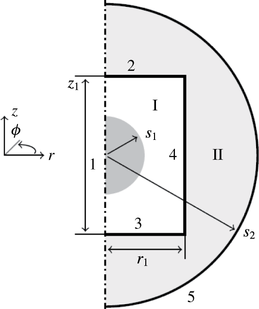
Figure 1. Domain geometry. Arabic and roman numerals denote boundary and domain indexes, respectively. The grey area represents the initial position of the droplet. The symbols $s_{1}$ , $s_{2}$ , $r_{1}$ and $z_{1}$ denote the initial droplet radius, radius of the grounded electrode, radius of the circular electrodes and spacing between the circular electrodes.

2.2 Governing equation and the main assumptions

Because both liquids in domain I are incompressible and Newtonian, the velocity and pressure fields are described by the Navier–Stokes and continuity equations

where the symbols $\unicode[STIX]{x1D70C}$ , $\unicode[STIX]{x1D707}$ , $t$ , $p$ and $\boldsymbol{v}$ denote the liquid density, liquid dynamical viscosity, time, pressure and velocity vector, respectively. The symbols $\boldsymbol{f}_{e}$ , $\boldsymbol{f}_{s}$ and $\boldsymbol{f}_{g}$ represent volume forces in the system.

The inertial term in the Navier–Stokes equations is considered because the values of the Reynolds number ( $Re$ ) in experiments reported in Beranek et al. (Reference Beranek, Flittner, Hrobar, Ethgen and Pribyl2014) were typically higher than 10. In such cases, the inertial forces in the fluid bulk dominate the viscous forces. As will be shown in § 3.1, our simulations predict $Re>100$ in some regimes.

The electric volume force $\boldsymbol{f}_{e}$ can be expressed as either the divergence of the Maxwell stress tensor (Saville Reference Saville1997) or the Korteweg–Helmholtz force density (Grodzinsky Reference Grodzinsky2011), which reads

where $\unicode[STIX]{x1D716}$ and $\unicode[STIX]{x1D714}$ are the fluid permittivity and volume density of free electric charge. The first term on the right-hand side of (2.3) is called the electrostriction force density and is typically lumped with the pressure gradient in (2.1), which leads to a modified definition of pressure (Saville Reference Saville1997). Hence this term was not included in our study. The second and third terms come from the interactions between electric field and dipoles and between electric field and free charges, respectively. The dipole term is important in many electrohydrodynamics problems such as dielectrophoresis or droplet breakup. However, the mechanism of rhythmic droplet motion between two parallel electrodes is mainly driven by the interaction of injected free charge and imposed electric field (Jung et al. Reference Jung, Oh and Kang2008; Jalaal et al. Reference Jalaal, Khorshidi and Esmaeilzadeh2010; Im et al. Reference Im, Noh, Moon and Kang2011). If the droplet will not be in the proximity of an electrode, the net dielectric force will be close to zero and will not significantly contribute to the droplet forcing. For that reason, only the term containing free electric charge is considered in our simulations.

The formulation of the surface tension force in the form of divergence of the capillary pressure tensor $\boldsymbol{f}_{s}$ was adopted from Lafaurie et al. (Reference Lafaurie, Nardone, Scardovelli, Zaleski and Zanetti1994):

where $\boldsymbol{I}$ , $\boldsymbol{n}$ , $\unicode[STIX]{x1D6FE}$ and $\unicode[STIX]{x1D6FF}$ are the unit tensor, normal vector to the liquid–liquid interface, interfacial tension and Dirac delta function (further defined in § 2.4), respectively.

The gravity volume force $\boldsymbol{f}_{g}$ is not involved in the Navier–Stokes equation due to the typically horizontal orientation of the microfluidic devices. In physical experiments with parallel plate electrodes, e.g. Im et al. (Reference Im, Noh, Moon and Kang2011), a highly viscous organic phase is used as well as large electrodes and an organic phase with density similar to that of water. All these measures suppress the effect of the gravity force.

The liquid–liquid interface is tracked by means of the level-set method (Olsson & Kreiss Reference Olsson and Kreiss2005). Local values of the level-set function $\unicode[STIX]{x1D713}$ are calculated from

The symbol $R_{ls}$ represents a stabilizing term of the level-set method that is further discussed in § 2.4. The level-set function $\unicode[STIX]{x1D713}\rightarrow 0$ in the dielectric liquid and $\unicode[STIX]{x1D713}\rightarrow 1$ in the aqueous droplet. Physical properties of the liquids in domain I are then calculated using the level-set function

In electroquasistatic systems (Grodzinsky Reference Grodzinsky2011), the electric field $\boldsymbol{E}$ can be evaluated from

where $\unicode[STIX]{x1D719}$ is the electric potential. The distribution of the electric potential is given by the Gauss law in the form of Poisson’s equation,

Due to the relatively high electrolytic conductivity of the aqueous phase, free electric charge will be collected in a thin EDL at the interface. The characteristic thickness of the EDL is called the Debye length and for a uni-univalent electrolyte (Hrdlicka et al. Reference Hrdlicka, Cervenka, Jindra, Pribyl and Snita2013) it is given by

where $R$ , $T$ , $c$ and $F$ are the molar gas constant, temperature, electrolyte concentration and Faradaic constant, respectively. Depending on the concentration, the Debye length in aqueous system ranges from $1\times 10^{-10}$ to $1\times 10^{-7}$  m. It is difficult to numerically solve dynamical problems where geometrical dimensions are several orders of magnitude larger than the Debye thickness. Pillai et al. (Reference Pillai, Berry, Harvie and Davidson2016) were able to simulate two-phase systems with the ratio of the droplet diameter to the Debye layer thickness equal to 25. The characteristic geometric dimensions of our system are ${\sim}1\times 10^{-3}$  m. Thus the ratio ranges from $1\times 10^{4}$ to $1\times 10^{7}$ . Solution of such problems is nearly impossible even if boundaries are non-moving (Hrdlicka et al. Reference Hrdlicka, Cervenka, Pribyl and Snita2010). Instead we consider that an aqueous droplet is homogeneously charged. The volume concentration of electric charge within the droplet is $\unicode[STIX]{x1D714}_{w}$ . This assumption makes it impossible to simulate jetting or Taylor cone formation. Moreover, the estimation of the dielectric force at the interface (not used in our study because the second right-hand term of (2.3) is neglected) would be imprecise due to a different distribution of the electric field within the droplet. However, it is still efficient to investigate the motion of electrically charged objects in an electric field and to study electrochemical charge injection at the electrodes. The volume density of free electric charge in domain I reads

Other approaches for the treatment of the electric charge distribution in the droplet can be taken into account. For example, the problem can be divided into electric and fluid parts. In the electric part, the electric potential inside the droplet can be set in an iterative manner in order to conserve the surface electric charge of a droplet not attached to an electrode. The obtained field of electric potential can be used in the next integration step to obtain the velocity, pressure and level-set variable distribution. This procedure is extremely time consuming. Moreover, artificial redistribution of the electric charge on the droplet surface will locally violate the velocity field (2.1) and thus also the position of the interface and shape of the droplet. Other problems of this approach originate from the properties of the level-set method. The level-set function is smooth in the spatial domain and the sharpness of the interface is given by the density of finite elements which is, of course, limited. Physical fields (electric potential, velocity, pressure) are represented by the same variables in both phases. The level-set function smoothly switches physical properties such as electric permittivity. So it is difficult and maybe impossible to define the electric potential at an exact coordinate of the interface in each integration step.

As domains I and II are not hydrodynamically coupled, only the distribution of the electric potential is necessary to determine in domain II by the Laplace equation

In principle, it is not necessary to include domain II in the system geometry. However, it significantly helps with stability of the numerical simulations. One can imagine domain II as a cavity filled with air or other dielectric material and surrounded by a grounded Faradaic cage.

We have to consider electric charge balances to describe the electron transfer between the droplet and an electrode. Electrochemical reactions are typically limited by the electrochemical process itself or by mass transport under low or high overpotential (Bard & Faulkner Reference Bard and Faulkner2001; Cervenka et al. Reference Cervenka, Hrdlicka, Pribyl and Snita2012). Because the electric field in experiments with oscillating droplets is typically ${\sim}10^{5}~\text{V}~\text{m}^{-1}$ , a regime limited by mass transport is more probable. We note that under low-intensity electric fields, one has to use Butler–Volmer kinetics or its modification to describe the process (Bard & Faulkner Reference Bard and Faulkner2001). The following charge balance at the electrode–electrolyte interface can then be written

where $V_{d}$ is the droplet volume, $\unicode[STIX]{x1D705}$ is the electrolytic conductivity of the aqueous droplet (alternatively it can be understood as a mass transfer coefficient) and $A$ is the droplet–electrode interfacial area. The electric field strength and electrolytic conductivity are spatially distributed in real aqueous droplets due to possible ionic depletion at the electrode surface under higher overpotential. Because EDL processes are not considered in this study, it is not meaningful to evaluate the distribution of electric conductivity within the droplet. Then a constant $\unicode[STIX]{x1D705}$ is assumed. Another simplification used here is that we replace the local value of $\boldsymbol{n}\boldsymbol{\cdot }\boldsymbol{E}$ by the average electric field strength between the electrodes $\bar{E}$ in (2.12). The average strength is calculated as the difference of electric potential between the electrodes divided by the electrode–electrode distance. Equation (2.12) finally simplifies to the form

The integral of the level-set function over the entire electrode surface represents the electrode–electrolyte interfacial area $A$ . Equation (2.13) uses classical chemical engineering philosophy regarding how to describe a rate $r$ of a complex mass transfer process. Typically $r=k\unicode[STIX]{x0394}XA$ , where $k$ is the mass transfer coefficient, $\unicode[STIX]{x0394}X$ is the driving force and $A$ is the contact area. The driving force, i.e. the gradient of electric potential, is approximated as $\bar{E}$ and can be coupled with the constant $k$ to yield the charging constant (effective mass transfer coefficient) $K$ . The mass transfer coefficient $k$ depends on geometrical parameters (droplet volume) and the effective electrolyte conductivity at the interface. The conductivity at the interface can significantly differ from a bulk value, because the appearance of an ion-depleted zone is highly probable under an intensive electric field (Slouka et al. Reference Slouka, Pribyl, Snita and Postler2007).

2.3 Boundary conditions and initial conditions

Axisymmetric boundary conditions were considered for all quantities at boundary 1; see figure 1. Reference zero electric potential is set at the boundary 5. Wetted wall boundary conditions (Comsol 2013b ) with adjustable contact angle $\unicode[STIX]{x1D703}$ were applied to the boundaries 2, 3 and 4. Reference zero pressure is defined at a single point in domain I. Continuity of electric potential is considered at the boundaries 2, 3 and 4. The other condition at these boundaries results from the application of Gauss’s law (Grodzinsky Reference Grodzinsky2011) and reads

where $\unicode[STIX]{x1D70E}_{s}$ denotes the surface concentration of electric charge and the suffixes are the domain indexes. The dielectric constant in domain II was set to one, i.e. $\unicode[STIX]{x1D716}_{II}=\unicode[STIX]{x1D716}_{0}$ , where $\unicode[STIX]{x1D716}_{0}$ is the vacuum permittivity. Zero surface charge is chosen at boundary 4. The boundaries 2 and 3 are considered to contain the same amount of electric charge $\unicode[STIX]{x1D70E}$ with opposite polarity,

Zero reference pressure and zero velocity were set as the initial conditions in domain I. The phase field function was set to 1 at the position of the aqueous droplet and to 0 elsewhere. The droplet initially did not touch any electrode and the volume charge density was set to an initial value $\unicode[STIX]{x1D714}_{w}=\unicode[STIX]{x1D714}_{0}$ .

2.4 Numerical methods

Comsol Multiphysics 4.4 software (Comsol 2013a ) and the Microfludics module extension (Comsol 2013b ) based on the finite element method were used to solve the axisymmetric problem defined above. The solution was obtained in three steps. The solver internally initialized the level-set function in the first step, equation (2.5). The initial distribution of electric potential was then obtained by solving equations (2.8) and (2.11). Dynamical simulation of the full problem (equations (2.1), (2.2), (2.5), (2.8), (2.11), (2.13)) together with boundary conditions was carried out in the last step.

The Dirac function in (2.4) is approximated by (Comsol 2013b )

The stabilization term $R_{ls}$ in (2.5) reads (Comsol 2013b )

where $a_{1}=1$ m s $^{-1}$ is the reinitialization parameter and $a_{2}$ is the parameter controlling the liquid–liquid interface thickness. The parameter $a_{2}$ was set to one-half of the maximum finite element size.

The multifrontal massively parallel sparse direct solver (Amestoy et al. Reference Amestoy, Duff, Koster and L’Excellent2001) was used for the elimination of large sparse matrixes. The relative tolerance was set to $1\times 10^{-3}$ . A solver based on backward differential formulae of first and second order with automatically adjusted time stepping was used for the time integration of the model equations (Hindmarsh et al. Reference Hindmarsh, Brown, Grant, Lee, Serban, Shumaker and Woodward2005). The relative tolerance of integration steps was set to $1\times 10^{-2}$ .

Spatial domains were discretized with triangular finite elements (figure 2). The mesh consists of approximately $1.7\times 10^{4}$ elements. Most of them are localized in domain I (more than $1.4\times 10^{4}$ ). The distribution of boundary elements is the following: the axis of symmetry (boundary 1, 130 elements), electrodes (boundaries 2 and 3, 51 and 51 elements), solid wall (boundary 4, 102 elements), grounding electrode (boundary 5, 104 elements).

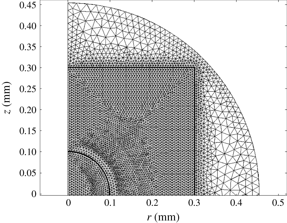
Figure 2. Distribution of triangular elements in one-half of the geometrical domain.

The basic set of values of the dimensional model parameters is summarized in table 1. Values of selected parameters were systematically varied in parametric studies.

2.5 Mesh validation

To characterize the rhythmic motion of the droplet over a longer time period, several normalized characteristics of the system were defined. The normalized volume charge density, droplet–electrode contact area and droplet position read

The volume charge density $\tilde{\unicode[STIX]{x1D714}}\in \left[-1,1\right]$ is normalized by the maximal absolute value of volume charge density in the regular periodic regime. The contact area is normalized by the enclosed area of a circle with a radius of $s_{1}$ . The droplet position is calculated as the mean integral value of the droplet position in domain I normalized by one-half of the electrode distance.

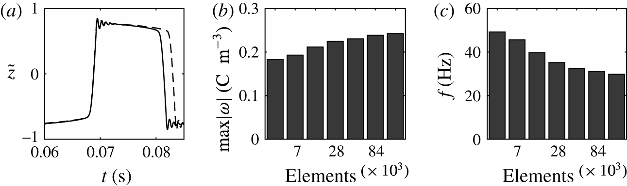
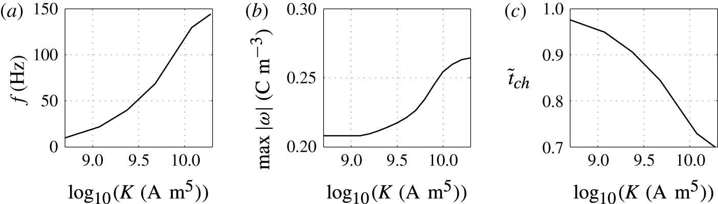
Figure 3. (a) Dependence of the normalized droplet position on time calculated with meshes consisting of 14 106 (solid line) and 28 212 (dashed line) elements in domain I. Effect of the number of mesh elements on the charge acquired by droplet (b) and on the frequency of droplet oscillations (c).

Numerical simulations of the model equations were carried out with several meshes of different quality. The corresponding normalized characteristics are plotted in figure 3. The dependences of the mean droplet position on time for the meshes with $1.4\times 10^{4}$ and $2.8\times 10^{4}$ elements are shown in figure 3(a). The dynamics of droplet transition from one electrode to the other is almost identical. The wavy parts of these time courses are also identical and correspond to damped droplet deformations that appear after touching the electrode. However, the durations of the droplet–electrode contact, i.e. the durations of electrochemical charging, differ by approximately 10 %. This results in slightly higher concentrations of free charge in the droplet (figure 3 b) and a decreased frequency (figure 3 c) in simulations with finer meshes. The time of droplet–electrode contact is affected by the sharpness of the liquid–liquid interface, which is always greater for a finer mesh. The droplet–electrode contact area and charge transfer are then also influenced. Because the mesh test revealed that the qualitative behaviour of the system does not depend on the mesh density and the quantitative characteristics do not differ by more than 15 % for the meshes with $1.4\times 10^{4}$ and $5.6\times 10^{4}$ elements, we decided to use the sparser mesh in our parametric studies. One simulation of 0.25 s time period with the mesh consisting of $1.4\times 10^{4}$ elements typically took only 14 h on 4-core Intel i7-4790 3.6 GHz processors. We further repeated the simulation plotted in figure 3 for $8.4\times 10^{4}$ and $1.12\times 10^{5}$ finite elements. The simulation with $1.12\times 10^{5}$ elements takes more than 10 days of computational time. The numerical solver uses second-order elements to approximate the velocity field and electric potential and first-order elements to approximate the pressure field (Comsol 2013b ). The global error of numerical approximation is then directly proportional to the element size $({\sim}h^{1})$ and convergence is rather gradual. However, the memory demands of the solver grow with ${\sim}h^{-2}$ . The mesh consisting of $1.4\times 10^{4}$ elements thus represents a good compromise between the precision of the numerical approximation and the time demands of the simulations.

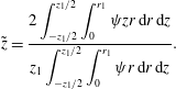
Figure 4. Snapshots of a oscillating droplet. (a) Droplet positions expressed as isosurface plots for $\unicode[STIX]{x1D713}=0.5$ . Droplet colour ranges from $\unicode[STIX]{x1D714}=-0.2~\text{C}~\text{m}^{-3}$ (blue) to $\unicode[STIX]{x1D714}=0.2~\text{C}~\text{m}^{-3}$ (red). (b) Relative pressure distribution and velocity field. Colour palette ranges from $p=-10$  Pa (blue) to $p=1.2$ kPa (red). White arrows indicate the vector field of velocity. (c) Electric field and electric potential distributions. Colour palette ranges from $\unicode[STIX]{x1D719}=-12$ kV (blue) to $\unicode[STIX]{x1D719}=12$ kV (red). Black lines indicate the streamlines of the electric field.

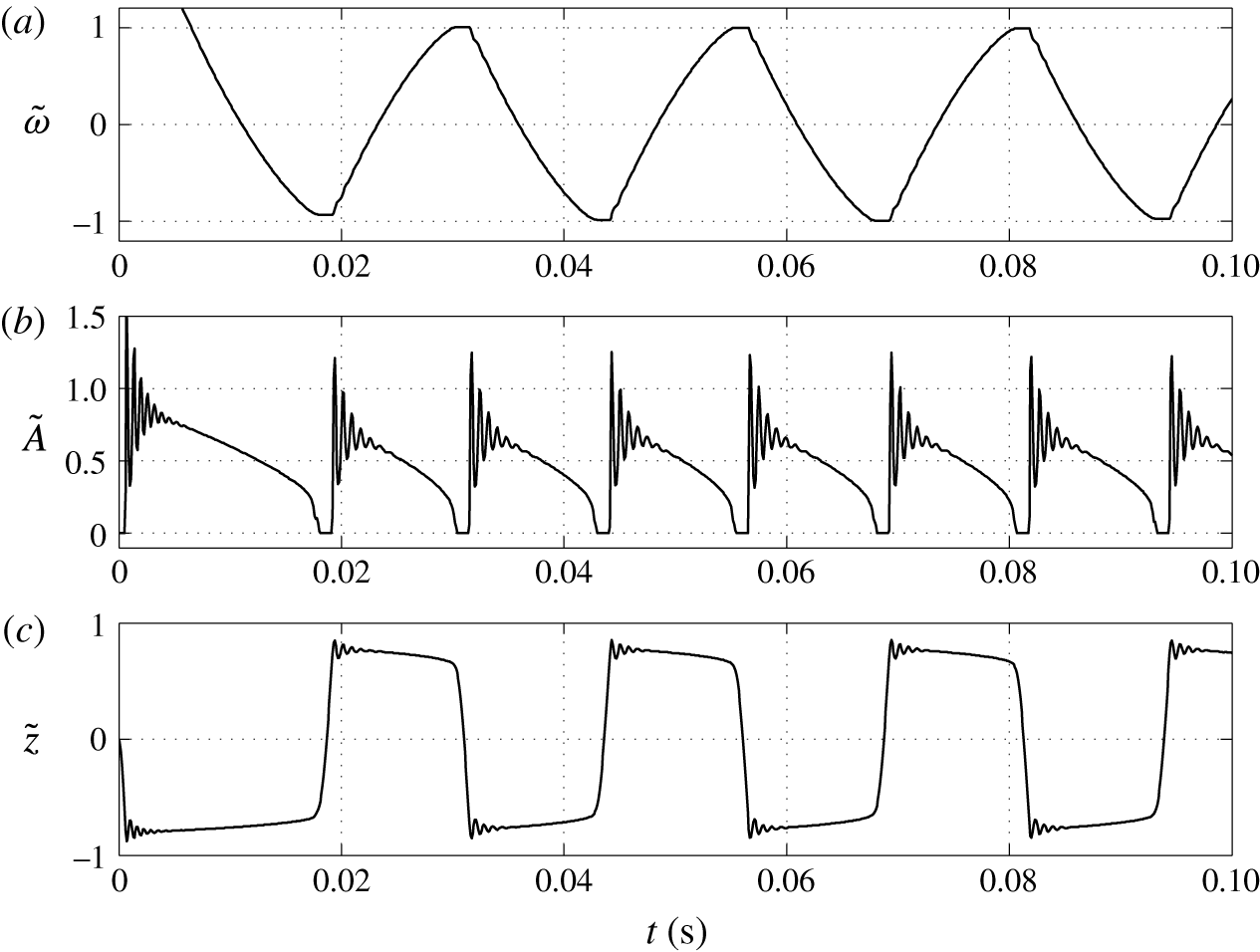
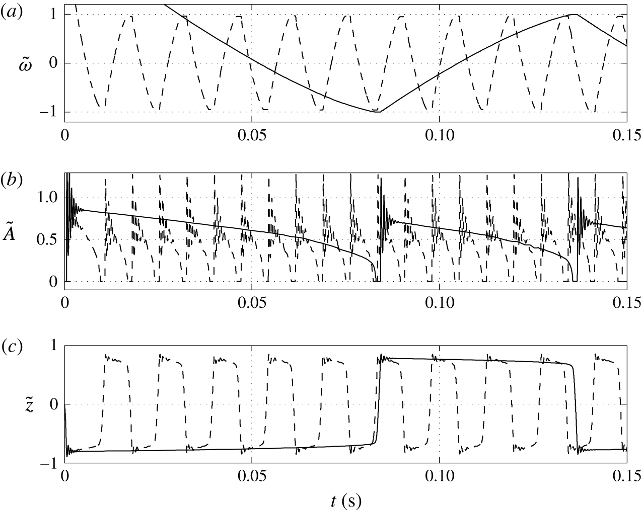
Figure 5. Time dependences of normalized (a) volume charge density, (b) droplet–electrode contact area and (c) droplet position.

3.1 Droplet dynamics and flow pattern

The dynamical behaviour of a charged droplet within a dielectric fluid for the basic set of model parameters is shown in figures 4 and 5 and supplementary movie 1 available at https://doi.org/10.1017/jfm.2017.230. The movie shows the detailed dynamics of droplet deformation and interaction with solid electrodes. One can see that the charged droplet is attracted to the oppositely charged electrode. Once attached, the droplet–electrode interface provides a reaction area for the electrochemical reaction.

The periodic motion of droplets between electrodes consists of a charging phase, where the droplet stays at an electrode, and a non-charging phase, where the droplet moves from one electrode to the other. The charging phase can be accompanied by damped shape oscillations (movie 1) and oscillations of the droplet–electrode contact area and droplet position (figure 5). This behaviour represents a kind of damped harmonic oscillation. Damped oscillators are characterized by a linear or nonlinear damping (friction) term, which is directly proportional to the droplet or object velocity. The van der Pol oscillator represents an oscillator with a nonlinear damping term (van der Pol Reference van der Pol1926). If forced, it can exhibit complex periodic or chaotic behaviour (Parlitz & Lauterborn Reference Parlitz and Lauterborn1987). The damped oscillations of droplet shape appear as a result of energy dissipation due to viscous friction in both liquids at their interface. The radial component of the velocity field is then described by spherical harmonics with a damping function $\exp (-\unicode[STIX]{x1D6FD}t)$ , where $\unicode[STIX]{x1D6FD}$ is the decay factor that can be estimated for different physical situations (Miller & Scriven Reference Miller and Scriven1968).

In relevant experiments (Hase et al. Reference Hase, Watanabe and Yoshikawa2006; Jung et al. Reference Jung, Oh and Kang2008; Im et al. Reference Im, Noh, Moon and Kang2011, Reference Im, Ahn, Yoo, Moon, Lee and Kang2012), only tiny droplet tips mediated the charge transfer across the electrode–droplet interface, which is not in full agreement with the results of our numerical simulations. However, Jalaal et al. (Reference Jalaal, Khorshidi and Esmaeilzadeh2010) observed remarkable droplet deformations in the form of damped oscillations with large contact area at the droplet–electrode interface. The droplet–electrode contact area can be reduced in our simulations, e.g. by setting higher values of the charging constant $K$ or contact angle $\unicode[STIX]{x1D703}$ . Despite higher $K$ or $\unicode[STIX]{x1D703}$ , the model predictions cannot be in full agreement with experimental observations, because spatially uniform droplet charging is assumed and the dielectrophoretic force neglected; see (2.12).

When the oscillations are completely damped, the interfacial area shrinks because the droplet becomes charged by electric charge of the same polarity as the electrode. At a certain moment, the electric volume force exceeds the force of interfacial tension, and the droplet is released into the dielectric fluid and moves to the other electrode. The elongation of the droplet and tip formation before the release have been observed experimentally (Jung et al. Reference Jung, Oh and Kang2008; Im et al. Reference Im, Noh, Moon and Kang2011, Reference Im, Ahn, Yoo, Moon, Lee and Kang2012).

Damped oscillations of the droplet shape are observed after the release. Inertial forces are mostly responsible for these oscillations because the Reynolds number in this particular regime is approximately 120, which is quite far from the Stokes regime ( $Re\ll 1$ ). Here $Re$ is evaluated as $Re=2\bar{v}_{z}s_{1}\unicode[STIX]{x1D70C}_{w}/\unicode[STIX]{x1D702}_{w}$ , where the average axial velocity, $\bar{v}_{z}\approx 0.6~\text{m}~\text{s}^{-1}$ , is estimated as the electrode spacing $z_{1}$ divided by the duration of droplet shift between the electrodes. Similar shape deformations were observed experimentally (Beranek et al. Reference Beranek, Flittner, Hrobar, Ethgen and Pribyl2014).

We note that a Reynolds number significantly higher than 1 is not a very common situation in microfluidics. Typical applications of droplet microfluidics such as slug flow separators or microreactors are accompanied by Stokes flow ( $Re<1$ ). However, in our own experiments (Beranek et al. Reference Beranek, Flittner, Hrobar, Ethgen and Pribyl2014) $Re$ ranged from 10 to 60, which is a result of the high frequency of oscillations; $Re=4$ was reported in Jalaal et al. (Reference Jalaal, Khorshidi and Esmaeilzadeh2010) for a more viscous organic phase. When the inertial forces dominate over the viscous forces, the linear Stokes equation cannot be used for the description of the velocity field. However, turbulent instabilities and intermittency typically appear for $Re\sim 10^{3}$ . Thus the description based on the nonlinear Navier–Stokes equation should be satisfactory and the solution should remain axisymmetric.

Several snapshots of domain I preceding and following the contact of a negatively charged droplet with a positively charged electrode are shown in figure 4. A nearly spherical droplet approaches the electrode. The internal pressure within the droplet is higher than that in the dielectric fluid due to the interfacial tension. The velocity field clearly indicates motion of the droplet and the surrounding dielectric liquid. The electric field is significantly deformed and the streamlines preferentially enter the droplet because of high droplet permittivity. Once the droplet touches the electrode, pressure increases due to the force reaction of the fixed electrode. The middle snapshots show the droplet in the phase of maximal deformation that is accompanied by liquid suction behind the droplet and liquid pushing next to the droplet. When the electric charge within the droplet is reversed, the droplet elongates, touching the electrode with a tiny tip. After release, the nearly spherical droplet moves back to the negatively charged electrode.

One can see that an almost regular periodic regime is attained after one charge reversal of the droplet (figure 5). The charging process is symmetric (figure 5 a) due to the same charging constant at both electrodes. In general, the charging dynamics can be asymmetric due to different kinetics of oxidation and reduction reactions (Bard & Faulkner Reference Bard and Faulkner2001) or asymmetric transport of ions with different electrophoretic mobilities (Grodzinsky Reference Grodzinsky2011). Im et al. (Reference Im, Noh, Moon and Kang2011) found that charging at the negative and positive electrodes differs at most by 5 %. The time dependence of the normalized contact area (figure 5 b) is characterized by damped oscillations that emerge immediately after droplet–electrode contact as a consequence of the shape deformation. As shown in figure 5(a), the oscillations do not significantly affect the charging dynamics. Figure 5(b) further reveals that the contact area can be temporarily larger than the largest cross-sectional area of an ideally spherical droplet of the same volume. The normalized droplet position (figure 5 c) indicates that the droplet remains in contact with the electrodes for ${\sim}10$  ms, the duration of droplet shift between the electrodes is ${\sim}1$  ms, and the oscillation frequency is approximately 40 Hz. The frequency of oscillations in experiments typically does not exceed 10 Hz (Hase et al. Reference Hase, Watanabe and Yoshikawa2006; Im et al. Reference Im, Ahn, Yoo, Moon, Lee and Kang2012; Beranek et al. Reference Beranek, Flittner, Hrobar, Ethgen and Pribyl2014). The difference is caused by the very high electric field strength in this particular simulation ( ${\sim}40~\text{kV}~\text{mm}^{-1}$ ). In experiments, the electric field strength is usually below 1  $\text{kV}~\text{mm}^{-1}$ . We will show in our parametric studies that the oscillation frequency decreases with decreasing electric field strength and is sensitive to other model parameters.

3.2 Effect of surface charge density

Figure 6. Time dependences of normalized (a) volume charge density, (b) droplet–electrode contact area and (c) droplet position. Solid line, $\unicode[STIX]{x1D70E}=2~\text{mC}~\text{m}^{-2}$ ; dashed line, $\unicode[STIX]{x1D70E}=6~\text{mC}~\text{m}^{-2}$ .

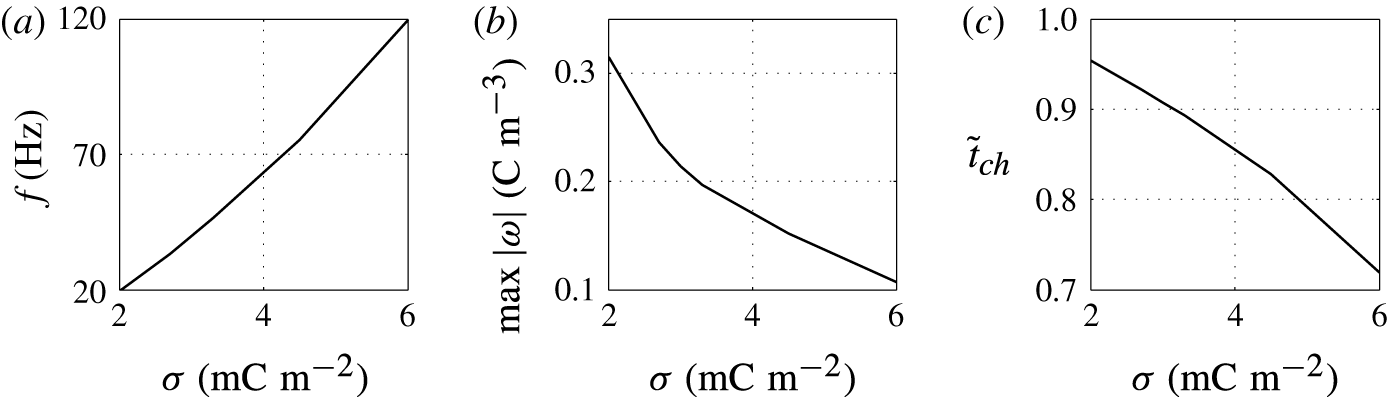
Figure 7. Effects of the surface charge density on (a) frequency of oscillations, (b) charge acquired by droplet and (c) relative time of charging.

The higher the surface charge density on the electrodes, the higher the electric field strength forces the droplet. Monotonic increase of the oscillation frequency with the charge density is observed (figures 6 and 7). This finding is in agreement with available experimental results (Jung et al. Reference Jung, Oh and Kang2008; Im et al. Reference Im, Noh, Moon and Kang2011; Kurimura et al. Reference Kurimura, Ichikawa, Takinoue and Yoshikawa2013; Beranek et al. Reference Beranek, Flittner, Hrobar, Ethgen and Pribyl2014). The dielectric effects, which are neglected in this study, are important only at the electrode surface, where instead of tiny tip formation, the droplet wets the electrode surface. This finally leads to the underestimation of the oscillation frequency because more energy is required for the droplet separation. The electric field strength affects not only the electric volume force acting on the free charge (2.1) but also the kinetics of the electrochemical reactions (2.12). This means that the droplet has to spend less time at a charging electrode to collect enough charge for detachment under a higher electric field strength; see figure 6(c).

In addition to frequency, two other characteristics are plotted in the parametric studies (figure 7). The charge acquired by the droplet, $\max |\unicode[STIX]{x1D714}|$ , is the absolute value of electric charge density acquired within one period of the stable periodic regime, and the relative time of charging, $\tilde{t}_{ch}$ , is the duration of the charging process divided by the period of the stable periodic regime.

The acquired charge decreases with growing surface charge density (figure 7 b). The electric force is the product of the electric field strength and the free charge density. Hence, a lower concentration of free electric charge is necessary to detach the droplet under a higher electric field strength. This finding is meaningful for droplets with relatively large droplet–electrode contact area. In such a case, the electric force required for droplet detachment is given by the droplet–electrode adhesion energy (expressed in the form of the contact angle $\unicode[STIX]{x1D70E}$ ), which is kept constant in this parametric study. However, experiments with rhythmically moving droplets forming only tiny tips during the charging showed that the acquired charge monotonically increases with the electric field strength: $\unicode[STIX]{x1D714}\propto \boldsymbol{E}^{1.33}$ (Jung et al. Reference Jung, Oh and Kang2008) or $\unicode[STIX]{x1D714}\propto \boldsymbol{E}^{1.0}$ (Im et al. Reference Im, Noh, Moon and Kang2011, Reference Im, Ahn, Yoo, Moon, Lee and Kang2012). Because of negligible adhesion energy in the tip-like interaction, the electric charge concentration in a droplet grows with increasing electric field strength as the kinetics of electrochemical charging becomes faster.

The charging process is fast for high surface charge density on the electrode, which leads to a short time of charging and high frequency of droplet oscillations (figure 7 c).

3.3 Effect of charging parameter

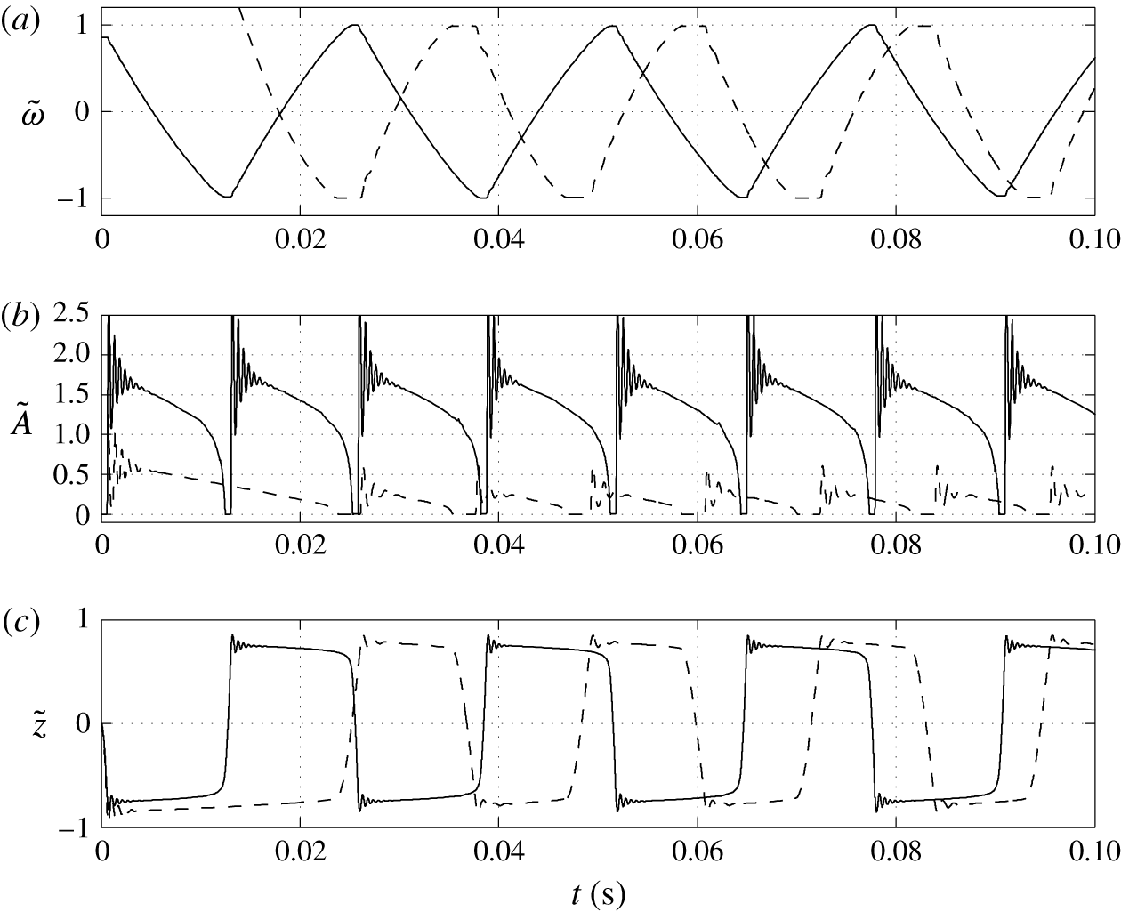
Figure 8. Time dependences of normalized (a) volume charge density, (b) droplet–electrode contact area and (c) droplet position. Solid line, 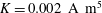$K=0.002~\text{A}~\text{m}^{5}$ ; dashed line, $K=0.02~\text{A}~\text{m}^{5}$ .

Figure 9. Effects of the charging parameter on (a) frequency of oscillations, (b) charge acquired by droplet and (c) relative time of charging.

The imposed electric field affects both the electrochemical kinetics (the charging process) and the electric volume force within the charged fluid. To decouple these two phenomena, it is useful to study the influence of the charging parameter $K$ on rhythmic motion of the droplet. The charging parameter can then be understood as an effective mass transfer coefficient multiplied by the fixed driving force ( $\bar{E}$ ).

Figures 8 and 9 show that the larger the value of $K$ , the higher the oscillation frequency observed. High values of the charging parameter allow for fast droplet charging, significantly reducing the time that the droplet spends at the electrode surface (figure 9 c). Smaller values of $K$ provide an oscillation frequency comparable to that observed in microfluidic experiments (Beranek et al. Reference Beranek, Flittner, Hrobar, Ethgen and Pribyl2014).

In contrast with the results plotted in figure 7(b), the dependence of the acquired charge on the charging parameter is an increasing function (figure 9 b). In this parametric study, the driving force $\bar{E}$ is fixed. A high value of $K$ provides fast charge/mass transfer between the electrodes and droplet. Intensification of charge transfer is also responsible for the same trend observed in Jung et al. (Reference Jung, Oh and Kang2008) and Im et al. (Reference Im, Noh, Moon and Kang2011, Reference Im, Ahn, Yoo, Moon, Lee and Kang2012).

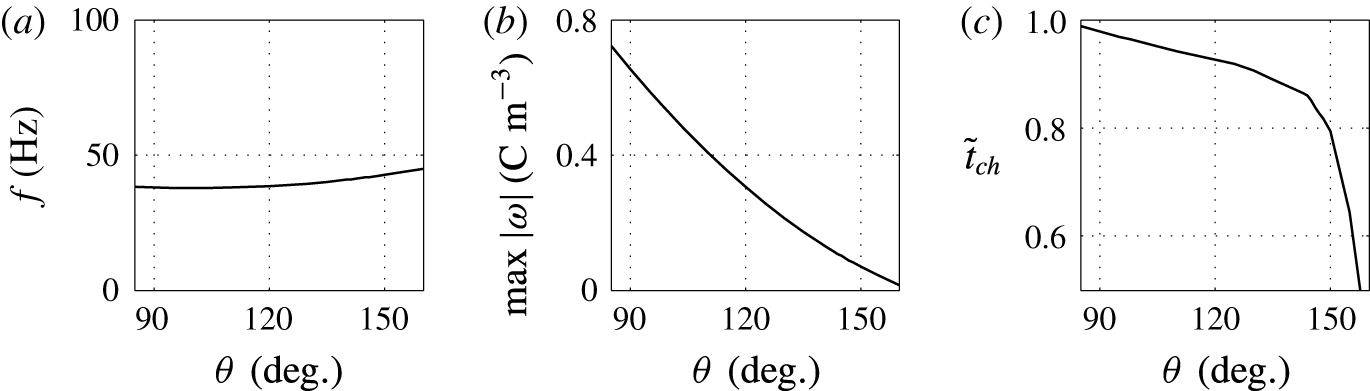
3.4 Effect of contact angle

Figure 10. Time dependences of normalized (a) volume charge density, (b) droplet–electrode contact area and (c) droplet position. Solid line, $\unicode[STIX]{x1D703}=90^{\circ }$ ; dashed line, $\unicode[STIX]{x1D703}=150^{\circ }$ .

Figure 11. Effects of the contact angle on (a) frequency of oscillations, (b) charge acquired by droplet and (c) relative time of charging.

A lower value of the contact angle corresponds to a better wettability of an electrode by the droplet. While the oscillation frequency does not significantly depend on the contact angle, the electrode–droplet contact area remarkably decreases with growing contact angle; see figures 10 and 11. With larger contact area, the adhesion energy barrier increases. This has to be overcome by the electric volume force to detach the droplet. Under constant electric field strength, the force can be provided only by a larger electric charge injected into the droplet. That is the reason why the charging time is slightly longer for $\unicode[STIX]{x1D703}=90^{\circ }$ than for $\unicode[STIX]{x1D703}=150^{\circ }$ (figures 10 c and 11 c). The fact that the acquired electric charge monotonically decreases with the contact angle is demonstrated in figure 11(b).

The results plotted in figures 10 and 11 are physically meaningful, however, experimental studies focused on the contact angle effects in similar experimental system have not been reported.

3.5 Effect of droplet size

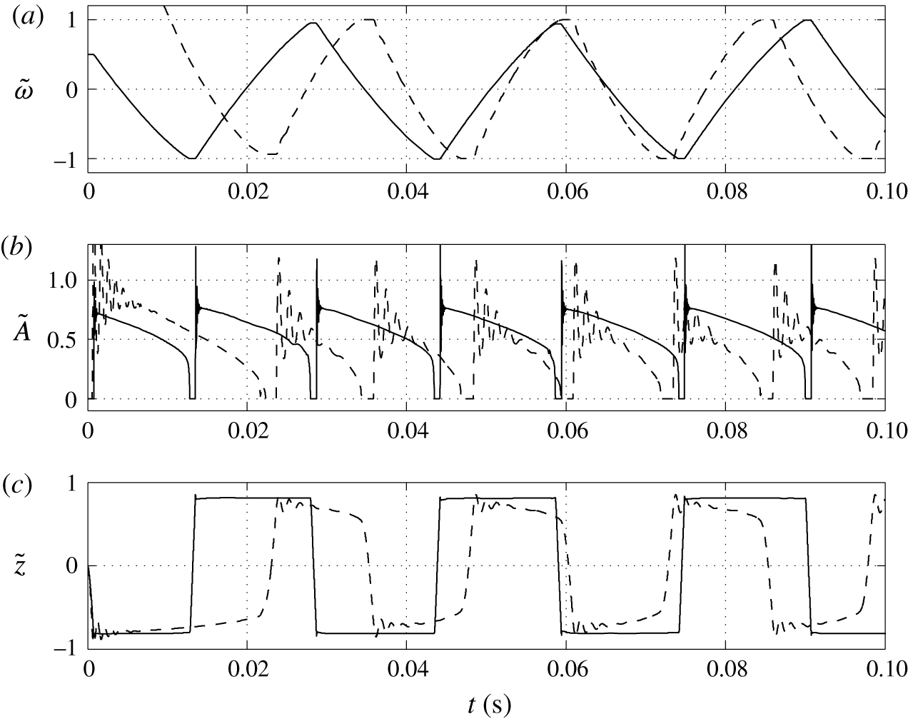
Figure 12. Time dependences of normalized (a) volume charge density, (b) droplet–electrode contact area and (c) droplet position. Solid line, $s_{1}=0.03$ mm; dashed line, $s_{1}=0.14$  mm.

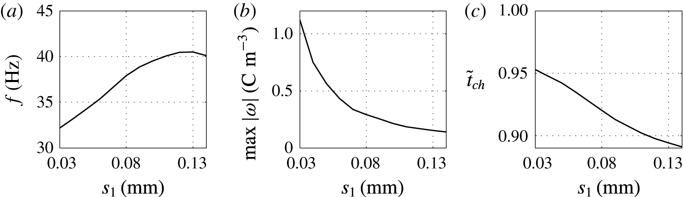
Figure 13. Effects of the droplet radius on (a) frequency of oscillations, (b) charge acquired by droplet and (c) relative time of charging.

Dependences of the velocity of oscillating droplets on the droplet radius were reported in several experimental papers (Jung et al. Reference Jung, Oh and Kang2008; Im et al. Reference Im, Noh, Moon and Kang2011; Kurimura et al. Reference Kurimura, Ichikawa, Takinoue and Yoshikawa2013; Mhatre & Thaokar Reference Mhatre and Thaokar2013). Experiments with a pair of coplanar electrodes (Jung et al. Reference Jung, Oh and Kang2008; Im et al. Reference Im, Noh, Moon and Kang2011), i.e. with geometry most relevant to our theoretical study, reveal that droplet velocity and thus oscillation frequency increases with the droplet radius. Despite the fact that bigger droplets exhibit higher hydrodynamic resistances, they are able to acquire more electric charge, which increases the electric volume force. These observations are in agreement with the results of numerical studies presented here; see figures 12 and 13.

Under a constant electric field, the total amount of acquired electric charge is proportional to the droplet–electrode contact area, equation (2.12), i.e. approximately $\propto s_{1}^{2}$ . Droplet volume $V_{d}\propto s_{1}^{3}$ , hence the electric charge density $\unicode[STIX]{x1D714}\propto s_{1}^{-1}$ . This consideration is in agreement with the hyperbolic-like dependence plotted in figure 13(b).

As the droplet velocity is directly proportional to the total amount of acquired electric charge, the dependence of oscillation frequency on the droplet size should be approximately parabolic, $V_{d}\unicode[STIX]{x1D714}\propto s_{1}^{2}$ . Our simulation revealed the parabolic dependence only for droplets of size less than 0.08 mm (figure 13 a). If the droplet becomes bigger, the frequency increase is slower, then attains a maximum and finally decreases. This nonlinearity appears because friction forces between the droplet and the wall enveloping the two-phase system become important as $s_{1}\rightarrow r_{1}$ .

One feature of smaller droplets when touching an electrode is that there are only a few oscillations of shape. In contrast, large droplets exhibit damped oscillations during the entire period of droplet–electrode interaction (figure 12 b), which is caused by the relatively large inertial forces.

3.6 Effect of permittivity

Figure 14. Time dependences of normalized (a) volume charge density, (b) droplet–electrode contact area and (c) droplet position. Solid line, $\unicode[STIX]{x1D716}_{w}/\unicode[STIX]{x1D716}_{o}=2$ ; dashed line, $\unicode[STIX]{x1D716}_{w}/\unicode[STIX]{x1D716}_{o}=210$ .

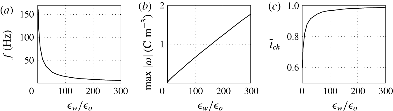
Figure 15. Effects of the permittivity ratio on (a) frequency of oscillations, (b) charge acquired by droplet and (c) relative time of charging.

Finally, the effects of the ratio of droplet to dielectric fluid permittivities $\unicode[STIX]{x1D716}_{w}/\unicode[STIX]{x1D716}_{o}$ on the character of oscillations is examined; see figures 14 and 15. The bigger the ratio, the weaker the electric field present in the charged droplet and the stronger the electric field present in the dielectric fluid. In typical experiments with water droplets dispersed in kerosene, $\unicode[STIX]{x1D716}_{w}/\unicode[STIX]{x1D716}_{o}\approx 27$ . This indicates that the electric field in the droplet is much weaker than in the dielectric fluid. This is valid not only for a homogeneously charged droplet. As a thin EDL is formed in the water phase, the electric field in the droplet bulk will be even weaker.

Figure 14 shows that high $\unicode[STIX]{x1D716}_{w}/\unicode[STIX]{x1D716}_{o}$ can lead to an oscillation frequency below 10 Hz, which is typical for many reported experiments (Hase et al. Reference Hase, Watanabe and Yoshikawa2006; Im et al. Reference Im, Ahn, Yoo, Moon, Lee and Kang2012; Beranek et al. Reference Beranek, Flittner, Hrobar, Ethgen and Pribyl2014). A weaker field in the droplet results in a significant decrease of the oscillation frequency (figure 15 a). A weaker electric field also requires more electric charge to detach the droplet from an electrode (figure 15 b). Hence, the relative time of charging monotonically increases with $\unicode[STIX]{x1D716}_{w}/\unicode[STIX]{x1D716}_{o}$ (figure 15 c).