


1 Introduction
In this paper, Rayleigh–Taylor instability (RTI) induced turbulence between compressible miscible Newtonian fluids is studied. We essentially present a detailed data analysis of a large-scale numerical simulation carried out with a pseudo-spectral code for a strongly stratified initial equilibrium state. By using the full Navier–Stokes equations (NSEs), we have access both to the mixing and to the temperature field and the three Kovásznay modes, namely the vorticity, entropic and acoustic modes, are present.
The RTI is the potentially unstable superposition of a heavy fluid above a lighter one in a slowly variable acceleration field (Rayleigh Reference Rayleigh1883; Taylor Reference Taylor1950). This instability has been the object of continuous interest over the last decades and has been discussed at conferences such as Turbulent Mixing and Beyond and the International Workshop on the Physics of Compressible Turbulent Mixing, as well as in papers such as Anisimov et al. (Reference Anisimov, Drake, Gauthier, Meshkov and Abarzhi2013) and Zhou (Reference Zhou2017). RTI is present in various physical situations but it is often met in high energy density physics and in particular in inertial confinement fusion that aims at obtaining thermonuclear ignition by compressing a small pellet filled with deuterium–tritium (Atzeni & Meyer-Ter-Vhen Reference Atzeni and Meyer-Ter-Vhen2004). The RTI plays also a prominent role in supernova explosions in astrophysics (e.g. Wang & Robertson Reference Wang and Robertson1985, Zingale et al.
Reference Zingale, Woosley, Rendleman, Day and Bell2005). In these situations, the RTI mixes the compounds and perturbs the temperature field, which reduces the nuclear reaction efficiency. Such flows are unsteady, non-uniform and compressible. On the other hand, it is well known that compressibility effects have two different origins. The first one, called static compressibility, is due to the variable density of the fluid. In an acceleration field, it results in a stable stratification and leads to finite density-gradient length scales,
 $L_{\unicode[STIX]{x1D70C}H,L}$
, for the heavy (
$L_{\unicode[STIX]{x1D70C}H,L}$
, for the heavy (
 $H$
) and light (
$H$
) and light (
 $L$
) fluids, respectively. The second one, called dynamic – or intrinsic – compressibility, is essentially an effect of the finite speed of sound. For a perfect gas equation of state (EOS), this effect is governed by the adiabatic indices
$L$
) fluids, respectively. The second one, called dynamic – or intrinsic – compressibility, is essentially an effect of the finite speed of sound. For a perfect gas equation of state (EOS), this effect is governed by the adiabatic indices
 $\unicode[STIX]{x1D6FE}_{H,L}$
of the two fluids. The continuous interest in RTI includes an effort toward the understanding of compressibility effects and some steps have already been made.
$\unicode[STIX]{x1D6FE}_{H,L}$
of the two fluids. The continuous interest in RTI includes an effort toward the understanding of compressibility effects and some steps have already been made.
The linear regime of the RTI for compressible ideal fluids has been studied by several authors in various configurations (Plesset & Hsieh Reference Plesset and Hsieh1964; Blake Reference Blake1972; Mathews & Blumenthal Reference Mathews and Blumenthal1977; Baker Reference Baker1983; Zhou Reference Zhou2017). Stabilizing and destabilizing compressibility effects have been found, but Livescu (Reference Livescu2004) has reconciled these results. Indeed, he has shown that as the equilibrium pressure at the interface increases, the compressibility decreases and the growth rate increases, while as the specific heat ratio increases the compressibility also decreases and the growth rate decreases. Lafay, Le Creurer & Gauthier (Reference Lafay, Le Creurer and Gauthier2007) numerically solve the linear RTI problem for two miscible compressible Newtonian fluids. Diffusions (viscosity, thermal conduction and species diffusion) introduce a cutoff wavenumber beyond which the flow is marginally stable. They confirm that for increasing values of the stratification (attached to the hydrostatic equilibrium), the flow is stabilized, whereas for increasing values of the compressibility parameters (the
 $\unicode[STIX]{x1D6FE}$
values, attached to the fluids), the flow is destabilized.
$\unicode[STIX]{x1D6FE}$
values, attached to the fluids), the flow is destabilized.
In the nonlinear regime, very few works have been devoted to the fully compressible RTI, although a large number of the RTI simulations have been carried out with the Euler equations. These simulations use the limit of small velocities, with a weak initial stratification, i.e. in a quasi-incompressible regime. Moreover, dissipation comes from the dissipation of the numerical scheme.
One of the first contributions to such a RT compressible configuration is due to Wang & Robertson (Reference Wang and Robertson1985), who studied models of accreting X-ray sources in neutron stars. They consider two similar media with a temperature jump, without and with a magnetic field. The mixing process is studied both for single-mode and random-amplitude perturbations and implications for astrophysics are discussed. Later Jin et al. (Reference Jin, Liu, Lu, Cheng, Glimm and Sharp2005) carried out two-dimensional RTI simulations in the deeply compressible regime with the Euler equations and they observed that density stratification is the leading compressibility effect. George & Glimm (Reference George and Glimm2005) established a renormalized self-similar scaling law in this regime. They claim that the time-dependent Atwood number (the dimensionless difference of the heavy and light fluid densities), largely removes the effects of the length scale introduced by compressibility and that self-similarity is maintained in RT multi-mode simulations. Mellado, Sarkar & Zhou (Reference Mellado, Sarkar and Zhou2005) use large-eddy simulation techniques to study compressible RTI with miscible fluids (the mesh sizes were
 $128^{2}\times 256$
and
$128^{2}\times 256$
and
 $256^{2}\times 512$
) and they focus on intrinsic compressibility, that is measured by a Mach number, based on the turbulent velocity fluctuations. Three configurations are considered, where each layer are buoyancy stable, neutral and unstable. They have shown with an energy analysis that the turbulent Mach number has an upper bound. This upper bound may be small enough to limit the RTI-intrinsic compressibility effects. They have also found that potential energy feeds the vertical velocity fluctuations and the transfer to horizontal components is carried out by the pressure–strain terms. Zingale et al. (Reference Zingale, Woosley, Rendleman, Day and Bell2005) also carried out three-dimensional numerical simulations of Rayleigh–Taylor unstable flames in type Ia supernovae with a low Mach number hydrodynamics method. They have shown that the turbulence is highly anisotropic on the large scales and more isotropic on the small scales. Two-dimensional single-mode RTI simulations between Newtonian compressible miscible fluids have been carried out with a self-adaptive pseudo-spectral Chebyshev–Fourier multidomain method (Le Creurer & Gauthier Reference Le Creurer and Gauthier2008). These simulations are started from rest and pursued until the return toward mechanical equilibrium of the mixing. Four regimes – linear and weakly nonlinear, nonlinear steady bubble rise, return toward equilibrium and finally an acoustic wave system – can be identified. They have shown that this one-dimensional system of stationary acoustic waves is damped at the correct rate, i.e. by the physical viscosity. Reckinger, Livescu & Vasilyev (Reference Reckinger, Livescu and Vasilyev2012) and Reckinger, Livescu & Vasilyev (Reference Reckinger, Livescu and Vasilyev2016) are developing a project of wavelet-based adaptive numerical method to handle the compressible RTI. Characteristic analysis is used on the hyperbolic part of the full NSEs to handle the boundary conditions to evacuate the acoustic waves. Two-dimensional single-mode RTI simulations have been carried out so far and are analysed. Compressibility effects are discussed with respect to the Mach and the Atwood numbers. Recently, Sengupta et al. (Reference Sengupta, Sengupta, Sharma, Sengupta, Bhole and Shruti2016) carried out two-dimensional DNS of a system of two air masses initially at different temperatures to trace the non-equilibrium thermodynamics and to test the Stokes’ hypothesis. They conclude that alternatives to this hypothesis based on experimental data would be preferable (Ash Reference Ash2017). Simpler models may also be used to deepen our understanding of compressibility effects since carrying out DNSs with the full NSEs is very expensive, although this approach is used in this paper. A systematic derivation of incompressible-type models has been carried out recently (Schneider Reference Schneider2015; Schneider & Gauthier Reference Schneider and Gauthier2015; Gauthier & Schneider Reference Gauthier and Schneider2017). Anelastic, quasi-isobaric, Sandoval and Boussinesq models have been obtained by means of an asymptotic analysis in terms of the Mach number, although heuristic derivations of the Sandoval and Boussinesq models are available (Livescu & Ristorcelli Reference Livescu and Ristorcelli2007; Livescu Reference Livescu2013). In that respect, the Sandoval model (Reference Sandoval1995) has been set-up for unstratified equilibrium states. Since this model describes the mixture of two fluids of different densities, the resulting mixing is of variable density. These variations may be large even at moderate Atwood number. As such it can be used to evaluate variable-density effects. This is an incompressible-type model, i.e. with an algebraic constraint on the velocity divergence, which precludes the propagation of acoustic waves. A large number of numerical simulations have been performed within this model since Cook & Dimotakis (Reference Cook and Dimotakis2001). Some of them have been carried out at large enough Atwood number and analysis reveal compressibility effects.
$256^{2}\times 512$
) and they focus on intrinsic compressibility, that is measured by a Mach number, based on the turbulent velocity fluctuations. Three configurations are considered, where each layer are buoyancy stable, neutral and unstable. They have shown with an energy analysis that the turbulent Mach number has an upper bound. This upper bound may be small enough to limit the RTI-intrinsic compressibility effects. They have also found that potential energy feeds the vertical velocity fluctuations and the transfer to horizontal components is carried out by the pressure–strain terms. Zingale et al. (Reference Zingale, Woosley, Rendleman, Day and Bell2005) also carried out three-dimensional numerical simulations of Rayleigh–Taylor unstable flames in type Ia supernovae with a low Mach number hydrodynamics method. They have shown that the turbulence is highly anisotropic on the large scales and more isotropic on the small scales. Two-dimensional single-mode RTI simulations between Newtonian compressible miscible fluids have been carried out with a self-adaptive pseudo-spectral Chebyshev–Fourier multidomain method (Le Creurer & Gauthier Reference Le Creurer and Gauthier2008). These simulations are started from rest and pursued until the return toward mechanical equilibrium of the mixing. Four regimes – linear and weakly nonlinear, nonlinear steady bubble rise, return toward equilibrium and finally an acoustic wave system – can be identified. They have shown that this one-dimensional system of stationary acoustic waves is damped at the correct rate, i.e. by the physical viscosity. Reckinger, Livescu & Vasilyev (Reference Reckinger, Livescu and Vasilyev2012) and Reckinger, Livescu & Vasilyev (Reference Reckinger, Livescu and Vasilyev2016) are developing a project of wavelet-based adaptive numerical method to handle the compressible RTI. Characteristic analysis is used on the hyperbolic part of the full NSEs to handle the boundary conditions to evacuate the acoustic waves. Two-dimensional single-mode RTI simulations have been carried out so far and are analysed. Compressibility effects are discussed with respect to the Mach and the Atwood numbers. Recently, Sengupta et al. (Reference Sengupta, Sengupta, Sharma, Sengupta, Bhole and Shruti2016) carried out two-dimensional DNS of a system of two air masses initially at different temperatures to trace the non-equilibrium thermodynamics and to test the Stokes’ hypothesis. They conclude that alternatives to this hypothesis based on experimental data would be preferable (Ash Reference Ash2017). Simpler models may also be used to deepen our understanding of compressibility effects since carrying out DNSs with the full NSEs is very expensive, although this approach is used in this paper. A systematic derivation of incompressible-type models has been carried out recently (Schneider Reference Schneider2015; Schneider & Gauthier Reference Schneider and Gauthier2015; Gauthier & Schneider Reference Gauthier and Schneider2017). Anelastic, quasi-isobaric, Sandoval and Boussinesq models have been obtained by means of an asymptotic analysis in terms of the Mach number, although heuristic derivations of the Sandoval and Boussinesq models are available (Livescu & Ristorcelli Reference Livescu and Ristorcelli2007; Livescu Reference Livescu2013). In that respect, the Sandoval model (Reference Sandoval1995) has been set-up for unstratified equilibrium states. Since this model describes the mixture of two fluids of different densities, the resulting mixing is of variable density. These variations may be large even at moderate Atwood number. As such it can be used to evaluate variable-density effects. This is an incompressible-type model, i.e. with an algebraic constraint on the velocity divergence, which precludes the propagation of acoustic waves. A large number of numerical simulations have been performed within this model since Cook & Dimotakis (Reference Cook and Dimotakis2001). Some of them have been carried out at large enough Atwood number and analysis reveal compressibility effects.
In this way, Livescu & Ristorcelli (Reference Livescu and Ristorcelli2007) stress the importance of the mass flux, i.e. the correlation
 $\overline{\unicode[STIX]{x1D70C}^{\prime }u_{i}^{\prime }}$
, where
$\overline{\unicode[STIX]{x1D70C}^{\prime }u_{i}^{\prime }}$
, where
 $\unicode[STIX]{x1D70C}^{\prime }$
and
$\unicode[STIX]{x1D70C}^{\prime }$
and
 $u_{i}^{\prime }$
are the density and velocity fluctuations and
$u_{i}^{\prime }$
are the density and velocity fluctuations and
 $\overline{\cdot }$
is the Reynolds average, which will be defined below. Indeed it plays a central role in converting the potential energy to the kinetic energy. The pressure gradient is not hydrostatic, as opposed to the Boussinesq flow. They also notice that the integral length scale does not follow the local length scale
$\overline{\cdot }$
is the Reynolds average, which will be defined below. Indeed it plays a central role in converting the potential energy to the kinetic energy. The pressure gradient is not hydrostatic, as opposed to the Boussinesq flow. They also notice that the integral length scale does not follow the local length scale
 $\ell =k^{3/2}/\unicode[STIX]{x1D700}$
, where
$\ell =k^{3/2}/\unicode[STIX]{x1D700}$
, where
 $k$
and
$k$
and
 $\unicode[STIX]{x1D700}$
are the turbulent kinetic energy and its dissipation rate. This might be a variable density effect, as well. Livescu & Ristorcelli (Reference Livescu and Ristorcelli2008) have shown important differences between variable density and Boussinesq RTI. They first noted that ‘the pure heavy fluid mixes more slowly than the pure light fluid’, as shown by the skew character of the density probability density function (PDF), as opposed to the Boussinesq case. The density vertical derivative PDF is found to be asymmetric at higher Atwood number and the magnitude of the density gradients increases. They use a new measure of the non-Boussinesq effects based on the density-specific volume correlation
$\unicode[STIX]{x1D700}$
are the turbulent kinetic energy and its dissipation rate. This might be a variable density effect, as well. Livescu & Ristorcelli (Reference Livescu and Ristorcelli2008) have shown important differences between variable density and Boussinesq RTI. They first noted that ‘the pure heavy fluid mixes more slowly than the pure light fluid’, as shown by the skew character of the density probability density function (PDF), as opposed to the Boussinesq case. The density vertical derivative PDF is found to be asymmetric at higher Atwood number and the magnitude of the density gradients increases. They use a new measure of the non-Boussinesq effects based on the density-specific volume correlation
 $\overline{\unicode[STIX]{x1D70C}^{\prime }{\mathcal{V}}^{\prime }}$
, which is involved in the momentum equation, where
$\overline{\unicode[STIX]{x1D70C}^{\prime }{\mathcal{V}}^{\prime }}$
, which is involved in the momentum equation, where
 ${\mathcal{V}}^{\prime }$
is the specific volume fluctuation. Livescu et al. (Reference Livescu, Ristorcelli, Gore, Dean, Cabot and Cook2009) and Livescu et al. (Reference Livescu, Ristorcelli, Petersen and Gore2010) have also pointed out several variable-density effects, both on the dynamics and on the mixing. Livescu et al. (Reference Livescu, Ristorcelli, Gore, Dean, Cabot and Cook2009) performed a data analysis of the
${\mathcal{V}}^{\prime }$
is the specific volume fluctuation. Livescu et al. (Reference Livescu, Ristorcelli, Gore, Dean, Cabot and Cook2009) and Livescu et al. (Reference Livescu, Ristorcelli, Petersen and Gore2010) have also pointed out several variable-density effects, both on the dynamics and on the mixing. Livescu et al. (Reference Livescu, Ristorcelli, Gore, Dean, Cabot and Cook2009) performed a data analysis of the
 $3072^{3}$
simulation (Cabot & Cook Reference Cabot and Cook2006) and they focus on variable-density effects. Departures from Boussinesq behaviour are seen at the layer edges where the spike front velocity is larger than the bubble front. Indeed, experimental results show that spikes evolve significantly faster than bubbles when the density ratio is large enough (Youngs Reference Youngs1989). Non-Boussinesq effects manifest in several ways. Livescu et al. (Reference Livescu, Ristorcelli, Petersen and Gore2010) emphasized these departures from Boussinesq behaviour on mixing. It is noted that in variable-density flows, mixing is asymmetrical. Asymmetry of the turbulence kinetic energy, vertical mass flux and specific volume pressure-gradient correlation profiles are also noted, as well as the departure of the mean pressure gradient from the hydrostatic value. Departure of the correlation
$3072^{3}$
simulation (Cabot & Cook Reference Cabot and Cook2006) and they focus on variable-density effects. Departures from Boussinesq behaviour are seen at the layer edges where the spike front velocity is larger than the bubble front. Indeed, experimental results show that spikes evolve significantly faster than bubbles when the density ratio is large enough (Youngs Reference Youngs1989). Non-Boussinesq effects manifest in several ways. Livescu et al. (Reference Livescu, Ristorcelli, Petersen and Gore2010) emphasized these departures from Boussinesq behaviour on mixing. It is noted that in variable-density flows, mixing is asymmetrical. Asymmetry of the turbulence kinetic energy, vertical mass flux and specific volume pressure-gradient correlation profiles are also noted, as well as the departure of the mean pressure gradient from the hydrostatic value. Departure of the correlation
 $\overline{\unicode[STIX]{x1D70C}^{\prime }{\mathcal{V}}^{\prime }}$
from normalized density variance is also observed. It is also shown that the specific volume pressure-gradient correlation
$\overline{\unicode[STIX]{x1D70C}^{\prime }{\mathcal{V}}^{\prime }}$
from normalized density variance is also observed. It is also shown that the specific volume pressure-gradient correlation
 $\overline{{\mathcal{V}}\unicode[STIX]{x2202}_{i}p}$
is the largest term in the mass flux equation.
$\overline{{\mathcal{V}}\unicode[STIX]{x2202}_{i}p}$
is the largest term in the mass flux equation.
An anelastic model has been used for large-scale Chebyshev–Fourier–Fourier DNSs with different values for the compressibility parameters (Atwood number and stratification) (Schneider & Gauthier Reference Schneider and Gauthier2016a ). For intermediate Atwood number values and finite stratification, compressibility effects quickly occur and so does the limit of validity. As a result, only nonlinear behaviours are reached. The influence of the compressibility parameters on the growth rate of the RTI is discussed. A low Atwood number and a mildly stratified configuration allow us to reach a turbulent regime. This anelastic model is actually a low Mach number model that only permits modest stratification of the two pure fluids. Moreover this is also a low Atwood number model. As a result, for stratified configurations at finite Atwood number, the full NSEs have to be used.
As a conclusion of this short survey of our knowledge of compressibility effects in the RTI, it is clear that there is much to learn from the true compressible regime, where the three Kovásznay modes are present. It is the objective of this paper to present a comprehensive analysis of a DNS of RTI between two compressible Newtonian fluids at a Reynolds number equal to
 $Re=6\times 10^{4}$
. These simulation results are also compared with those obtained from a simulation carried out at a lower Reynolds number (
$Re=6\times 10^{4}$
. These simulation results are also compared with those obtained from a simulation carried out at a lower Reynolds number (
 $Re=3\times 10^{4}$
) and at the same Atwood number, on a much coarser grid (Gauthier Reference Gauthier2013). They are also compared with results obtained from a simulation carried out within the Boussinesq approximation at the same Reynolds number,
$Re=3\times 10^{4}$
) and at the same Atwood number, on a much coarser grid (Gauthier Reference Gauthier2013). They are also compared with results obtained from a simulation carried out within the Boussinesq approximation at the same Reynolds number,
 $Re=3\times 10^{4}$
and at a low Atwood number (Schneider & Gauthier Reference Schneider and Gauthier2016c
).
$Re=3\times 10^{4}$
and at a low Atwood number (Schneider & Gauthier Reference Schneider and Gauthier2016c
).
The paper is organized as follows. The physical model is described in § 2. The numerical simulations are defined in § 3 and global results – mean quantity profiles, Reynolds numbers, turbulent kinetic energy, mixing properties, vorticity and spectra – are reported in § 4. The anisotropy is discussed in § 5. Comparison between numerical data and the source terms of the Favre-averaged equations is discussed in § 6. Kovásznay-mode decomposition is performed in § 7. A statistical study is reported in § 8. A short visualization is given in § 9 before summarizing the main results in the conclusion.
2 The physical model for compressible miscible Newtonian fluids
We present in this section the governing equations and the mixing model for two miscible Newtonian fluids. The motion takes place in a three-dimensional domain
 $(L_{x},L_{y},L_{z})$
. The heavy fluid (referenced with the subscript
$(L_{x},L_{y},L_{z})$
. The heavy fluid (referenced with the subscript
 $H$
) is initially located in the upper side of the domain, for
$H$
) is initially located in the upper side of the domain, for
 $0\leqslant z\leqslant z_{t}$
, on top of a light fluid (subscript
$0\leqslant z\leqslant z_{t}$
, on top of a light fluid (subscript
 $L$
) occupying the region
$L$
) occupying the region
 $z_{b}\leqslant z\leqslant 0$
, where
$z_{b}\leqslant z\leqslant 0$
, where
 $z_{b}$
and
$z_{b}$
and
 $z_{t}$
denote the coordinates of the bottom and the top of the domain. The mixing of these two compressible miscible fluids is analysed within the framework of the single fluid approximation. The partial densities,
$z_{t}$
denote the coordinates of the bottom and the top of the domain. The mixing of these two compressible miscible fluids is analysed within the framework of the single fluid approximation. The partial densities,
 $\unicode[STIX]{x1D70C}_{H}$
and
$\unicode[STIX]{x1D70C}_{H}$
and
 $\unicode[STIX]{x1D70C}_{L}$
are defined such that
$\unicode[STIX]{x1D70C}_{L}$
are defined such that
 $\int _{V}\unicode[STIX]{x1D70C}_{H}\,\text{d}x\,\text{d}y\,\text{d}z=m_{H}$
and
$\int _{V}\unicode[STIX]{x1D70C}_{H}\,\text{d}x\,\text{d}y\,\text{d}z=m_{H}$
and
 $\int _{V}\unicode[STIX]{x1D70C}_{L}\,\text{d}x\,\text{d}y\,\text{d}z=m_{L}$
, where
$\int _{V}\unicode[STIX]{x1D70C}_{L}\,\text{d}x\,\text{d}y\,\text{d}z=m_{L}$
, where
 $m_{H,L}$
are the masses of the heavy and light fluids contained in the total volume
$m_{H,L}$
are the masses of the heavy and light fluids contained in the total volume
 $V$
. The ‘partial pressures–partial densities’ mixing model is written
$V$
. The ‘partial pressures–partial densities’ mixing model is written
 $$\begin{eqnarray}p=p_{H}+p_{L}\quad \text{and}\quad \unicode[STIX]{x1D70C}=\unicode[STIX]{x1D70C}_{H}+\unicode[STIX]{x1D70C}_{L}.\end{eqnarray}$$
A fluid concentration,
 $c$
, is also defined such that the partial densities are
$c$
, is also defined such that the partial densities are
 $$\begin{eqnarray}\unicode[STIX]{x1D70C}_{H}=c\unicode[STIX]{x1D70C}\quad \text{and}\quad \unicode[STIX]{x1D70C}_{L}=(1-c)\unicode[STIX]{x1D70C}.\end{eqnarray}$$
Let us recall the full NSEs for a binary mixture of two Newtonian miscible fluids (Hirschfelder, Curtiss & Bird Reference Hirschfelder, Curtiss and Bird1954, chap. 11), (Cook Reference Cook2009)
 $$\begin{eqnarray}\left.\begin{array}{@{}c@{}}\unicode[STIX]{x2202}_{t}\unicode[STIX]{x1D70C}+\unicode[STIX]{x2202}_{j}\unicode[STIX]{x1D70C}u_{j}=0,\\ \unicode[STIX]{x2202}_{t}\unicode[STIX]{x1D70C}u_{i}+\unicode[STIX]{x2202}_{j}\unicode[STIX]{x1D70C}u_{i}u_{j}=-\unicode[STIX]{x2202}_{i}p+\unicode[STIX]{x2202}_{j}\unicode[STIX]{x1D70E}_{ij}-g\unicode[STIX]{x1D70C}\unicode[STIX]{x1D6FF}_{i3},\\ \displaystyle \unicode[STIX]{x2202}_{t}\unicode[STIX]{x1D70C}e+\unicode[STIX]{x2202}_{j}\unicode[STIX]{x1D70C}u_{j}e=-p\unicode[STIX]{x2202}_{i}u_{i}+\unicode[STIX]{x1D70E}_{ij}\unicode[STIX]{x1D634}_{ij}-\unicode[STIX]{x2202}_{i}q_{i},\\ \displaystyle \unicode[STIX]{x2202}_{t}\unicode[STIX]{x1D70C}c+\unicode[STIX]{x2202}_{j}\unicode[STIX]{x1D70C}u_{j}c=\unicode[STIX]{x2202}_{i}[(\unicode[STIX]{x1D70C}{\mathcal{D}})\unicode[STIX]{x2202}_{i}c],\end{array}\right\}\end{eqnarray}$$
where
 $u_{i}$
,
$u_{i}$
,
 $(i=1,2,3)$
, are the three velocity components. The equation of state of each component is
$(i=1,2,3)$
, are the three velocity components. The equation of state of each component is
 $$\begin{eqnarray}p_{\unicode[STIX]{x1D6FC}}=\unicode[STIX]{x1D70C}_{\unicode[STIX]{x1D6FC}}{\mathcal{R}}/{\mathcal{M}}_{\unicode[STIX]{x1D6FC}}T\quad \text{with }\unicode[STIX]{x1D6FC}=H,L.\end{eqnarray}$$
The momentum equation (2.3) contains the buoyancy term
 $-g\unicode[STIX]{x1D70C}\unicode[STIX]{x1D6FF}_{i3}$
, where
$-g\unicode[STIX]{x1D70C}\unicode[STIX]{x1D6FF}_{i3}$
, where
 $g$
is the acceleration due to gravity. The stress tensor,
$g$
is the acceleration due to gravity. The stress tensor,
 $\unicode[STIX]{x1D70E}_{ij}=\unicode[STIX]{x1D707}(\unicode[STIX]{x2202}_{j}u_{i}+\unicode[STIX]{x2202}_{i}u_{j}-2/3\unicode[STIX]{x1D6FF}_{ij}\unicode[STIX]{x2202}_{\ell }u_{\ell })$
, where
$\unicode[STIX]{x1D70E}_{ij}=\unicode[STIX]{x1D707}(\unicode[STIX]{x2202}_{j}u_{i}+\unicode[STIX]{x2202}_{i}u_{j}-2/3\unicode[STIX]{x1D6FF}_{ij}\unicode[STIX]{x2202}_{\ell }u_{\ell })$
, where
 $\unicode[STIX]{x1D707}$
is the dynamic viscosity coefficient, is calculated within the Stokes approximation, and
$\unicode[STIX]{x1D707}$
is the dynamic viscosity coefficient, is calculated within the Stokes approximation, and
 $\unicode[STIX]{x1D634}_{ij}=1/2(\unicode[STIX]{x2202}_{j}u_{i}+\unicode[STIX]{x2202}_{i}u_{j})/2$
is the rate-of-deformation tensor. This is valid for monoatomic gases and consistent with the value
$\unicode[STIX]{x1D634}_{ij}=1/2(\unicode[STIX]{x2202}_{j}u_{i}+\unicode[STIX]{x2202}_{i}u_{j})/2$
is the rate-of-deformation tensor. This is valid for monoatomic gases and consistent with the value
 $\unicode[STIX]{x1D6FE}=5/3$
. The dissipation function in the energy equation is
$\unicode[STIX]{x1D6FE}=5/3$
. The dissipation function in the energy equation is
 $\unicode[STIX]{x1D70E}_{ij}\unicode[STIX]{x1D634}_{ij}$
. The heat flux expression is
$\unicode[STIX]{x1D70E}_{ij}\unicode[STIX]{x1D634}_{ij}$
. The heat flux expression is
 $q_{i}=+h_{\unicode[STIX]{x1D6FC}}J_{\unicode[STIX]{x1D6FC}i}-\unicode[STIX]{x1D705}\unicode[STIX]{x2202}_{i}T$
, (
$q_{i}=+h_{\unicode[STIX]{x1D6FC}}J_{\unicode[STIX]{x1D6FC}i}-\unicode[STIX]{x1D705}\unicode[STIX]{x2202}_{i}T$
, (
 $\unicode[STIX]{x1D6FC}=H,L$
) where
$\unicode[STIX]{x1D6FC}=H,L$
) where
 $h_{\unicode[STIX]{x1D6FC}}$
is the enthalpy of the species
$h_{\unicode[STIX]{x1D6FC}}$
is the enthalpy of the species
 $\unicode[STIX]{x1D6FC}$
and
$\unicode[STIX]{x1D6FC}$
and
 $J_{\unicode[STIX]{x1D6FC}i}=-\unicode[STIX]{x1D70C}{\mathcal{D}}\unicode[STIX]{x2202}_{i}c_{\unicode[STIX]{x1D6FC}}$
is the diffusive mass flux. The diffusion coefficient of species is
$J_{\unicode[STIX]{x1D6FC}i}=-\unicode[STIX]{x1D70C}{\mathcal{D}}\unicode[STIX]{x2202}_{i}c_{\unicode[STIX]{x1D6FC}}$
is the diffusive mass flux. The diffusion coefficient of species is
 ${\mathcal{D}}$
and the thermal conductivity coefficient is denoted
${\mathcal{D}}$
and the thermal conductivity coefficient is denoted
 $\unicode[STIX]{x1D705}$
. The molar weights are
$\unicode[STIX]{x1D705}$
. The molar weights are
 ${\mathcal{M}}_{H}$
and
${\mathcal{M}}_{H}$
and
 ${\mathcal{M}}_{L}$
and the perfect gas constant is
${\mathcal{M}}_{L}$
and the perfect gas constant is
 ${\mathcal{R}}$
. Finally, let us recall that this system contains the three Kovásznay modes, namely the vorticity, entropic and acoustic modes (Chu & Kovásznay Reference Chu and Kovásznay1958), see (Monin & Yaglom Reference Monin and Yaglom1962, § 1.7). System (2.3) is written in a dimensionless form with the following units. The reference of length is the width box,
${\mathcal{R}}$
. Finally, let us recall that this system contains the three Kovásznay modes, namely the vorticity, entropic and acoustic modes (Chu & Kovásznay Reference Chu and Kovásznay1958), see (Monin & Yaglom Reference Monin and Yaglom1962, § 1.7). System (2.3) is written in a dimensionless form with the following units. The reference of length is the width box,
 $L_{y}$
(or
$L_{y}$
(or
 $L_{x}$
). The unit of time is
$L_{x}$
). The unit of time is
 $(L_{y}/g)^{1/2}$
. The unit of mass, denoted
$(L_{y}/g)^{1/2}$
. The unit of mass, denoted
 $\unicode[STIX]{x1D70C}_{r}$
, is given by the half-sum of densities on each side of the pseudo-interface and the temperature reference is given by a uniform temperature, denoted
$\unicode[STIX]{x1D70C}_{r}$
, is given by the half-sum of densities on each side of the pseudo-interface and the temperature reference is given by a uniform temperature, denoted
 $T_{r}$
. As a result, the complete dimensionless NSEs for a binary mixing of Newtonian miscible fluids are written
$T_{r}$
. As a result, the complete dimensionless NSEs for a binary mixing of Newtonian miscible fluids are written
 $$\begin{eqnarray}\left.\begin{array}{@{}c@{}}\unicode[STIX]{x2202}_{t}\unicode[STIX]{x1D70C}+\unicode[STIX]{x2202}_{j}(\unicode[STIX]{x1D70C}u_{j})=0,\\ \unicode[STIX]{x1D70C}(\unicode[STIX]{x2202}_{t}u_{i}+u_{j}\unicode[STIX]{x2202}_{j}u_{i})=-Sr^{-1}\unicode[STIX]{x2202}_{i}p+Re^{-1}\unicode[STIX]{x2202}_{j}\unicode[STIX]{x1D70E}_{ij}-\unicode[STIX]{x1D70C}\unicode[STIX]{x1D6FF}_{i3},\\ \displaystyle \unicode[STIX]{x1D70C}C_{v;m}(\unicode[STIX]{x2202}_{t}T+u_{j}\unicode[STIX]{x2202}_{j}T)=(\unicode[STIX]{x1D6FE}_{r}-1)[SrRe^{-1}\unicode[STIX]{x1D70E}_{ij}\unicode[STIX]{x1D634}_{ij}-p\unicode[STIX]{x2202}_{j}u_{j}]\\ -Re^{-1}Sc^{-1}Td_{c}C_{v;m}\unicode[STIX]{x2202}_{jj}c+\,Re^{-1}Pr^{-1}\unicode[STIX]{x0394}_{H,L}^{\star }\unicode[STIX]{x2202}_{i}[T\unicode[STIX]{x2202}_{i}c]\\ +Re^{-1}Pr^{-1}\unicode[STIX]{x1D6FE}_{r}\unicode[STIX]{x2202}_{jj}T,\\ \displaystyle \unicode[STIX]{x2202}_{t}c+u_{j}\unicode[STIX]{x2202}_{j}c=(\unicode[STIX]{x1D70C}ReSc)^{-1}\unicode[STIX]{x2202}_{jj}c,\\ p=\unicode[STIX]{x1D70C}T(1+A_{t}-2A_{t}c).\end{array}\right\}\end{eqnarray}$$
The specific heats at constant volume and pressure of each fluid and their ratios are denoted
 $C_{v,p;H,L}$
and
$C_{v,p;H,L}$
and
 $\unicode[STIX]{x1D6FE}_{H,L}$
. The mixing adiabatic index is
$\unicode[STIX]{x1D6FE}_{H,L}$
. The mixing adiabatic index is
 $\unicode[STIX]{x1D6FE}_{m}(c)=C_{p,m}/C_{v,m}$
, where the expression of the mixture-specific heats read
$\unicode[STIX]{x1D6FE}_{m}(c)=C_{p,m}/C_{v,m}$
, where the expression of the mixture-specific heats read
 $C_{v,p;m}(c)=cC_{v,p;H}+(1-c)C_{v,p;L}$
. The reference concentration is chosen to be
$C_{v,p;m}(c)=cC_{v,p;H}+(1-c)C_{v,p;L}$
. The reference concentration is chosen to be
 $c_{ref}=(1-A_{t})/2$
, where
$c_{ref}=(1-A_{t})/2$
, where
 $A_{t}=(\unicode[STIX]{x1D70C}_{H}-\unicode[STIX]{x1D70C}_{L})/(\unicode[STIX]{x1D70C}_{H}+\unicode[STIX]{x1D70C}_{L})$
is the Atwood number. We also use the reference value
$A_{t}=(\unicode[STIX]{x1D70C}_{H}-\unicode[STIX]{x1D70C}_{L})/(\unicode[STIX]{x1D70C}_{H}+\unicode[STIX]{x1D70C}_{L})$
is the Atwood number. We also use the reference value
 $\unicode[STIX]{x1D6FE}_{r}=\unicode[STIX]{x1D6FE}_{m}(c_{ref})$
. The derivative with respect to the concentration is denoted
$\unicode[STIX]{x1D6FE}_{r}=\unicode[STIX]{x1D6FE}_{m}(c_{ref})$
. The derivative with respect to the concentration is denoted
 $d_{c}$
and the dimensionless difference of specific heats at constant pressure is
$d_{c}$
and the dimensionless difference of specific heats at constant pressure is
 $\unicode[STIX]{x1D6E5}_{H,L}^{\star }$
(see appendix A). The expression of the stratification parameter and the Reynolds, Schmidt and Prandtl numbers are
$\unicode[STIX]{x1D6E5}_{H,L}^{\star }$
(see appendix A). The expression of the stratification parameter and the Reynolds, Schmidt and Prandtl numbers are
 $$\begin{eqnarray}Sr=\frac{gL_{y}}{{\mathcal{R}}T/{\mathcal{M}}_{r}},\quad Re=\frac{g^{1/2}L_{y}^{3/2}}{\unicode[STIX]{x1D707}/\unicode[STIX]{x1D70C}_{r}},\quad Sc=\frac{\unicode[STIX]{x1D707}}{\unicode[STIX]{x1D70C}D}\quad \text{and}\quad Pr=\unicode[STIX]{x1D6FE}_{r}\frac{\unicode[STIX]{x1D707}C_{v,ref}}{\unicode[STIX]{x1D705}},\end{eqnarray}$$
where
 $2/{\mathcal{M}}_{r}=1/{\mathcal{M}}_{H}+1/{\mathcal{M}}_{L}$
and
$2/{\mathcal{M}}_{r}=1/{\mathcal{M}}_{H}+1/{\mathcal{M}}_{L}$
and
 $C_{v,ref}=C_{v;m}(c_{ref})$
is the reference value. System of PDEs (2.3) has to be equipped with appropriate initial and boundary conditions. In physical situations, e.g. in astrophysical configurations or in a small pellet in inertial confinement fusion, the boundaries of the computational domain used here are actually contact surfaces between the fluids. As a result, acoustic waves are partially reflected or transmitted through these contact surfaces. A limit case is studied here where acoustic waves are reflected and remain inside the domain. The opposite limit case where acoustic waves are fully transmitted is also possible (Reckinger et al.
Reference Reckinger, Livescu and Vasilyev2016). In any case, the number of boundary conditions that has to be specified is given by the analysis of Strikwerda (Reference Strikwerda1977). The numerical implementation may be achieved by using the approach proposed by Thompson (Reference Thompson1990) and it has been applied in a spectral framework by Boudesocque-Dubois et al. (Reference Boudesocque-Dubois, Clarisse and Gauthier2003), among others. As a result, we chose periodic boundary conditions in the horizontal
$C_{v,ref}=C_{v;m}(c_{ref})$
is the reference value. System of PDEs (2.3) has to be equipped with appropriate initial and boundary conditions. In physical situations, e.g. in astrophysical configurations or in a small pellet in inertial confinement fusion, the boundaries of the computational domain used here are actually contact surfaces between the fluids. As a result, acoustic waves are partially reflected or transmitted through these contact surfaces. A limit case is studied here where acoustic waves are reflected and remain inside the domain. The opposite limit case where acoustic waves are fully transmitted is also possible (Reckinger et al.
Reference Reckinger, Livescu and Vasilyev2016). In any case, the number of boundary conditions that has to be specified is given by the analysis of Strikwerda (Reference Strikwerda1977). The numerical implementation may be achieved by using the approach proposed by Thompson (Reference Thompson1990) and it has been applied in a spectral framework by Boudesocque-Dubois et al. (Reference Boudesocque-Dubois, Clarisse and Gauthier2003), among others. As a result, we chose periodic boundary conditions in the horizontal
 $(x,y)$
-directions for all physical quantities with stress-free conditions along the top and bottom boundaries for the velocity. There is no flow and therefore no mass flux through the top and bottom boundaries. The temperature is kept fixed at the bottom boundary and there is no heat flux at the top. These boundary conditions are written
$(x,y)$
-directions for all physical quantities with stress-free conditions along the top and bottom boundaries for the velocity. There is no flow and therefore no mass flux through the top and bottom boundaries. The temperature is kept fixed at the bottom boundary and there is no heat flux at the top. These boundary conditions are written
 $$\begin{eqnarray}\left.\begin{array}{@{}c@{}}\unicode[STIX]{x2202}_{z}u_{x,y}(x,y,z=z_{b},z_{t};t)=u_{z}(x,y,z=z_{b},z_{t};t)=0,\\ \unicode[STIX]{x2202}_{z}c(x,y,z=z_{b},z_{t};t)=0,\\ T(x,y,z=z_{b};t)=1\quad \text{and}\quad \unicode[STIX]{x2202}_{z}T(x,y,z=z_{t};t)=0.\end{array}\right\}\end{eqnarray}$$
There is no boundary condition on the density and pressure.
2.1 The averaging procedures
For the data analysis in the turbulent regime we will use either the Reynolds (
 $\overline{\cdot }$
) or the Favre (
$\overline{\cdot }$
) or the Favre (
 $\widetilde{\cdot }$
) averaging procedure. Since the turbulent mixing layer is homogeneous in the two horizontal directions, the ensemble mean of a variable
$\widetilde{\cdot }$
) averaging procedure. Since the turbulent mixing layer is homogeneous in the two horizontal directions, the ensemble mean of a variable
 $\unicode[STIX]{x1D711}$
is computed from a spatial average as
$\unicode[STIX]{x1D711}$
is computed from a spatial average as
 $$\begin{eqnarray}\unicode[STIX]{x1D711}(x,y,z,t)=\overline{\unicode[STIX]{x1D711}}(z,t)+\unicode[STIX]{x1D711}^{\prime }(x,y,z,t),\end{eqnarray}$$
where
 $\overline{\unicode[STIX]{x1D711}}(z,t)=(L_{x}L_{y})^{-1}\int \unicode[STIX]{x1D711}(x,y,z,t)\,\text{d}x\,\text{d}y$
. We will also use the volume average over a fraction of the mixing layer defined as
$\overline{\unicode[STIX]{x1D711}}(z,t)=(L_{x}L_{y})^{-1}\int \unicode[STIX]{x1D711}(x,y,z,t)\,\text{d}x\,\text{d}y$
. We will also use the volume average over a fraction of the mixing layer defined as
 $$\begin{eqnarray}\langle \overline{\unicode[STIX]{x1D711}}\rangle _{\unicode[STIX]{x1D6FD}}(t)=\frac{1}{\unicode[STIX]{x1D6FD}h(t)}\int _{-\unicode[STIX]{x1D6FD}h_{L}(t)}^{\unicode[STIX]{x1D6FD}h_{H}(t)}\overline{\unicode[STIX]{x1D711}}(z,t)\,\text{d}z,\end{eqnarray}$$
where
 $\unicode[STIX]{x1D6FD}$
is such that
$\unicode[STIX]{x1D6FD}$
is such that
 $0<\unicode[STIX]{x1D6FD}\leqslant 1$
. For density-variable flows, the Favre averaging is defined as
$0<\unicode[STIX]{x1D6FD}\leqslant 1$
. For density-variable flows, the Favre averaging is defined as
 $$\begin{eqnarray}\unicode[STIX]{x1D711}=\unicode[STIX]{x1D711}^{\prime \prime }+\widetilde{\unicode[STIX]{x1D711}}\quad \text{with }\widetilde{\unicode[STIX]{x1D711}}=\frac{\overline{\unicode[STIX]{x1D70C}\unicode[STIX]{x1D711}}}{\overline{\unicode[STIX]{x1D70C}}},\end{eqnarray}$$
for any quantity
 $\unicode[STIX]{x1D711}$
but the density and the pressure.
$\unicode[STIX]{x1D711}$
but the density and the pressure.
Table 1. List of parameter values used in the three simulations. The specific heat ratios of the two fluids are equal,
 $\unicode[STIX]{x1D6FE}_{H}=\unicode[STIX]{x1D6FE}_{L}=\unicode[STIX]{x1D6FE}_{r}=5/3$
.
$\unicode[STIX]{x1D6FE}_{H}=\unicode[STIX]{x1D6FE}_{L}=\unicode[STIX]{x1D6FE}_{r}=5/3$
.

Table 2. Characteristics of the numerical simulation
 $Sr6\text{-}Re6\times 10^{4}$
: the Atwood number, the stratification, the Reynolds number, the speeds of sound in the heavy (
$Sr6\text{-}Re6\times 10^{4}$
: the Atwood number, the stratification, the Reynolds number, the speeds of sound in the heavy (
 $H$
) and light (
$H$
) and light (
 $L$
) fluids, the density-gradient length scales and the ratios of the densities and pressures between the top and the bottom of the domain.
$L$
) fluids, the density-gradient length scales and the ratios of the densities and pressures between the top and the bottom of the domain.
3 Numerical simulations
3.1 Simulation definition
The system of PDEs (2.5) is solved in the code Aménophis, and those features are recalled in appendix B. The characteristics of the simulations under study are summarized in tables 1 and 2. The
 $Sr6\text{-}Re3\times 10^{4}$
spatial resolution is
$Sr6\text{-}Re3\times 10^{4}$
spatial resolution is
 $(6\times 64)\times 382^{2}\approx 56M$
. The
$(6\times 64)\times 382^{2}\approx 56M$
. The
 $Sr6\text{-}Re6\times 10^{4}$
simulation is started with
$Sr6\text{-}Re6\times 10^{4}$
simulation is started with
 $(9\times 64)\times 576^{2}\approx 191M$
collocation points. It is increased up to
$(9\times 64)\times 576^{2}\approx 191M$
collocation points. It is increased up to
 $(9\times 100)\times 1000^{2}=900M$
and later decreased at
$(9\times 100)\times 1000^{2}=900M$
and later decreased at
 $(9\times 64)\times 640^{2}\approx 236M$
collocation points. The grid modifications are achieved in the spectral space such as described in Schneider et al. (Reference Schneider, Hammouch, Labrosse and Gauthier2015, § 3.8) and recalled in appendix B. The
$(9\times 64)\times 640^{2}\approx 236M$
collocation points. The grid modifications are achieved in the spectral space such as described in Schneider et al. (Reference Schneider, Hammouch, Labrosse and Gauthier2015, § 3.8) and recalled in appendix B. The
 $Sr0\text{-}Re3\times 10^{4}$
Boussinesq simulation is started with
$Sr0\text{-}Re3\times 10^{4}$
Boussinesq simulation is started with
 $24\times 30\times 600^{2}=259M$
collocation points and increased at
$24\times 30\times 600^{2}=259M$
collocation points and increased at
 $(24\times 40)\times 940^{2}=848M$
.
$(24\times 40)\times 940^{2}=848M$
.
3.2 The equilibrium state and its linear stability
The initial one-dimensional equilibrium state (
 $\overline{\unicode[STIX]{x1D70C}}$
,
$\overline{\unicode[STIX]{x1D70C}}$
,
 $\overline{u}_{i}\equiv 0$
,
$\overline{u}_{i}\equiv 0$
,
 $\overline{T}$
,
$\overline{T}$
,
 $\overline{c}$
and
$\overline{c}$
and
 $\overline{p}$
) is found by assuming hydrostatic equilibrium in both the heavy and light fluids with a uniform temperature
$\overline{p}$
) is found by assuming hydrostatic equilibrium in both the heavy and light fluids with a uniform temperature
 $\overline{T}$
. Using equations (2.5), it comes
$\overline{T}$
. Using equations (2.5), it comes
 $\displaystyle Sr^{-1}d_{z}\overline{p}_{H,L}+\overline{\unicode[STIX]{x1D70C}}_{H,L}=0$
. This density profile is regularized with the two functions
$\displaystyle Sr^{-1}d_{z}\overline{p}_{H,L}+\overline{\unicode[STIX]{x1D70C}}_{H,L}=0$
. This density profile is regularized with the two functions
 $H_{\pm }(z)=(1\pm \text{erf}(z/\unicode[STIX]{x1D6FF}))/2$
where
$H_{\pm }(z)=(1\pm \text{erf}(z/\unicode[STIX]{x1D6FF}))/2$
where
 $\unicode[STIX]{x1D6FF}$
is the pseudo-interface thickness. It yields
$\unicode[STIX]{x1D6FF}$
is the pseudo-interface thickness. It yields
 $$\begin{eqnarray}\displaystyle \displaystyle \overline{\unicode[STIX]{x1D70C}}(z) & = & \displaystyle \displaystyle (1+A_{t})\exp (-L_{\unicode[STIX]{x1D70C}_{H}}^{-1}z)H_{+}(z)\nonumber\\ \displaystyle & & \displaystyle +\,\displaystyle (1-A_{t})\exp (-L_{\unicode[STIX]{x1D70C}_{L}}^{-1}z)H_{-}(z),\end{eqnarray}$$
where the density-gradient length scales are equal to
 $L_{\overline{\unicode[STIX]{x1D70C}}H,L}=|\text{d}\ln \overline{\unicode[STIX]{x1D70C}}_{H,L}/\text{d}z|^{-1}=(1\mp A_{t})/Sr$
. The density and pressure profiles are given in figure 1(a) for a stratification parameter
$L_{\overline{\unicode[STIX]{x1D70C}}H,L}=|\text{d}\ln \overline{\unicode[STIX]{x1D70C}}_{H,L}/\text{d}z|^{-1}=(1\mp A_{t})/Sr$
. The density and pressure profiles are given in figure 1(a) for a stratification parameter
 $Sr=6$
and an Atwood number
$Sr=6$
and an Atwood number
 $At=0.25$
. The linear stability of the profile, given by (3.1), has been studied within the normal-mode analysis with the stability code speclmd (Lafay et al.
Reference Lafay, Le Creurer and Gauthier2007; Lafay Reference Lafay2008). The dispersion curves are given in figure 1(b). For the simulation
$At=0.25$
. The linear stability of the profile, given by (3.1), has been studied within the normal-mode analysis with the stability code speclmd (Lafay et al.
Reference Lafay, Le Creurer and Gauthier2007; Lafay Reference Lafay2008). The dispersion curves are given in figure 1(b). For the simulation
 $Sr6\text{-}Re6\times 10^{4}$
, the maximum occurs at the wavenumber
$Sr6\text{-}Re6\times 10^{4}$
, the maximum occurs at the wavenumber
 $k_{m}\approx 196$
, where the growth rate is
$k_{m}\approx 196$
, where the growth rate is
 $\unicode[STIX]{x1D70E}_{max}=4.37$
and the cutoff wavenumber is
$\unicode[STIX]{x1D70E}_{max}=4.37$
and the cutoff wavenumber is
 $k_{c}\approx 570$
. For the simulation
$k_{c}\approx 570$
. For the simulation
 $Sr6\text{-}Re3\times 10^{4}$
, these values are
$Sr6\text{-}Re3\times 10^{4}$
, these values are
 $k_{m}\approx 122$
,
$k_{m}\approx 122$
,
 $\unicode[STIX]{x1D70E}_{max}=3.23$
and
$\unicode[STIX]{x1D70E}_{max}=3.23$
and
 $k_{c}\approx 330$
, respectively. Figure 1(b) displays the range of wavenumbers involved in the initial condition of the numerical simulations reported here.
$k_{c}\approx 330$
, respectively. Figure 1(b) displays the range of wavenumbers involved in the initial condition of the numerical simulations reported here.

Figure 1. (a) Initial equilibrium state: density (blue) and pressure (green) profiles for a stratification parameter value
 $Sr=6$
and an Atwood number
$Sr=6$
and an Atwood number
 $At=0.25$
. The density jump is located at
$At=0.25$
. The density jump is located at
 $z=0$
. (b) Dispersion curves for the Rayleigh–Taylor equilibrium state given in equation (3.1), for two values of the Reynolds number
$z=0$
. (b) Dispersion curves for the Rayleigh–Taylor equilibrium state given in equation (3.1), for two values of the Reynolds number
 $Re=6\times 10^{4}$
(blue) and
$Re=6\times 10^{4}$
(blue) and
 $Re=3\times 10^{4}$
(green). The vertical dashed lines define the spectral domain of the initial condition.
$Re=3\times 10^{4}$
(green). The vertical dashed lines define the spectral domain of the initial condition.
3.3 The initialization procedure
The simulations are initialized with a multimode solenoidal vector field, made of
 $\sin$
and
$\sin$
and
 $\cos$
functions with random amplitudes, so that the perturbation is defined as a white-noise process. The wave numbers
$\cos$
functions with random amplitudes, so that the perturbation is defined as a white-noise process. The wave numbers
 $(k_{x}k_{y})$
are chosen in an annulus such that
$(k_{x}k_{y})$
are chosen in an annulus such that
 $150.8\leqslant |k|=\sqrt{k_{x}^{2}+k_{y}^{2}}\leqslant 182.2$
, or
$150.8\leqslant |k|=\sqrt{k_{x}^{2}+k_{y}^{2}}\leqslant 182.2$
, or
 $0.34\,10^{-1}\leqslant \unicode[STIX]{x1D706}\leqslant 0.42\,10^{-1}$
.
$0.34\,10^{-1}\leqslant \unicode[STIX]{x1D706}\leqslant 0.42\,10^{-1}$
.
4 Numerical results
The RTI phenomenology where both fluid layers are stably stratified is the following. This scenario will be deepened and clarified in the next sections. The linear regime is classically defined by
 $a(t)k\leqslant 1$
, where
$a(t)k\leqslant 1$
, where
 $a(t)=a_{o}\cosh (\unicode[STIX]{x1D70E}t)$
. For the unstable scale
$a(t)=a_{o}\cosh (\unicode[STIX]{x1D70E}t)$
. For the unstable scale
 $k\approx 182.2$
,
$k\approx 182.2$
,
 $a_{o}=10^{-3}$
and
$a_{o}=10^{-3}$
and
 $\unicode[STIX]{x1D70E}=4.3$
, the linear regime ends very early at
$\unicode[STIX]{x1D70E}=4.3$
, the linear regime ends very early at
 $t\approx 0.43$
. The nonlinear regime of the instability is developing and transition to turbulence occurs, then a turbulent mixing layer begins to develop. This regime is qualitatively close to a classical RT regime. However, quantitatively, this regime is affected by the stratification, since the mixing layer starts to smooth the density jump so that physical quantities start decaying, but at different times and at different rates. The root-mean-square (r.m.s.) density
$t\approx 0.43$
. The nonlinear regime of the instability is developing and transition to turbulence occurs, then a turbulent mixing layer begins to develop. This regime is qualitatively close to a classical RT regime. However, quantitatively, this regime is affected by the stratification, since the mixing layer starts to smooth the density jump so that physical quantities start decaying, but at different times and at different rates. The root-mean-square (r.m.s.) density
 $\overline{\unicode[STIX]{x1D70C}^{\prime 2}}^{1/2}$
maximum occurs at
$\overline{\unicode[STIX]{x1D70C}^{\prime 2}}^{1/2}$
maximum occurs at
 $t\approx 3.25$
and the baroclinic production reaches its maximum at
$t\approx 3.25$
and the baroclinic production reaches its maximum at
 $t\approx 3.15$
, while the global
$t\approx 3.15$
, while the global
 $A_{LS}$
Atwood number decays monotonically from the beginning and vanishes at
$A_{LS}$
Atwood number decays monotonically from the beginning and vanishes at
 $t\approx 3.50$
. The first vorticity maximum occurs at
$t\approx 3.50$
. The first vorticity maximum occurs at
 $t\approx 4.35$
and the second at
$t\approx 4.35$
and the second at
 $t\approx 6.85$
. The vertical Taylor–Reynolds number reaches its maximum (
$t\approx 6.85$
. The vertical Taylor–Reynolds number reaches its maximum (
 $Re_{Tz}\approx 76$
) at
$Re_{Tz}\approx 76$
) at
 $t\approx 8.30$
and the r.m.s. temperature maximum occurs at
$t\approx 8.30$
and the r.m.s. temperature maximum occurs at
 $t\approx 8.40$
. The mixing layer thickness saturates around
$t\approx 8.40$
. The mixing layer thickness saturates around
 $t\approx 9$
and from this instant the concentration flattens. The simulation is stopped at
$t\approx 9$
and from this instant the concentration flattens. The simulation is stopped at
 $t\approx 18.55$
where the vertical Taylor–Reynolds number is only 20. The density-gradient length scale reaches very high values at the beginning of the process. It then decreases and reaches a quasi-uniform value within the mixing layer during the freely decaying turbulent regime (hereafter denoted FD regime).
$t\approx 18.55$
where the vertical Taylor–Reynolds number is only 20. The density-gradient length scale reaches very high values at the beginning of the process. It then decreases and reaches a quasi-uniform value within the mixing layer during the freely decaying turbulent regime (hereafter denoted FD regime).

Figure 2. (a) Zoom of the mean density profiles,
 $\overline{\unicode[STIX]{x1D70C}}(z,t)$
, at six selected times. (b) The large-scale Atwood number,
$\overline{\unicode[STIX]{x1D70C}}(z,t)$
, at six selected times. (b) The large-scale Atwood number,
 $A_{LS}(t)$
, as a function of time. The initial value
$A_{LS}(t)$
, as a function of time. The initial value
 $A_{LS}(t=0)$
, is slightly below the value of the simulation
$A_{LS}(t=0)$
, is slightly below the value of the simulation
 $A_{t}=0.25$
, due to the regularization of the initial density jump (see equation (3.1)) with the small-scale Atwood number,
$A_{t}=0.25$
, due to the regularization of the initial density jump (see equation (3.1)) with the small-scale Atwood number,
 $A_{SS}(t)$
, defined by the root-mean-square density.
$A_{SS}(t)$
, defined by the root-mean-square density.
4.1 Mean quantities

Figure 3. (a) Mean concentration profiles,
 $\overline{c}(z,t)$
, at six different times. After the baroclinic source term is turned off, the turbulence homogenizes the mixing. (b) Mean temperature profiles
$\overline{c}(z,t)$
, at six different times. After the baroclinic source term is turned off, the turbulence homogenizes the mixing. (b) Mean temperature profiles
 $\overline{T}(z,t)$
at the six times selected.
$\overline{T}(z,t)$
at the six times selected.
Mean density profiles,
 $\overline{\unicode[STIX]{x1D70C}}(z,t)$
, are represented in figure 2 where the smoothing of the density gradient due to turbulent diffusion is clearly seen. A large-scale effective Atwood number is built from the mean density profiles with the following procedure. At a given time, the two local extrema of the density profile are selected and the
$\overline{\unicode[STIX]{x1D70C}}(z,t)$
, are represented in figure 2 where the smoothing of the density gradient due to turbulent diffusion is clearly seen. A large-scale effective Atwood number is built from the mean density profiles with the following procedure. At a given time, the two local extrema of the density profile are selected and the
 $A_{LS}$
Atwood number is calculated as
$A_{LS}$
Atwood number is calculated as
 $$\begin{eqnarray}A_{LS}(t)=\frac{\overline{\unicode[STIX]{x1D70C}}_{max}-\overline{\unicode[STIX]{x1D70C}}_{min}}{\overline{\unicode[STIX]{x1D70C}}_{max}+\overline{\unicode[STIX]{x1D70C}}_{min}}.\end{eqnarray}$$
This
 $A_{LS}$
Atwood number quickly decays and reaches vanishing values at time
$A_{LS}$
Atwood number quickly decays and reaches vanishing values at time
 $t\approx 3.5$
(figure 2
a). This decay depends on the initial conditions, i.e. the perturbation amplitude and the initial thickness
$t\approx 3.5$
(figure 2
a). This decay depends on the initial conditions, i.e. the perturbation amplitude and the initial thickness
 $\unicode[STIX]{x1D6FF}$
. Different values for these parameters give slightly different results. Indeed the simulation
$\unicode[STIX]{x1D6FF}$
. Different values for these parameters give slightly different results. Indeed the simulation
 $Sr6\text{-}Re3\times 10^{4}$
leads to a quasi-linear decay of the large-scale effective Atwood number (Gauthier Reference Gauthier2013). An Atwood number has been defined through the r.m.s. density by Cook, Cabot & Miller (Reference Cook, Cabot and Miller2004) (Mellado et al.
Reference Mellado, Sarkar and Zhou2005) as
$Sr6\text{-}Re3\times 10^{4}$
leads to a quasi-linear decay of the large-scale effective Atwood number (Gauthier Reference Gauthier2013). An Atwood number has been defined through the r.m.s. density by Cook, Cabot & Miller (Reference Cook, Cabot and Miller2004) (Mellado et al.
Reference Mellado, Sarkar and Zhou2005) as
 $$\begin{eqnarray}A_{SS}(t)=\frac{\overline{\unicode[STIX]{x1D70C}^{\prime 2}}^{1/2}}{\overline{\unicode[STIX]{x1D70C}}},\end{eqnarray}$$
which is a local small-scale Atwood number. As opposed to the large-scale Atwood number,
 $A_{LS}$
,
$A_{LS}$
,
 $A_{SS}$
grows in the RT regime, where the number of locally unstable configurations grows and reaches its maximum where
$A_{SS}$
grows in the RT regime, where the number of locally unstable configurations grows and reaches its maximum where
 $A_{LS}$
vanishes. In the FD regime,
$A_{LS}$
vanishes. In the FD regime,
 $A_{SS}$
slowly vanishes. The mean concentration profiles, at six different times (
$A_{SS}$
slowly vanishes. The mean concentration profiles, at six different times (
 $t=0$
, 3.25, 4.35, 6.85, 8.30 and 18.55), are displayed in figure 3(a) where the yellow profile, at
$t=0$
, 3.25, 4.35, 6.85, 8.30 and 18.55), are displayed in figure 3(a) where the yellow profile, at
 $t=6.85$
, is the limit time where a diffusion-type profile is observed. Beyond that time, the turbulent mixing zone thickness does not increase significantly. The decaying turbulence homogenizes the mixing and the concentration profile flattens. Temperature profiles are represented in figure 3(b) at the same times. The mixture region located in the heavy fluid is significantly cooled (
$t=6.85$
, is the limit time where a diffusion-type profile is observed. Beyond that time, the turbulent mixing zone thickness does not increase significantly. The decaying turbulence homogenizes the mixing and the concentration profile flattens. Temperature profiles are represented in figure 3(b) at the same times. The mixture region located in the heavy fluid is significantly cooled (
 $-15\,\%$
) while the mixture located in the light fluid is heated (
$-15\,\%$
) while the mixture located in the light fluid is heated (
 $+10\,\%$
), by starting with a uniform temperature profile. The mean vertical velocity
$+10\,\%$
), by starting with a uniform temperature profile. The mean vertical velocity
 $\widetilde{u}(z,t)$
is displayed in figure 4(a). The classical RT velocity profile – with a velocity jump localized near
$\widetilde{u}(z,t)$
is displayed in figure 4(a). The classical RT velocity profile – with a velocity jump localized near
 $z=0$
– is recognized. These profiles are modified by the acoustic waves, which are stronger in the heavy fluid than in the light fluid. A local condition for the stability of a compressible fluid is given by the entropy gradient (Landau & Lifshitz Reference Landau and Lifshitz1959, § 4), (Cox Reference Cox1980, § 17.2). More precisely, negative entropy gradients characterize unstable regions. For thermal convection, this criterion may be expressed as a condition on the temperature gradient or on the sign of the Brunt–Väisälä frequency. For the RTI, where mixing occurs, we use the entropy profiles to estimate the unstable regions. The mixture entropy reads with the units defined above (Le Creurer Reference Le Creurer2005)
$z=0$
– is recognized. These profiles are modified by the acoustic waves, which are stronger in the heavy fluid than in the light fluid. A local condition for the stability of a compressible fluid is given by the entropy gradient (Landau & Lifshitz Reference Landau and Lifshitz1959, § 4), (Cox Reference Cox1980, § 17.2). More precisely, negative entropy gradients characterize unstable regions. For thermal convection, this criterion may be expressed as a condition on the temperature gradient or on the sign of the Brunt–Väisälä frequency. For the RTI, where mixing occurs, we use the entropy profiles to estimate the unstable regions. The mixture entropy reads with the units defined above (Le Creurer Reference Le Creurer2005)
 $$\begin{eqnarray}\displaystyle \overline{s}_{m}(\overline{\unicode[STIX]{x1D70C}},\overline{T},\overline{c}) & = & \displaystyle \overline{c}\frac{\unicode[STIX]{x1D6FE}_{r}-1}{\unicode[STIX]{x1D6FE}_{H}-1}(1-A_{t})\ln [\overline{T}(\overline{\unicode[STIX]{x1D70C}}\overline{c})^{1-\unicode[STIX]{x1D6FE}_{H}}]\nonumber\\ \displaystyle & & \displaystyle +\,(1-\overline{c})(1+A_{t})\frac{\unicode[STIX]{x1D6FE}_{r}-1}{\unicode[STIX]{x1D6FE}_{L}-1}\ln [\overline{T}(\overline{\unicode[STIX]{x1D70C}}(1-\overline{c}))^{1-\unicode[STIX]{x1D6FE}_{L}}].\end{eqnarray}$$
The entropy profiles at the six times selected are plotted in figure 4(b), where the entropy of the ideal initial state is represented by a dashed black line. The unstable region is located in the upper side of the mixing layer. Since the mean flow evolution has been described, one has access to the global thickness of the mixing layer. The thickness mean values of the bubbles (
 $h_{H}$
), the spikes (
$h_{H}$
), the spikes (
 $h_{L}$
) and the total thickness are shown in figure 5. They have been computed from
$h_{L}$
) and the total thickness are shown in figure 5. They have been computed from

Figure 4. (a) Mean velocity profiles,
 $\widetilde{u}(z,t)$
, versus the vertical coordinate
$\widetilde{u}(z,t)$
, versus the vertical coordinate
 $z$
. (b) Entropy profiles,
$z$
. (b) Entropy profiles,
 $\overline{s}_{m}(z,t)$
, at six different times. The dashed black lines stand for the entropy of the ideal initial state. Unstable regions correspond to negative entropy gradient,
$\overline{s}_{m}(z,t)$
, at six different times. The dashed black lines stand for the entropy of the ideal initial state. Unstable regions correspond to negative entropy gradient,
 $\text{d}\overline{s}_{m}/\text{d}z<0$
.
$\text{d}\overline{s}_{m}/\text{d}z<0$
.

Figure 5. Thickness of the turbulent mixing layer versus time, in linear (a) and log–log (b) scales computed from
 $h(t)=3\langle \overline{c}(1-\overline{c})\rangle$
. The full lines correspond to the
$h(t)=3\langle \overline{c}(1-\overline{c})\rangle$
. The full lines correspond to the
 $Sr6\text{-}Re6\times 10^{4}$
simulation and the dashed lines to the
$Sr6\text{-}Re6\times 10^{4}$
simulation and the dashed lines to the
 $Sr6\text{-}Re3\times 10^{4}$
simulation. The dashed black line stands for the
$Sr6\text{-}Re3\times 10^{4}$
simulation. The dashed black line stands for the
 $t^{2}$
-scaling.
$t^{2}$
-scaling.
 $$\begin{eqnarray}h_{L}(t)=3\displaystyle \int _{z_{b}}^{0}\overline{c}(1-\overline{c})\,\text{d}z\quad \text{and}\quad h_{H}(t)=3\displaystyle \int _{0}^{z_{t}}\overline{c}(1-\overline{c})\,\text{d}z,\end{eqnarray}$$
with
 $h(t)=h_{H}(t)+h_{L}(t)=3\langle \overline{c}(1-\overline{c})\rangle$
(Poujade & Peybernes Reference Poujade and Peybernes2010). Different thickness values are observed in the heavy and light fluids due to the non-vanishing Atwood number. Notice that during the transitional regime the spike thickness is slightly larger than the bubble thickness. After the maximum of the vertical Reynolds number, the mean value thickness of the bubbles is larger. In the FD regime,
$h(t)=h_{H}(t)+h_{L}(t)=3\langle \overline{c}(1-\overline{c})\rangle$
(Poujade & Peybernes Reference Poujade and Peybernes2010). Different thickness values are observed in the heavy and light fluids due to the non-vanishing Atwood number. Notice that during the transitional regime the spike thickness is slightly larger than the bubble thickness. After the maximum of the vertical Reynolds number, the mean value thickness of the bubbles is larger. In the FD regime,
 $h_{L}$
, i.e. the mean value of the spike thickness, saturates while
$h_{L}$
, i.e. the mean value of the spike thickness, saturates while
 $h_{H}$
still grows at a very small rate. This is explained by the generation of turbulence by acoustic waves (Oster & Ulmschneider Reference Oster and Ulmschneider1973), which are stronger in the heavy fluid than in the light fluid. In figure 5(b), the three thicknesses
$h_{H}$
still grows at a very small rate. This is explained by the generation of turbulence by acoustic waves (Oster & Ulmschneider Reference Oster and Ulmschneider1973), which are stronger in the heavy fluid than in the light fluid. In figure 5(b), the three thicknesses
 $h_{H}$
,
$h_{H}$
,
 $h_{L}$
and
$h_{L}$
and
 $h$
are plotted in log–log scales with the
$h$
are plotted in log–log scales with the
 $t^{2}$
-scaling. None of these thicknesses follows this scaling. Besides there is no reason for this scaling to be valid. Indeed, this
$t^{2}$
-scaling. None of these thicknesses follows this scaling. Besides there is no reason for this scaling to be valid. Indeed, this
 $t^{2}$
-temporal scaling actually holds in the limit case of perfect incompressible fluids, i.e. for unstratified fluids at an infinite Reynolds number, in an infinite geometry where only the acceleration
$t^{2}$
-temporal scaling actually holds in the limit case of perfect incompressible fluids, i.e. for unstratified fluids at an infinite Reynolds number, in an infinite geometry where only the acceleration
 $g$
is taken into account. This is not the case here where
$g$
is taken into account. This is not the case here where
 $h_{L,H}$
are of the same order as the density-gradient length scales,
$h_{L,H}$
are of the same order as the density-gradient length scales,
 $L_{\overline{\unicode[STIX]{x1D70C}}H,L}$
(see table 2). Moreover compressibility also introduces an additional time scale given by the velocity divergence, which is of the same order as the phenomenon duration. Indeed, one has
$L_{\overline{\unicode[STIX]{x1D70C}}H,L}$
(see table 2). Moreover compressibility also introduces an additional time scale given by the velocity divergence, which is of the same order as the phenomenon duration. Indeed, one has
 $\text{div}\boldsymbol{u}=-\dot{\unicode[STIX]{x1D70C}}/\unicode[STIX]{x1D70C}$
, so that this time scale is equal to
$\text{div}\boldsymbol{u}=-\dot{\unicode[STIX]{x1D70C}}/\unicode[STIX]{x1D70C}$
, so that this time scale is equal to
 $(\text{div}\boldsymbol{u})^{-1}=7.13$
,
$(\text{div}\boldsymbol{u})^{-1}=7.13$
,
 $7.73$
,
$7.73$
,
 $8.91$
, at times
$8.91$
, at times
 $t=3.25$
,
$t=3.25$
,
 $4.15$
,
$4.15$
,
 $8.305$
.
$8.305$
.
4.2 Reynolds numbers

Figure 6. Taylor-based Reynolds number,
 $Re_{Tx,z}$
. (a) The vertical and the horizontal Taylor–Reynolds numbers. The dashed black curve stands for the mean effective Atwood number (
$Re_{Tx,z}$
. (a) The vertical and the horizontal Taylor–Reynolds numbers. The dashed black curve stands for the mean effective Atwood number (
 $80A_{LS}(t)/A_{LS}(0)$
). (b) Comparison of the vertical Taylor–Reynolds number for the three simulations,
$80A_{LS}(t)/A_{LS}(0)$
). (b) Comparison of the vertical Taylor–Reynolds number for the three simulations,
 $Sr6\text{-}Re6\times 10^{4}$
,
$Sr6\text{-}Re6\times 10^{4}$
,
 $Sr6\text{-}Re3\times 10^{4}$
and
$Sr6\text{-}Re3\times 10^{4}$
and
 $Sr0\text{-}Re3\times 10^{4}$
.
$Sr0\text{-}Re3\times 10^{4}$
.
The Taylor-based Reynolds numbers in the horizontal and vertical directions are defined as
 $$\begin{eqnarray}Re_{Tx,z}=Re\langle \unicode[STIX]{x1D706}_{x,z}\sqrt{2\tilde{k}}\rangle ,\end{eqnarray}$$
where the Taylor length scales are defined as
 $\unicode[STIX]{x1D706}_{x}^{2}=\overline{u_{x}^{\prime \prime 2}}/\overline{(\unicode[STIX]{x2202}u_{x}^{\prime \prime }/\unicode[STIX]{x2202}z)^{2}}$
and
$\unicode[STIX]{x1D706}_{x}^{2}=\overline{u_{x}^{\prime \prime 2}}/\overline{(\unicode[STIX]{x2202}u_{x}^{\prime \prime }/\unicode[STIX]{x2202}z)^{2}}$
and
 $\unicode[STIX]{x1D706}_{z}^{2}=\overline{u_{z}^{\prime \prime 2}}/\overline{(\unicode[STIX]{x2202}u_{z}^{\prime \prime }/\unicode[STIX]{x2202}z)^{2}}$
and the Favre-averaged turbulent kinetic energy is
$\unicode[STIX]{x1D706}_{z}^{2}=\overline{u_{z}^{\prime \prime 2}}/\overline{(\unicode[STIX]{x2202}u_{z}^{\prime \prime }/\unicode[STIX]{x2202}z)^{2}}$
and the Favre-averaged turbulent kinetic energy is
 $\tilde{k}=\overline{\unicode[STIX]{x1D70C}u_{i}^{\prime \prime }u_{i}^{\prime \prime }}/(2\overline{\unicode[STIX]{x1D70C}})$
. The Reynolds numbers defined by the relations (4.5) are displayed in figure 6(a) for
$\tilde{k}=\overline{\unicode[STIX]{x1D70C}u_{i}^{\prime \prime }u_{i}^{\prime \prime }}/(2\overline{\unicode[STIX]{x1D70C}})$
. The Reynolds numbers defined by the relations (4.5) are displayed in figure 6(a) for
 $\unicode[STIX]{x1D6FD}=0.8$
. The maximum of the turbulent Reynolds number
$\unicode[STIX]{x1D6FD}=0.8$
. The maximum of the turbulent Reynolds number
 $Re_{Tz}\approx 76$
is reached at
$Re_{Tz}\approx 76$
is reached at
 $t\approx 8.30$
, while the maximum of the horizontal Taylor–Reynolds number is
$t\approx 8.30$
, while the maximum of the horizontal Taylor–Reynolds number is
 $Re_{Tx}\approx 46$
. They both show the same behaviour, the sequence described above is clearly seen: transition, RT regime and the transition to the FD regime. Figure 6(b) shows the evolution of the vertical Taylor–Reynolds number,
$Re_{Tx}\approx 46$
. They both show the same behaviour, the sequence described above is clearly seen: transition, RT regime and the transition to the FD regime. Figure 6(b) shows the evolution of the vertical Taylor–Reynolds number,
 $Re_{Tz}$
, for the three simulations,
$Re_{Tz}$
, for the three simulations,
 $Sr6\text{-}Re6\times 10^{4}$
,
$Sr6\text{-}Re6\times 10^{4}$
,
 $Sr6\text{-}Re3\times 10^{4}$
and
$Sr6\text{-}Re3\times 10^{4}$
and
 $Sr0\text{-}Re3\times 10^{4}$
. For the
$Sr0\text{-}Re3\times 10^{4}$
. For the
 $Sr6\text{-}Re3\times 10^{4}$
simulation, the maximum of the Taylor–Reynolds number is
$Sr6\text{-}Re3\times 10^{4}$
simulation, the maximum of the Taylor–Reynolds number is
 $Re_{Tz}\approx 45$
, reached at time
$Re_{Tz}\approx 45$
, reached at time
 $t\approx 5.10$
. In other words, by doubling the prescribed Reynolds number
$t\approx 5.10$
. In other words, by doubling the prescribed Reynolds number
 $Re$
, the maximum of the Taylor–Reynolds number is multiplied approximately by 1.7.
$Re$
, the maximum of the Taylor–Reynolds number is multiplied approximately by 1.7.
4.3 Total kinetic energy and Mach numbers
The total kinetic energy,
 $\overline{\unicode[STIX]{x1D70C}}\widetilde{K}=\overline{\unicode[STIX]{x1D70C}u_{i}u_{i}}/2$
is displayed in figure 7. In panel (a), the two-dimensional map in the plane
$\overline{\unicode[STIX]{x1D70C}}\widetilde{K}=\overline{\unicode[STIX]{x1D70C}u_{i}u_{i}}/2$
is displayed in figure 7. In panel (a), the two-dimensional map in the plane
 $(t,z)$
emphasizes the two peaks due to the RT regime and the acoustic wave production. Figure 7(b) shows the profiles at the six selected times. The asymmetry with respect to the initial density jump located at
$(t,z)$
emphasizes the two peaks due to the RT regime and the acoustic wave production. Figure 7(b) shows the profiles at the six selected times. The asymmetry with respect to the initial density jump located at
 $z=0$
appears clearly. Several Mach numbers may be defined to characterize the dynamic compressibility. Here we use two definitions, a turbulent Mach number,
$z=0$
appears clearly. Several Mach numbers may be defined to characterize the dynamic compressibility. Here we use two definitions, a turbulent Mach number,
 $M_{t}$
, based on the fluctuating velocity and a flow Mach number,
$M_{t}$
, based on the fluctuating velocity and a flow Mach number,
 $M_{f}$
, based on the mean velocity. They are written
$M_{f}$
, based on the mean velocity. They are written
 $$\begin{eqnarray}M_{t}^{2}=\left\langle \frac{|u_{i}^{\prime \prime }u_{i}^{\prime \prime }|}{\unicode[STIX]{x1D6FE}\overline{p}/\overline{\unicode[STIX]{x1D70C}}}\right\rangle _{\unicode[STIX]{x1D6FD}}=\left\langle \frac{2\widetilde{k}}{\unicode[STIX]{x1D6FE}\overline{p}/\overline{\unicode[STIX]{x1D70C}}}\right\rangle _{\unicode[STIX]{x1D6FD}}\quad \text{and}\quad M_{f}^{2}=\left\langle \frac{|\overline{u_{i}u_{i}}|}{\unicode[STIX]{x1D6FE}\overline{p}/\overline{\unicode[STIX]{x1D70C}}}\right\rangle _{\unicode[STIX]{x1D6FD}}.\end{eqnarray}$$
Figure 8 displays the evolution of these two Mach numbers for the two simulations
 $Sr6\text{-}Re6\times 10^{4}$
and
$Sr6\text{-}Re6\times 10^{4}$
and
 $Sr6\text{-}Re3\times 10^{4}$
. These four results are very close to each other. The Mach number reached in the
$Sr6\text{-}Re3\times 10^{4}$
. These four results are very close to each other. The Mach number reached in the
 $Sr6\text{-}Re3\times 10^{4}$
simulation is even slightly larger, which is probably due to a larger initial condition. These Mach number evolutions follow closely the behaviour of the turbulent kinetic energy, with two maxima. They strongly grow during the RT regime, with a rebound due to acoustic production and vanish in the FD regime. There is only a time lag between the turbulent Mach number evolution of the
$Sr6\text{-}Re3\times 10^{4}$
simulation is even slightly larger, which is probably due to a larger initial condition. These Mach number evolutions follow closely the behaviour of the turbulent kinetic energy, with two maxima. They strongly grow during the RT regime, with a rebound due to acoustic production and vanish in the FD regime. There is only a time lag between the turbulent Mach number evolution of the
 $Re=6\times 10^{4}$
and
$Re=6\times 10^{4}$
and
 $Re=3\times 10^{4}$
simulations. In particular, they both reach the same maximum. The turbulent Mach numbers, calculated with
$Re=3\times 10^{4}$
simulations. In particular, they both reach the same maximum. The turbulent Mach numbers, calculated with
 $\unicode[STIX]{x1D6FD}=0.8$
and
$\unicode[STIX]{x1D6FD}=0.8$
and
 $\unicode[STIX]{x1D6FD}=0.2$
, are also very close to each other. Although the flow exhibits two compressible features (mixing layer growth termination and an intense acoustic production), these various Mach numbers are very small.
$\unicode[STIX]{x1D6FD}=0.2$
, are also very close to each other. Although the flow exhibits two compressible features (mixing layer growth termination and an intense acoustic production), these various Mach numbers are very small.

Figure 7. Total kinetic energy,
 $\overline{\unicode[STIX]{x1D70C}}\widetilde{K}=\overline{\unicode[STIX]{x1D70C}u_{i}u_{i}}/2$
. (a) Two-dimensional map in the plane
$\overline{\unicode[STIX]{x1D70C}}\widetilde{K}=\overline{\unicode[STIX]{x1D70C}u_{i}u_{i}}/2$
. (a) Two-dimensional map in the plane
 $(t,z)$
. The two maxima are clearly visible. (b) Vertical profiles at six selected times.
$(t,z)$
. The two maxima are clearly visible. (b) Vertical profiles at six selected times.

Figure 8. (a) Mach numbers. Turbulent Mach number
 $M_{t}$
defined by (4.6) (blue,
$M_{t}$
defined by (4.6) (blue,
 $Re=6\times 10^{4}$
). Flow Mach number
$Re=6\times 10^{4}$
). Flow Mach number
 $M_{f}$
defined by (4.6), for the
$M_{f}$
defined by (4.6), for the
 $Sr6\text{-}Re6\times 10^{4}$
simulation and
$Sr6\text{-}Re6\times 10^{4}$
simulation and
 $\unicode[STIX]{x1D6FD}=0.8$
(dashed red) and
$\unicode[STIX]{x1D6FD}=0.8$
(dashed red) and
 $\unicode[STIX]{x1D6FD}=0.2$
(yellow). Turbulent Mach number
$\unicode[STIX]{x1D6FD}=0.2$
(yellow). Turbulent Mach number
 $M_{t}$
for the
$M_{t}$
for the
 $Sr6\text{-}Re3\times 10^{4}$
simulation (dashed green). (b) Two-dimensional vertical velocity
$Sr6\text{-}Re3\times 10^{4}$
simulation (dashed green). (b) Two-dimensional vertical velocity
 $\widetilde{u}_{z}$
map in the plane
$\widetilde{u}_{z}$
map in the plane
 $(t,z)$
. This map reveals an acoustic wave system stronger in the heavy fluid (upper side) than in the light fluid (lower side).
$(t,z)$
. This map reveals an acoustic wave system stronger in the heavy fluid (upper side) than in the light fluid (lower side).
4.4 Mixing
The degree of molecular mixing is usually estimated by means of a molecular mixing fraction function. We use the following definition (Linden, Redondo & Youngs Reference Linden, Redondo and Youngs1994; Dalziel, Linden & Youngs Reference Dalziel, Linden and Youngs1999)
 $$\begin{eqnarray}\langle \unicode[STIX]{x1D703}\rangle _{\unicode[STIX]{x1D6FD}}(t)=\left\langle \frac{\overline{c(1-c)}}{\overline{c}(1-\overline{c})}\right\rangle _{\unicode[STIX]{x1D6FD}}.\end{eqnarray}$$
The time evolution of this quantity is plotted in figure 9(a), for two values of the coefficient
 $\unicode[STIX]{x1D6FD}$
. This mixing fraction reaches a first minimum
$\unicode[STIX]{x1D6FD}$
. This mixing fraction reaches a first minimum
 $\langle \unicode[STIX]{x1D703}\rangle _{\unicode[STIX]{x1D6FD}}=0.80$
at time
$\langle \unicode[STIX]{x1D703}\rangle _{\unicode[STIX]{x1D6FD}}=0.80$
at time
 $t=3.45$
close to the r.m.s.-density maximum. After this first minimum,
$t=3.45$
close to the r.m.s.-density maximum. After this first minimum,
 $\langle \unicode[STIX]{x1D703}\rangle _{\unicode[STIX]{x1D6FD}}$
increases and reaches the value
$\langle \unicode[STIX]{x1D703}\rangle _{\unicode[STIX]{x1D6FD}}$
increases and reaches the value
 $0.88$
at time
$0.88$
at time
 $t=4.90$
and then slightly decreases down to
$t=4.90$
and then slightly decreases down to
 $0.86$
. During the FD regime, where turbulence still mixes the fluids, the mixing fraction grows continuously up to
$0.86$
. During the FD regime, where turbulence still mixes the fluids, the mixing fraction grows continuously up to
 $0.99$
at the end of the simulation. This value is close to the value of a fully homogenized state. This first minimum,
$0.99$
at the end of the simulation. This value is close to the value of a fully homogenized state. This first minimum,
 $\langle \unicode[STIX]{x1D703}\rangle _{\unicode[STIX]{x1D6FD}}\approx 0.80$
, is in the upper bound of values obtained with incompressible fluids. Indeed the experimental data lead to the values 0.75–0.80 (Linden et al.
Reference Linden, Redondo and Youngs1994; Dalziel et al.
Reference Dalziel, Linden and Youngs1999; Ramaprabhu & Andrews Reference Ramaprabhu and Andrews2004) and numerical simulation within the Boussinesq approximation leads to the maximal value 0.79 (Schneider & Gauthier Reference Schneider and Gauthier2016c
). The final value,
$\langle \unicode[STIX]{x1D703}\rangle _{\unicode[STIX]{x1D6FD}}\approx 0.80$
, is in the upper bound of values obtained with incompressible fluids. Indeed the experimental data lead to the values 0.75–0.80 (Linden et al.
Reference Linden, Redondo and Youngs1994; Dalziel et al.
Reference Dalziel, Linden and Youngs1999; Ramaprabhu & Andrews Reference Ramaprabhu and Andrews2004) and numerical simulation within the Boussinesq approximation leads to the maximal value 0.79 (Schneider & Gauthier Reference Schneider and Gauthier2016c
). The final value,
 $\langle \unicode[STIX]{x1D703}\rangle _{\unicode[STIX]{x1D6FD}}=0.99$
, is by far much larger than those obtained in numerical simulations of incompressible or weakly compressible fluids. However in this strongly stratified configuration, the mixing layer stops growing quite early such that no more pure fluid enters in the turbulent layer. Therefore turbulence continuously mixes the two fluids and increases the homogeneity. On this same figure 9(b) the r.m.s. concentration, the mixing fraction and the large-scale
$\langle \unicode[STIX]{x1D703}\rangle _{\unicode[STIX]{x1D6FD}}=0.99$
, is by far much larger than those obtained in numerical simulations of incompressible or weakly compressible fluids. However in this strongly stratified configuration, the mixing layer stops growing quite early such that no more pure fluid enters in the turbulent layer. Therefore turbulence continuously mixes the two fluids and increases the homogeneity. On this same figure 9(b) the r.m.s. concentration, the mixing fraction and the large-scale
 $A_{LS}$
Atwood number have been displayed. The RT regime, where the density jump is smoothed by the instability (the Atwood number decreases) is clearly seen at the beginning of the simulation. During the FD regime, the r.m.s. concentration decays while the mixing fraction grows. The r.m.s. concentration rebound associated with acoustic waves is clearly seen around
$A_{LS}$
Atwood number have been displayed. The RT regime, where the density jump is smoothed by the instability (the Atwood number decreases) is clearly seen at the beginning of the simulation. During the FD regime, the r.m.s. concentration decays while the mixing fraction grows. The r.m.s. concentration rebound associated with acoustic waves is clearly seen around
 $t\approx 5$
.
$t\approx 5$
.

Figure 9. (a) Molecular mixing fraction
 $\langle \unicode[STIX]{x1D703}\rangle _{\unicode[STIX]{x1D6FD}}=\langle \overline{c(1-c)}/\overline{c}(1-\overline{c})\rangle _{\unicode[STIX]{x1D6FD}}$
versus time, for two values of
$\langle \unicode[STIX]{x1D703}\rangle _{\unicode[STIX]{x1D6FD}}=\langle \overline{c(1-c)}/\overline{c}(1-\overline{c})\rangle _{\unicode[STIX]{x1D6FD}}$
versus time, for two values of
 $\unicode[STIX]{x1D6FD}$
,
$\unicode[STIX]{x1D6FD}$
,
 $0.8$
(blue) and
$0.8$
(blue) and
 $0.2$
(green). (b) The r.m.s. concentration, normalized by its maximum in time (blue), the mixing fraction (green) and the averaged Atwood number,
$0.2$
(green). (b) The r.m.s. concentration, normalized by its maximum in time (blue), the mixing fraction (green) and the averaged Atwood number,
 $A_{t}/A_{t}(0)$
(black dashed).
$A_{t}/A_{t}(0)$
(black dashed).
4.5 Potential vorticity

Figure 10. Vorticity and baroclinic vorticity production evolution. (a) Vorticity and baroclinic norms and their components. Baroclinic terms have been divided by 10 for the sake of clarity. The mean effective Atwood number evolution is represented by the dashed black curve. (b) Same quantities normalized by their maximum in time.
The potential vorticity equation is written
 $$\begin{eqnarray}\unicode[STIX]{x2202}_{t}\left(\frac{\unicode[STIX]{x1D714}_{i}}{\unicode[STIX]{x1D70C}}\right)+u_{m}\unicode[STIX]{x2202}_{m}\left(\frac{\unicode[STIX]{x1D714}_{i}}{\unicode[STIX]{x1D70C}}\right)=\frac{\unicode[STIX]{x1D714}_{j}}{\unicode[STIX]{x1D70C}}\unicode[STIX]{x2202}_{j}u_{i}+\unicode[STIX]{x1D700}_{ijk}\frac{1}{\unicode[STIX]{x1D70C}^{3}}\unicode[STIX]{x2202}_{j}\unicode[STIX]{x1D70C}\unicode[STIX]{x2202}_{k}p+\frac{1}{\unicode[STIX]{x1D70C}}\unicode[STIX]{x1D700}_{ijk}\unicode[STIX]{x2202}_{j}\left(\frac{1}{\unicode[STIX]{x1D70C}}\unicode[STIX]{x2202}_{m}\unicode[STIX]{x1D70E}_{km}\right),\end{eqnarray}$$
where the second term is the baroclinic vorticity production, which is dominant in RT flows, and the third term is the potential vorticity dissipation. The evolution of the baroclinic vorticity production norm and the horizontal and vertical components are displayed in figure 10(a). The evolution of the vorticity norm and the horizontal and vertical vorticity components are also displayed in the same figure. The horizontal baroclinic production are much larger than the vertical component, since the former involves vertical density and pressure gradients. The vertical baroclinic component is not zero and this is a feature of compressible flows. Indeed, in RT Boussinesq turbulence, this vertical baroclinic component is exactly zero (Schneider & Gauthier Reference Schneider and Gauthier2016c
). The influence of the acoustic waves are also clearly seen on the vertical vorticity component at time
 $t\approx 6$
. The same quantities are represented in relative values in the same figure 10(b). This emphasizes the time lag between baroclinic production and vorticity evolution and between their components. The horizontal baroclinic component first grows, which produces horizontal vorticity, then vertical vorticity production grows, which produces vertical vorticity. The vorticity maximum is reached at time
$t\approx 6$
. The same quantities are represented in relative values in the same figure 10(b). This emphasizes the time lag between baroclinic production and vorticity evolution and between their components. The horizontal baroclinic component first grows, which produces horizontal vorticity, then vertical vorticity production grows, which produces vertical vorticity. The vorticity maximum is reached at time
 $t\approx 4.35$
, while the
$t\approx 4.35$
, while the
 $A_{LS}$
Atwood number vanishes at
$A_{LS}$
Atwood number vanishes at
 $t\approx 3.50$
(represented by the dashed black curve) and the
$t\approx 3.50$
(represented by the dashed black curve) and the
 $A_{SS}$
Atwood number reaches its maximum at
$A_{SS}$
Atwood number reaches its maximum at
 $t=3.25$
. The maximum of the Taylor–Reynolds number occurs much later at
$t=3.25$
. The maximum of the Taylor–Reynolds number occurs much later at
 $t\approx 8.30$
. The time lag between the maxima of the horizontal and vertical baroclinic production is equal to
$t\approx 8.30$
. The time lag between the maxima of the horizontal and vertical baroclinic production is equal to
 $\unicode[STIX]{x0394}t=0.60$
, while the time lag between baroclinic production and vorticity is
$\unicode[STIX]{x0394}t=0.60$
, while the time lag between baroclinic production and vorticity is
 $\unicode[STIX]{x0394}t=0.60$
in the
$\unicode[STIX]{x0394}t=0.60$
in the
 $x$
-direction and
$x$
-direction and
 $\unicode[STIX]{x0394}t=0.40$
in the
$\unicode[STIX]{x0394}t=0.40$
in the
 $z$
-direction.
$z$
-direction.
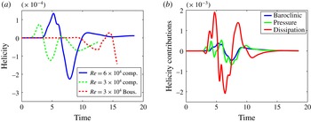
Figure 11. Helicity. (a) Helicity evolution versus time of the three simulations,
 $Sr6\text{-}Re6\times 10^{4}$
,
$Sr6\text{-}Re6\times 10^{4}$
,
 $Sr6\text{-}Re3\times 10^{4}$
and
$Sr6\text{-}Re3\times 10^{4}$
and
 $Sr0\text{-}Re3\times 10^{4}$
. The helicity of the
$Sr0\text{-}Re3\times 10^{4}$
. The helicity of the
 $Sr0\text{-}Re3\times 10^{4}$
simulation has been divided by 10 for the sake of clarity. The helicity strongly decays during the RT regime and in a second step due to acoustic waves. In the FD regime, helicity vanishes slowly. (b) Helicity source terms of (4.9), corresponding to the simulation
$Sr0\text{-}Re3\times 10^{4}$
simulation has been divided by 10 for the sake of clarity. The helicity strongly decays during the RT regime and in a second step due to acoustic waves. In the FD regime, helicity vanishes slowly. (b) Helicity source terms of (4.9), corresponding to the simulation
 $Sr6\text{-}Re6\times 10^{4}$
. Baroclinic source term (blue), pressure source term (green) and dissipation (red). The detailed behaviour of these three contributions depends on the value of
$Sr6\text{-}Re6\times 10^{4}$
. Baroclinic source term (blue), pressure source term (green) and dissipation (red). The detailed behaviour of these three contributions depends on the value of
 $\unicode[STIX]{x1D6FD}$
(not included), but not the global evolution.
$\unicode[STIX]{x1D6FD}$
(not included), but not the global evolution.
4.6 Helicity
The helicity is one of the quantities built from the vorticity and it is defined as
 ${\mathcal{H}}=\int _{{\mathcal{V}}}u_{i}\unicode[STIX]{x1D714}_{i}\,\text{d}V$
. This is a conserved quantity for an inviscid barotropic fluid (Moffatt & Tsinober Reference Moffatt and Tsinober1992) and its evolution equation is written
${\mathcal{H}}=\int _{{\mathcal{V}}}u_{i}\unicode[STIX]{x1D714}_{i}\,\text{d}V$
. This is a conserved quantity for an inviscid barotropic fluid (Moffatt & Tsinober Reference Moffatt and Tsinober1992) and its evolution equation is written
 $$\begin{eqnarray}\displaystyle \frac{\text{d}{\mathcal{H}}}{\text{d}t} & = & \displaystyle \frac{1}{Sr}\displaystyle \int _{{\mathcal{V}}}\frac{1}{\unicode[STIX]{x1D70C}^{2}}\unicode[STIX]{x1D700}_{ijk}u_{i}\unicode[STIX]{x2202}_{j}\unicode[STIX]{x1D70C}\unicode[STIX]{x2202}_{k}p\,\text{d}V-\frac{1}{Sr}\displaystyle \int _{{\mathcal{V}}}\frac{\unicode[STIX]{x1D714}_{i}}{\unicode[STIX]{x1D70C}}\unicode[STIX]{x2202}_{i}p\,\text{d}V\nonumber\\ \displaystyle & & \displaystyle -\,\frac{2}{Re}\displaystyle \int _{{\mathcal{V}}}\unicode[STIX]{x2202}_{j}\left(\frac{\unicode[STIX]{x1D714}_{i}}{\unicode[STIX]{x1D70C}}\right)\unicode[STIX]{x1D70E}_{ij}\,\text{d}V.\end{eqnarray}$$
The first term on the right-hand side is the baroclinic helicity production, the second term comes from pressure forces and the third is the dissipation. Notice that the pressure term vanishes for a fluid of uniform density. The evolution of the helicity is displayed in figure 11(a) for the three simulations. Helicity of the
 $Sr6\text{-}Re6\times 10^{4}$
simulation starts growing at
$Sr6\text{-}Re6\times 10^{4}$
simulation starts growing at
 $t\approx 3.35$
, where the large-scale
$t\approx 3.35$
, where the large-scale
 $A_{LS}$
Atwood number vanishes (
$A_{LS}$
Atwood number vanishes (
 $t\approx 3.55$
). A similar evolution is observed in the two compressible simulations,
$t\approx 3.55$
). A similar evolution is observed in the two compressible simulations,
 $Sr6\text{-}Re6\times 10^{4}$
and
$Sr6\text{-}Re6\times 10^{4}$
and
 $Sr6\text{-}Re3\times 10^{4}$
. They however differ by a time lag of
$Sr6\text{-}Re3\times 10^{4}$
. They however differ by a time lag of
 $\unicode[STIX]{x0394}t\approx 3$
due to different initial conditions (see § 3.3) and the amplitude of the
$\unicode[STIX]{x0394}t\approx 3$
due to different initial conditions (see § 3.3) and the amplitude of the
 $Sr6\text{-}Re6\times 10^{4}$
helicity is larger by a factor
$Sr6\text{-}Re6\times 10^{4}$
helicity is larger by a factor
 ${\approx}1.8$
due to a larger Reynolds number. This growth occurs after the RT regime, defined by the evolution of the large-scale
${\approx}1.8$
due to a larger Reynolds number. This growth occurs after the RT regime, defined by the evolution of the large-scale
 $A_{LS}$
Atwood number. The helicity grows between
$A_{LS}$
Atwood number. The helicity grows between
 $t\approx 5.2$
and
$t\approx 5.2$
and
 $t\approx 7.7$
. This time interval corresponds to the highest values of the vertical Taylor–Reynolds number,
$t\approx 7.7$
. This time interval corresponds to the highest values of the vertical Taylor–Reynolds number,
 $Re_{Tz}$
, (figure 6). It also corresponds to the growth of the mixing layer thickness (figure 5). Beyond that point
$Re_{Tz}$
, (figure 6). It also corresponds to the growth of the mixing layer thickness (figure 5). Beyond that point
 $t\approx 7.7$
, the flow is stabilizing, velocity and vorticity decay and so does the helicity. The helicity of the Boussinesq simulation,
$t\approx 7.7$
, the flow is stabilizing, velocity and vorticity decay and so does the helicity. The helicity of the Boussinesq simulation,
 $Sr0\text{-}Re3\times 10^{4}$
, starts after a long transient and grows rapidly to negative values and reaches, at the end of the simulation, a monotonic behaviour. It is worth noticing that positive (respectively negative) helicity values occur when velocity and vorticity are mainly parallel (respectively anti-parallel). The evolution of the three helicity source terms of equation (4.9), are displayed in figure 11(b) for the
$Sr0\text{-}Re3\times 10^{4}$
, starts after a long transient and grows rapidly to negative values and reaches, at the end of the simulation, a monotonic behaviour. It is worth noticing that positive (respectively negative) helicity values occur when velocity and vorticity are mainly parallel (respectively anti-parallel). The evolution of the three helicity source terms of equation (4.9), are displayed in figure 11(b) for the
 $Sr6\text{-}Re6\times 10^{4}$
simulation. The baroclinic and pressure source terms (first and second terms of the right-hand side, equation (4.9)) are of the same order, while dissipation is dominant. This explains why the first helicity decay regime is close to the RT Boussinesq turbulence. Indeed, since the velocity divergence is small, dissipation terms in the compressible and incompressible flows are close to each other.
$Sr6\text{-}Re6\times 10^{4}$
simulation. The baroclinic and pressure source terms (first and second terms of the right-hand side, equation (4.9)) are of the same order, while dissipation is dominant. This explains why the first helicity decay regime is close to the RT Boussinesq turbulence. Indeed, since the velocity divergence is small, dissipation terms in the compressible and incompressible flows are close to each other.

Figure 12. (a) Comparison of the evolution of the palinstrophy norm in linear–log scales for the three simulations,
 $Sr6\text{-}Re6\times 10^{4}$
,
$Sr6\text{-}Re6\times 10^{4}$
,
 $Sr6\text{-}Re3\times 10^{4}$
and
$Sr6\text{-}Re3\times 10^{4}$
and
 $Sr0\text{-}Re3\times 10^{4}$
. (b) Palinstrophy isosurface at time
$Sr0\text{-}Re3\times 10^{4}$
. (b) Palinstrophy isosurface at time
 $t=4.35$
, coloured by the concentration.
$t=4.35$
, coloured by the concentration.
4.7 Palinstrophy
The palinstrophy density is defined as
 $1/2(\unicode[STIX]{x1D735}\times \unicode[STIX]{x1D74E})^{2}$
, while the palinstrophy is (Lesieur Reference Lesieur1997)
$1/2(\unicode[STIX]{x1D735}\times \unicode[STIX]{x1D74E})^{2}$
, while the palinstrophy is (Lesieur Reference Lesieur1997)
 $$\begin{eqnarray}P(t)=\frac{1}{2}\displaystyle \int _{{\mathcal{V}}}(\unicode[STIX]{x1D735}\times \unicode[STIX]{x1D74E})^{2}\,\text{d}V.\end{eqnarray}$$
Palinstrophy density emphasizes the tightening of vorticity contours. It helps to reveal the structure of a vortical flow (Shipton Reference Shipton2009). Indeed, palinstrophy is built from high-order derivatives, namely the second-order velocity derivative squared, which strongly emphasizes small scales. As such, palinstrophy density is an accurate criteria to detect flow structures. Moreover palinstrophy appears in the enstrophy evolution equation and it is related to the energy spectrum (Lesieur Reference Lesieur1997, § VI-7). The evolution of the palinstrophy is displayed in figure 12(a) in linear–log scales for the three simulations. The palinstrophy of the
 $Sr6\text{-}Re6\times 10^{4}$
simulation reaches its maximum
$Sr6\text{-}Re6\times 10^{4}$
simulation reaches its maximum
 $P_{max}(t_{m})=0.104\times 10^{7}$
at time
$P_{max}(t_{m})=0.104\times 10^{7}$
at time
 $t_{m}\approx 4.10$
, slightly before the vorticity maximum (
$t_{m}\approx 4.10$
, slightly before the vorticity maximum (
 $t\approx 4.35$
). It then decays monotonically to small values, i.e.
$t\approx 4.35$
). It then decays monotonically to small values, i.e.
 $P(t=18.55)=0.968\times 10^{3}$
, at the end of the simulation. The evolution of the palinstrophy of the
$P(t=18.55)=0.968\times 10^{3}$
, at the end of the simulation. The evolution of the palinstrophy of the
 $Sr6\text{-}Re3\times 10^{4}$
simulation is similar with a time shift of
$Sr6\text{-}Re3\times 10^{4}$
simulation is similar with a time shift of
 $\unicode[STIX]{x0394}t=1.62$
and a factor 5 in amplitude. As we have already said, these shifts are due to different initial conditions and different Reynolds numbers, respectively. The Boussinesq-
$\unicode[STIX]{x0394}t=1.62$
and a factor 5 in amplitude. As we have already said, these shifts are due to different initial conditions and different Reynolds numbers, respectively. The Boussinesq-
 $Sr0\text{-}Re3\times 10^{4}$
palinstrophy grows monotonically and an approximate exponential behaviour is observed from time
$Sr0\text{-}Re3\times 10^{4}$
palinstrophy grows monotonically and an approximate exponential behaviour is observed from time
 $t\approx 11$
, in the turbulent regime. Spatial profiles of the palinstrophy density are very similar to those of other variables, see for example the kinetic energy profiles in figure 7. Indeed maximum values are reached approximately at the mixing layer core and decay rapidly toward both layer edges. Figure 12(b) displays the palinstrophy isosurface at time
$t\approx 11$
, in the turbulent regime. Spatial profiles of the palinstrophy density are very similar to those of other variables, see for example the kinetic energy profiles in figure 7. Indeed maximum values are reached approximately at the mixing layer core and decay rapidly toward both layer edges. Figure 12(b) displays the palinstrophy isosurface at time
 $t=4.35$
, coloured by the concentration. It indeed emphasizes small scales.
$t=4.35$
, coloured by the concentration. It indeed emphasizes small scales.

Figure 13. (a) Density fluctuation spectra. The dashed straight line represents the
 $-5/3$
power law. (b) Pressure fluctuation spectra. The dashed straight line represents the
$-5/3$
power law. (b) Pressure fluctuation spectra. The dashed straight line represents the
 $-7/3$
power law. The vertical dashed lines stand for the horizontal and vertical Taylor wavenumbers and the horizontal and vertical Taylor mixing wavenumbers, respectively.
$-7/3$
power law. The vertical dashed lines stand for the horizontal and vertical Taylor wavenumbers and the horizontal and vertical Taylor mixing wavenumbers, respectively.
4.8 One-dimensional spectra
The one-dimensional power spectra of various quantities are reported in this section and compared with classical scalings for the inertial range. Spectra are computed by performing a one-dimensional Fourier transform in an horizontal direction. The result is thus averaged first with respect to the second horizontal direction and a vertical averaging is also performed. Consequently, spectra depend only on the horizontal wavenumber
 $k_{x}$
and on time
$k_{x}$
and on time
 $t$
. Schneider & Gauthier (Reference Schneider and Gauthier2016c
) have shown, for a RT Boussinesq turbulence, that the spectra obtained from the above procedure do not depend on the proportion of the mixing layer on which the average is performed. On the other hand, comparisons between numerical results and classical scalings are often difficult, since the inertial range is often narrow. This is the case here, where the comparison is made difficult by the modest Reynolds number reached, the flow unsteadiness and the compressibility effects, i.e. the variable density and the acoustics, even if the latter is weak. The density fluctuation spectra, at selected times, are represented in figure 13 with the Kolmogorov–Obukhov (KO) law,
$t$
. Schneider & Gauthier (Reference Schneider and Gauthier2016c
) have shown, for a RT Boussinesq turbulence, that the spectra obtained from the above procedure do not depend on the proportion of the mixing layer on which the average is performed. On the other hand, comparisons between numerical results and classical scalings are often difficult, since the inertial range is often narrow. This is the case here, where the comparison is made difficult by the modest Reynolds number reached, the flow unsteadiness and the compressibility effects, i.e. the variable density and the acoustics, even if the latter is weak. The density fluctuation spectra, at selected times, are represented in figure 13 with the Kolmogorov–Obukhov (KO) law,
 $E(k)=k^{-5/3}$
, in the inertial range. The best agreement may be found at short times, at
$E(k)=k^{-5/3}$
, in the inertial range. The best agreement may be found at short times, at
 $t=4.15$
(density fluctuation maximum on the very interior of the mixing layer) and at
$t=4.15$
(density fluctuation maximum on the very interior of the mixing layer) and at
 $t=4.35$
(vorticity maximum). Such agreement is not observed at later times where the Taylor-based Reynolds number is larger. At the maximum of this Reynolds number,
$t=4.35$
(vorticity maximum). Such agreement is not observed at later times where the Taylor-based Reynolds number is larger. At the maximum of this Reynolds number,
 $t=8.30$
, the result is quite similar (not included). Pressure power spectra are given in figure 13(b) at the same three different times. The
$t=8.30$
, the result is quite similar (not included). Pressure power spectra are given in figure 13(b) at the same three different times. The
 $k^{-7/3}$
-scaling obtained from a quasi-normal approximation within an incompressible isotropic turbulence (Batchelor Reference Batchelor1971), (Leslie Reference Leslie1973, § 11.5) have been added. For weakly incompressible turbulence, it has been shown by Bataille, Bertoglio & Marion (Reference Bataille, Bertoglio and Marion1992) that the pressure spectra behave as
$k^{-7/3}$
-scaling obtained from a quasi-normal approximation within an incompressible isotropic turbulence (Batchelor Reference Batchelor1971), (Leslie Reference Leslie1973, § 11.5) have been added. For weakly incompressible turbulence, it has been shown by Bataille, Bertoglio & Marion (Reference Bataille, Bertoglio and Marion1992) that the pressure spectra behave as
 $k^{-5/3}$
in the inertial range and it evolves toward
$k^{-5/3}$
in the inertial range and it evolves toward
 $k^{-11/3}$
at large times. These two scalings have been represented in figure 13(b) in blue and red, respectively. The numerical results are not incompatible with such scalings. A spectral blocking (Boyd Reference Boyd2000, § 11.3) of the pressure power spectra is observed. This is related to insufficient resolution since both turbulent and acoustic signals have to be resolved. The requirements for acoustic wave resolution are more severe than those for turbulent velocity fluctuations. This spectral blocking is thus probably due to the weak resolution of the high frequency acoustic waves. Nevertheless this spectrum spreads over 13 decades. The velocity fluctuation spectra, at selected times, are represented in figure 14 with the KO-scaling
$k^{-11/3}$
at large times. These two scalings have been represented in figure 13(b) in blue and red, respectively. The numerical results are not incompatible with such scalings. A spectral blocking (Boyd Reference Boyd2000, § 11.3) of the pressure power spectra is observed. This is related to insufficient resolution since both turbulent and acoustic signals have to be resolved. The requirements for acoustic wave resolution are more severe than those for turbulent velocity fluctuations. This spectral blocking is thus probably due to the weak resolution of the high frequency acoustic waves. Nevertheless this spectrum spreads over 13 decades. The velocity fluctuation spectra, at selected times, are represented in figure 14 with the KO-scaling
 $k^{-5/3}$
. No agreement is found for the reasons recalled above. Finally, the power spectra of the scalar fluctuations, concentration and temperature, are displayed in figure 15, with the
$k^{-5/3}$
. No agreement is found for the reasons recalled above. Finally, the power spectra of the scalar fluctuations, concentration and temperature, are displayed in figure 15, with the
 $k^{-17/3}$
-scaling (Batchelor, Howells & Townsend Reference Batchelor, Howells and Townsend1959; Ristorcelli Reference Ristorcelli2006). These two sets of concentration and temperature spectra are very similar for the three times displayed, which shows that concentration and temperature behave and evolve closely. The classical
$k^{-17/3}$
-scaling (Batchelor, Howells & Townsend Reference Batchelor, Howells and Townsend1959; Ristorcelli Reference Ristorcelli2006). These two sets of concentration and temperature spectra are very similar for the three times displayed, which shows that concentration and temperature behave and evolve closely. The classical
 $k^{-17/3}$
-scaling is encouraging, although agreement is observed on a very narrow spectral region.
$k^{-17/3}$
-scaling is encouraging, although agreement is observed on a very narrow spectral region.

Figure 14. Velocity fluctuation spectra. (a) Horizontal velocity,
 $\sqrt{\unicode[STIX]{x1D70C}}u_{x}$
, spectra. The dashed straight line represents the
$\sqrt{\unicode[STIX]{x1D70C}}u_{x}$
, spectra. The dashed straight line represents the
 $-$
5/3 power law. The vertical dashed lines stand for the horizontal and vertical Taylor wavenumbers and the horizontal and vertical Taylor mixing wavenumbers, respectively. (b) Vertical velocity,
$-$
5/3 power law. The vertical dashed lines stand for the horizontal and vertical Taylor wavenumbers and the horizontal and vertical Taylor mixing wavenumbers, respectively. (b) Vertical velocity,
 $\sqrt{\unicode[STIX]{x1D70C}}u_{z}$
, spectra.
$\sqrt{\unicode[STIX]{x1D70C}}u_{z}$
, spectra.

Figure 15. Spectra of concentration (a) and temperature (b) fluctuations. The dashed straight line represents the
 $-$
17/3 power law. The vertical dashed lines stand for the horizontal and vertical Taylor wavenumbers and the horizontal and vertical Taylor mixing wavenumbers, respectively. These two sets of spectra are very close to each other.
$-$
17/3 power law. The vertical dashed lines stand for the horizontal and vertical Taylor wavenumbers and the horizontal and vertical Taylor mixing wavenumbers, respectively. These two sets of spectra are very close to each other.

Figure 16. Reynolds stress anisotropy tensor defined by (5.1). (a) Vertical profiles of the diagonal component
 $\unicode[STIX]{x1D609}_{zz}$
, at six different times. (b) Evolution of the
$\unicode[STIX]{x1D609}_{zz}$
, at six different times. (b) Evolution of the
 $\unicode[STIX]{x1D623}_{zz}$
(black),
$\unicode[STIX]{x1D623}_{zz}$
(black),
 $\unicode[STIX]{x1D623}_{yy}$
(green) and
$\unicode[STIX]{x1D623}_{yy}$
(green) and
 $\unicode[STIX]{x1D623}_{yz}$
(blue) components, as defined in (5.1).
$\unicode[STIX]{x1D623}_{yz}$
(blue) components, as defined in (5.1).
5 Anisotropy
Since the flow and mixing anisotropies are a current concern in RT-induced turbulent mixing layers, this point is considered in this section. We use the Reynolds stress anisotropy tensor for the velocity, where no distinction between the various scales is made. We also use a spectral anisotropy indicator for the velocity and the scalars, to have access to the anisotropy of a given scale. The horizontal,
 $\unicode[STIX]{x1D609}_{ij}(z,t)$
and volume average,
$\unicode[STIX]{x1D609}_{ij}(z,t)$
and volume average,
 $\unicode[STIX]{x1D623}_{ij}(t)$
, of the Reynolds stress anisotropy tensor are defined as
$\unicode[STIX]{x1D623}_{ij}(t)$
, of the Reynolds stress anisotropy tensor are defined as
 $$\begin{eqnarray}\unicode[STIX]{x1D609}_{ij}(z,t)=\frac{\overline{\unicode[STIX]{x1D70C}u_{i}^{\prime \prime }u_{j}^{\prime \prime }}}{2\overline{\unicode[STIX]{x1D70C}}\widetilde{k}}-\frac{1}{3}\unicode[STIX]{x1D6FF}_{ij}\quad \text{and}\quad \unicode[STIX]{x1D623}_{ij}(t)=\frac{\langle \overline{\unicode[STIX]{x1D70C}u_{i}^{\prime \prime }u_{j}^{\prime \prime }}\rangle }{2\langle \overline{\unicode[STIX]{x1D70C}}\widetilde{k}\rangle }-\frac{1}{3}\unicode[STIX]{x1D6FF}_{ij}.\end{eqnarray}$$
Vertical profiles of the
 $\unicode[STIX]{x1D609}_{zz}$
-component are displayed in figure 16(a) at six different times. Notice that expressions (5.1) are defined for all values of the
$\unicode[STIX]{x1D609}_{zz}$
-component are displayed in figure 16(a) at six different times. Notice that expressions (5.1) are defined for all values of the
 $z$
-coordinate, although outside of the turbulent mixing layer the three contributions of the turbulent kinetic energy are very small. At
$z$
-coordinate, although outside of the turbulent mixing layer the three contributions of the turbulent kinetic energy are very small. At
 $t=3.25$
, turbulence anisotropy reaches 0.55, which means that
$t=3.25$
, turbulence anisotropy reaches 0.55, which means that
 $88\,\%$
of the turbulent kinetic energy is in the third direction, while at
$88\,\%$
of the turbulent kinetic energy is in the third direction, while at
 $t=7.45$
,
$t=7.45$
,
 $64\,\%$
of the turbulent kinetic energy is in the third direction. The time evolution of the three components of the mean value
$64\,\%$
of the turbulent kinetic energy is in the third direction. The time evolution of the three components of the mean value
 $\unicode[STIX]{x1D623}_{ij}$
are represented in figure 16(b). It also shows a strong anisotropy during the RT regime, where the kinetic energy corresponding to the vertical direction is about
$\unicode[STIX]{x1D623}_{ij}$
are represented in figure 16(b). It also shows a strong anisotropy during the RT regime, where the kinetic energy corresponding to the vertical direction is about
 $90\,\%$
of the total turbulent kinetic energy. After this maximum, the anisotropy abruptly decreases to
$90\,\%$
of the total turbulent kinetic energy. After this maximum, the anisotropy abruptly decreases to
 $\unicode[STIX]{x1D623}_{zz}\approx 0.40$
between
$\unicode[STIX]{x1D623}_{zz}\approx 0.40$
between
 $t\approx 3$
and 4. Afterwards, the isotropy is slowly re-established meanwhile turbulence is decaying. The horizontal diagonal Reynolds stress anisotropy tensor components,
$t\approx 3$
and 4. Afterwards, the isotropy is slowly re-established meanwhile turbulence is decaying. The horizontal diagonal Reynolds stress anisotropy tensor components,
 $\unicode[STIX]{x1D623}_{xx}$
and
$\unicode[STIX]{x1D623}_{xx}$
and
 $\unicode[STIX]{x1D623}_{yy}$
, are very closed to each other (not included), all along the process. The off-diagonal term,
$\unicode[STIX]{x1D623}_{yy}$
, are very closed to each other (not included), all along the process. The off-diagonal term,
 $\unicode[STIX]{x1D623}_{yz}$
(or
$\unicode[STIX]{x1D623}_{yz}$
(or
 $\unicode[STIX]{x1D623}_{xz}$
), is negligible at all times, which shows that turbulence production is essentially, or totally, of baroclinic type, no shear production occurs here. On the other hand, it has already been shown that intermediate scales are isotropic while small scales are not, at low and large Atwood numbers, within the Sandoval model (Livescu & Ristorcelli Reference Livescu and Ristorcelli2008; Chung & Pullin Reference Chung and Pullin2010; Livescu et al.
Reference Livescu, Ristorcelli, Petersen and Gore2010). Similar conclusions have also been drawn from a RT Boussinesq large-scale simulation (Schneider & Gauthier Reference Schneider and Gauthier2016a
). This anisotropy is stronger in the middle of the mixing layer where turbulence is stronger. In addition, in this compressible case, acoustic waves may also contribute to this anisotropy.
$\unicode[STIX]{x1D623}_{xz}$
), is negligible at all times, which shows that turbulence production is essentially, or totally, of baroclinic type, no shear production occurs here. On the other hand, it has already been shown that intermediate scales are isotropic while small scales are not, at low and large Atwood numbers, within the Sandoval model (Livescu & Ristorcelli Reference Livescu and Ristorcelli2008; Chung & Pullin Reference Chung and Pullin2010; Livescu et al.
Reference Livescu, Ristorcelli, Petersen and Gore2010). Similar conclusions have also been drawn from a RT Boussinesq large-scale simulation (Schneider & Gauthier Reference Schneider and Gauthier2016a
). This anisotropy is stronger in the middle of the mixing layer where turbulence is stronger. In addition, in this compressible case, acoustic waves may also contribute to this anisotropy.

Figure 17. Velocity spectral anisotropy, as defined by (5.2), at four different times,
 $t=4.35$
(first vorticity maximum),
$t=4.35$
(first vorticity maximum),
 $t=6.85$
(second vorticity maximum),
$t=6.85$
(second vorticity maximum),
 $t=7.45$
(kinetic energy maximum) and
$t=7.45$
(kinetic energy maximum) and
 $t=11$
(within the FD regime).
$t=11$
(within the FD regime).
Spectral anisotropy has been investigated by several authors (Livescu & Ristorcelli Reference Livescu and Ristorcelli2008; Chung & Pullin Reference Chung and Pullin2010; Livescu et al. Reference Livescu, Ristorcelli, Petersen and Gore2010; Cabot & Zhou Reference Cabot and Zhou2013). The following indicator for the velocity anisotropy (Chung & Pullin Reference Chung and Pullin2010; Schneider & Gauthier Reference Schneider and Gauthier2016c ) is used
 $$\begin{eqnarray}S_{u}(k_{x},t)=\frac{\langle \widehat{u}_{3}^{2}(k_{x},k_{y}=0,z,t)\rangle }{\displaystyle \mathop{\sum }_{i=1}^{3}\langle \widehat{u}_{i}^{2}(k_{x},k_{y}=0,z,t)\rangle }-\frac{1}{3},\end{eqnarray}$$
where
 $\widehat{u}$
denotes the Fourier transform of the vector variable
$\widehat{u}$
denotes the Fourier transform of the vector variable
 $u$
. Results for the velocity anisotropy,
$u$
. Results for the velocity anisotropy,
 $S_{u}(k_{x},t)$
, are shown in figure 17, at four different times,
$S_{u}(k_{x},t)$
, are shown in figure 17, at four different times,
 $t=4.35$
(first vorticity maximum),
$t=4.35$
(first vorticity maximum),
 $t=6.85$
(second vorticity maximum),
$t=6.85$
(second vorticity maximum),
 $t=7.45$
(kinetic energy maximum) and
$t=7.45$
(kinetic energy maximum) and
 $t=11$
(within the FD regime). At any time, the intermediate scales are isotropic, as opposed to the RT Boussinesq turbulence (Schneider & Gauthier Reference Schneider and Gauthier2016c
). However, from time
$t=11$
(within the FD regime). At any time, the intermediate scales are isotropic, as opposed to the RT Boussinesq turbulence (Schneider & Gauthier Reference Schneider and Gauthier2016c
). However, from time
 $t=7.45$
, intermediate scales are more isotropic than the small scales. Within the FD regime, all scales are slightly anisotropic. The scalar anisotropy is evaluated with the following indicator
$t=7.45$
, intermediate scales are more isotropic than the small scales. Within the FD regime, all scales are slightly anisotropic. The scalar anisotropy is evaluated with the following indicator
 $$\begin{eqnarray}S_{\unicode[STIX]{x1D735}c}(k_{x},t)=\frac{\langle \widehat{\unicode[STIX]{x1D6FB}_{3}c}^{2}(k_{x},k_{y}=0,z,t)\rangle }{\displaystyle \mathop{\sum }_{i=1}^{3}\langle \widehat{\unicode[STIX]{x1D6FB}_{i}c}^{2}(k_{x},k_{y}=0,z,t)\rangle }-\frac{1}{3}.\end{eqnarray}$$
similar to equation (5.2). The anisotropy variations with respect to the horizontal wavenumber
 $k_{x}$
are shown in figures 18 and 19 for the concentration and temperature. Isotropy clearly occurs at intermediate scales only, for the four times displayed and for the two scalars, concentration and temperature. We notice a very strong resemblance between the concentration and temperature spectra at a given time. Very similar results have been obtained for the Boussinesq simulation,
$k_{x}$
are shown in figures 18 and 19 for the concentration and temperature. Isotropy clearly occurs at intermediate scales only, for the four times displayed and for the two scalars, concentration and temperature. We notice a very strong resemblance between the concentration and temperature spectra at a given time. Very similar results have been obtained for the Boussinesq simulation,
 $Sr0\text{-}Re3\times 10^{4}$
, and the compressible simulation,
$Sr0\text{-}Re3\times 10^{4}$
, and the compressible simulation,
 $Sr6\text{-}Re3\times 10^{4}$
.
$Sr6\text{-}Re3\times 10^{4}$
.

Figure 18. Concentration-gradient spectral anisotropy, as defined by (5.3), at four different times,
 $t=4.35$
,
$t=4.35$
,
 $6.85$
,
$6.85$
,
 $7.45$
and
$7.45$
and
 $11$
.
$11$
.

Figure 19. Temperature-gradient spectral anisotropy, as defined by (5.3), at four different times,
 $t=4.35$
,
$t=4.35$
,
 $6.85$
,
$6.85$
,
 $7.45$
and
$7.45$
and
 $11$
.
$11$
.
6 Averaged turbulent equations
In this section, the numerical data are further analysed by using the Favre-averaged equations. Such an analysis is also relevant for second-order modelling (Grégoire, Souffland & Gauthier Reference Grégoire, Souffland and Gauthier2005; Livescu et al. Reference Livescu, Ristorcelli, Petersen and Gore2010). The equation for the turbulent kinetic energy is first recalled. The right-hand side of this equation contains the three families of terms, i.e. production, diffusion and dissipation. From equations (2.5) and definition (2.10), one obtains the exact averaged equation for the turbulent kinetic energy (Chassaing et al. Reference Chassaing, Antonia, Anselmet, Joly and Sarkar2002, § 5.7)
 $$\begin{eqnarray}\displaystyle \unicode[STIX]{x2202}_{t}\overline{\unicode[STIX]{x1D70C}}\widetilde{k}+\unicode[STIX]{x2202}_{j}\overline{\unicode[STIX]{x1D70C}}\widetilde{u}_{j}\widetilde{k} & = & \displaystyle -\overline{\unicode[STIX]{x1D70C}u_{i}^{\prime \prime }u_{j}^{\prime \prime }}\unicode[STIX]{x2202}_{j}\widetilde{u}_{i}-\frac{1}{Sr}\overline{u_{i}^{\prime \prime }}\unicode[STIX]{x2202}_{i}\overline{p}\nonumber\\ \displaystyle & & \displaystyle -\,\unicode[STIX]{x2202}_{i}\left(\overline{\unicode[STIX]{x1D70C}u_{i}^{\prime \prime }k^{\prime \prime }}+\frac{1}{Sr}\overline{u_{i}^{\prime \prime }p^{\prime }}+\frac{1}{Re}\overline{u_{j}^{\prime \prime }\unicode[STIX]{x1D70E}_{ij}}\right)+\frac{1}{Sr}\overline{p^{\prime }\unicode[STIX]{x2202}_{i}u_{i}^{\prime \prime }}-\overline{\unicode[STIX]{x1D70C}}\widetilde{\unicode[STIX]{x1D700}},\end{eqnarray}$$
where the expression of the dissipation rate is
 $$\begin{eqnarray}\overline{\unicode[STIX]{x1D70C}}\widetilde{\unicode[STIX]{x1D700}}=\frac{1}{Re}\overline{\unicode[STIX]{x2202}_{i}u_{j}^{\prime \prime }\unicode[STIX]{x1D70E}_{ij}}.\end{eqnarray}$$
The first two terms of the right-hand side of equation (6.1) are producing turbulence, one from the velocity shear, the second from the baroclinic term. The third contribution is the diffusion term, then the pressure velocity–divergence correlation, which is mainly a dissipation term, and the viscous dissipation. The evolution of the turbulent kinetic energy
 $\langle k\rangle _{\unicode[STIX]{x1D6FD}}$
of the three simulations,
$\langle k\rangle _{\unicode[STIX]{x1D6FD}}$
of the three simulations,
 $Sr6\text{-}Re6\times 10^{4}$
,
$Sr6\text{-}Re6\times 10^{4}$
,
 $Sr6\text{-}Re3\times 10^{4}$
and
$Sr6\text{-}Re3\times 10^{4}$
and
 $Sr0\text{-}Re3\times 10^{4}$
, are given in figure 20. The kinetic energy of the
$Sr0\text{-}Re3\times 10^{4}$
, are given in figure 20. The kinetic energy of the
 $Sr6\text{-}Re6\times 10^{4}$
-simulation grows during the RT regime and reaches a first maximum at
$Sr6\text{-}Re6\times 10^{4}$
-simulation grows during the RT regime and reaches a first maximum at
 $t\approx 3.9$
. A second peak is reached at
$t\approx 3.9$
. A second peak is reached at
 $t\approx 6.55$
, essentially due to acoustic waves. Similar evolution is obtained from the compressible run,
$t\approx 6.55$
, essentially due to acoustic waves. Similar evolution is obtained from the compressible run,
 $Sr6\text{-}Re3\times 10^{4}$
. The same amplitude is observed in these two simulations with a time shift of
$Sr6\text{-}Re3\times 10^{4}$
. The same amplitude is observed in these two simulations with a time shift of
 $\unicode[STIX]{x0394}t\approx 1.40$
. These evolutions are different to the one obtained from the Boussinesq approximation where the turbulent kinetic energy grows as
$\unicode[STIX]{x0394}t\approx 1.40$
. These evolutions are different to the one obtained from the Boussinesq approximation where the turbulent kinetic energy grows as
 $t^{2}$
in the turbulent regime. Dissipation rates of the two compressible runs have the same behaviour, i.e. a strong increase in the RT regime followed by two maxima and the FD regime. They also differ from a time shift of
$t^{2}$
in the turbulent regime. Dissipation rates of the two compressible runs have the same behaviour, i.e. a strong increase in the RT regime followed by two maxima and the FD regime. They also differ from a time shift of
 $\unicode[STIX]{x0394}t\approx 1.40$
with a factor 1.08 in amplitude. The dissipation rate behaviour obtained from the Boussinesq approximation grows as
$\unicode[STIX]{x0394}t\approx 1.40$
with a factor 1.08 in amplitude. The dissipation rate behaviour obtained from the Boussinesq approximation grows as
 $t$
at a much larger level. The turnover time scale is estimated as the ratio
$t$
at a much larger level. The turnover time scale is estimated as the ratio
 $\langle \widetilde{k}/\widetilde{\unicode[STIX]{x1D700}}\rangle _{\unicode[STIX]{x1D6FD}}$
and its initial value is often used to measure a flow duration. If we assume that the flow is turbulent when the Taylor–Reynolds number reaches
$\langle \widetilde{k}/\widetilde{\unicode[STIX]{x1D700}}\rangle _{\unicode[STIX]{x1D6FD}}$
and its initial value is often used to measure a flow duration. If we assume that the flow is turbulent when the Taylor–Reynolds number reaches
 $Re_{Tz}\approx 30$
(
$Re_{Tz}\approx 30$
(
 $t=2.55$
), the initial turnover time scale is
$t=2.55$
), the initial turnover time scale is
 $\unicode[STIX]{x1D70F}_{turn-over}=0.43$
. The RT regime thus undergoes several turnover time scales. At later times, the turnover time scale grows continuously and is equal to
$\unicode[STIX]{x1D70F}_{turn-over}=0.43$
. The RT regime thus undergoes several turnover time scales. At later times, the turnover time scale grows continuously and is equal to
 $\unicode[STIX]{x1D70F}_{turnover}=2.69$
at time
$\unicode[STIX]{x1D70F}_{turnover}=2.69$
at time
 $t=3.25$
,
$t=3.25$
,
 $\unicode[STIX]{x1D70F}_{turnover}=4.45$
(
$\unicode[STIX]{x1D70F}_{turnover}=4.45$
(
 $t=4.15$
) and
$t=4.15$
) and
 $\unicode[STIX]{x1D70F}_{turnover}=13.0$
(
$\unicode[STIX]{x1D70F}_{turnover}=13.0$
(
 $t=7.45$
). It is still growing during the FD regime, up to
$t=7.45$
). It is still growing during the FD regime, up to
 $t\approx 15$
, where it slowly decays. This remark about the turnover time scales also applies to the
$t\approx 15$
, where it slowly decays. This remark about the turnover time scales also applies to the
 $Sr6\text{-}Re3\times 10^{4}$
simulation.
$Sr6\text{-}Re3\times 10^{4}$
simulation.

Figure 20. (a) Turbulent kinetic energy
 $\overline{\unicode[STIX]{x1D70C}}\widetilde{k}=\overline{\unicode[STIX]{x1D70C}u_{i}^{\prime \prime }u_{i}^{\prime \prime }}/2$
. Comparison between results obtained from simulations
$\overline{\unicode[STIX]{x1D70C}}\widetilde{k}=\overline{\unicode[STIX]{x1D70C}u_{i}^{\prime \prime }u_{i}^{\prime \prime }}/2$
. Comparison between results obtained from simulations
 $Sr6\text{-}Re6\times 10^{4}$
(blue),
$Sr6\text{-}Re6\times 10^{4}$
(blue),
 $Sr6\text{-}Re3\times 10^{4}$
(green) and
$Sr6\text{-}Re3\times 10^{4}$
(green) and
 $Sr0\text{-}Re3\times 10^{4}$
(red). (b) Dissipation rate. Comparison between results obtained from simulations
$Sr0\text{-}Re3\times 10^{4}$
(red). (b) Dissipation rate. Comparison between results obtained from simulations
 $Sr6\text{-}Re6\times 10^{4}$
(blue),
$Sr6\text{-}Re6\times 10^{4}$
(blue),
 $Sr6\text{-}Re3\times 10^{4}$
(green) and
$Sr6\text{-}Re3\times 10^{4}$
(green) and
 $Sr0\text{-}Re3\times 10^{4}$
(red).
$Sr0\text{-}Re3\times 10^{4}$
(red).

Figure 21. Mean profiles related to (6.1). (a) Turbulent kinetic energy
 $\overline{\unicode[STIX]{x1D70C}}\widetilde{k}$
, dissipation rate
$\overline{\unicode[STIX]{x1D70C}}\widetilde{k}$
, dissipation rate
 $\overline{\unicode[STIX]{x1D70C}}\widetilde{\unicode[STIX]{x1D700}}$
, pressure source term
$\overline{\unicode[STIX]{x1D70C}}\widetilde{\unicode[STIX]{x1D700}}$
, pressure source term
 $-1/Sr\overline{u_{z}^{\prime }}\unicode[STIX]{x2202}_{z}\overline{p}$
and pressure–velocity divergence correlation
$-1/Sr\overline{u_{z}^{\prime }}\unicode[STIX]{x2202}_{z}\overline{p}$
and pressure–velocity divergence correlation
 $1/Sr\overline{p^{\prime }\unicode[STIX]{x2202}_{i}u_{i}^{\prime }}$
. The mean effective Atwood number
$1/Sr\overline{p^{\prime }\unicode[STIX]{x2202}_{i}u_{i}^{\prime }}$
. The mean effective Atwood number
 $3\times 10^{-3}A_{t}(t)/A_{t}(0)$
versus time is represented by the black dashed curve. (b) Disequilibrium as defined by (6.3) for two values of
$3\times 10^{-3}A_{t}(t)/A_{t}(0)$
versus time is represented by the black dashed curve. (b) Disequilibrium as defined by (6.3) for two values of
 $\unicode[STIX]{x1D6FD}=0.8$
; (blue) and
$\unicode[STIX]{x1D6FD}=0.8$
; (blue) and
 $\unicode[STIX]{x1D6FD}=0.2$
(green). The black dashed line is located at the ordinate 1, the equilibrium value.
$\unicode[STIX]{x1D6FD}=0.2$
(green). The black dashed line is located at the ordinate 1, the equilibrium value.
Mean value evolutions of the source terms of equation (6.1), i.e. turbulent kinetic energy, dissipation rate and production term
 $\overline{u_{z}^{\prime }}\unicode[STIX]{x2202}_{z}\overline{p}$
are given in figure 21(a). The
$\overline{u_{z}^{\prime }}\unicode[STIX]{x2202}_{z}\overline{p}$
are given in figure 21(a). The
 $A_{LS}$
Atwood number computed from the
$A_{LS}$
Atwood number computed from the
 $(x,y)$
-averaged density profile is also plotted. The turbulent kinetic energy exhibits two maxima, the first one is associated with the RT instability, the second with acoustic production. During the RT regime, kinetic energy follows closely the production term,
$(x,y)$
-averaged density profile is also plotted. The turbulent kinetic energy exhibits two maxima, the first one is associated with the RT instability, the second with acoustic production. During the RT regime, kinetic energy follows closely the production term,
 $\overline{u_{z}^{\prime }}\unicode[STIX]{x2202}_{z}\overline{p}$
, while dissipation lags behind. However, from the end of the RT regime, where the large-scale
$\overline{u_{z}^{\prime }}\unicode[STIX]{x2202}_{z}\overline{p}$
, while dissipation lags behind. However, from the end of the RT regime, where the large-scale
 $A_{LS}$
Atwood number vanishes, this production term and the dissipation decay while the kinetic energy is still fed by acoustic waves. Turbulent kinetic energy only decays after its second maximum. Turbulence production from velocity shear is negligible, its maximum is
$A_{LS}$
Atwood number vanishes, this production term and the dissipation decay while the kinetic energy is still fed by acoustic waves. Turbulent kinetic energy only decays after its second maximum. Turbulence production from velocity shear is negligible, its maximum is
 $10^{-4}$
, while baroclinic production maximum is of the order of
$10^{-4}$
, while baroclinic production maximum is of the order of
 $3\times 10^{-3}$
. The pressure velocity–divergence correlation, which would act as a dissipation term during the RT regime, is also negligible. In the FD regime, it produces turbulence at a very small rate, the maximum being
$3\times 10^{-3}$
. The pressure velocity–divergence correlation, which would act as a dissipation term during the RT regime, is also negligible. In the FD regime, it produces turbulence at a very small rate, the maximum being
 $2\times 10^{-4}$
obtained at
$2\times 10^{-4}$
obtained at
 $t\approx 8$
. Classically, the turbulent kinetic energy decay may be fitted with a power law of the form
$t\approx 8$
. Classically, the turbulent kinetic energy decay may be fitted with a power law of the form
 $t^{-n}$
(Kitamura et al.
Reference Kitamura, Nagata, Sakai, Sasoh, Terashima, Saito and Harasaki2014). However, it was not possible to obtain a fit on a reasonable time interval, probably due the perturbation brought by the acoustic waves.
$t^{-n}$
(Kitamura et al.
Reference Kitamura, Nagata, Sakai, Sasoh, Terashima, Saito and Harasaki2014). However, it was not possible to obtain a fit on a reasonable time interval, probably due the perturbation brought by the acoustic waves.
The mixing layer disequilibrium is defined as the ratio of the production to the dissipation (Chung & Pullin Reference Chung and Pullin2010)
 $$\begin{eqnarray}{\mathcal{D}}_{equil.}=\frac{\overline{u_{i}^{\prime \prime }}\unicode[STIX]{x2202}_{i}\overline{p}/Sr}{\overline{\unicode[STIX]{x1D70C}}\widetilde{\unicode[STIX]{x1D700}}}.\end{eqnarray}$$
A turbulent mixing layer is said to be at the equilibrium when the turbulence is produced and dissipated at the same rate, i.e. when
 ${\mathcal{D}}_{equil.}=1$
. This quantity is plotted in figure 21(b) for two values of the coefficient
${\mathcal{D}}_{equil.}=1$
. This quantity is plotted in figure 21(b) for two values of the coefficient
 $\unicode[STIX]{x1D6FD}=0.8$
and 0.2. It turns out that a RT compressible mixing layer is never in equilibrium. Instead strong departures from equilibrium are observed during the RT regime. At the end of this regime the smallest value is
$\unicode[STIX]{x1D6FD}=0.8$
and 0.2. It turns out that a RT compressible mixing layer is never in equilibrium. Instead strong departures from equilibrium are observed during the RT regime. At the end of this regime the smallest value is
 ${\mathcal{D}}_{equil.}=1.22$
at
${\mathcal{D}}_{equil.}=1.22$
at
 $t\approx 4.35$
, which is also the vorticity maximum. At large times, in the FD regime, the source term changes sign and so does the equilibrium parameter.
$t\approx 4.35$
, which is also the vorticity maximum. At large times, in the FD regime, the source term changes sign and so does the equilibrium parameter.

Figure 22. Vertical mean profiles of the r.m.s.-density source terms (equation (6.4)). (a) Density-gradient source term
 $-2\overline{\unicode[STIX]{x1D70C}^{\prime }u_{z}^{\prime }}\unicode[STIX]{x2202}_{z}\bar{\unicode[STIX]{x1D70C}}$
. (b) Velocity-gradient source term
$-2\overline{\unicode[STIX]{x1D70C}^{\prime }u_{z}^{\prime }}\unicode[STIX]{x2202}_{z}\bar{\unicode[STIX]{x1D70C}}$
. (b) Velocity-gradient source term
 $-2\overline{\unicode[STIX]{x1D70C}^{\prime 2}}\unicode[STIX]{x2202}_{z}\tilde{u} _{z}$
.
$-2\overline{\unicode[STIX]{x1D70C}^{\prime 2}}\unicode[STIX]{x2202}_{z}\tilde{u} _{z}$
.
The turbulent kinetic energy equation (6.1) uses the mass flux
 $\overline{\unicode[STIX]{x1D70C}^{\prime }u_{z}^{\prime \prime }}=-\overline{\unicode[STIX]{x1D70C}}\overline{u_{z}^{\prime \prime }}$
in the baroclinic production. It is thus of interest to derive the evolution equation of this quantity and to analyse the production terms. It turns out that this equation contains the r.m.s. density. We thus also derive the evolution equation for this quantity. The equation for the r.m.s. density is
$\overline{\unicode[STIX]{x1D70C}^{\prime }u_{z}^{\prime \prime }}=-\overline{\unicode[STIX]{x1D70C}}\overline{u_{z}^{\prime \prime }}$
in the baroclinic production. It is thus of interest to derive the evolution equation of this quantity and to analyse the production terms. It turns out that this equation contains the r.m.s. density. We thus also derive the evolution equation for this quantity. The equation for the r.m.s. density is
 $$\begin{eqnarray}(\unicode[STIX]{x2202}_{t}+\widetilde{u}_{i}\unicode[STIX]{x2202}_{i})\overline{\unicode[STIX]{x1D70C}^{\prime 2}}=-2\overline{\unicode[STIX]{x1D70C}^{\prime }u_{i}^{\prime \prime }}\unicode[STIX]{x2202}_{i}\overline{\unicode[STIX]{x1D70C}}-2\overline{\unicode[STIX]{x1D70C}^{\prime 2}}\unicode[STIX]{x2202}_{i}\widetilde{u}_{i}+\text{Diffusion}+\text{Dissipation}.\end{eqnarray}$$
The two source terms of the right-hand side are displayed in figure 22 at six selected times. The term proportional to the density gradient follows the RT regime and vanishes at time
 $t\approx 5$
. At time
$t\approx 5$
. At time
 $t=3.25$
, its contribution is small and for larger times, this term becomes a sink for the r.m.s. density. This density-gradient source term is one order of magnitude larger than the velocity-gradient source term. It is a source in the light fluid but a sink in the heavy fluid part. The equation for the mass flux is written (Chassaing et al.
Reference Chassaing, Antonia, Anselmet, Joly and Sarkar2002, § 5.5)
$t=3.25$
, its contribution is small and for larger times, this term becomes a sink for the r.m.s. density. This density-gradient source term is one order of magnitude larger than the velocity-gradient source term. It is a source in the light fluid but a sink in the heavy fluid part. The equation for the mass flux is written (Chassaing et al.
Reference Chassaing, Antonia, Anselmet, Joly and Sarkar2002, § 5.5)
 $$\begin{eqnarray}\overline{\unicode[STIX]{x1D70C}}(\unicode[STIX]{x2202}+\widetilde{u}_{i}\unicode[STIX]{x2202}_{i})\overline{u_{i}^{\prime \prime }}=+\widetilde{u_{i}^{\prime \prime }u_{j}^{\prime \prime }}\unicode[STIX]{x2202}_{j}\overline{\unicode[STIX]{x1D70C}}-\overline{\unicode[STIX]{x1D70C}}\overline{u_{j}^{\prime \prime }}\unicode[STIX]{x2202}_{j}\widetilde{u}_{i}-\frac{\overline{\unicode[STIX]{x1D70C}^{\prime 2}}}{\overline{\unicode[STIX]{x1D70C}}^{2}}\unicode[STIX]{x2202}_{i}\overline{p}+\text{Diffusion}+\text{Dissipation}.\end{eqnarray}$$
Equations (6.4) and (6.5) for the density fluctuations and the mass flux are coupled through their source terms. Density fluctuations and mass flux are mainly created by the density gradient and the pressure gradient, respectively. In a second step, the mass flux and the pressure gradient produce turbulent kinetic energy. The evolution of the three source term mean values of equation (6.5) are represented in figure 23. The term proportional to the pressure gradient is dominant and always positive. Its maximum is reached at
 $t\approx 3.25$
. Production due to the velocity gradient is always negligible. Production due to the density gradient is small, positive in the RT regime and negative in the FD regime. Its maximum is reached very early at
$t\approx 3.25$
. Production due to the velocity gradient is always negligible. Production due to the density gradient is small, positive in the RT regime and negative in the FD regime. Its maximum is reached very early at
 $t\approx 2.80$
.
$t\approx 2.80$
.

Figure 23. Mass flux source terms of equation (6.5). (b) Mean values of the three production terms proportional to the density, vertical velocity and pressure gradients, respectively. The pressure-gradient term is dominant and reaches its maximum at
 $t=3.25$
. (b) Vertical profiles of the mass flux source term proportional to the pressure at six different times.
$t=3.25$
. (b) Vertical profiles of the mass flux source term proportional to the pressure at six different times.
The energy equation is also written as an equation for the Favre-averaged temperature,
 $\widetilde{T}$
. It is written
$\widetilde{T}$
. It is written
 $$\begin{eqnarray}\displaystyle \displaystyle \unicode[STIX]{x2202}_{t}\overline{\unicode[STIX]{x1D70C}}\widetilde{T}+\unicode[STIX]{x2202}_{i}\overline{\unicode[STIX]{x1D70C}}\widetilde{u}_{i}\widetilde{T} & = & \displaystyle -(\unicode[STIX]{x1D6FE}_{r}-1)\overline{\frac{p\unicode[STIX]{x2202}_{i}u_{i}}{C_{v;m}}}+\frac{Sr}{Re}\overline{\frac{\unicode[STIX]{x1D70E}_{ij}\unicode[STIX]{x1D634}_{ij}}{C_{v;m}}}\nonumber\\ \displaystyle & & \displaystyle -\,\frac{d_{c}C_{v;m}}{ReSc}\overline{\frac{T\unicode[STIX]{x2202}_{jj}c}{C_{v;m}}}+\frac{\unicode[STIX]{x1D6E5}_{H,L}^{\star }}{RePr}\overline{\frac{1}{C_{v;m}}\unicode[STIX]{x2202}_{i}[T\unicode[STIX]{x2202}_{i}c]}\nonumber\\ \displaystyle & & \displaystyle +\,\unicode[STIX]{x1D6FE}_{r}RePr\overline{\frac{1}{C_{v;m}}\unicode[STIX]{x2202}_{jj}T}-\unicode[STIX]{x2202}_{i}\overline{\unicode[STIX]{x1D70C}u_{i}^{\prime \prime }T^{\prime \prime }}.\end{eqnarray}$$
The six terms of the right-hand side have been evaluated and the maximum values observed in the interval
 $3.25\leqslant t\leqslant 18.55$
are the following. The
$3.25\leqslant t\leqslant 18.55$
are the following. The
 $p\unicode[STIX]{x2202}_{j}u_{j}$
term is approximately
$p\unicode[STIX]{x2202}_{j}u_{j}$
term is approximately
 $0.10\times 10^{-1}$
. The dissipation function is smaller, i.e.
$0.10\times 10^{-1}$
. The dissipation function is smaller, i.e.
 $0.07\times 10^{-1}$
, the term due to variations of the specific heat is
$0.07\times 10^{-1}$
, the term due to variations of the specific heat is
 $0.20\times 10^{-1}$
, the enthalpic part of the heat flux contribution is
$0.20\times 10^{-1}$
, the enthalpic part of the heat flux contribution is
 $1.50\times 10^{-1}$
, the diffusive contribution is
$1.50\times 10^{-1}$
, the diffusive contribution is
 $0.10\times 10^{-1}$
and the turbulent energy flux,
$0.10\times 10^{-1}$
and the turbulent energy flux,
 $\unicode[STIX]{x2202}_{z}\overline{\unicode[STIX]{x1D70C}u_{z}^{\prime \prime }T^{\prime \prime }}$
is
$\unicode[STIX]{x2202}_{z}\overline{\unicode[STIX]{x1D70C}u_{z}^{\prime \prime }T^{\prime \prime }}$
is
 $0.50\times 10^{-1}$
. The enthalpic part of the heat flux contribution and the turbulent energy flux are therefore the two main contributions. The enthalpic contribution has very large values at the initial times and very quickly decays, while the turbulent thermal flux is zero at the initial time and grows with temperature and velocity fluctuations. To be more precise, at times
$0.50\times 10^{-1}$
. The enthalpic part of the heat flux contribution and the turbulent energy flux are therefore the two main contributions. The enthalpic contribution has very large values at the initial times and very quickly decays, while the turbulent thermal flux is zero at the initial time and grows with temperature and velocity fluctuations. To be more precise, at times
 $t=3.25$
, 4.15 and 8.40, these two contributions have the same magnitude,
$t=3.25$
, 4.15 and 8.40, these two contributions have the same magnitude,
 $(0.015,0.040)$
,
$(0.015,0.040)$
,
 $(0.080,0.055)$
and
$(0.080,0.055)$
and
 $(0.035,0.035)$
, respectively. These relative values can be explained by the modest Reynolds number reached in this simulation. On the other hand, at short times the full right-hand side is negative in the light fluid side and positive in the heavy fluid. At larger times, this is the opposite, the right-hand side is positive in the light fluid and negative in the heavy fluid. Finally the difference between Favre and Reynolds averaging has been evaluated on the temperature. The difference
$(0.035,0.035)$
, respectively. These relative values can be explained by the modest Reynolds number reached in this simulation. On the other hand, at short times the full right-hand side is negative in the light fluid side and positive in the heavy fluid. At larger times, this is the opposite, the right-hand side is positive in the light fluid and negative in the heavy fluid. Finally the difference between Favre and Reynolds averaging has been evaluated on the temperature. The difference
 $\overline{T^{\prime \prime }}=\overline{T}-\widetilde{T}$
is found to be approximately
$\overline{T^{\prime \prime }}=\overline{T}-\widetilde{T}$
is found to be approximately
 $-2\times 10^{-3}$
in the middle of the mixing layer and
$-2\times 10^{-3}$
in the middle of the mixing layer and
 $2\times 10^{-3}$
at the edges. Compressibility effects on the temperature field are therefore quite small.
$2\times 10^{-3}$
at the edges. Compressibility effects on the temperature field are therefore quite small.

Figure 24. Vertical profiles of r.m.s. thermodynamic fluctuations, density
 $\unicode[STIX]{x1D70C}_{rms}/\overline{\unicode[STIX]{x1D70C}}$
(blue), pressure
$\unicode[STIX]{x1D70C}_{rms}/\overline{\unicode[STIX]{x1D70C}}$
(blue), pressure
 $p_{rms}/\overline{p}$
(green), temperature
$p_{rms}/\overline{p}$
(green), temperature
 $T_{rms}/\overline{T}$
(red) and concentration
$T_{rms}/\overline{T}$
(red) and concentration
 $c_{rms}/2$
(yellow), at times
$c_{rms}/2$
(yellow), at times
 $t=3.25$
; 4.15; 6.85; 7.45; 8.15; and 18.55.
$t=3.25$
; 4.15; 6.85; 7.45; 8.15; and 18.55.
7 Kovàsznay modes: vorticity, entropy and acoustics
The r.m.s. density, pressure, temperature and concentration are first detailed. Vertical profiles of the relative r.m.s.-thermodynamic quantities are displayed in figure 24 at six different times. For the concentration fluctuations the absolute value has been used, and divided by 2 for the sake of clarity. Density and concentration fluctuations take the most important values in the RT regime and quickly decrease in the FD regime. At the contrary, temperature fluctuations are larger in the FD regime. In the RT regime concentration fluctuations follow closely the density fluctuations, while in the FD regime, temperature fluctuations follow closely the concentration fluctuations. Pressure fluctuations remain small along the whole phenomena. Temperature fluctuations are higher in the heavy fluid than in the light fluid. The asymmetry between r.m.s. temperature in the light and heavy fluid side has already been seen in the mean temperature profile (figure 3). Recall that the heavy and light fluids are slightly cooled and heated, respectively (see figure 3
b). The maximum is reached much later than the density fluctuations. Averaged value evolution of density, pressure, temperature and concentration fluctuations, versus time, is given in figure 25. They confirm the previous conclusions drawn from figure 24. Density fluctuations reach their maximum
 $\langle \unicode[STIX]{x1D70C}_{rms}/\overline{\unicode[STIX]{x1D70C}}\rangle _{\unicode[STIX]{x1D6FD}}|_{max}=8.6\,\%$
at
$\langle \unicode[STIX]{x1D70C}_{rms}/\overline{\unicode[STIX]{x1D70C}}\rangle _{\unicode[STIX]{x1D6FD}}|_{max}=8.6\,\%$
at
 $t\approx 3.25$
, while temperature fluctuations reach their maximum
$t\approx 3.25$
, while temperature fluctuations reach their maximum
 $\langle T_{rms}/\overline{T}\rangle _{\unicode[STIX]{x1D6FD}}|_{max}=7.8\,\%$
much later, at
$\langle T_{rms}/\overline{T}\rangle _{\unicode[STIX]{x1D6FD}}|_{max}=7.8\,\%$
much later, at
 $t\approx 8.85$
. Pressure fluctuations remain at a low level and reach their maximum
$t\approx 8.85$
. Pressure fluctuations remain at a low level and reach their maximum
 $\langle p_{rms}/\overline{p}\rangle _{\unicode[STIX]{x1D6FD}}|_{max}=0.46\,\%$
at
$\langle p_{rms}/\overline{p}\rangle _{\unicode[STIX]{x1D6FD}}|_{max}=0.46\,\%$
at
 $t\approx 4.05$
. Unsurprisingly, concentration fluctuations reach their maximum
$t\approx 4.05$
. Unsurprisingly, concentration fluctuations reach their maximum
 $\langle \unicode[STIX]{x1D70C}_{rms}/\overline{\unicode[STIX]{x1D70C}}\rangle _{\unicode[STIX]{x1D6FD}}|_{max}=21\,\%$
at approximately the same time as the density fluctuation maximum, i.e.
$\langle \unicode[STIX]{x1D70C}_{rms}/\overline{\unicode[STIX]{x1D70C}}\rangle _{\unicode[STIX]{x1D6FD}}|_{max}=21\,\%$
at approximately the same time as the density fluctuation maximum, i.e.
 $t\approx 3.45$
.
$t\approx 3.45$
.

Figure 25. (a) Evolution of r.m.s. density,
 $\langle \unicode[STIX]{x1D70C}_{rms}/\overline{\unicode[STIX]{x1D70C}}\rangle _{\unicode[STIX]{x1D6FD}}$
, pressure,
$\langle \unicode[STIX]{x1D70C}_{rms}/\overline{\unicode[STIX]{x1D70C}}\rangle _{\unicode[STIX]{x1D6FD}}$
, pressure,
 $\langle p_{rms}/\overline{p}\rangle _{\unicode[STIX]{x1D6FD}}$
, temperature,
$\langle p_{rms}/\overline{p}\rangle _{\unicode[STIX]{x1D6FD}}$
, temperature,
 $\langle T_{rms}/\overline{T}\rangle _{\unicode[STIX]{x1D6FD}}$
and concentration fluctuations,
$\langle T_{rms}/\overline{T}\rangle _{\unicode[STIX]{x1D6FD}}$
and concentration fluctuations,
 $\langle c_{rms}\rangle _{\unicode[STIX]{x1D6FD}}/2$
versus time. (b) Entropic and acoustic modes of the density and temperature versus time, i.e.
$\langle c_{rms}\rangle _{\unicode[STIX]{x1D6FD}}/2$
versus time. (b) Entropic and acoustic modes of the density and temperature versus time, i.e.
 $\langle \overline{\unicode[STIX]{x1D70C}_{en}^{\prime 2}}^{1/2}/\overline{\unicode[STIX]{x1D70C}}\rangle _{\unicode[STIX]{x1D6FD}}$
(blue),
$\langle \overline{\unicode[STIX]{x1D70C}_{en}^{\prime 2}}^{1/2}/\overline{\unicode[STIX]{x1D70C}}\rangle _{\unicode[STIX]{x1D6FD}}$
(blue),
 $\langle \overline{\unicode[STIX]{x1D70C}_{ac}^{\prime 2}}^{1/2}/\overline{\unicode[STIX]{x1D70C}}\rangle _{\unicode[STIX]{x1D6FD}}$
(green),
$\langle \overline{\unicode[STIX]{x1D70C}_{ac}^{\prime 2}}^{1/2}/\overline{\unicode[STIX]{x1D70C}}\rangle _{\unicode[STIX]{x1D6FD}}$
(green),
 $\langle \overline{T_{en}^{\prime 2}}^{1/2}/\overline{T}\rangle _{\unicode[STIX]{x1D6FD}}$
(red),
$\langle \overline{T_{en}^{\prime 2}}^{1/2}/\overline{T}\rangle _{\unicode[STIX]{x1D6FD}}$
(red),
 $\langle \overline{T_{ac}^{\prime 2}}^{1/2}/\overline{T}\rangle _{\unicode[STIX]{x1D6FD}}$
(yellow), respectively.
$\langle \overline{T_{ac}^{\prime 2}}^{1/2}/\overline{T}\rangle _{\unicode[STIX]{x1D6FD}}$
(yellow), respectively.
Dynamic compressibility effects may be well understood through the Kovàsznay-mode decomposition. Indeed it is well known that a small-amplitude motion in a compressible fluid may be decomposed into three modes, i.e. vorticity, acoustic and entropic modes. The vorticity behaviour has been detailed in § 4.5. Chassaing et al. (Reference Chassaing, Antonia, Anselmet, Joly and Sarkar2002, § 9.6.2) recall that this decomposition is not unique and we follow here their guidelines, in which the acoustic mode is given by the pressure fluctuations, as
 $$\begin{eqnarray}\left.\begin{array}{@{}c@{}}\displaystyle p_{ac}^{\prime }=p^{\prime },\\ \displaystyle \unicode[STIX]{x1D70C}_{ac}^{\prime }=\frac{p^{\prime }}{\overline{c}_{s}},\\ \displaystyle T_{ac}^{\prime }=\frac{\unicode[STIX]{x1D6FE}-1}{\unicode[STIX]{x1D6FE}}\overline{T}\frac{p_{ac}^{\prime }}{\overline{p}},\end{array}\right\}\end{eqnarray}$$
and the entropic mode is thus given by
 $$\begin{eqnarray}\left.\begin{array}{@{}c@{}}p_{en}^{\prime }=0,\\ \displaystyle \unicode[STIX]{x1D70C}_{en}^{\prime }=\unicode[STIX]{x1D70C}^{\prime }-\unicode[STIX]{x1D70C}_{ac}^{\prime },\\ \displaystyle T_{en}^{\prime }=T^{\prime }-T_{ac}^{\prime }.\end{array}\right\}\end{eqnarray}$$
This decomposition for the pressure and density fluctuations has also been used for RT flows by Mellado et al. (Reference Mellado, Sarkar and Zhou2005). The r.m.s. densities of the acoustic and entropic mode are computed from (7.1) and written
 $$\begin{eqnarray}\frac{\overline{\unicode[STIX]{x1D70C}_{ac}^{\prime 2}}}{\overline{\unicode[STIX]{x1D70C}}^{2}}=\frac{\overline{p^{\prime 2}}}{\overline{\unicode[STIX]{x1D70C}}^{2}\overline{c}_{s}^{2}}\quad \text{and}\quad \frac{\overline{\unicode[STIX]{x1D70C}_{en}^{\prime 2}}}{\overline{\unicode[STIX]{x1D70C}}^{2}}=\frac{\overline{\unicode[STIX]{x1D70C}^{\prime 2}}}{\overline{\unicode[STIX]{x1D70C}}^{2}}+\frac{\overline{p^{\prime 2}}}{\overline{\unicode[STIX]{x1D70C}}^{2}\overline{c}_{s}^{4}}-2\frac{\overline{\unicode[STIX]{x1D70C}^{\prime }p^{\prime }}}{\overline{\unicode[STIX]{x1D70C}}^{2}\overline{c}_{s}^{2}},\end{eqnarray}$$
and the r.m.s. temperatures of the acoustic and entropic parts are
 $$\begin{eqnarray}\frac{\overline{T_{ac}^{\prime 2}}}{\overline{T}^{2}}=\frac{\unicode[STIX]{x1D6FE}-1}{\unicode[STIX]{x1D6FE}}\frac{\overline{p^{\prime 2}}}{\overline{p}^{2}}\quad \text{and}\quad \frac{\overline{T_{en}^{\prime 2}}}{\overline{T}^{2}}=\frac{\overline{T^{\prime 2}}}{\overline{T}^{2}}+\frac{(\unicode[STIX]{x1D6FE}-1)^{2}}{\unicode[STIX]{x1D6FE}^{2}\overline{T}^{2}}\frac{\overline{p^{\prime 2}}}{\overline{p}^{2}}-2\frac{\unicode[STIX]{x1D6FE}-1}{\unicode[STIX]{x1D6FE}}\frac{\overline{T^{\prime }p^{\prime }}}{\overline{T}^{2}}\frac{\overline{T}}{\overline{p}}.\end{eqnarray}$$
Figure 25 shows the evolution of the entropic,
 $\langle \overline{\unicode[STIX]{x1D70C}_{en}^{\prime 2}}^{1/2}/\overline{\unicode[STIX]{x1D70C}}\rangle _{\unicode[STIX]{x1D6FD}}$
and
$\langle \overline{\unicode[STIX]{x1D70C}_{en}^{\prime 2}}^{1/2}/\overline{\unicode[STIX]{x1D70C}}\rangle _{\unicode[STIX]{x1D6FD}}$
and
 $\langle \overline{T_{en}^{\prime 2}}^{1/2}/\overline{T}\rangle _{\unicode[STIX]{x1D6FD}}$
, and acoustic part,
$\langle \overline{T_{en}^{\prime 2}}^{1/2}/\overline{T}\rangle _{\unicode[STIX]{x1D6FD}}$
, and acoustic part,
 $\langle \overline{\unicode[STIX]{x1D70C}_{ac}^{\prime 2}}^{1/2}/\overline{\unicode[STIX]{x1D70C}}\rangle _{\unicode[STIX]{x1D6FD}}$
and
$\langle \overline{\unicode[STIX]{x1D70C}_{ac}^{\prime 2}}^{1/2}/\overline{\unicode[STIX]{x1D70C}}\rangle _{\unicode[STIX]{x1D6FD}}$
and
 $\langle \overline{T_{ac}^{\prime 2}}^{1/2}/\overline{T}\rangle _{\unicode[STIX]{x1D6FD}}$
of the density and temperature modes, respectively. These averages have been calculated with
$\langle \overline{T_{ac}^{\prime 2}}^{1/2}/\overline{T}\rangle _{\unicode[STIX]{x1D6FD}}$
of the density and temperature modes, respectively. These averages have been calculated with
 $\unicode[STIX]{x1D6FD}=0.8$
. As such, it gives a complementary point of view of figure 26 where mean spatial profiles are given. It shows that the entropic parts are one or two orders of magnitude larger than the acoustic parts. As a result, they are almost equal to their r.m.s. values. The density entropic mode grows in the RT regime and starts decaying right after, while the temperature entropic mode grows much more tardily, as we have already seen above. The density and temperature acoustic modes evolve closely and they maintain their magnitudes during the acoustic regime in the beginning of the FD regime. Figure 26 displays the density,
$\unicode[STIX]{x1D6FD}=0.8$
. As such, it gives a complementary point of view of figure 26 where mean spatial profiles are given. It shows that the entropic parts are one or two orders of magnitude larger than the acoustic parts. As a result, they are almost equal to their r.m.s. values. The density entropic mode grows in the RT regime and starts decaying right after, while the temperature entropic mode grows much more tardily, as we have already seen above. The density and temperature acoustic modes evolve closely and they maintain their magnitudes during the acoustic regime in the beginning of the FD regime. Figure 26 displays the density,
 $\overline{\unicode[STIX]{x1D70C}_{ac}^{\prime 2}}$
, and temperature,
$\overline{\unicode[STIX]{x1D70C}_{ac}^{\prime 2}}$
, and temperature,
 $\overline{T_{ac}^{\prime 2}}$
, acoustic modes computed from (7.3) and (7.4). We now study the correlation between thermodynamic variables, density, pressure and temperature.
$\overline{T_{ac}^{\prime 2}}$
, acoustic modes computed from (7.3) and (7.4). We now study the correlation between thermodynamic variables, density, pressure and temperature.

Figure 26. Acoustic-mode vertical profiles of the density
 $\overline{\unicode[STIX]{x1D70C}_{ac}^{\prime 2}}^{1/2}/\overline{\unicode[STIX]{x1D70C}}$
(a) and temperature
$\overline{\unicode[STIX]{x1D70C}_{ac}^{\prime 2}}^{1/2}/\overline{\unicode[STIX]{x1D70C}}$
(a) and temperature
 $\overline{T_{ac}^{\prime 2}}^{1/2}/\overline{T}$
(b).
$\overline{T_{ac}^{\prime 2}}^{1/2}/\overline{T}$
(b).

Figure 27. (a) Density–pressure correlation,
 $R_{\unicode[STIX]{x1D70C}}(\unicode[STIX]{x1D70C},p)$
, defined by (7.5) as a function of the vertical coordinate
$R_{\unicode[STIX]{x1D70C}}(\unicode[STIX]{x1D70C},p)$
, defined by (7.5) as a function of the vertical coordinate
 $z$
, at five different times. (b) Density–temperature correlation,
$z$
, at five different times. (b) Density–temperature correlation,
 $S(\unicode[STIX]{x1D70C},T)$
, defined by (7.7) as a function of the vertical coordinate
$S(\unicode[STIX]{x1D70C},T)$
, defined by (7.7) as a function of the vertical coordinate
 $z$
, at three different times.
$z$
, at three different times.
The density–pressure correlation coefficient
 $R_{\unicode[STIX]{x1D70C}}(\unicode[STIX]{x1D70C},p)$
is defined as (Chassaing et al.
Reference Chassaing, Antonia, Anselmet, Joly and Sarkar2002, § 9.6.2)
$R_{\unicode[STIX]{x1D70C}}(\unicode[STIX]{x1D70C},p)$
is defined as (Chassaing et al.
Reference Chassaing, Antonia, Anselmet, Joly and Sarkar2002, § 9.6.2)
 $$\begin{eqnarray}R_{\unicode[STIX]{x1D70C}}(\unicode[STIX]{x1D70C},p)=\frac{\overline{\unicode[STIX]{x1D70C}^{\prime }p^{\prime }}}{\unicode[STIX]{x1D70C}_{rms}p_{rms}}.\end{eqnarray}$$
When density fluctuations are essentially of acoustic type, i.e.
 $\unicode[STIX]{x1D70C}^{\prime }\propto p^{\prime }$
, this coefficient is close to unity. However, since some thermodynamic fluctuations vanish outside the turbulent mixing layer, correlation (7.5), and also correlation coefficients defined by (7.6) and (7.7), are plotted only at collocation points where they are unambiguously defined. This explains the shape of figure 27. Profiles of the density–pressure correlation
$\unicode[STIX]{x1D70C}^{\prime }\propto p^{\prime }$
, this coefficient is close to unity. However, since some thermodynamic fluctuations vanish outside the turbulent mixing layer, correlation (7.5), and also correlation coefficients defined by (7.6) and (7.7), are plotted only at collocation points where they are unambiguously defined. This explains the shape of figure 27. Profiles of the density–pressure correlation
 $R_{\unicode[STIX]{x1D70C}}$
are displayed in figure 27, at five different times. At short times, up to
$R_{\unicode[STIX]{x1D70C}}$
are displayed in figure 27, at five different times. At short times, up to
 $t\approx 2.7$
, in the early transitional regime, the correlation is positive in the light fluid side (
$t\approx 2.7$
, in the early transitional regime, the correlation is positive in the light fluid side (
 $z<0$
) and negative in the heavy fluid (
$z<0$
) and negative in the heavy fluid (
 $z>0$
). From
$z>0$
). From
 $t\approx 2.7$
this correlation begins changing sign, i.e. it is negative in the light fluid and positive in the heavy fluid. At larger times, from
$t\approx 2.7$
this correlation begins changing sign, i.e. it is negative in the light fluid and positive in the heavy fluid. At larger times, from
 $t\approx 6$
, the behaviour is non-monotonic in space. Outside the mixing layer boundaries, the correlation
$t\approx 6$
, the behaviour is non-monotonic in space. Outside the mixing layer boundaries, the correlation
 $R_{\unicode[STIX]{x1D70C}}$
is not defined, although one may infer that the weak density fluctuations are associated with the acoustic mode, i.e. pressure fluctuations.
$R_{\unicode[STIX]{x1D70C}}$
is not defined, although one may infer that the weak density fluctuations are associated with the acoustic mode, i.e. pressure fluctuations.
A temperature–pressure correlation coefficient may also be defined as
 $$\begin{eqnarray}R_{T}(T,p)=\frac{\overline{T^{\prime }p^{\prime }}}{T_{rms}p_{rms}}.\end{eqnarray}$$
The behaviour of this temperature–pressure correlation is very close to the density–pressure correlation and calls for the same comments.
Finally a density–temperature correlation coefficient is defined as
 $$\begin{eqnarray}S(\unicode[STIX]{x1D70C},T)=\frac{\overline{\unicode[STIX]{x1D70C}^{\prime }T^{\prime }}}{\unicode[STIX]{x1D70C}_{rms}T_{rms}}.\end{eqnarray}$$
Figure 27 shows that density and temperature fluctuations are strongly correlated inside the turbulent mixing layer. However, on the boundaries of the mixing layer, at large times when temperature fluctuations are well developed, density and temperature fluctuations are anti-correlated.
8 Statistical study
A statistical study is now conducted. We have successively computed skewness, which measures the PDF asymmetry, and flatness, which gives indications about the Gaussianity of a random variable. Probability density functions are also calculated. They are built through the kernel method with a Gaussian kernel. The interpolation from the spectral grid to a uniform grid is achieved by computing the Lagrange interpolation polynomial locally (Schneider & Gauthier Reference Schneider and Gauthier2016c , appendix B).

Figure 28. Velocity statistics. Skewness,
 $\overline{u_{z}^{\prime 3}}/\overline{u_{z}^{\prime 2}}^{3/2}$
(a) and flatness,
$\overline{u_{z}^{\prime 3}}/\overline{u_{z}^{\prime 2}}^{3/2}$
(a) and flatness,
 $\overline{u_{z}^{\prime 4}}/\overline{u_{z}^{\prime 2}}^{2}$
(b), of the vertical velocity. The flatness of the Gaussian process is represented by the horizontal dashed line.
$\overline{u_{z}^{\prime 4}}/\overline{u_{z}^{\prime 2}}^{2}$
(b), of the vertical velocity. The flatness of the Gaussian process is represented by the horizontal dashed line.

Figure 29. Velocity PDFs. (a) Horizontal velocity,
 $u_{x}^{\prime }$
and vertical velocity,
$u_{x}^{\prime }$
and vertical velocity,
 $u_{z}^{\prime }$
. (b) Vertical gradient of the horizontal velocity and vertical velocity components. On each plot, the dashed lines show Gaussian distribution with the same mean and variance.
$u_{z}^{\prime }$
. (b) Vertical gradient of the horizontal velocity and vertical velocity components. On each plot, the dashed lines show Gaussian distribution with the same mean and variance.

Figure 30. (a) Pressure PDFs for two different intervals defined by the mean concentration
 $\overline{c}$
. (b) PDF of the horizontal and vertical potential vorticity components.
$\overline{c}$
. (b) PDF of the horizontal and vertical potential vorticity components.
The skewness of one horizontal velocity component,
 $\overline{u_{x}^{\prime 3}}/\overline{u_{x}^{\prime 2}}^{3/2}$
, which refers to large scales, has no particular structure (not included). Skewnesses of the horizontal and vertical derivative of the horizontal velocity,
$\overline{u_{x}^{\prime 3}}/\overline{u_{x}^{\prime 2}}^{3/2}$
, which refers to large scales, has no particular structure (not included). Skewnesses of the horizontal and vertical derivative of the horizontal velocity,
 $\overline{(\unicode[STIX]{x2202}_{x,z}u_{x}^{\prime })^{3}}/\overline{(\unicode[STIX]{x2202}_{x,z}u_{x}^{\prime 2})}^{3/2}$
, which refers to intermediate scales, show two peaks of same sign at the layer boundaries. It means that this quantity is weakly skewed in the turbulent region. The skewness and flatness of the vertical velocity component,
$\overline{(\unicode[STIX]{x2202}_{x,z}u_{x}^{\prime })^{3}}/\overline{(\unicode[STIX]{x2202}_{x,z}u_{x}^{\prime 2})}^{3/2}$
, which refers to intermediate scales, show two peaks of same sign at the layer boundaries. It means that this quantity is weakly skewed in the turbulent region. The skewness and flatness of the vertical velocity component,
 $\overline{u_{z}^{\prime 3}}/\overline{u_{z}^{\prime 2}}^{3/2}$
and
$\overline{u_{z}^{\prime 3}}/\overline{u_{z}^{\prime 2}}^{3/2}$
and
 $\overline{u_{z}^{\prime 4}}/\overline{u_{z}^{\prime 2}}^{2}$
, are represented in figure 28. Two peaks of different sign are observed for the skewness, matched by a zero crossing. This zero crossing is slightly shifted to the light fluid. These peaks have the sign of the dominant velocities, i.e. positive on the upper side of the mixing layer and negative on the lower side. Two peaks are also observed for the flatness and departure from Gaussianity is clearly seen. The flatness of the vertical derivative of the vertical velocity
$\overline{u_{z}^{\prime 4}}/\overline{u_{z}^{\prime 2}}^{2}$
, are represented in figure 28. Two peaks of different sign are observed for the skewness, matched by a zero crossing. This zero crossing is slightly shifted to the light fluid. These peaks have the sign of the dominant velocities, i.e. positive on the upper side of the mixing layer and negative on the lower side. Two peaks are also observed for the flatness and departure from Gaussianity is clearly seen. The flatness of the vertical derivative of the vertical velocity
 $\unicode[STIX]{x2202}_{z}u_{z}$
exhibit a larger departure from Gaussianity (not included). The horizontal velocity flatness (not included) is similar to the vertical velocity flatness but the former is clearly closer to a Gaussian process than the vertical velocity. We may thus anticipate the velocity component PDFs. Figure 29(a) displays the horizontal and vertical velocity component PDFs. Horizontal velocity PDF is very close to the Gaussian process and the vertical velocity component shows small departures from Gaussianity. The distribution is indeed slightly asymmetric and flatter than the Gaussian for low velocity values. The vertical derivative of the vertical velocity PDFs are shown in figure 29(b). The tails are clearly closer to an exponential than a Gaussian, except the derivative of the vertical velocity for positive values. The PDF of the horizontal velocity gradient,
$\unicode[STIX]{x2202}_{z}u_{z}$
exhibit a larger departure from Gaussianity (not included). The horizontal velocity flatness (not included) is similar to the vertical velocity flatness but the former is clearly closer to a Gaussian process than the vertical velocity. We may thus anticipate the velocity component PDFs. Figure 29(a) displays the horizontal and vertical velocity component PDFs. Horizontal velocity PDF is very close to the Gaussian process and the vertical velocity component shows small departures from Gaussianity. The distribution is indeed slightly asymmetric and flatter than the Gaussian for low velocity values. The vertical derivative of the vertical velocity PDFs are shown in figure 29(b). The tails are clearly closer to an exponential than a Gaussian, except the derivative of the vertical velocity for positive values. The PDF of the horizontal velocity gradient,
 $\unicode[STIX]{x2202}_{z}u_{x}^{\prime }$
, is symmetric and the tails are exponential, i.e. far from Gaussianity, as opposed to the PDF of the vertical velocity gradient,
$\unicode[STIX]{x2202}_{z}u_{x}^{\prime }$
, is symmetric and the tails are exponential, i.e. far from Gaussianity, as opposed to the PDF of the vertical velocity gradient,
 $\unicode[STIX]{x2202}_{z}u_{z}^{\prime }$
, which is not symmetric. Positive events are close to Gaussianity, but negative values of the gradient are on an exponential tail. Exponential tails are also observed in figure 30, where the PDFs of the horizontal and vertical potential vorticity components are displayed. These departures from Gaussianity are associated with intermittency. Pressure PDFs are shown in figure 30(a) for two different proportions of the mixing layer, defined by
$\unicode[STIX]{x2202}_{z}u_{z}^{\prime }$
, which is not symmetric. Positive events are close to Gaussianity, but negative values of the gradient are on an exponential tail. Exponential tails are also observed in figure 30, where the PDFs of the horizontal and vertical potential vorticity components are displayed. These departures from Gaussianity are associated with intermittency. Pressure PDFs are shown in figure 30(a) for two different proportions of the mixing layer, defined by
 $0.4\leqslant \overline{c}\leqslant 0.6$
and
$0.4\leqslant \overline{c}\leqslant 0.6$
and
 $0.2\leqslant \overline{c}\leqslant 0.8$
, respectively. These two PDFs are very close to each other, this is a general result which holds for most of the variables. Positive events are Gaussian, while on the negative side, there is an exponential tail. This behaviour is consistent with earlier observations on various turbulent flows (Lesieur Reference Lesieur1997, chap. VI, § 8). Indeed, it occurs in decaying isotropic turbulence (Kalelkar Reference Kalelkar2006), statistically steady turbulence (Cao, Chen & Doolen Reference Cao, Chen and Doolen1999) and in RT Boussinesq turbulence (Schneider & Gauthier Reference Schneider and Gauthier2016c
). As is recalled in this former reference, this asymmetry is related to the fact that vortex centres and pressure minima correspond. However the tail is only exponential as opposed to the Boussinesq case at a Taylor–Reynolds number
$0.2\leqslant \overline{c}\leqslant 0.8$
, respectively. These two PDFs are very close to each other, this is a general result which holds for most of the variables. Positive events are Gaussian, while on the negative side, there is an exponential tail. This behaviour is consistent with earlier observations on various turbulent flows (Lesieur Reference Lesieur1997, chap. VI, § 8). Indeed, it occurs in decaying isotropic turbulence (Kalelkar Reference Kalelkar2006), statistically steady turbulence (Cao, Chen & Doolen Reference Cao, Chen and Doolen1999) and in RT Boussinesq turbulence (Schneider & Gauthier Reference Schneider and Gauthier2016c
). As is recalled in this former reference, this asymmetry is related to the fact that vortex centres and pressure minima correspond. However the tail is only exponential as opposed to the Boussinesq case at a Taylor–Reynolds number
 $Re_{\unicode[STIX]{x1D706}_{zz}}\approx 142$
where the tail is superexponential (Pumir Reference Pumir1994a
; Schneider & Gauthier Reference Schneider and Gauthier2016c
). Figure 30(b) shows the PDFs of the potential vorticity components,
$Re_{\unicode[STIX]{x1D706}_{zz}}\approx 142$
where the tail is superexponential (Pumir Reference Pumir1994a
; Schneider & Gauthier Reference Schneider and Gauthier2016c
). Figure 30(b) shows the PDFs of the potential vorticity components,
 $\unicode[STIX]{x1D714}_{x,z}$
. Tails are of exponential type, which is characteristic of the small-scale intermittency (Siggia Reference Siggia1981; She, Jackson & Orszag Reference She, Jackson and Orszag1990; Vincent & Meneguzzi Reference Vincent and Meneguzzi1991, Reference Vincent and Meneguzzi1994; Pumir Reference Pumir1994b
). Concentration skewness and flatness versus the horizontal coordinate
$\unicode[STIX]{x1D714}_{x,z}$
. Tails are of exponential type, which is characteristic of the small-scale intermittency (Siggia Reference Siggia1981; She, Jackson & Orszag Reference She, Jackson and Orszag1990; Vincent & Meneguzzi Reference Vincent and Meneguzzi1991, Reference Vincent and Meneguzzi1994; Pumir Reference Pumir1994b
). Concentration skewness and flatness versus the horizontal coordinate
 $z$
are displayed in figure 31. Skewness takes large values at the mixing layer edges, positive on the light fluid side, where
$z$
are displayed in figure 31. Skewness takes large values at the mixing layer edges, positive on the light fluid side, where
 $\overline{c}=0$
, and negative on the heavy fluid side, where
$\overline{c}=0$
, and negative on the heavy fluid side, where
 $\overline{c}=1$
. The profiles are however slightly skewed, values on the light fluid side are larger than the values of the heavy fluid. This is clearly a variable-density effect (Livescu & Ristorcelli Reference Livescu and Ristorcelli2008). Inside the mixing layer, the skewness is small and the plateau is increasing with time. The flatnesses are close, at least from
$\overline{c}=1$
. The profiles are however slightly skewed, values on the light fluid side are larger than the values of the heavy fluid. This is clearly a variable-density effect (Livescu & Ristorcelli Reference Livescu and Ristorcelli2008). Inside the mixing layer, the skewness is small and the plateau is increasing with time. The flatnesses are close, at least from
 $t=4.15$
, but not equal to 3, the value of a Gaussian process. This behaviour should lead to a quasi-symmetric PDF. The flatnesses of the concentration fluctuation
$t=4.15$
, but not equal to 3, the value of a Gaussian process. This behaviour should lead to a quasi-symmetric PDF. The flatnesses of the concentration fluctuation
 $x$
- and
$x$
- and
 $z$
-gradients are displayed in figure 32, in semi-log scale. Very high values are reached on the mixing layer edges, while inside the mixing layer, flatness profiles are rather flat, but far away from a Gaussian process. As a result strong departures from Gaussianity may be inferred. Figure 33(a) displays the PDFs of the concentration calculated in the interval
$z$
-gradients are displayed in figure 32, in semi-log scale. Very high values are reached on the mixing layer edges, while inside the mixing layer, flatness profiles are rather flat, but far away from a Gaussian process. As a result strong departures from Gaussianity may be inferred. Figure 33(a) displays the PDFs of the concentration calculated in the interval
 $z_{1}\leqslant z\leqslant z_{2}$
, in such a way that
$z_{1}\leqslant z\leqslant z_{2}$
, in such a way that
 $\overline{c}(z_{1})=0.4$
and
$\overline{c}(z_{1})=0.4$
and
 $\overline{c}(z_{2})=0.6$
and
$\overline{c}(z_{2})=0.6$
and
 $\overline{c}(z_{1})=0.2$
and
$\overline{c}(z_{1})=0.2$
and
 $\overline{c}(z_{2})=0.8$
. These results are close to each other as we have previously noted. They are slightly asymmetric and close to a Gaussian process for small-amplitude events. Moreover, the largest interval (
$\overline{c}(z_{2})=0.8$
. These results are close to each other as we have previously noted. They are slightly asymmetric and close to a Gaussian process for small-amplitude events. Moreover, the largest interval (
 $\overline{c}(z_{1})=0.2$
and
$\overline{c}(z_{1})=0.2$
and
 $\overline{c}(z_{2})=0.8$
) is closer to Gaussianity than the small interval. This is
$\overline{c}(z_{2})=0.8$
) is closer to Gaussianity than the small interval. This is

Figure 31. Mixing statistics. Skewness,
 $\overline{c^{\prime 3}}/\overline{c^{\prime 2}}^{3/2}$
(a) and flatness,
$\overline{c^{\prime 3}}/\overline{c^{\prime 2}}^{3/2}$
(a) and flatness,
 $\overline{c^{\prime 4}}/\overline{c^{\prime 2}}^{2}$
(b), of the concentration fluctuation at six different times,
$\overline{c^{\prime 4}}/\overline{c^{\prime 2}}^{2}$
(b), of the concentration fluctuation at six different times,
 $t=$
3.25, 4.15, 4.35, 6.85, 7.45 and 8.30. The horizontal black dashed line stands for the Gaussian process flatness.
$t=$
3.25, 4.15, 4.35, 6.85, 7.45 and 8.30. The horizontal black dashed line stands for the Gaussian process flatness.

Figure 32. Mixing statistics. Flatness of the concentration fluctuation gradient versus the vertical coordinate
 $z$
at six different times,
$z$
at six different times,
 $t=3.25$
, 4.15, 4.35, 6.85, 7.45 and 8.30. (a) Horizontal gradient
$t=3.25$
, 4.15, 4.35, 6.85, 7.45 and 8.30. (a) Horizontal gradient
 $\overline{(\unicode[STIX]{x2202}_{x}c^{\prime })^{4}}/\overline{(\unicode[STIX]{x2202}_{x}c^{\prime })^{2}}^{2}$
. (b) Vertical gradient
$\overline{(\unicode[STIX]{x2202}_{x}c^{\prime })^{4}}/\overline{(\unicode[STIX]{x2202}_{x}c^{\prime })^{2}}^{2}$
. (b) Vertical gradient
 $\overline{(\unicode[STIX]{x2202}_{z}c^{\prime })^{4}}/\overline{(\unicode[STIX]{x2202}_{z}c^{\prime })^{2}}^{2}$
. The horizontal black dashed line stands for the Gaussian process flatness.
$\overline{(\unicode[STIX]{x2202}_{z}c^{\prime })^{4}}/\overline{(\unicode[STIX]{x2202}_{z}c^{\prime })^{2}}^{2}$
. The horizontal black dashed line stands for the Gaussian process flatness.

Figure 33. Mixing statistics. (a) PDFs of the concentration fluctuations
 $c^{\prime }$
at time
$c^{\prime }$
at time
 $t=7.45$
, for two different intervals. (b) PDFs of the concentration fluctuation
$t=7.45$
, for two different intervals. (b) PDFs of the concentration fluctuation
 $x$
- and
$x$
- and
 $z$
-gradients, at the same time.
$z$
-gradients, at the same time.

Figure 34. Density statistics. (a) PDFs of the density fluctuations
 $c^{\prime }$
at time
$c^{\prime }$
at time
 $t=7.45$
, for two different intervals defined by the mean concentration
$t=7.45$
, for two different intervals defined by the mean concentration
 $\overline{c}$
. (b) Density fluctuation
$\overline{c}$
. (b) Density fluctuation
 $x$
- and
$x$
- and
 $z$
-gradient PDFs, at the same time.
$z$
-gradient PDFs, at the same time.

Figure 35. Temperature statistics. Skewness
 $\overline{T^{\prime 3}}/\overline{T^{\prime 2}}^{3/2}$
(a) and flatness
$\overline{T^{\prime 3}}/\overline{T^{\prime 2}}^{3/2}$
(a) and flatness
 $\overline{T^{\prime 4}}/\overline{T^{\prime 2}}^{2}$
(b) of the temperature fluctuations versus the vertical coordinate
$\overline{T^{\prime 4}}/\overline{T^{\prime 2}}^{2}$
(b) of the temperature fluctuations versus the vertical coordinate
 $z$
, at six different times,
$z$
, at six different times,
 $t=3.25$
, 4.15, 4.35, 6.85, 7.45 and 8.30. The horizontal black dashed line stands for the Gaussian process flatness.
$t=3.25$
, 4.15, 4.35, 6.85, 7.45 and 8.30. The horizontal black dashed line stands for the Gaussian process flatness.
consistent with the skewnesses and flatnesses displayed in figure 31. The PDFs of the horizontal and vertical gradients of the concentration fluctuations are displayed in figure 33 and shown a different behaviour. The PDF of the horizontal gradient
 $\unicode[STIX]{x2202}_{x}c^{\prime }$
is symmetric but the tails are rather exponential than Gaussian. It means that concentration fluctuations show some organization at intermediate scales. The PDF of the horizontal gradient
$\unicode[STIX]{x2202}_{x}c^{\prime }$
is symmetric but the tails are rather exponential than Gaussian. It means that concentration fluctuations show some organization at intermediate scales. The PDF of the horizontal gradient
 $\unicode[STIX]{x2202}_{x}c^{\prime }$
is strongly asymmetric and the tails are rather exponential than Gaussian. These tails are piecewise exponential, with a smaller slope for positive values than for the negative values. It means that very large positive values of the vertical gradient concentration are more frequent than the negative ones. To summarize, the concentration statistics in this fully compressible case is not very different from the Boussinesq case (Schneider & Gauthier Reference Schneider and Gauthier2016c
). However in this compressible flow, one has access to the density whose PDFs are displayed in figure 34(a). They have been obtained from the data points that are such that
$\unicode[STIX]{x2202}_{x}c^{\prime }$
is strongly asymmetric and the tails are rather exponential than Gaussian. These tails are piecewise exponential, with a smaller slope for positive values than for the negative values. It means that very large positive values of the vertical gradient concentration are more frequent than the negative ones. To summarize, the concentration statistics in this fully compressible case is not very different from the Boussinesq case (Schneider & Gauthier Reference Schneider and Gauthier2016c
). However in this compressible flow, one has access to the density whose PDFs are displayed in figure 34(a). They have been obtained from the data points that are such that
 $0.40\leqslant \overline{c}\leqslant 0.60$
and
$0.40\leqslant \overline{c}\leqslant 0.60$
and
 $0.20\leqslant \overline{c}\leqslant 0.80$
at time
$0.20\leqslant \overline{c}\leqslant 0.80$
at time
 $t\approx 7.45$
. As opposed to concentration PDFs, they are rather skewed and positive events are clearly favoured with respect to negative ones. The PDFs of the horizontal and vertical gradients,
$t\approx 7.45$
. As opposed to concentration PDFs, they are rather skewed and positive events are clearly favoured with respect to negative ones. The PDFs of the horizontal and vertical gradients,
 $\unicode[STIX]{x2202}_{x}\unicode[STIX]{x1D70C}^{\prime }$
and
$\unicode[STIX]{x2202}_{x}\unicode[STIX]{x1D70C}^{\prime }$
and
 $\unicode[STIX]{x2202}_{z}\unicode[STIX]{x1D70C}^{\prime }$
, of the density fluctuations are displayed in this same figure 34(b). They show a similar behaviour to the concentration PDFs, i.e. the
$\unicode[STIX]{x2202}_{z}\unicode[STIX]{x1D70C}^{\prime }$
, of the density fluctuations are displayed in this same figure 34(b). They show a similar behaviour to the concentration PDFs, i.e. the
 $\unicode[STIX]{x2202}_{x}c^{\prime }$
-PDF is rather symmetric with exponential tails, while the
$\unicode[STIX]{x2202}_{x}c^{\prime }$
-PDF is rather symmetric with exponential tails, while the
 $\unicode[STIX]{x2202}_{z}c^{\prime }$
-PDF is strongly asymmetric with exponential tails. Large-amplitude positive events are more frequent than the negative. Negative density and temperature gradients are thus more probable. The largest gradients are positive, but rare. Temperature statistics is now detailed and as it has already been stressed, temperature behaviour is important for the applications in high energy density physics, particularly in inertial confinement fusion and in astrophysics. Indeed the temperature field is modified in a RT mixing layer, even with an isothermal initial state. We will show that the temperature statistics follows closely the mixing statistics. Temperature skewness,
$\unicode[STIX]{x2202}_{z}c^{\prime }$
-PDF is strongly asymmetric with exponential tails. Large-amplitude positive events are more frequent than the negative. Negative density and temperature gradients are thus more probable. The largest gradients are positive, but rare. Temperature statistics is now detailed and as it has already been stressed, temperature behaviour is important for the applications in high energy density physics, particularly in inertial confinement fusion and in astrophysics. Indeed the temperature field is modified in a RT mixing layer, even with an isothermal initial state. We will show that the temperature statistics follows closely the mixing statistics. Temperature skewness,
 $\overline{T^{\prime 3}}/\overline{T^{\prime 2}}^{3/2}$
, and flatness,
$\overline{T^{\prime 3}}/\overline{T^{\prime 2}}^{3/2}$
, and flatness,
 $\overline{T^{\prime 4}}/\overline{T^{\prime 2}}^{2}$
, versus the horizontal coordinate
$\overline{T^{\prime 4}}/\overline{T^{\prime 2}}^{2}$
, versus the horizontal coordinate
 $z$
are displayed in figure 35. Skewnesses take large values at the turbulent layer edges, and as the concentration skewness, it is positive on the light fluid side and negative on the heavy fluid side. However, as opposed to the concentration skewness, it is strongly skewed, positive values are much larger than negative ones, in absolute values. The plateau of almost zero skewness is increasing with time. Flatness is given in figure 35(b). Temperature flatness is similar to concentration flatness and they are close to a Gaussian process only at the very interior of the mixing layer, during the RT regime. Consequently, the temperature PDF is also skewed and asymmetric. The flatnesses of the temperature fluctuation
$z$
are displayed in figure 35. Skewnesses take large values at the turbulent layer edges, and as the concentration skewness, it is positive on the light fluid side and negative on the heavy fluid side. However, as opposed to the concentration skewness, it is strongly skewed, positive values are much larger than negative ones, in absolute values. The plateau of almost zero skewness is increasing with time. Flatness is given in figure 35(b). Temperature flatness is similar to concentration flatness and they are close to a Gaussian process only at the very interior of the mixing layer, during the RT regime. Consequently, the temperature PDF is also skewed and asymmetric. The flatnesses of the temperature fluctuation
 $x$
- and
$x$
- and
 $z$
-gradients versus the vertical coordinate
$z$
-gradients versus the vertical coordinate
 $z$
,
$z$
,
 $\overline{(\unicode[STIX]{x2202}_{i}T^{\prime })^{4}}/\overline{(\unicode[STIX]{x2202}_{i}T^{\prime })^{2}}^{2}$
,
$\overline{(\unicode[STIX]{x2202}_{i}T^{\prime })^{4}}/\overline{(\unicode[STIX]{x2202}_{i}T^{\prime })^{2}}^{2}$
,
 $i=x,z$
, at six different times are represented in figure 36. Asymmetry is clearly observed in both
$i=x,z$
, at six different times are represented in figure 36. Asymmetry is clearly observed in both
 $x$
- and
$x$
- and
 $z$
-directions, flatnesses are stronger in the light fluid side. Departures from Gaussianity are also visible and more marked in the vertical direction. These skewness and flatness characteristics are related to the shape of the PDFs, which are displayed in figure 37. In brief, temperature PDFs are close to Gaussianity, although rare large-amplitude events deviate from this Gaussianity. Temperature fluctuation
$z$
-directions, flatnesses are stronger in the light fluid side. Departures from Gaussianity are also visible and more marked in the vertical direction. These skewness and flatness characteristics are related to the shape of the PDFs, which are displayed in figure 37. In brief, temperature PDFs are close to Gaussianity, although rare large-amplitude events deviate from this Gaussianity. Temperature fluctuation
 $x$
- and
$x$
- and
 $z$
-gradient PDFs are clearly non-Gaussian, they are skewed, with exponential tails. Large positive-amplitude events are more frequent than negative events of the same amplitude. One observes a strong coherence between the three PDFs of the vertical gradients of concentration, density and temperature (see figures 33–35). Moreover, the density and temperature
$z$
-gradient PDFs are clearly non-Gaussian, they are skewed, with exponential tails. Large positive-amplitude events are more frequent than negative events of the same amplitude. One observes a strong coherence between the three PDFs of the vertical gradients of concentration, density and temperature (see figures 33–35). Moreover, the density and temperature
 $z$
-gradient maxima are slightly shifted toward negative values. While these
$z$
-gradient maxima are slightly shifted toward negative values. While these
 $z$
-gradient PDFs bear some resemblance with PDFs obtained in Pumir (Reference Pumir1994b
) for a passive scalar, they are are much more skewed. However, the present configuration of a two-component mixing with variable temperature, linked with density and concentration through an EOS, is quite different from the canonical situation of a passive scalar in an incompressible flow. It has been shown by Ashurst et al. (Reference Ashurst, Kerstein, Kerr and Gibson1987) and for various turbulent flows that the scalar gradient is preferentially aligned with the strain rate eigenvector corresponding to the smallest – the third – eigenvalue, while vorticity is preferentially aligned with the second eigenvector. As a result, vorticity and scalar gradient are mostly orthogonal so that the cosine values of the angle between vorticity and scalar gradient, i.e.
$z$
-gradient PDFs bear some resemblance with PDFs obtained in Pumir (Reference Pumir1994b
) for a passive scalar, they are are much more skewed. However, the present configuration of a two-component mixing with variable temperature, linked with density and concentration through an EOS, is quite different from the canonical situation of a passive scalar in an incompressible flow. It has been shown by Ashurst et al. (Reference Ashurst, Kerstein, Kerr and Gibson1987) and for various turbulent flows that the scalar gradient is preferentially aligned with the strain rate eigenvector corresponding to the smallest – the third – eigenvalue, while vorticity is preferentially aligned with the second eigenvector. As a result, vorticity and scalar gradient are mostly orthogonal so that the cosine values of the angle between vorticity and scalar gradient, i.e.
 $\cos \unicode[STIX]{x1D703}=\unicode[STIX]{x1D714}\boldsymbol{\cdot }\unicode[STIX]{x1D735}c/|\unicode[STIX]{x1D714}||\unicode[STIX]{x1D735}c|$
, are mostly zero, where
$\cos \unicode[STIX]{x1D703}=\unicode[STIX]{x1D714}\boldsymbol{\cdot }\unicode[STIX]{x1D735}c/|\unicode[STIX]{x1D714}||\unicode[STIX]{x1D735}c|$
, are mostly zero, where
 $c$
stands for a scalar field. In other words, the PDF of the cosine
$c$
stands for a scalar field. In other words, the PDF of the cosine

Figure 36. Temperature statistics. Flatness of the temperature fluctuation
 $x$
- and
$x$
- and
 $z$
gradients versus the vertical coordinate
$z$
gradients versus the vertical coordinate
 $z$
, at six different times,
$z$
, at six different times,
 $t=$
3.25, 4.15, 4.35, 6.85, 7.45 and 8.30. (a) Horizontal gradient
$t=$
3.25, 4.15, 4.35, 6.85, 7.45 and 8.30. (a) Horizontal gradient
 $\overline{(\unicode[STIX]{x2202}_{x}T^{\prime })^{4}}/\overline{(\unicode[STIX]{x2202}_{x}T^{\prime })^{2}}^{2}$
. (b) Vertical gradient
$\overline{(\unicode[STIX]{x2202}_{x}T^{\prime })^{4}}/\overline{(\unicode[STIX]{x2202}_{x}T^{\prime })^{2}}^{2}$
. (b) Vertical gradient
 $\overline{(\unicode[STIX]{x2202}_{z}T^{\prime })^{4}}/\overline{(\unicode[STIX]{x2202}_{z}T^{\prime })^{2}}^{2}$
. The horizontal black dashed line stands for the Gaussian process flatness.
$\overline{(\unicode[STIX]{x2202}_{z}T^{\prime })^{4}}/\overline{(\unicode[STIX]{x2202}_{z}T^{\prime })^{2}}^{2}$
. The horizontal black dashed line stands for the Gaussian process flatness.

Figure 37. Temperature statistics. (a) PDFs of the temperature fluctuations
 $T^{\prime }$
at time
$T^{\prime }$
at time
 $t=7.45$
, for two different intervals defined by the mean concentration,
$t=7.45$
, for two different intervals defined by the mean concentration,
 $\overline{c}$
. (b) PDFs of the temperature fluctuation
$\overline{c}$
. (b) PDFs of the temperature fluctuation
 $x$
- and
$x$
- and
 $z$
-gradient, at the same time.
$z$
-gradient, at the same time.
of this angle is peaked near
 $\unicode[STIX]{x1D703}=0$
. This is true for the mixing of a passive scalar in the presence of a mean gradient (Pumir Reference Pumir1994b
) or in a RT turbulent mixing layer, within the Sandoval model (Cabot & Zhou Reference Cabot and Zhou2013). The PDFs of the cosine of the angle between vorticity and temperature, density and concentration gradient are displayed in figure 38(a) for the
$\unicode[STIX]{x1D703}=0$
. This is true for the mixing of a passive scalar in the presence of a mean gradient (Pumir Reference Pumir1994b
) or in a RT turbulent mixing layer, within the Sandoval model (Cabot & Zhou Reference Cabot and Zhou2013). The PDFs of the cosine of the angle between vorticity and temperature, density and concentration gradient are displayed in figure 38(a) for the
 $Sr6\text{-}Re6\times 10^{4}$
simulation. These three PDFs are almost superimposed, which shows that these three scalars are correlated to the vorticity field and at the same high level. The PDF of the cosine of the angle between vorticity and pressure gradient is also displayed (figure 38
b), which shows that these two quantities are also correlated, but the maximum is smaller than the one obtained for the concentration–vorticity correlation. Moreover, these values are significantly smaller than those obtained from a homogeneous isotropic turbulence at moderate Reynolds number (Kalelkar Reference Kalelkar2006, figure 9). Figure 38(a) also displays the PDF of the cosine of the angle between concentration and density gradient. It is strongly peaked near 1, i.e. for
$Sr6\text{-}Re6\times 10^{4}$
simulation. These three PDFs are almost superimposed, which shows that these three scalars are correlated to the vorticity field and at the same high level. The PDF of the cosine of the angle between vorticity and pressure gradient is also displayed (figure 38
b), which shows that these two quantities are also correlated, but the maximum is smaller than the one obtained for the concentration–vorticity correlation. Moreover, these values are significantly smaller than those obtained from a homogeneous isotropic turbulence at moderate Reynolds number (Kalelkar Reference Kalelkar2006, figure 9). Figure 38(a) also displays the PDF of the cosine of the angle between concentration and density gradient. It is strongly peaked near 1, i.e. for
 $\unicode[STIX]{x1D703}\approx 0$
. These two gradients are thus essentially aligned. Finally, the PDF of the cosine of the angle between pressure and density gradient is also represented in the same figure. It shows clearly the absence of correlation between these two quantities, except for
$\unicode[STIX]{x1D703}\approx 0$
. These two gradients are thus essentially aligned. Finally, the PDF of the cosine of the angle between pressure and density gradient is also represented in the same figure. It shows clearly the absence of correlation between these two quantities, except for
 $\unicode[STIX]{x1D703}=0$
and
$\unicode[STIX]{x1D703}=0$
and
 $\unicode[STIX]{x03C0}$
. These two gradients are thus almost randomly distributed, the alignment and anti-alignment are slightly more frequent.
$\unicode[STIX]{x03C0}$
. These two gradients are thus almost randomly distributed, the alignment and anti-alignment are slightly more frequent.

Figure 38. Statistics. PDFs of the cosine of the angle between various quantities at time
 $t=7.45$
, the turbulent kinetic energy maximum. (a) Superimposition of the PDFs of the cosine of the angle between vorticity and temperature (blue), density (green) and concentration (red) gradient, respectively. (b) PDFs of the cosine of the angle between vorticity and pressure gradient (blue) and the gradients of density and concentration (green) and density and pressure (red).
$t=7.45$
, the turbulent kinetic energy maximum. (a) Superimposition of the PDFs of the cosine of the angle between vorticity and temperature (blue), density (green) and concentration (red) gradient, respectively. (b) PDFs of the cosine of the angle between vorticity and pressure gradient (blue) and the gradients of density and concentration (green) and density and pressure (red).
9 Flow visualization
RT turbulent flow visualization has been provided by several authors (efluids 2017). In Schneider & Gauthier (Reference Schneider and Gauthier2016b
), isosurfaces and slices of concentration, vorticity,
 $Q$
-criterion, turbulent kinetic energy, Taylor–Reynolds number, dissipation, pressure and temperature have been displayed for the Boussinesq, anelastic and fully compressible models. To illustrate the flow detailed in this article, temperature and helicity isosurfaces are displayed in figure 39, in addition to the palinstrophy isosurface displayed in figure 12. Temperature appears in blue in the top layer, since the heavy fluid is cooled and the light fluid is heated. Mushroom-like patterns are also clearly visible on the temperature field. The helicity isosurfaces coloured by the concentration are displayed in figure 39(b), where small scales participating in the mixing are also visible.
$Q$
-criterion, turbulent kinetic energy, Taylor–Reynolds number, dissipation, pressure and temperature have been displayed for the Boussinesq, anelastic and fully compressible models. To illustrate the flow detailed in this article, temperature and helicity isosurfaces are displayed in figure 39, in addition to the palinstrophy isosurface displayed in figure 12. Temperature appears in blue in the top layer, since the heavy fluid is cooled and the light fluid is heated. Mushroom-like patterns are also clearly visible on the temperature field. The helicity isosurfaces coloured by the concentration are displayed in figure 39(b), where small scales participating in the mixing are also visible.

Figure 39. Visualization. (a) Temperature isosurfaces (top view)
 $T=0.95$
(blue) and
$T=0.95$
(blue) and
 $T=1.05$
(red). Temperature at rest is
$T=1.05$
(red). Temperature at rest is
 $T=1$
. Time is
$T=1$
. Time is
 $t=4.6$
. (b) Helicity isosurfaces for the two values,
$t=4.6$
. (b) Helicity isosurfaces for the two values,
 ${\mathcal{H}}=\pm 0.20$
, coloured by the concentration, at time
${\mathcal{H}}=\pm 0.20$
, coloured by the concentration, at time
 $t=4.35$
, top view.
$t=4.35$
, top view.
10 Summary and conclusions
We have presented a detailed analysis of a large-scale DNS performed with the full NSEs for two Newtonian fluids, in which the initial equilibrium state is strongly stratified. These results have been obtained with a pseudo-spectral (Chebyshev–Fourier–Fourier) numerical method with an auto-adaptive Chebyshev multidomain method. The spatial resolution is varied during the calculation from
 $(9\times 64)\times 576^{2}\approx 191M$
to
$(9\times 64)\times 576^{2}\approx 191M$
to
 $(9\times 100)\times 1000^{2}=900M$
collocation points. In such a stratified RT configuration, the flow is unsteady. After the linear regime and the transition to turbulence, the RT regime is qualitatively close to the classical RT growth. However, quantitatively, this regime is affected by the stratification, since the mixing layer starts to smooth the density jump so that, at some instant, physical variables start to decay, but at different times and at different rates. In particular, turbulence erases the density jump and leads to the mixing layer growth termination. The final step is a freely decaying turbulence regime in a stable stratification. Various compressibility effects are involved in the present flow, static and dynamic. The stratification is a variable-density effect. This static compressibility has a little influence on the linear regime but a strong influence on the nonlinear behaviour since it leads to the termination of the turbulent mixing layer growth. Compressibility effects due to the mixing or non-zero velocity divergence effects are dynamic. There are also acoustic effects or EOS effects, due to the finite speed of sound. Indeed a strong acoustic production is observed, but the Mach number and the velocity divergence are rather small.
$(9\times 100)\times 1000^{2}=900M$
collocation points. In such a stratified RT configuration, the flow is unsteady. After the linear regime and the transition to turbulence, the RT regime is qualitatively close to the classical RT growth. However, quantitatively, this regime is affected by the stratification, since the mixing layer starts to smooth the density jump so that, at some instant, physical variables start to decay, but at different times and at different rates. In particular, turbulence erases the density jump and leads to the mixing layer growth termination. The final step is a freely decaying turbulence regime in a stable stratification. Various compressibility effects are involved in the present flow, static and dynamic. The stratification is a variable-density effect. This static compressibility has a little influence on the linear regime but a strong influence on the nonlinear behaviour since it leads to the termination of the turbulent mixing layer growth. Compressibility effects due to the mixing or non-zero velocity divergence effects are dynamic. There are also acoustic effects or EOS effects, due to the finite speed of sound. Indeed a strong acoustic production is observed, but the Mach number and the velocity divergence are rather small.
Two time-variable Atwood numbers have been used. A large-scale global Atwood number is built from the mean density profile, while a small-scale local Atwood number is provided by the r.m.s.-density fluctuations (Cook et al.
Reference Cook, Cabot and Miller2004). The large-scale Atwood number decays quickly in the RT regime and vanishes at the time where the small-scale Atwood number reaches its maximum. As a result, some local buoyancy are still present in the freely decaying regime. Beyond some point in this regime, the decaying turbulence homogenizes the mixing and the concentration profile flattens. In the freely decaying regime, the mean value of the spike thickness saturates while bubble thickness still grows at a very small rate. None of these thicknesses follow the
 $t^{2}$
-scaling, since the density length scale,
$t^{2}$
-scaling, since the density length scale,
 $L_{\unicode[STIX]{x1D70C}H,L}$
, is of the same order as the mixing thickness. One also observes that the mixing region located in the heavy fluid side is significantly cooled, while the mixture located in the light fluid is heated. In addition to the definition of two effective Atwood numbers, a local condition for the stability of a compressible fluid is given by the gradient of entropy. It shows that the instability region is located in the upper side of the mixing layer.
$L_{\unicode[STIX]{x1D70C}H,L}$
, is of the same order as the mixing thickness. One also observes that the mixing region located in the heavy fluid side is significantly cooled, while the mixture located in the light fluid is heated. In addition to the definition of two effective Atwood numbers, a local condition for the stability of a compressible fluid is given by the gradient of entropy. It shows that the instability region is located in the upper side of the mixing layer.
The molecular mixing fraction reaches the value
 $\langle \unicode[STIX]{x1D703}\rangle _{\unicode[STIX]{x1D6FD}}=0.80$
at the end of the RT regime, close to the value obtained from the Boussinesq approximation (Schneider & Gauthier Reference Schneider and Gauthier2016c
). This is within the interval obtained in experiments with incompressible fluids, i.e. 0.75–0.80 (Linden et al.
Reference Linden, Redondo and Youngs1994; Dalziel et al.
Reference Dalziel, Linden and Youngs1999; Ramaprabhu & Andrews Reference Ramaprabhu and Andrews2004). The final value,
$\langle \unicode[STIX]{x1D703}\rangle _{\unicode[STIX]{x1D6FD}}=0.80$
at the end of the RT regime, close to the value obtained from the Boussinesq approximation (Schneider & Gauthier Reference Schneider and Gauthier2016c
). This is within the interval obtained in experiments with incompressible fluids, i.e. 0.75–0.80 (Linden et al.
Reference Linden, Redondo and Youngs1994; Dalziel et al.
Reference Dalziel, Linden and Youngs1999; Ramaprabhu & Andrews Reference Ramaprabhu and Andrews2004). The final value,
 $\langle \unicode[STIX]{x1D703}\rangle _{\unicode[STIX]{x1D6FD}}=0.99$
, is close to homogeneity. Since the mixing layer stop to grow quite early, no more pure fluids enter in the turbulent layer. However turbulence and vortical motions continuously mix the two fluids and increases the homogeneity.
$\langle \unicode[STIX]{x1D703}\rangle _{\unicode[STIX]{x1D6FD}}=0.99$
, is close to homogeneity. Since the mixing layer stop to grow quite early, no more pure fluids enter in the turbulent layer. However turbulence and vortical motions continuously mix the two fluids and increases the homogeneity.
The vertical baroclinic vorticity production is non-zero, as opposed to the incompressible case, but is much smaller than the horizontal components, since these components involve vertical density and pressure gradients. The influence of the acoustic waves are also clearly seen on the vertical vorticity component during the FD regime. The helicity evolution and the three source term behaviours have been investigated and dissipation appears to be dominant. The baroclinic and pressure source terms – typical of compressible flows – are of same order of magnitude. This helicity evolution shares some resemblance with the kinetic energy and the Mach number evolution. Palinstrophy evolution of the three simulations has also been described and compared to each other.
Comparisons between numerical results and classical power laws in the inertial range are often difficult, since inertial ranges are often narrow. This is the case in this simulation since the Taylor–Reynolds number maximum is modest. Moreover, this flow is unsteady and compressibility effects, i.e. variable density and acoustics, are present, even if the latter is weak. One-dimensional spectra of various quantities have nevertheless been displayed. It turns out that the concentration and temperature spectra are very similar to each other, which shows that concentration and temperature behave and evolve closely. The agreement of the power spectra of the concentration and the temperature with the classical
 $k^{-17/3}$
-scaling is encouraging, although it is observed on a very narrow spectral region.
$k^{-17/3}$
-scaling is encouraging, although it is observed on a very narrow spectral region.
Anisotropy is an important issue in RT turbulent mixing layers. This characteristic have been investigated with the mean value of the Reynolds stress tensor and a spectral anisotropy indicator. It is confirmed that the anisotropy is very high in the RT regime. At the r.m.s.-density maximum, the mean Reynolds stress tensor reaches 0.55, which means that
 $88\,\%$
of the turbulent kinetic energy is in the third direction, while at the maximum of the kinetic energy,
$88\,\%$
of the turbulent kinetic energy is in the third direction, while at the maximum of the kinetic energy,
 $64\,\%$
of the turbulent kinetic energy is in the third direction. Velocity field spectral anisotropy shows a persistent anisotropy at all scales, as opposed to the Boussinesq case, where intermediate scales are clearly isotropic, while small scales are anisotropic. Concentration and temperature spectral anisotropy are very close to each other and exhibit intermediate-scale isotropy and small-scale anisotropy, as it has been observed in the Boussinesq turbulence. This isotropy/anisotropy is present from short times to late times.
$64\,\%$
of the turbulent kinetic energy is in the third direction. Velocity field spectral anisotropy shows a persistent anisotropy at all scales, as opposed to the Boussinesq case, where intermediate scales are clearly isotropic, while small scales are anisotropic. Concentration and temperature spectral anisotropy are very close to each other and exhibit intermediate-scale isotropy and small-scale anisotropy, as it has been observed in the Boussinesq turbulence. This isotropy/anisotropy is present from short times to late times.
Favre-averaged equations – turbulent kinetic energy, r.m.s. density, mass flux and internal energy equations – have also been used to analyse the numerical data. The equilibrium, i.e. the ratio between turbulence production and dissipation has been investigated. It turns out that such a turbulent RT compressible mixing layer in a stratified configuration is never in equilibrium. Instead strong departures from equilibrium are observed during the RT and the FD regimes. The source terms of the r.m.s.-density and mass flux
 $\overline{\unicode[STIX]{x1D70C}^{\prime }u_{i}^{\prime }}$
equations have been studied. Concerning the r.m.s.-density equation, the source term proportional to the vertical density gradient is one order of magnitude larger than the term proportional to the velocity gradient. Concerning the mass flux equation, the term proportional to the pressure gradient is dominant and always positive. Velocity-gradient production is always negligible, while density-gradient production is small, and becomes quickly negative.
$\overline{\unicode[STIX]{x1D70C}^{\prime }u_{i}^{\prime }}$
equations have been studied. Concerning the r.m.s.-density equation, the source term proportional to the vertical density gradient is one order of magnitude larger than the term proportional to the velocity gradient. Concerning the mass flux equation, the term proportional to the pressure gradient is dominant and always positive. Velocity-gradient production is always negligible, while density-gradient production is small, and becomes quickly negative.
In this compressible flow, the three Kovásznay modes, namely, vorticity, entropy and acoustic are present. These two latter modes are actually compressibility effects since the simplest RT model, the Boussinesq approximation does not contain a temperature. The r.m.s. density, pressure, temperature and concentration have been first displayed. The vorticity mode has been analysed with the vorticity, helicity and palinstrophy behaviours. It has been assumed that the acoustic mode is given by the pressure fluctuations, and the entropy mode is thus deducted. It turns out that the density and temperature entropic parts are one or two orders of magnitude larger than the acoustic part. The density entropy mode grows in the RT regime and start to decay right after, while the temperature entropy mode grows much more tardily.
A statistical study has been conducted. Skewnesses, flatnesses and PDFs have been plotted and commented. Some of the conclusions drawn in the Boussinesq case apply in this weakly compressible turbulent flow. Indeed large scales have a Gaussian behaviour, while intermediate scales, associated with the gradients of various quantities, show departures from Gaussianity, i.e. PDF are strongly asymmetric and wings are exponential. It has been confirmed that the PDF of the cosine of the angle between vorticity and concentration gradient is peaked near
 $\unicode[STIX]{x1D703}=0$
. Moreover, the PDFs of the angle between vorticity and concentration, density and temperature gradients are superimposed, so that these quantities are mostly aligned.
$\unicode[STIX]{x1D703}=0$
. Moreover, the PDFs of the angle between vorticity and concentration, density and temperature gradients are superimposed, so that these quantities are mostly aligned.
Temperature field appears to be the slave of the mixing. Indeed the thermal layer has the same thickness than the mixing layer. Concentration and temperature spectra are very close to each other, along the time. Anisotropy spectra of density and temperature are also very close to each other. Concentration and temperature PDFs are very similar. Moreover the correlation coefficients
 $R_{\unicode[STIX]{x1D70C}}(\unicode[STIX]{x1D70C},p)$
and
$R_{\unicode[STIX]{x1D70C}}(\unicode[STIX]{x1D70C},p)$
and
 $R_{T}(T,p)$
have very similar behaviour and the density–temperature correlation coefficient
$R_{T}(T,p)$
have very similar behaviour and the density–temperature correlation coefficient
 $S(\unicode[STIX]{x1D70C},T)$
shows that these two quantities are essentially correlated or anti-correlated. However there is a significant time lag between the density and temperature evolution and, in particular, the occurrence of their maxima in time. Acoustics has a little influence on the concentration and temperature fields.
$S(\unicode[STIX]{x1D70C},T)$
shows that these two quantities are essentially correlated or anti-correlated. However there is a significant time lag between the density and temperature evolution and, in particular, the occurrence of their maxima in time. Acoustics has a little influence on the concentration and temperature fields.
Finally, let us recall that the Boussinesq model leads to well-defined results, i.e. self-similar behaviours and universal scalings. This approximation may thus be investigated with only one large-scale simulation. By contrast, each compressible case with a stratified initial equilibrium state is specific. A large number of simulations is thus required to accumulate results and to obtain firm conclusions. In particular, different equations of state, various initial temperature profiles and boundary conditions, among others, have to be investigated.
Acknowledgement
This is my pleasure to thank N. Schneider. This work was granted access to the HPC resources of TGCC under the allocation x20142a6133 made by GENCI (Grand Equipement National de Calcul Intensif).
Appendix A. The mixing model
One considers the mixing of two perfect miscible gases within the single fluid approximation, as in § 2. The components of the single fluid have molar weights
 ${\mathcal{M}}_{H}$
and
${\mathcal{M}}_{H}$
and
 ${\mathcal{M}}_{L}$
, and the densities write
${\mathcal{M}}_{L}$
, and the densities write
 $\unicode[STIX]{x1D70C}_{H}=m_{H}/V$
and
$\unicode[STIX]{x1D70C}_{H}=m_{H}/V$
and
 $\unicode[STIX]{x1D70C}_{L}=m_{L}/V$
. The expression of the partial pressures reads
$\unicode[STIX]{x1D70C}_{L}=m_{L}/V$
. The expression of the partial pressures reads
 $$\begin{eqnarray}p_{\unicode[STIX]{x1D6FC}}=\unicode[STIX]{x1D70C}_{\unicode[STIX]{x1D6FC}}\frac{{\mathcal{R}}}{{\mathcal{M}}_{\unicode[STIX]{x1D6FC}}}T=(\unicode[STIX]{x1D6FE}_{\unicode[STIX]{x1D6FC}}-1)\unicode[STIX]{x1D70C}_{\unicode[STIX]{x1D6FC}}C_{v_{\unicode[STIX]{x1D6FC}}}T,\quad \text{with }\unicode[STIX]{x1D6FC}=H,L.\end{eqnarray}$$
The perfect gas constant is
 ${\mathcal{R}}$
, the specific heat at constant volume is
${\mathcal{R}}$
, the specific heat at constant volume is
 $C_{v_{i}}$
. The ‘partial pressures – partial densities’ mixing model reads
$C_{v_{i}}$
. The ‘partial pressures – partial densities’ mixing model reads
 $$\begin{eqnarray}\displaystyle p=p_{H}+p_{L},\quad \unicode[STIX]{x1D70C}=\unicode[STIX]{x1D70C}_{H}+\unicode[STIX]{x1D70C}_{L}\quad \text{and}\quad T=T_{H}=T_{L}.\end{eqnarray}$$
We also introduced the fluid concentration
 $c$
based on the heavy density component
$c$
based on the heavy density component
 $$\begin{eqnarray}\unicode[STIX]{x1D70C}_{H}=\unicode[STIX]{x1D70C}c,\quad \text{and}\quad \unicode[STIX]{x1D70C}_{L}=(1-c)\unicode[STIX]{x1D70C}.\end{eqnarray}$$
From the additivity of the extensive variables one has
 $C_{v,m}=cC_{v_{H}}+(1-c)C_{v_{L}}$
, or in a dimensionless form
$C_{v,m}=cC_{v_{H}}+(1-c)C_{v_{L}}$
, or in a dimensionless form
 $$\begin{eqnarray}C_{v,m}(c)=(\unicode[STIX]{x1D6FE}_{r}-1)\left[c\frac{1-A_{t}}{\unicode[STIX]{x1D6FE}_{H}-1}+(1-c)\frac{1+A_{t}}{\unicode[STIX]{x1D6FE}_{L}-1}\right],\end{eqnarray}$$
and
 $$\begin{eqnarray}d_{c}C_{v,m}=(\unicode[STIX]{x1D6FE}_{r}-1)\left[\frac{1-A_{t}}{\unicode[STIX]{x1D6FE}_{H}-1}-\frac{1+A_{t}}{\unicode[STIX]{x1D6FE}_{L}-1}\right].\end{eqnarray}$$
For
 $\unicode[STIX]{x1D6FE}_{H}=\unicode[STIX]{x1D6FE}_{L}=\unicode[STIX]{x1D6FE}_{r}$
, one has
$\unicode[STIX]{x1D6FE}_{H}=\unicode[STIX]{x1D6FE}_{L}=\unicode[STIX]{x1D6FE}_{r}$
, one has
 $d_{c}C_{v,m}=-2A_{t}<0$
. In the same way the ratio of specific heats of the mixing is defined as
$d_{c}C_{v,m}=-2A_{t}<0$
. In the same way the ratio of specific heats of the mixing is defined as
 $$\begin{eqnarray}\displaystyle \unicode[STIX]{x1D6FE}_{m}(c)=\frac{C_{p,m}}{C_{v,m}}=\frac{cC_{v_{1}}\unicode[STIX]{x1D6FE}_{H}+(1-c)C_{v_{H}}\unicode[STIX]{x1D6FE}_{L}}{cC_{v_{H}}+(1-c)C_{v_{L}}}=\frac{cN_{-}\unicode[STIX]{x1D6FE}_{H}+(1-c)N_{+}\unicode[STIX]{x1D6FE}_{L}}{cN_{-}+(1-c)N_{+}},\end{eqnarray}$$
where
 $N_{\pm }=(1\pm \unicode[STIX]{x1D6E4})(1\pm A_{t})$
. Instead of using the ratio of the
$N_{\pm }=(1\pm \unicode[STIX]{x1D6E4})(1\pm A_{t})$
. Instead of using the ratio of the
 $\unicode[STIX]{x1D6FE}_{H,L}-1$
, we introduce the ‘Atwood’ number,
$\unicode[STIX]{x1D6FE}_{H,L}-1$
, we introduce the ‘Atwood’ number,
 $\unicode[STIX]{x1D6E4}$
, of these two quantities so that
$\unicode[STIX]{x1D6E4}$
, of these two quantities so that
 $$\begin{eqnarray}\frac{\unicode[STIX]{x1D6FE}_{H}-1}{\unicode[STIX]{x1D6FE}_{L}-1}=\frac{1+\unicode[STIX]{x1D6E4}}{1-\unicode[STIX]{x1D6E4}}\quad \text{or}\quad \unicode[STIX]{x1D6E4}=\frac{(\unicode[STIX]{x1D6FE}_{H}-1)-(\unicode[STIX]{x1D6FE}_{L}-1)}{(\unicode[STIX]{x1D6FE}_{H}-1)+(\unicode[STIX]{x1D6FE}_{L}-1)}.\end{eqnarray}$$
One then gets the expression
 $$\begin{eqnarray}\unicode[STIX]{x1D6FE}_{m}(c)=\frac{c(1-A_{t})(1-\unicode[STIX]{x1D6E4})\unicode[STIX]{x1D6FE}_{H}+(1-c)(1+A_{t})(1+\unicode[STIX]{x1D6E4})\unicode[STIX]{x1D6FE}_{L}}{c(1-A_{t})(1-\unicode[STIX]{x1D6E4})+(1-c)(1+A_{t})(1+\unicode[STIX]{x1D6E4})}.\end{eqnarray}$$
The reference of concentration is chosen to be
 $c_{r}=(1-A_{t})/2$
, and the reference value for the specific heat ratio of the mixing is obtained from
$c_{r}=(1-A_{t})/2$
, and the reference value for the specific heat ratio of the mixing is obtained from
 $\unicode[STIX]{x1D6FE}_{r}=\unicode[STIX]{x1D6FE}_{m}(c_{r})$
. On the other hand, we have
$\unicode[STIX]{x1D6FE}_{r}=\unicode[STIX]{x1D6FE}_{m}(c_{r})$
. On the other hand, we have
 $$\begin{eqnarray}\displaystyle \unicode[STIX]{x1D6E5}_{H,L}^{\star }\equiv \frac{C_{p,H}-C_{p,L}}{C_{v,r}}=\frac{\unicode[STIX]{x1D6FE}_{H}}{\unicode[STIX]{x1D6FE}_{H}-1}(1-A_{t})-\frac{\unicode[STIX]{x1D6FE}_{L}}{\unicode[STIX]{x1D6FE}_{L}-1}(1+A_{t}). & & \displaystyle\end{eqnarray}$$
For
 $\unicode[STIX]{x1D6FE}_{H}=\unicode[STIX]{x1D6FE}_{L}=\unicode[STIX]{x1D6FE}_{r}$
, one has
$\unicode[STIX]{x1D6FE}_{H}=\unicode[STIX]{x1D6FE}_{L}=\unicode[STIX]{x1D6FE}_{r}$
, one has
 $\unicode[STIX]{x1D6E5}_{H,L}^{\star }=-2\unicode[STIX]{x1D6FE}_{r}/(\unicode[STIX]{x1D6FE}_{r}-1)A_{t}<0$
. Finally, the expression of the pressure as function of the internal energy is obtained from equations (A 1), (A 2), (A 4) and (A 8). One obtains
$\unicode[STIX]{x1D6E5}_{H,L}^{\star }=-2\unicode[STIX]{x1D6FE}_{r}/(\unicode[STIX]{x1D6FE}_{r}-1)A_{t}<0$
. Finally, the expression of the pressure as function of the internal energy is obtained from equations (A 1), (A 2), (A 4) and (A 8). One obtains
 $$\begin{eqnarray}p=\frac{\unicode[STIX]{x1D6FE}_{m}-1}{\unicode[STIX]{x1D6FE}_{r}-1}\unicode[STIX]{x1D70C}e.\end{eqnarray}$$
Appendix B. The numerical method
The numerical method implemented in Aménophis has been detailed in several previous articles (Gauthier Reference Gauthier1991; Guillard, Malé & Peyret Reference Guillard, Malé and Peyret1992; Renaud Reference Renaud1996; Renaud & Gauthier Reference Renaud and Gauthier1997; Gauthier et al. Reference Gauthier, Le Creurer, Abéguilé, Boudesocque-Dubois and Clarisse2005; Le Creurer Reference Le Creurer2005). Let us recall here the key features.
-
(i) A non-overlapping domain decomposition is used in the inhomogeneous
 $z$
-direction and a coordinate transform,
$\unicode[STIX]{x1D709}(z)$
, is defined in each subdomain. Physical quantities
$\unicode[STIX]{x1D719}=\unicode[STIX]{x1D70C}$
,
$u_{i}(i=1,2,3)$
,
$T$
and
$c$
are expanded on Fourier series along the homogeneous horizontal directions and on Chebyshev polynomials along the
$z$
-inhomogeneous direction. It reads (B 1)where
$$\begin{eqnarray}\displaystyle \unicode[STIX]{x1D719}^{(m)}(x,y,z,t)=\mathop{\sum }_{k=0}^{N_{z}}\mathop{\sum }_{k_{x}=-N_{x}/2}^{N_{x}/2-1}\mathop{\sum }_{k_{y}=-N_{y}/2}^{N_{y}/2-1}\unicode[STIX]{x1D719}_{k_{x}k_{y}}^{(m)}(t)T_{k}[\unicode[STIX]{x1D709}(z)]\text{e}^{\text{i}(k_{x}x+k_{y}y)},\quad m=1,\ldots ,N_{d},\end{eqnarray}$$
$T_{k}$
is the
$k$
th Chebyshev polynomial and
$\unicode[STIX]{x1D709}(z)$
belongs to the computational space
$-1\leqslant \unicode[STIX]{x1D709}(z)\leqslant +1$
, and
$N_{d}$
is the number of subdomains.
$z$
-direction and a coordinate transform,
$\unicode[STIX]{x1D709}(z)$
, is defined in each subdomain. Physical quantities
$\unicode[STIX]{x1D719}=\unicode[STIX]{x1D70C}$
,
$u_{i}(i=1,2,3)$
,
$T$
and
$c$
are expanded on Fourier series along the homogeneous horizontal directions and on Chebyshev polynomials along the
$z$
-inhomogeneous direction. It reads (B 1)where
$$\begin{eqnarray}\displaystyle \unicode[STIX]{x1D719}^{(m)}(x,y,z,t)=\mathop{\sum }_{k=0}^{N_{z}}\mathop{\sum }_{k_{x}=-N_{x}/2}^{N_{x}/2-1}\mathop{\sum }_{k_{y}=-N_{y}/2}^{N_{y}/2-1}\unicode[STIX]{x1D719}_{k_{x}k_{y}}^{(m)}(t)T_{k}[\unicode[STIX]{x1D709}(z)]\text{e}^{\text{i}(k_{x}x+k_{y}y)},\quad m=1,\ldots ,N_{d},\end{eqnarray}$$
$T_{k}$
is the
$k$
th Chebyshev polynomial and
$\unicode[STIX]{x1D709}(z)$
belongs to the computational space
$-1\leqslant \unicode[STIX]{x1D709}(z)\leqslant +1$
, and
$N_{d}$
is the number of subdomains.
-
(ii) Continuity of the dependent variables and their first derivatives are required for quantities governed by second-order PDEs, i.e. velocity, temperature and concentration. These quantities are matched with the influence matrix method (Pulicani Reference Pulicani1988). The density is governed by a first-order hyperbolic equation and the matching between subdomains is performed with an upwind method.
-
(iii) Both the numerical interface locations and the mapping parameters are dynamically adapted by minimizing some error of a linear combination of the calculated solution. This method is based on a theorem that claims that the projection error, in the
$H_{\unicode[STIX]{x1D714}}^{\unicode[STIX]{x1D70E}}$
-space, is upper bounded by the norm of the solution (Bayliss & Matkowsky Reference Bayliss and Matkowsky1987; Guillard & Peyret Reference Guillard and Peyret1988; Schneider et al.
Reference Schneider, Hammouch, Labrosse and Gauthier2015). Numerical experiments suggest that the following expression for the test function usually gives good results (B 2)where
$$\begin{eqnarray}\unicode[STIX]{x1D6F7}^{(m)}[\unicode[STIX]{x1D719}_{i}^{(m)}]=\mathop{\sum }_{i}\frac{\overline{\unicode[STIX]{x1D719}}_{i}^{(m)}(z,t)}{\max _{z}\overline{\unicode[STIX]{x1D719}}_{i}^{(m)}(z,t)},\end{eqnarray}$$
$\unicode[STIX]{x1D719}_{i}^{(m)}$
stands for the density, concentration and temperature in the
$m$
th subdomain. The functional over one subdomain is defined as (B 3)with
$$\begin{eqnarray}\displaystyle J_{2,\unicode[STIX]{x1D714}}[\unicode[STIX]{x1D6F7}]=\left\Vert \frac{\text{d}\unicode[STIX]{x1D6F7}}{\text{d}\unicode[STIX]{x1D709}}\right\Vert _{1,\unicode[STIX]{x1D714}}^{2}=\mathop{\sum }_{i=0}^{\unicode[STIX]{x1D70E}}\int _{-1}^{+1}\left|\frac{\text{d}^{i}\unicode[STIX]{x1D6F7}}{\text{d}\unicode[STIX]{x1D709}^{i}}\right|^{2}\unicode[STIX]{x1D714}(\unicode[STIX]{x1D709})\,\text{d}\unicode[STIX]{x1D709},\end{eqnarray}$$
$\unicode[STIX]{x1D714}(\unicode[STIX]{x1D709})=(1-\unicode[STIX]{x1D709}^{2})^{-1/2}$
. The total functional is defined as
$J_{2}[\unicode[STIX]{x1D6F7}]=\sum _{m=1}^{N_{d}}J_{2,\unicode[STIX]{x1D714}}[\unicode[STIX]{x1D6F7}^{(m)}]$
. A simple and robust iterative procedure has been devised to determine the best interface locations (Renaud & Gauthier Reference Renaud and Gauthier1997), (Renaud & Gauthier Reference Renaud and Gauthier1997; Peyret Reference Peyret2002, § 8.3.4). Adaptation is activated when the following criterion is satisfied (B 4)where the reference value
$$\begin{eqnarray}\max _{m=1,\ldots ,N_{d}}\left|\displaystyle \frac{J_{2}[\unicode[STIX]{x1D6F7}^{(m)}]}{J_{2}^{ref}[\unicode[STIX]{x1D6F7}^{(m)}]}-1\right|\geqslant \unicode[STIX]{x1D716},\end{eqnarray}$$
$J_{2}^{ref}[\unicode[STIX]{x1D6F7}^{(m)}]$
is the value at the previous adaptation.
-
(iv) Temporal discretization is performed with a semi-implicit three-step second-order Runge–Kutta scheme in a low storage formulation (Canuto et al. Reference Canuto, Hussaini, Quarteroni and Zang1988). Because of the domain decomposition, diffusive terms are handled through a splitting (Renaud Reference Renaud1996; Renaud & Gauthier Reference Renaud and Gauthier1997)
(B 5)where
$$\begin{eqnarray}\displaystyle \frac{1}{\unicode[STIX]{x1D70C}}\frac{\unicode[STIX]{x2202}\unicode[STIX]{x1D70E}_{ij}}{\unicode[STIX]{x2202}x_{j}}=\left(\displaystyle \frac{1}{\unicode[STIX]{x1D70C}}-\frac{1}{\unicode[STIX]{x1D70C}_{s}}\right)\frac{\unicode[STIX]{x2202}\unicode[STIX]{x1D70E}_{ij}}{\unicode[STIX]{x2202}x_{j}}+\displaystyle \frac{1}{\unicode[STIX]{x1D70C}_{s}}\frac{\unicode[STIX]{x2202}\unicode[STIX]{x1D70E}_{ij}}{\unicode[STIX]{x2202}x_{j}},\end{eqnarray}$$
$\unicode[STIX]{x1D70C}_{s}(z)=\overline{\unicode[STIX]{x1D70C}}(x,y,z,t)$
. A similar decomposition to (B 5) is used for the concentration and the temperature. A consequence of this splitting is to lower the scheme order from two (three for the explicit terms) to one (Boudesocque-Dubois et al.
Reference Boudesocque-Dubois, Clarisse and Gauthier2003). The time step is controlled as in Schneider et al. (Reference Schneider, Hammouch, Labrosse and Gauthier2015).
-
(v) The spatial resolution may be varied during a calculation. The adequacy of a given resolution is followed during the simulation with one-dimensional velocity spectra and the ‘condensed three-dimensional spectrum’ is also used (Le Creurer Reference Le Creurer2005, p. 63). The spatial resolution is thus adjusted, increased or decreased. This is achieved in the spectral space by adding or deleting the higher modes. Details are given in (Schneider et al. Reference Schneider, Hammouch, Labrosse and Gauthier2015, § 3.8).
-
(vi) The code is parallelized on two levels with mpi. Each subdomain is dedicated to a group of mpi processes. Communications between two different groups of mpi processes mainly occur when matching calculations are performed. Within a subdomain, each mpi process is in charge of a fraction of the Chebyshev collocation points. A Fourier derivative is computed without communication, while a Chebyshev derivative requires a significant number of communications.


