2.1. Formulation and initial set-up

In the 2D periodic domain $D^*=[-L_x/2,L_x/2]\times [-L_y/2,L_y/2]$, we consider an incompressible viscous flow. We assume that the evolution is governed by the NS equations which in the vorticity streamfunction formulation are

(2.1)\begin{equation} \left.\begin{gathered} \frac{\partial \omega^*}{\partial t^*}+\boldsymbol{u}^*\boldsymbol{\cdot}\boldsymbol{\nabla}_{\boldsymbol{x}^*} \omega^*=\nu\boldsymbol{\nabla}^2_{\boldsymbol{x}^*}\omega,\\ \boldsymbol{\nabla}_{\boldsymbol{x}^*}^\perp\psi^*=\boldsymbol{u}^*,\quad \boldsymbol{\nabla}_{\boldsymbol{x}^*}^2 \psi^*={-}\omega^*, \end{gathered}\right\} \end{equation}

where $\boldsymbol {x}^*=(x^*,y^*)\in D^*$, $\boldsymbol {\nabla }_{\boldsymbol {x}^*}=(\partial _{x^*},\partial _{y^*})$, $\boldsymbol {\nabla }_{\boldsymbol {x}^*}^\perp =(\partial _{y^*},-\partial _{x^*})$, $\boldsymbol {u}^*=(u^*,v^*)$ is the velocity field, $\psi ^*$ is the streamfunction, $\omega ^*$ is the vorticity and $\nu$ is the kinematic viscosity.

We make the equations non-dimensional using the characteristic length $\lambda ={L_x}/{2{\rm \pi} }$ and the quantity $\varGamma ={\int _{D^*}\omega _0^* \,\textrm {d}S^*}$, where $\omega _0^\star$ is the initial datum. Non-dimensional quantities are thus defined as

(2.2a–d)\begin{equation} (x,y)=\frac{(x^*,y^*)}{\lambda}, \quad t=t^*\frac{\varGamma}{\lambda^2},\quad (u,v)=(u^*,v^*)\frac{\lambda}{\varGamma}, \quad\omega=\frac{\omega^*\lambda^2}{\varGamma}, \end{equation}

whereas the Reynolds number is

(2.3)\begin{equation} Re=\frac{\varGamma}{\nu}. \end{equation}

The governing equations can therefore be written in non-dimensional form as

(2.4)$$\begin{gather} \partial_t \omega+u\partial_x \omega+v\partial_y \omega=\frac{1}{Re} (\partial^2_{xx}\omega+\partial^2_{yy} \omega), \end{gather}$$

(2.5)$$\begin{gather}\partial^2_{xx} \psi+\partial^2_{yy} \psi={-}\omega, \end{gather}$$

(2.6a,b)$$\begin{gather}u=\partial_y \psi,\quad v={-}\partial_x \psi, \end{gather}$$

(2.7)$$\begin{gather}\omega(x,y,t=0)=\omega_0. \end{gather}$$

We shall solve the above system in the periodic domain $D=[-{\rm \pi},{\rm \pi} ]\times [-{\rm \pi},{\rm \pi} ]$, having fixed the aspect ratio $L_y/L_x=1$, and $L_x=2{\rm \pi}$. Equation (2.4) is the vorticity transport equation, (2.5) is the Poisson equation for the streamfunction and (2.6a,b) relate the velocity components to the streamfunction.

The initial data we consider in this paper consist of intense positive vorticity highly concentrated on a small layer of thickness $O(Re^{-1/2})$ around a curve $\phi (x)$. To be more specific, introducing the rescaled variable $Y=Re^{1/2}(y-\phi (x))$, the vortex layer initial data we shall consider, are of the form

(2.8)\begin{equation} \omega_0(x,y)= Re^{1/2}f(x,Y), \end{equation}

where $f(x,Y)>0$ has decay in $Y$ fast enough such that $\int f(x,Y)\,\textrm {d}Y$ is finite. We shall make the choice

(2.9a,b)\begin{equation} f(x,Y)=\exp({-}Y^2/2)/ \sqrt{2{\rm \pi}},\quad \phi(x)=\sin(x)/2, \end{equation}

which means that the profile of the vorticity, in the $y$-direction, is a Gaussian layer with thickness of order $Re^{-1/2}$ centred around a sinusoidal profile. In the limit of the thickness going to zero, that is, $Re\rightarrow \infty$, the layer shrinks to a sheet coinciding with $y=\phi (x)$. The reasons for the $O(Re^{-1/2})$ scaling are two. From the mathematical point of view, the vortex layer is considered a possible regularization of a vortex sheet: the viscous dissipation, after an $O(1)$ time, would spread a vortex sheet into a layer of $O(Re^{-1/2})$ thickness, which is therefore considered a realistic approximation of a vortex sheet. From the physical perspective, vortex layers often arise from the detachment of boundary layers from obstacles interacting with high-Reynolds-number flows. The thickness of these shear/vortex layers is related to the boundary layer thickness before separation, which is $O(Re^{-1/2})$; see the classical textbook Schlichting (Reference Schlichting1960) and the interesting discussion in the recent paper Widmann & Tropea (Reference Widmann and Tropea2015).

For our purposes, it is of interest to follow the motion of the centre of the layer (that we shall denote $\mathcal {C}(t)$). This is done by placing, at $t=0$, $N+1$ particles on $\phi (x)$ and transporting them using the velocity field $(u,v)$ generated by the NS equations. Namely, let $(x_j(0),y_j(0))$ for $j=0,\ldots N$, be the particles initially placed at $(\theta _j,\phi (\theta _j))$, $\theta _j=-{\rm \pi} +j2{\rm \pi} /N$. The Lagrangian evolution of the generic particle $\boldsymbol {x}(\theta _j,t)=(x_j(t),y_j(t))$ is given by

(2.10a,b)\begin{equation} \frac{\textrm{d}\kern0.06em x_j}{\textrm{d}t}=u(x_j(t),y_j(t)), \quad \frac{\textrm{d}y_j}{\textrm{d}t}=v(x_j(t),y_j(t)).\end{equation}

A relevant related quantity that we analyse is the vorticity distribution computed on the material curve $\mathcal {C}$

(2.11)\begin{equation} \omega_{\mathcal{C}}(\theta,t)=\omega(\boldsymbol{x}(\theta,t)). \end{equation}

Spatial discretization of the NS equation is achieved through a fully spectral method, while a semi-implicit third-order Runge–Kutta scheme is used to evolve in time the system; see Zhong (Reference Zhong1996) for more details. At each time step, to solve (2.10a,b), the velocity field $(u,v)$ is spectrally interpolated in the position of the particles $(x_j(t),y_j(t))$. All simulations started with a coarser grid and periodically increased when the small spatial scales developed: this required a periodic check on the saturation of the spectrum of the solution (the vorticity), and the new resolution was adopted before all the modes were excited. The maximum attained grid was $32\,768\times 32\,768$ for the larger $Re$. Thanks to the spectrally accurate spatial discretization, the numerical errors are mainly due to the time discretization. Therefore, the numerical scheme has third-order convergence. We did not use any filtering technique for the vortex layer computations, as the viscosity damps the growth of the round-off error. Instead, filtering was necessary for the BR computations; see § 4.1.

2.2. Roll-up, enstrophy dissipation and mixing

In this section, we analyse the dynamics of the vortex layer flow for all the $Re$ considered. We shall see how, in all cases, the roll-up of the layer and the formation of two vortex cores characterizes the first stage of the evolution. This is analysed in § 2.2.1. The subsequent stages, instead, depend on $Re$. In the moderate- to high-$Re$ regime ($5\times 10^3 \leqslant Re<7.5\times 10^4$), we shall observe strong enstrophy dissipation with palinstrophy growth and mixing events; see § 2.2.2. For the low-$Re$ regime ($Re\sim 10^3$), one observes none of the above: the merging of the two cores is the only phenomenon worth mentioning, see § 2.2.3.

2.2.1. Initial stage: core formation

In figures 1 and 2, we show the vorticity distribution and the material curve $\mathcal {C}$ for the moderate- to high-$Re$ and the low-$Re$ regimes, respectively.

Figure 1. The vorticity distribution at various times for $Re=2\times 10^{4}$ (a–c) and the corresponding palinstrophy distribution density (d–f): (a) $\omega$ at $t=2.4$; (b) $\omega$ at $t=2.875$; (c) $\omega$ at $t=4.2$; (d) $|\boldsymbol {\nabla }\omega |^2$ at $t=2.4$; (e) $|\boldsymbol {\nabla }\omega |^2$ at $t=2.875$; (f) $|\boldsymbol {\nabla }\omega |^2$ at $t=4.2$. Only one main core is shown, the other is obtained by symmetry with respect to the point $(0,{\rm \pi} )$. The black lines represent the material curve $\mathcal {C}$ computed by (2.10a,b). At $t=2.4$, when mixing effects are evident, the total palinstrophy begins to increase; see also figure 3. We report the case $Re=10^4$ in supplementary movie 1 available at https://doi.org/10.1017/jfm.2021.966.

Figure 2. The vorticity distribution at various times for $Re=10^{3}$ (a–c) and the corresponding palinstrophy density distribution (d–f): (a) $\omega$ at $t=3.2$; (b) $\omega$ at $t=4.6$; (c) $\omega$ at $t=10$; (d) $|\boldsymbol {\nabla }\omega |^2$ at $t=3.2$; (e) $|\boldsymbol {\nabla }\omega |^2$ at $t=4.6$; (f) $|\boldsymbol {\nabla }\omega |^2$ at $t=10$. The black lines represent the material curve $\mathcal {C}$ computed by (2.10a,b). The roll-up behaviour, typical of the vortex layer motion, is visible. The palinstrophy distribution attains its maxima on the braids in the vicinity of the core.

We recall that in the limit $Re\rightarrow \infty$, the initial datum (2.7) consists of the sinusoidal vortex sheet originally introduced in Moore (Reference Moore1978), and that a pair of curvature singularities, symmetric with respect to the origin, appears in the vortex sheet curve (Cowley et al. Reference Cowley, Baker and Tanveer1999). Here the initial datum is regular, and no singularity, in the NS solution, can develop; however, in the layer motion, one can observe physical events associated with the blow-up in the vortex sheet solution. In fact, the vorticity within the layer is advected toward the points where the Moore singularities would be in the case $Re\rightarrow \infty$. At these points, as a consequence of the incompressibility, the layer bulges outwards. This leads to the formation of two symmetric cores of vorticity, with trailing arms that wrap around them (the cores are visible, at different times, in figures 1(a,b) and 2(a,b) for $Re=2\times 10^4$ and $Re=10^3$, respectively). We can interpret core formation also in terms of the winding of $\mathcal {C}$: for high enough $Re$, this curve, as already mentioned, closely follows the dynamics predicted by the vortex sheet equation, thereby showing the typical roll-up. The vorticity carried by the curve $\mathcal {C}$, consequently, mixes and folds because different points of the curve get very close; see figure 1(a–c). The result is the formation of a vortex core around which increasing portions of the curve wrap, leading to the growth of the core. It is clear that this stage resembles and replicates the initial roll-up stage encountered in many vortex-sheet flows and governed by the Kelvin–Helmholtz instability which is independent from the $Re$ number. The stage following this core formation shows phenomena that depend upon two different $Re$ regimes.

2.2.2. Moderate- to high-$Re$ regime, $5\times 10^3\leqslant Re\leqslant 1.5\times 10^5$

In the moderate- to high-$Re$ regime, we have detected intense mixing events. These events are, in general, associated to phenomena producing filament-like structures and enhancement of vorticity gradients with the growth of the palinstrophy $\mathcal {P}=\|\boldsymbol {\nabla } \omega \|^2$, see Ayala & Protas (Reference Ayala and Protas2014) for further characterizations of the mixing events. For a 2D flow with periodic boundary conditions one can write the following equations for the energy $\mathcal {E}=||{\boldsymbol {u}}||^2/2$, the enstrophy $\varOmega =||\omega ||^2$ and the palinstrophy $\mathcal {P}$:

(2.12)$$\begin{gather} \frac{\textrm{d}\mathcal{E}}{\textrm{d}t}={-}\frac{1}{Re} \varOmega(t) \end{gather}$$

(2.13)$$\begin{gather}\frac{\textrm{d}\varOmega}{\textrm{d}t}={-}\frac{2}{Re} \mathcal{P}(t) \end{gather}$$

(2.14)$$\begin{gather}\frac{\textrm{d}\mathcal{P}}{\textrm{d}t}={-}\frac{2}{Re} \|\boldsymbol{\nabla} \boldsymbol{\theta} \|^2-2 \int_{D}\boldsymbol{\theta}\boldsymbol{\cdot}\boldsymbol{\nabla}\,\boldsymbol{\theta} \boldsymbol{\cdot} \boldsymbol{u}\, \textrm{d}\boldsymbol{x}, \end{gather}$$

where $\boldsymbol {\theta }=\boldsymbol {\nabla }^{\perp }\omega$. These equations imply that $\mathcal {E}$ and $\varOmega$ are always decreasing in time and bounded by their initial values $\mathcal {E}(0)$ and $\varOmega (0)$, whereas $\mathcal {P}$ can increase, locally in time, depending on the sign of $\mathcal {R}=-2\int _{D}\boldsymbol {\theta }\boldsymbol {\cdot }\boldsymbol {\nabla }\, \boldsymbol {\theta } \boldsymbol {\cdot } \boldsymbol {u} \,\textrm {d}\boldsymbol {x}$ and its balance with the $\mathcal {P}$-dissipation rate ${2}\|\boldsymbol {\nabla } \boldsymbol {\theta } \|^{2}/{Re}$.

During the layer's motion, we recognize the occurrence of intense mixing resulting from the continuous stretching and folding of the vortical structure. Folding relates to the core's spiraling and, therefore, to the rapid movement of the braids’ particles toward the centre. At the same time, one observes a strong stretching of the braids so that their local thickness diminishes, creating the thin vortex filament structure shown in figures 1(a)–1(c). To see how the stretching of the braids relates to the growth of the vorticity gradients (and, therefore, of the palinstrophy), we write the equation for the evolution of $\boldsymbol {\theta } =\boldsymbol {\nabla }^\perp \omega$:

(2.15)\begin{equation} \partial_t \boldsymbol{\theta} +\boldsymbol{u} \boldsymbol{\cdot} \boldsymbol{\nabla} \boldsymbol{\theta} -\boldsymbol{\theta} \boldsymbol{\cdot}\boldsymbol{\nabla} \boldsymbol{u} =\frac{1}{Re}\Delta \boldsymbol{\theta} . \end{equation}

Note how the mathematical structure of the above equation resembles the 3D vorticity equation, with the presence of convective and stretching effects. Only the stretching term $\boldsymbol {\theta }\boldsymbol {\cdot } \boldsymbol {\nabla } \boldsymbol {u}$ can contribute to the growth of $\boldsymbol {\theta }$ along the particle path. One can interpret the stretching term as the derivative of the velocity field along $\boldsymbol {\theta }$, that is (given that $\boldsymbol {\theta }$ is mostly tangential to the curve), along the direction tangential to the curve. Therefore, the stretching term can lead to the growth of the vorticity gradients only when a significant amount of stretching along the curve is present.

The time evolution of the palinstrophy is shown in figure 3. In figures 1(d)–1(f), we show, for $Re=2\times 10^4$ and at selected times, the corresponding palinstrophy density. At $t=2.4$, when $\mathcal {P}(t)$ begins to increase, the maximum palinstrophy density is reached on the braid above the core of the vortex, see figure 1(d). Subsequently, the palinstrophy density rapidly increases on the braid below the core, see figure 1(e,f). At $t\approx 2.875$, the flow reaches its maximum palinstrophy density, which is of the order of $10^6$; at this time, $\mathcal {P}(t)$ also reaches a peak. Later, palinstrophy density weakens, and its maximum value decreases monotonously. Similar behaviour is present in the case $Re=10^4$, shown in supplementary movie 1, where the growth of the palinstrophy density occurs in the time range $2.75\lessapprox t\lessapprox 3.25$.

Figure 3. The rescaled palinstrophy $\tilde {\mathcal {P}}(t)=\mathcal {P}(t)Re^{-3/2}$. For $Re\geqslant 5\times 10^{3}$, the palinstrophy increases due to the mixing events characterizing the flow evolution: during these events, an intense stretching of the central curve is seen, see figure 12. For $Re=10^{3}$, we do not observe this phenomenon.

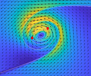
Another striking phenomenon one can observe is the formation of recirculation regions that, when the spiral begins to turn, are strong enough to create reverse flows (on the upper part of the layer to the left of the core, and on the lower part of the layer to the right of the core), see figure 4(a). These reverse flows, which cause the flow above and below the curve to have the same direction, weaken the jump across the curve, so that the vorticity $\omega _{\mathcal {C}}$ develops two minima. In figures 4(a)–4(c), these minima are marked with red dots; with ($\times$) we have marked the stagnation point, where the flow reverses its direction to the left of the core. The stagnation point to the right of the core, not visible in the figures, is close to the upper-right corner of the figures. These stagnation points separate the arms of the spiral from the inner part of the spiral: all the vorticity between these stagnation points is convected toward the core of the spiral. Between the two minima, vorticity reaches, at the centre of the spiral, a peak. This is visible in figure 5(b), where we plot, at different times, the vorticity $\omega _{\mathcal {C}}$ in terms of the arc length $s$ of $\mathcal {C}$.

Figure 4. The kinetic energy density ($|\boldsymbol {u}|^2/2$) for $Re=2\times 10^4$ at various times: (a) at $t=2.4$; (b) at $t=2.875$; (c) at $t=4.2$. The arrows represent the velocity $\boldsymbol {u}$, the red points are the points of minimal vorticity on the central curve $\mathcal {C}$, the red symbol $\times$ signals the point of minimal kinetic energy on the layer outside the core.

Figure 5. The vorticity $\omega _{\mathcal {C}}(s)$ on the material curve at different times for (a) $Re=10^{3}$ and (b) $Re=2\times 10^{4}$. The origin of $s$ is $(0,{\rm \pi} )$, and data are shown only for $s\geqslant 0$ (curve are extended by parity for $s<0$). For $Re=2\times 10^{4}$, at $t=2.4$, the transport of vorticity from the layer braid to the main core, leads to high values of the vorticity between the two minima. This phenomenon is also observable for $Re\geqslant 5\times 10^{3}$, but not for $Re=10^{3}$.

At $t=2.4$, that is when palinstrophy begins to increase, the peak of vorticity is reached at the centre of the core, delimited by the two local minima.

The above description of the layer motion in terms of palinstrophy growth replicates similar analyses already present in literature for different vorticity configurations (Ayala & Protas Reference Ayala and Protas2014; Kimura & Herring Reference Kimura and Herring2001). In the geophysical literature the study of the palinstrophy has been shown to be a useful tool to understand vorticity evolution during extreme events, see Schubert et al. (Reference Schubert, Montgomery, Taft, Guinn, Fulton, Kossin and Edwards1999) and Abarca & Corbosiero (Reference Abarca and Corbosiero2005).

2.2.3. Low-$Re$ regime

In the low-$Re$ regime, as opposed to the moderate- to high-$Re$ regime, we have observed neither mixing events nor palinstrophy growth. In figure 2(e,f), we can see that the roll-up process is also accompanied by the formation of local maxima in the palinstrophy density in the braids in the vicinity of the cores. In this case, compared with the moderate- to high-$Re$ regime, the flow evolution is characterized simply by the large-scale motion of the two symmetric cores. Moreover, due to high dissipative effects, the two cores are very weak, and they are not strong enough to produce significant stretching of the braids. Consequently, the palinstrophy density is always low (of the order of $10^2$ and $10^3$ in the braid), whereas palinstrophy $\mathcal {P}(t)$ never increases, see figure 3. For low $Re$ one never sees the formation of the minimum of $\omega _\mathcal {C}$ on the left of the maximum (see figure 5a), an event that, instead, characterizes the moderate- to high-$Re$ regime. The final significant event is the merging of the two cores, visible in figure 2(c).

From the analysis of the previous subsections 2.2.2 and 2.2.3, one can conclude that, in both cases, the linear Kelvin–Helmholtz instability, which causes the roll-up of the layer, rules the initial stages of the dynamics. The subsequent stages are determined by the competition between viscous dissipation and stretching, see (2.14) and (2.15), which is a fully nonlinear phenomenon. For lower $Re$, dissipation dominates, palinstrophy decreases, and no small-scale phenomena appear. Increasing the $Re$, stretching dominates over dissipation and causes the growth of palinstrophy and vorticity gradients: small scales (that, in § 3, we shall interpret in terms of complex singularities) not damped by viscosity appear, ultimately evolving in the concentration of vorticity.

The analysis of the Fourier energy spectra gives further evidence to these phenomena and adds more meaning to them. We define the kinetic energy density $\mathcal {K}\equiv |\boldsymbol {u}|^2/2$ and, in figure 6(a,b), we show the 1D spectrum obtained from $\mathcal {K}$ through shell summation

(2.16)\begin{equation} A_K=\sum_{K\leqslant|(k_x,k_y)| < K+1}| \hat{\mathcal{K}}_{k_x,k_y}|,\quad K\geqslant0, \end{equation}

where $\hat {\mathcal {K}}_{k_x,k_y}$ are the Fourier modes of $\mathcal {K}$. In figure 6(a), one can note the appearance of a range of growing modes: these modes are intermediate between the range of small wavenumbers (related to the large-scale feature of the fluid motion) and the range of large wavenumbers (very small scales, within the dissipative range). The growth of the intermediate modes coincides with the palinstrophy growth phase. Therefore, it is not observable for $Re<5\times 10^3$, that is, when dissipation dominates, it is barely visible for $Re=5\times 10^3$, and clearly noticeable for $Re\geqslant 10^4$.

Figure 6. (a) Energy density spectrum for $Re=2\times 10^4$ at different times. A range of growing uncoupled modes emerge during the palinstrophy growth phase. (b) Energy density spectrum for various $Re$ at the time of palinstrophy peak. In the inset the spectrum for $Re=10^3$ for which no growing range is observed. (c) The most excited mode $K_e$ in the uncoupled range vs the $Re^{1/2}$, and the best power-law fitting curve.

The appearance of the above-described range of excited modes is related to the appearance of the $O(Re^{-1/2})$ structure, that is, the core that forms due to intense stretching and fast rotation. In fact, the most excited wavenumber ${K_e}$ in this range, measured at the time of the palinstrophy peak, follows quite well the law ${K_e}\approx 0.42Re^{1/2}$, as shown in figure 6(c). The excitation of the intermediate modes, therefore, is another sign of the bifurcation occurring at approximately $Re \approx 5\times 10^3$.

The phenomena we have encountered in this section, such as palinstrophy growth and the excitation of the intermediate range of modes, are observed, during transition regimes, in flows ruled by very different mechanisms, such as boundary layers, mixing layers and jet flows. For instance, in boundary layer flows, the palinstrophy grows during the transition to the small-scale regime, which governs the interactions between the boundary layer and the inviscid outer flow for large enough $Re$ numbers (Gargano, Sammartino & Sciacca Reference Gargano, Sammartino and Sciacca2011; Gargano et al. Reference Gargano, Sammartino, Sciacca and Cassel2014). This transition, as shown in Nguyen Van Yen et al. (Reference Nguyen Van Yen, Waidmann, Klein, Farge and Schneider2018), appears to be related to the instabilities forming in the reversed flow region near the wall; the range of unstable wavenumbers scales as $Re^{1/2}$. In mixing layers and jet flows (Catrakis & Dimotakis Reference Catrakis and Dimotakis1996; Dimotakis Reference Dimotakis2000; Cook & Dimotakis Reference Cook and Dimotakis2001; Dimotakis Reference Dimotakis2005), the transition to turbulence is accompanied by the formation of large vorticity gradients, along with a typical energy spectrum behaviour: the mechanism of decoupling of the inner scales (viscously damped) from the outer scales (characterizing the large-scale motion), responsible for the transition to turbulence is the same we have encountered in analysing the energy spectrum of the vortex layers.

No vorticity is generated during the vortex layers’ evolution, contrary to what is quintessential of the boundary layer dynamics. Moreover, vortex layers do not evolve in turbulent flows, as it happens for mixing layers. Nevertheless, we have seen that all these configurations show striking similarities; among them, we also mention the existence of a Reynolds number bifurcation value, in all cases laying between $5\times 10^3$ and $10^4$. All this suggests the existence of a common mechanism of competition between dissipation and vorticity gradients creation that, for high enough $Re$, triggers the transition toward states characterized by small scales excitation, mixing and vorticity concentration.

2.3. Vortex layer solution for $Re\rightarrow \infty$: self-similar behaviour

In this section, we shall compare the behaviours of the material curve $\mathcal {C}=(x(\theta ),y(\theta ))$ at different $Re$. In figure 7, the curve $\mathcal {C}$ is shown at time $t=4$ for increasing $Re$, starting from $Re=1000$. It is evident that outside the core of the spiral the various curves collapse onto a single curve, whereas inside the core the spirals are strongly dependent on the $Re$ number: the roll-up process is more intense for increasing $Re$, and, at a fixed time, the spiral contains more windings as $Re$ increases. On the other hand, one can see that once rescaled with $Re^{1/2}$, the curves inside the core coincide. In fact, we introduce the spatial scaling

(2.17a,b)\begin{equation} X_{Re}(\theta)=Re^{1/2}\left(x(\theta)-x_c\right),\quad Y_{Re}(\theta)=Re^{1/2}\left(y(\theta)-y_c\right), \end{equation}

where the point $(x_c,y_c)$ is the centre of the spiral, that is, the point of $\mathcal {C}$ with the highest vorticity. In figures 8(a) and 8(b), the scaled curves are shown when two and three windings have already formed, respectively. The winding of the spirals are defined as follows: we assume that the first winding begins when, for the first time, the tangent at $(x_c,y_c)$ is vertical, whereas the $(k+1)$th winding begins when the tangent at $(x_c,y_c)$ forms an angle of ${\rm \pi} /2+k{\rm \pi}$, $k\geqslant 0$, with the horizontal direction. For $Re\geqslant 5\times 10^3$, the rescaled curves collapse onto a single spiral, especially in the innermost part of the core. The fact that, instead, for $Re=10^3$, the scaled curve has an entirely different form, shows once again the separation between the two, low and moderate–high, $Re$ regimes.

Figure 7. The central curve $\mathcal {C}$ at $t=4$ for various $Re$. Outside the spiral region, all the curves collapse onto a single curve.

Figure 8. Self-similarity of the central curve inside the core. The spirals, rescaled as (2.17a,b), when two (a) and three (b) windings are formed. The times are $t\approx 6.48,3.74,3.16,2.74$ for (a) and $t\approx 7.98,4.25,3.5,2.98$ for (b).

Figure 9(a,b) shows the same comparison of figure 8, at the time in which the derivatives in the $x$ and $y$ direction, respectively, vanish, that is, when the first winding begins to form and when the curve has done half a turn. In figure 9(c), we report the times at which the above events occur, where it is evident that the spatial scaling (2.17a,b) should be complemented with the temporal scaling

(2.18)\begin{equation} T=Re^{1/3} (t-t_s), \end{equation}

where $t_s$ the singularity time for the BR equation.

Figure 9. (a) The rescaled curves at the beginning of the first winding when the $x$-derivative vanishes. (b) The rescaled curve when the $y$-derivative vanishes. (c) Plots in log–log scale of the times $t-t_s$ at which the first winding begins (vanishing of the $x$-derivative of $\mathcal {C}$) and when $\mathcal {C}$ does half a turn (vanishing of the $y$-derivative of $\mathcal {C}$), as function of the $Re$. Here $t_s=1.507$ is the time in which BR solution develops singularity. Both curves follow the time scaling $t-t_s\sim Re^{-1/3}$.

The above scaling suggests that in the limit $Re\rightarrow \infty$, the layer shrinks to a vortex-sheet curve satisfying, at $t\rightarrow t_s^{+}$, the conditions $\partial _\theta x,\partial _\theta y\rightarrow 0$ in its centre. This would imply the blow-up of the curvature $\kappa _\mathcal {C}(\theta,t)=(x_\theta y_{\theta \theta }- y_\theta x_{\theta \theta })/((x_\theta ^2+y_\theta ^2)^{3/2})$ and of the true vortex sheet strength

(2.19)\begin{equation} \hat{\gamma}_\mathcal{C}(\theta,t)\propto|(x_\theta,y_\theta)|^{{-}1}=|\partial_\theta s(\theta)|^{{-}1}, \end{equation}

where $\hat {\gamma }_\mathcal {C}(\theta,t)$ is classically interpreted as a measure of the circulation density.

In figure 10(a), we show the behaviour of $\kappa _\mathcal {C}$ for $Re=7.5\times 10^4$ at different times; one can observe how, at $t=1.9275$, the curvature has dramatically increased its maximum magnitude at two different points. These points are close to the centre of the spiral, and visible as empty black squares in figure 10(c). Figure 11(a), where we report, for different $Re$, the time evolution of $\textrm {max}_{\theta }|\kappa _\mathcal {C}|$, gives more support to the diverging behaviour at $t_s$ for $Re\rightarrow \infty$.

Figure 10. Singular-like behaviour of the central curve $\mathcal {C}$ for $Re=1.5\times 10^5$. (a) The behaviour, at different times, of the curvature $\kappa _\mathcal {C}$ of the central curve $\mathcal {C}$ for $Re=1.5\times 10^5$. At $t_{1w}=1.845$, the time at which the first winding begins, $\kappa _\mathcal {C}$ has dramatically increased its maximum magnitude in two different points, close to the centre of the spiral. (b) The behaviour, at different times, of $\hat {\gamma }_{\mathcal {C}}$ for $Re=1.5\times 10^5$. At $t_{1w}=1.845$, $\hat {\gamma }_{\mathcal {C}}$ has a spike in the centre of $\mathcal {C}$, and its maximum value significantly increases. (c) The curve $\mathcal {C}$ for $Re=1.5\times 10^5$ at different times. In the inset, the magnification. Black circles are points of maximum $\hat {\gamma }_{\mathcal {C}}$; empty black squares are points of maximum curvature $\kappa _\mathcal {C}$ which tend to collapse on the centre of the curve.

Figure 11. The time behaviour of the maxima of the curvature $\kappa _\mathcal {C}$ and vortex strength $\hat {\gamma }_{\mathcal {C}}$. (a) The maximum value of the curvature $\kappa _\mathcal {C}$ for various $Re$ up to the time in which the first winding forms in the layer. For increasing $Re$ this value rapidly increases after $t_s=1.507$, with $t_s$ being the singularity time for the vortex sheet solution of the BR equation. (b) The maximum value of $\hat {\gamma }_{\mathcal {C}}$ for various $Re$, up to the time in which the first derivative of the $x$-component vanishes. The maximum value is always reached in the centre of the curve, that is, the point having the highest vorticity $\omega _{\mathcal {C}}$. The black dotted horizontal line is the maximum value of the true vortex strength $\hat {\gamma }_{BR}$ computed from the BR-vortex sheet motion at the singularity time $t_s$.

For a vortex-sheet curve, the true vortex strength $\hat {\gamma }_\mathcal {C}$ is a well-defined quantity. Instead, for a viscous layer, at each point $s$ of $\mathcal {C}$, we measure the vortex layer strength $\hat {\gamma }_{\mathcal {C}}$ as the total vorticity integrated along the normal to the curve at that point. The roll-up of the layer limits the application of this procedure: we have found that we can obtain a reliable measure of $\hat {\gamma }_{\mathcal {C}}$ only up to the formation of the first winding. In figure 10(c), we show the behaviour of $\hat {\gamma }_{\mathcal {C}}$, for $Re=7.5\times 10^4$, at $t=1.507,1.75,1.9275$. In figure 11(b) we report, at different $Re$, the maximum values attained by $\hat {\gamma }_{\mathcal {C}}$, up to the time in which the first winding forms: it is evident that this value rapidly increases both with time and for larger $Re$, although the predicted diverging behaviour for $t\rightarrow t_s^{+}$ is less evident if compared with the eruptive behaviour of the maximum curvature $\textrm {max}_{\theta }\kappa _{\mathcal {C}}$. The point of $\mathcal {C}$ having the highest value of $\hat {\gamma }_{\mathcal {C}}$ is the centre of the spiral, and visible as a black circle in figure 10(c).

We also note that the net circulation of the core of the layer decreases for increasing $Re$. To measure the circulation of the core, we have adopted a procedure similar to that used in Baker & Shelley (Reference Baker and Shelley1990). In particular, we consider two material curves $\mathcal {C}_{{up}},\mathcal {C}_{{down}}$ consisting on particles initially placed at a distance $dRe^{-1/2}$ above and below the curve $\mathcal {C}$. The real positive parameter $d$ sets how distant $\mathcal {C}_{{up}}$ and $\mathcal {C}_{{down}}$ are from $\mathcal {C}$. The core of the layer at each time is then the region bounded by $\mathcal {C}_{{up}},\mathcal {C}_{{down}}$ on the one hand, and by the straight lines starting from the point of maximum curvature in $\mathcal {C}_{{up}}$ (or $\mathcal {C}_{{down}}$) and reaching the closest point in $\mathcal {C}_{{down}}$ (or $\mathcal {C}_{{up}}$) on the other. One can, therefore, compute the circulation of the core as the integral of the vorticity over this area. We have checked at several times, and for different values of $d$, that the circulation decreases for increasing $Re$, meaning that most of the vorticity is concentrated outside the core of the layer.

If the depicted trend continues in the limit $Re\rightarrow \infty$, the vortex layer tends to a vortex sheet curve with diverging curvature and true vortex strength, and zero circulation increment in its centre. This possible blow up implies also $\partial _\theta s(\theta )=0$, so that the flow particles coalesce in the centre of $\mathcal {C}$ where the true vortex strength becomes infinite. In that case, $\hat {\gamma }_\mathcal {C}$ is the true vortex strength defined on a vortex sheet curve, and goes like $|\partial _\theta s(\theta )|^{-1}$. Hence, the collision condition $\partial _\theta s(\theta )=0$ is satisfied only when the true vortex strength diverges. This structure is also consistent with the results shown in Baker & Shelley (Reference Baker and Shelley1990), where the authors found the same asymptotic behaviour in the zero-thickness limit of an inviscid vortex layer of uniform vorticity. A similar conclusion has been proposed also in DeVoria & Mohseni (Reference DeVoria and Mohseni2018) where the authors showed that the true vortex strength of an inviscid vortex sheet rapidly increases just after the singularity time of the BR solution.

The diverging behaviour of $\kappa _\mathcal {C}$ and $\hat \gamma _{\mathcal {C}}$ will receive further evidence from the singularity analysis we shall present in § 3.2.

3.1. Singularity tracking for the vorticity $\omega _{\mathcal {C}}$

We have already seen how the vorticity on the curve, $\omega _{\mathcal {C}}$, develops two minima (in the moderate- to high-$Re$ regime, whereas for low $Re$, there is only one minimum), which separate the inner from the outer core. These minima correspond to zones where the formation of sharp vorticity gradients occurs, with associated intense stretching of the curve. See the discussion after (2.15), where we explained how stretching and growth of vorticity gradients are closely related.

In figure 12(a), we show, for $Re=2\times 10^4$, $\omega _\mathcal {C}$ both as a function of $\theta$ and the arc length $s(\theta )$: the presence of the minima and sharp gradients is evident. The stretching of the curve is apparent in figure 12(b), where one can see that the function $s(\theta )$ increases (strongly, after time $t=2$) in correspondence with the minima of $\omega _\mathcal {C}$. It is also remarkable that, between the two stretching regions, there is a zone where $s(\theta )$ is almost flat, which implies that fluid particles that initially were well separated are almost coalescing.

Figure 12. (a) The vorticity $\omega _\mathcal {C}$ along the material curve $\mathcal {C}$ is shown as a function of both $\theta$ and $s(\theta )$ for $Re=2\times 10^4$ at $t=3$. In $s(\theta )$, high gradients form corresponding to the minima of $\omega _\mathcal {C}$, where the stretching of $\mathcal {C}$ is present. (b) Arc length of the curve $\mathcal {C}$ as a function of the parameter $\theta$ for $Re=2\times 10^4$ from $t=2$ to $t=3$ (time steps of $0.2$). The curve $\mathcal {C}$ is elongated close to the points where vorticity is transported from the layer braid to the core of the layer (see also figure 5b). In the centre of the core, where $s(\theta )$ is almost flat, a strong compression (coalescence of fluid particles) along the curve is present.

In this section, we show how the vorticity minima are related to the presence of complex singularities in $\omega _{\mathcal {C}}$, and how one can characterize the two flow regimes (low and moderate–high $Re$) in terms of the behaviour of the trajectory of the complex singularities.

We were able to detect and track in time, for all the $Re$ considered, two main singularities whose complex locations are denoted with $\theta ^{\omega _\mathcal {C}}_1=\theta _1+\textrm {i}\theta _{im_1}$ and $\theta ^{\omega _\mathcal {C}}_2=\theta _2+\textrm {i}\theta _{im_2}$ (from the symmetry of the problem there are also singularities at $2{\rm \pi} -\theta ^{\omega _\mathcal {C}}_1$ and $2{\rm \pi} -\theta ^{\omega _\mathcal {C}}_2$). Hereafter, we label these singularities (and all the singularities we introduce in the sequel) with their locations. These two singularities are indeed related to the minima in $\omega _\mathcal {C}$, as they have real components that correspond to the local minima visible, for instance, in figure 12(a) for $Re=2\times 10^4$.

To highlight the different behaviour of $\theta ^{\omega _\mathcal {C}}_1$ and $\theta ^{\omega _\mathcal {C}}_2$, we show in figures 13 the path of the singularities in the complex plane $(s(\theta ),\theta _{im})$. All the tracking start at $t=2$, up to $t=5.9$ for $Re=10^{3}$, up to $t=3.25$ for $Re=10^{4}$, and up to $t=2.85$ for $Re=2\times 10^{4}$: these final times are the time of formation of the third winding for $Re=10^{3}$ and the times in which palinstrophy has its local maximum ($Re=10^{4},2\times 10^{4}$), respectively. We can observe different behaviours depending on the $Re$ number, mainly in the position of $\theta ^{\omega _\mathcal {C}}_1$. In fact, for $Re=10^{4},2\times 10^{4}$ (and also for $Re=5\times 10^{3}$, not shown here), after an initial period in which the singularity moves toward the real plane having almost fixed real part $s(\textrm {Re}\{\theta ^{\omega _\mathcal {C}}_1\})$, during the mixing events $\theta ^{\omega _\mathcal {C}}_1$ begins to rapidly shift on the right along $s$ and to move toward the second singularity $\theta ^{\omega _\mathcal {C}}_2$. See also supplementary movie 2 where, for the case $Re=10^4$, we report the time evolution of the singularities in the complex plane and the corresponding vorticity evolution: red and black dots in the central curve are the points corresponding to the real parts of the singularities. When $\theta ^{\omega _\mathcal {C}}_1$ is sufficiently close to the real domain, the local minimum visible, for instance, in figure 5(b) forms.

Figure 13. Tracking the singularities $\theta ^{\omega _\mathcal {C}}_1$ (a) and $\theta ^{\omega _\mathcal {C}}_2$ (b) for various $Re$ in the complex plane $(s(\theta ),\theta _{im})$ (see supplementary movie 2 for the case $Re=10^4$). The blue dot is for time $t=2.4$, red dot is for time $t=2.7$, green dot is $t=2.85$. All the tracking starts from $t=2$, up to $t=5.9$ for $Re=10^{3}$, to $t=3.25$ for $Re=10^{4}$, and up to $t=2.85$ for $Re=2\times 10^{4}$. These final times are, respectively, the time of formation of the third winding for $Re=10^{3}$, and the times at which palinstrophy has its local maximum for $Re=10^{4},2\times 10^{4}$.

On the other hand, in the case $Re=10^{3}$, $\theta ^{\omega _\mathcal {C}}_1$ always moves leftward along $s$. At $t\approx 5.9$, that is when the third winding forms in $\mathcal {C}$, $\theta ^{\omega _\mathcal {C}}_1$ collapses to $s(0)=0$ with the symmetric singularity $2{\rm \pi} -\theta ^{\omega _\mathcal {C}}_1$. As already stated in the previous section, no mixing events are observed for $Re=10^{3}$, no new local minimum for $\omega _\mathcal {C}$ on the left of the maximum and, from the point of view of the complex singularity $\theta ^{\omega _\mathcal {C}}_1$ always moves toward the origin $s=0$ and never moves toward the second singularity $\theta ^{\omega _\mathcal {C}}_2$.

In the qualitative behaviour of $\theta ^{\omega _{\mathcal {C}}}_2$, we observe no difference related to $Re$: in all $Re$ regimes, initially, $\theta ^{\omega _\mathcal {C}}_2$ moves toward the real domain slightly shifting leftward along $s$, then goes rightward, still approaching the real axis, see figure 13(b).

Therefore, $\theta ^{\omega _\mathcal {C}}_1$ plays the key role in the formation of the intense mixing and the concentration phenomena occurring for higher $Re$: $\theta ^{\omega _\mathcal {C}}_1$ is responsible for the extreme stretching of the curve and, ultimately, for the palinstrophy growth; moreover, the collision of $\theta ^{\omega _\mathcal {C}}_1$ with the other singularity $\theta ^{\omega _\mathcal {C}}_2$ causes, in the limit $Re\rightarrow \infty$, the blow-up of $\hat {\gamma }_\mathcal {C}$, a phenomenon which is absent in the BR dynamics.

Using the BPH method, we have determined the algebraic characters of the singularities. Usually, it is more difficult to determine the algebraic character of a singularity rather than its position (see, e.g., Caflisch et al. Reference Caflisch, Gargano, Sammartino and Sciacca2015). However, after time $t\geqslant 1.3$, the characters $\mu _{\theta ^{\omega _\mathcal {C}}_1}$ and $\mu _{\theta ^{\omega _\mathcal {C}}_2}$ of $\theta ^{\omega _\mathcal {C}}_1$ and $\theta ^{\omega _\mathcal {C}}_2$ have been reliably determined. For all $Re>10^3$, $\mu _{\theta ^{\omega _\mathcal {C}}_1}$ and $\mu _{\theta ^{\omega _\mathcal {C}}_1}$ are approximately equal to $1/2$, whereas, for $Re=10^3$, they have higher values, close to $0.9$, see table 1. The values $\mu _{\theta ^{\omega _\mathcal {C}}_1}$ and $\mu _{\theta ^{\omega _\mathcal {C}}_2}$ reveal that $\theta ^{\omega _\mathcal {C}}_1$ and $\theta ^{\omega _\mathcal {C}}_2$ are two branch points, consistent with the rapid variation of the first derivative of $\omega _{\mathcal {C}}$ close to its two local minima, see figure 12(b).

Table 1. Characters of the singularities at $t_s=1.507$. For each $Re$ we show the characters of the singularities: the vorticity $\omega _{\mathcal {C}}$, $\theta ^{\omega _\mathcal {C}}_{1,2}$; $(X_\mathcal {C},Y_\mathcal {C})$ in (4.7), $\theta _{1,2}^{X_\mathcal {C}}$ and $\theta _{1,2}^{Y_\mathcal {C}}$; the curvature $\kappa _{\mathcal {C}}$ of $\mathcal {C}$, $\theta _{1,2}^{\kappa _\mathcal {C}}$; and the vortex strength $\hat {\gamma }_{\mathcal {C}}$, $\theta ^{\hat {\gamma }_{\mathcal {C}}}$. Error bars are, in general, less than $15\,\%$ of the estimated parameters, except for the case $Re=10^3$, for which $\mu _{\theta ^{\hat {\gamma }_{\mathcal {C}}}},\mu _{\theta _{1,2}^{\kappa _\mathcal {C}}}$ have errors are up to the order of $80\,\%$ of the estimated parameters.

3.2. Singularity tracking for $\kappa _{\mathcal {C}}$ and $\hat {\gamma }_{\mathcal {C}}$

In § 2, we have seen that the final structure of the layer in the limit $Re\rightarrow \infty$ could be represented by a curve having, at $t_s=1.507$, the singularity time of the BR solution, infinite curvature and infinite true vortex strength. We show that the possible diverging nature of both $\kappa _{\mathcal {C}}$ and $\hat {\gamma }_{\mathcal {C}}$ is confirmed by the presence of complex singularities having negative character.

The explicit expression of the curvature of the material curve $\mathcal {C}$ is $\kappa _{\mathcal {C}}(\theta,t)=(x_\theta y_{\theta \theta }- y_\theta x_{\theta \theta })/((x_\theta ^2+y_\theta ^2)^{3/2})$. For all the $Re$ numbers considered, we have detected the presence of two complex singularities, $\theta _1^{\kappa _{\mathcal {C}}}$ and $\theta _2^{\kappa _\mathcal {C}}$. In figure 14(a), we represent the singularities in the complex plane $(\theta,\theta _{im})$, for different $Re$, at $t_s=1.507$ and at $t_{1w}$ the time when the first winding forms in $\mathcal {C}$.

Figure 14. (a) Tracking in the complex plane $(\theta,\theta _{im})$ of the two main singularities $\theta _{1,2}^{\kappa _\mathcal {C}}$ of the curvature $\kappa _\mathcal {C}$ of $\mathcal {C}$. Singularities are tracked at $t_s=1.507$ and at the time $t_{1w}$ in which the first winding forms (times reported in the text and in figure 10(a) for $Re=5\times 10^3, 10^4, 2\times 10^4, 7.5\times 10^4$ and $1.5\times 10^5$). The size of the markers decreases for larger $Re$. The value $\theta =1.287$, where the BR singularity forms, is also shown as a straight line. (b) Tracking in the complex plane $(\theta,\theta _{im})$ of the main singularity $\theta ^{\hat {\gamma }_{\mathcal {C}}}$ of the vortex strength $\hat {\gamma }_{\mathcal {C}}$. The singularity is tracked at $t_s=1.507$ and at the time $t_{1w}$ in which the first winding forms for $Re=5\times 10^3, 10^4, 2\times 10^4, 7.5\times 10^4$ and $1.5\times 10^5$. The size of the markers decreases for larger $Re$. (c,d) Imaginary parts of the singularities shown in (a,b) versus the $Re$ number and best power-law fitting (log–log scale).

The singularities $\theta _1^{\kappa _\mathcal {C}}$ and $\theta _2^{\kappa _\mathcal {C}}$ have different positions than those of $\omega _\mathcal {C}$, although some similarities are evident. They are closer to the real domain for increasing $Re$, and they tend to coalesce. In figure 14(c) we show a consistent power-law scaling $\theta _{im}\propto Re^{c}$, with $c=-0.17$ and $-0.16$ for the first and second singularities, respectively. This suggests that the singularities approach the real axis as $Re\rightarrow \infty$. (We have obtained a slightly more consistent fitting with a curve of the kind $\propto \log ^d(Re) Re^{c}$, although $d$ is a very small parameter of order $10^{-3}$). One can see the effects owing to the presence of these singularities in figure 10(b), where the two maximum curvature points (positive and negative) are located close to $s(\textrm {Re}\{{\theta _1^{\kappa _\mathcal {C}}}\})\approx 1.048$ and $s(\textrm {Re}\{{\theta _2^{\kappa _\mathcal {C}}}\})\approx 1.065$. Concerning the evaluation of the algebraic characters $\mu _{\theta _1^{\kappa _{\mathcal {C}}}}$ and $\mu _{\theta _2^{\kappa _\mathcal {C}}}$, we have found that both singularities have negative character at $t_s=1.507$ (see table 1) and $t_{1w}=1.9275$. The above analysis confirms that the limiting $Re\rightarrow \infty$ behaviour of $\mathcal {C}$, as far as the curvature is concerned, is entirely consistent with the behaviour observed in the BR solution. We note that the BPH method can find other complex singularities that are due to subsequent maximum points of curvature forming during the roll-up process. However, these secondary singularities are, in general, more distant from the real axis, and do not play a significant role in our analysis.

The singularity analysis of the vortex strength $\hat {\gamma }_{\mathcal {C}}$ reveals the presence of one main singularity, denoted by $\theta ^{\widehat {\gamma _{\mathcal {C}}}}$, and reported in figure 14(b), for different $Re$, and at times $t_s$ and $t_{1w}$. The presence of $\theta ^{\widehat {\gamma _{\mathcal {C}}}}$ can be related to the peak in $\hat {\gamma }_{\mathcal {C}}$ visible, for instance, in figure 10(b) in the centre of the spiral. At $t_s=1.507$, the singularity is quite far from the real axis ($\theta ^{\hat {\gamma }_{\mathcal {C}}}\approx 1.222+\textrm {i}0.41$), and the peak has a moderate magnitude. At $t_{1w}=1.937$, the singularity is closer to the real axis ($\theta ^{\hat {\gamma }_{\mathcal {C}}}\approx 1.233+\textrm {i}0.104$), and the peak in $\hat {\gamma }_{\mathcal {C}}$ is more pronounced in $s(1.233)\approx 1.12$; see figure 10(b). Similarly to the other singularities we have analysed, $\theta ^{\hat {\gamma }_{\mathcal {C}}}$ gets closer to the real axis for increasing $Re$. The distance from the real axis of the singularities versus the $Re$ is shown in figure 14(d) along with the best power-law fitting curve of the kind $\theta _{im}\propto Re^{c}$, with $c\approx -0.15$. The character $\mu _{\theta ^{\hat {\gamma }_{\mathcal {C}}}}$ of $\theta ^{\hat {\gamma }_{\mathcal {C}}}$ is negative (of order $\approx -0.4$) for the times we have considered, and for the moderate- to high-$Re$ regime; see table 1 at $t_s$. Given that our simulation indicate that $\textrm {Im}\{\theta ^{\hat {\gamma }_{\mathcal {C}}}\}\rightarrow 0$ when $Re\rightarrow \infty$, the above singularity analysis gives further evidence for the diverging behaviour of $\hat {\gamma }_{\mathcal {C}}$ for $t\rightarrow t_s^+$, as conjectured in § 2.3.

As reported in Appendix A, one recovers the characteristics of the singularities discussed previously through fitting procedures of the solution spectra. These procedures, unavoidably, are prone to errors. Concerning the character of the singularities, which is the most delicate quantity to be estimated, for $R\geqslant 5\times 10^3$, the amplitude of the confidence interval is $15\,\%$ for $95\,\%$ confidence level. Moreover, the goodness of the fitting model is attested by values of the $R^2$ coefficient very close to 1, typically between $0.98$ and $0.99$. For $Re=10^3$, we have obtained larger errors, especially for the characters: this is likely due to the large distance of the singularities from the real domain, making the noise-free part of the solution spectrum smaller as compared with the other cases, and governed mainly by the exponential decay, see (A1). For instance, for $Re=10^3$, we have obtained $\theta ^{\hat {\gamma }_{\mathcal {C}}}\approx 0.1\pm 0.09$; whereas, for $Re=10^4$, $\theta ^{\hat {\gamma }_{\mathcal {C}}}\approx -0.34\pm 0.025$. Moreover, the relative error decreases for increasing $Re$. Therefore, these errors do not affect the main conclusion of the present section, that is, $\hat {\gamma }_{\mathcal {C}}\rightarrow \infty$ for $Re\rightarrow \infty$.

4.1. The BR model

The initial vortex sheet corresponding to the vortex layer configuration that we have studied in previous sections consists of a vorticity distribution concentrated, as a delta function, on the curve

(4.1a,b)\begin{equation} \boldsymbol{x}_{BR}(\theta)=(\theta,{L_y}\sin({2{\rm \pi}\theta}/{L_x})/{4{\rm \pi}}), \quad \theta\in[{-}L_x/2,L_x/2], \end{equation}

with intensity

(4.2)\begin{equation} \gamma(\theta)=1. \end{equation}

The vorticity distribution has to be considered in the box $D=[-L_x/2,L_x/2]\times [-L_y/2,L_y/2]$ and extended by periodicity both in the $x$ and in the $y$ directions. Being $\gamma (\theta )=1$, the parameter $\theta$ identifies with the circulation $\varGamma =\int _0^{\theta }\gamma (\tilde \theta )\,\textrm {d}\tilde \theta$. Therefore, to compute the dynamics of the sheet, we use $\theta$ as a Lagrangian parameter, whereas the true vortex strength along the sheet is given by $\hat {\gamma }(\theta,t)=\gamma (\theta )|\partial _{\theta }\boldsymbol {x}_{BR}|^{-1}$. The choice of the Lagrangian parameter $\theta$ allows the evolution of the curve to be written without involving the equation for the true vortex strength $\hat {\gamma }(\theta,t)$ (see the interesting discussion in Lopes Filho, Nussenzveig Lopes & Shochet (Reference Lopes Filho, Nussenzveig Lopes and Shochet2007)). The BR equation hence reads as

(4.3)\begin{equation} \frac{\partial \boldsymbol{x}_{BR}(\theta,t)}{\partial t}=\int_{{-}L_x/2}^{L_x/2}{\boldsymbol{K}}_{L_x,L_y}(\boldsymbol{x}_{BR}(\theta,t)-\boldsymbol{x}_{BR}(\tilde{\theta},t)))\,\textrm{d}\tilde \theta, \end{equation}

where the components of the singular kernel are

(4.4)\begin{align} \boldsymbol{K}_{L_x,L_y}(\boldsymbol{x})&= \left(\frac{y}{L_xL_y}-\frac{1}{2L_x}\sum_{h={-}\infty}^{h=\infty}\frac{\sinh(2{\rm \pi} (y-hL_y)/L_x)}{\cosh(2{\rm \pi} (y-hL_y)/L_x)-\cos(2{\rm \pi} x/L_x)},\right.\nonumber\\ &\qquad \left.\frac{1}{2L_x}\sum_{h={-}\infty}^{h=\infty}\frac{\sin(2{\rm \pi} x/L_x)}{\cosh(2{\rm \pi} (y-hL_y)/L_x)-\cos(2{\rm \pi} x/L_x)}\right). \end{align}

One can obtain the above expression taking the orthogonal gradient of the fundamental solution of the 2D periodic Poisson equation, derived in Bailey et al. (Reference Bailey, Borwein, Crandall and Zucker2013).

To continue the solution after the singularity time, one can regularize the kernel with the classical vortex-blob method: see Krasny (Reference Krasny1986a), Cowley et al. (Reference Cowley, Baker and Tanveer1999) and Baker & Pham (Reference Baker and Pham2006). We have accomplished this by using the regularization reported in Baker & Pham (Reference Baker and Pham2006); see, in particular, their (2.8a) and (2.8b). In our case the regularized $\delta$–BR equation reads as

(4.5)\begin{equation} \frac{\partial \boldsymbol{x}_{BR}^{\delta}(\theta,t)}{\partial t}=\int_{{-}L_x/2}^{L_x/2}\boldsymbol{K}^{\delta}_{L_x,L_y}(\boldsymbol{x}_{BR}^{\delta}( \theta,t)-\boldsymbol{x}_{BR}^{\delta}(\tilde{\theta},t)))\,\textrm{d}\tilde{\theta}, \end{equation}

where the regularized kernel is

(4.6)\begin{align} &\boldsymbol{K}^{\delta}_{L_x,L_y}(\boldsymbol{x})\nonumber\\ &\quad =\left(\frac{y}{L_xL_y}-\frac{1}{2L_x}\sum_{h={-}\infty}^{h=\infty} \frac{y-hL_y}{\sqrt{(y-hL_y)^2+\delta^2}}\frac{\sinh(2{\rm \pi} \sqrt{(y-hL_y)^2+\delta^2}/L_x)}{\cosh(2{\rm \pi} \sqrt{(y-hL_y)^2+\delta^2}/L_x)-\cos(2{\rm \pi} x/L_x)},\right.\nonumber\\ &\qquad \left. \frac{1}{2L_x}\sum_{h={-}\infty}^{h=\infty}\frac{\sin(2{\rm \pi} x/L_x)}{\cosh(2{\rm \pi} \sqrt{(y-hL_y)^2+\delta^2}/L_x)-\cos(2{\rm \pi} x/L_x)}\right), \end{align}

and $\delta >0$ is the regularizing parameter. To solve the BR equation, we have used a fourth-order Runge–Kutta scheme; in (4.3) and (4.5), we have performed the integration by using the alternating points quadrature formula (see Krasny Reference Krasny1986a). Close to the singularity time, we had to use 65 536 discretization points. To avoid the growth of the round-off disturbances due to the Kelvin–Helmholtz instability, we apply the Fourier filtering technique (Krasny Reference Krasny1986b; Ely & Baker Reference Ely and Baker1993; Baker & Xie Reference Baker and Xie2011): performing computations with 32-digit precision, at each time step, we set to zero the Fourier modes with amplitude smaller than the threshold value $10^{-29}$. In the regularized case, filtering was necessary only for the case $\delta =10^{-3}$; a larger regularization is able to damp round-off. Finally, we need to evaluate only a finite number of terms in the infinite sums of (4.4) and (4.6), as they rapidly decay to zero with $h$; the choice $h=50$ was enough to ensure an error below the machine precision. In all the numerical simulations, we set $L_x=L_y=2{\rm \pi}$.

4.1.1. Comparison between the BR vortex sheet and the NS vortex layer singularities

In this section, we compare the outcomes of the singularity analysis for $\mathcal {C}$ (the centre of the layer), presented in § 3.2, with those coming from the BR solution's singularity analysis. In particular, we compare the singularities of the components of the $BR$ solution and $\mathcal {C}$, of the curvatures $\kappa _{BR}$ and $\kappa _\mathcal {C}$, and of the true vortex strengths $\hat {\gamma }_{BR}$ and $\hat {\gamma }_{\mathcal {C}}$. This comparison can be made only up to the time $t_s$ when the BR solution becomes singular.

In Caflisch et al. (Reference Caflisch, Gargano, Sammartino and Sciacca2017), the singularity analysis of $(X_{BR}(\theta,t), Y_{BR}(\theta,t))$, revealed that a singularity forms in a finite time. In particular, the two functions $X_{BR}(\theta,t), Y_{BR}(\theta,t)$ become singular at $t_s\approx 1.507$ and $\theta ^*\approx 1.287$. The singularities of $X_{BR}$ and $Y_{BR}$ always have the same positions in the complex plane, although they have different characterizations, $\mu _{X_{BR}}\approx 1.61$ and $\mu _{Y_{BR}}\approx 1.72$, respectively. Therefore, both components experience a blow-up in their second derivative, and the $X$-component is more singular than the $Y$-component. In figure 15, we show the trajectories of these singularities in the complexified $\theta$-plane. At $t=t_s$, the trajectory terminates, hitting the real axis and producing the blow-up of the solution. At $t=t_s$, also the curvature $\kappa _{BR}$ and the true vortex strength $\hat {\gamma }_{BR}$ become singular, with characterizations $\mu _{\kappa _{BR}}\approx -0.44$ and $\mu _{\hat \gamma _{BR}}\approx 0.55$, respectively. Therefore, at $\theta =\theta ^*$, the curvature diverges, whereas $\hat \gamma _{BR}$ has a cusp behaviour: at $t=t_s$, $\hat \gamma _{BR}$ is singular but finite. The above results are in full agreement with those predicted in Moore (Reference Moore1979), and later observed by other authors investigating numerically the singularities generated by vortex-sheet motion with several initial configurations (see, e.g. Krasny Reference Krasny1986b; Shelley Reference Shelley1992).

Figure 15. Trajectories of the two complex singularities $\theta _1^{X_\mathcal {C}}$ and $\theta _2^{X_\mathcal {C}}$ of the component $X_{\mathcal {C}}$ of the material curve $\mathcal {C}$. The tracking goes from $t=0.8$ up to $t_s=1.507$. The singularities of $Y_{\mathcal {C}}$ have similar trajectories. The dashed line is the tracking of the BR singularity. At $t_s$, the BR singularity, with character $3/2$, hits the real axis. At $t_s$, the characters of $\theta _1^{X_\mathcal {C}}$ and $\theta _2^{X_\mathcal {C}}$ are compatible with the character of the BR solution; see table 1.

In figure 16, we show the vortex sheet curve and its curvature, and compare them with the $\mathcal {C}$ curve (the centre of the vortex layer) and its curvature. The time is $t=1.505$, just before the singularity formation. The $\mathcal {C}$ curve approximates the vortex sheet curve well; the effect of the regularization is evident in the smooth behaviour of the curvature of $\mathcal {C}$.

Figure 16. (a) The vortex sheet curve obtained solving the BR equation, at $t=1.505$, and the curve $\mathcal {C}$, for various $Re$, at the same time. (b) The curvatures $\kappa _{BR}$ and $\kappa _{\mathcal {C}}$, at $t=1.505$.

Given the parametrization $\mathcal {C}=(x(\theta,t),y(\theta,t))$, we apply the BPH method to find the singularities of the components

(4.7)\begin{equation} (X_{\mathcal{C}}(\theta,t),Y_{\mathcal{C}}(\theta,t))=(x(\theta,t)-\theta,y(\theta,t)), \quad \theta \in [-{\rm \pi},{\rm \pi}].\end{equation}

We label these singularities $\theta _1^{X_\mathcal {C}},\theta _2^{X_\mathcal {C}}$ and $\theta _1^{Y_\mathcal {C}},\theta _2^{Y_\mathcal {C}}$. As one could expect, the positions of the singularities of $X_{\mathcal {C}}$ and $Y_{\mathcal {C}}$ in the complex plane coincide with those of $\omega _\mathcal {C}$ and are shown, for instance, in figures 13. In figure 15 we show the paths in the complex plane of $\theta _1^{X_\mathcal {C}}$ and $\theta _2^{X_\mathcal {C}}$ ($\theta _1^{Y_\mathcal {C}},\theta _2^{Y_\mathcal {C}}$ have the same positions) for various $Re$. The paths are represented up to the singularity time of the BR solution $t_s=1.507$. As $Re$ increases, the singularities are closer to the real axis, and the distance between $\theta _1^{X_\mathcal {C}}$ and $\theta _2^{X_\mathcal {C}}$ diminishes; moreover, they seem to converge toward the BR singularity. We have found that, at time $t_s=1.507$, both singularities have characters $\mu _{\theta _{1,2}^{X_\mathcal {C}}}$ and $\mu _{\theta _{1,2}^{Y_\mathcal {C}}}$ in the range (1.0–1.5), compatible with the predicted characterization of the BR singularity (see table 1) and with the blow-up in their second derivatives. At subsequent times, for instance at $t_{1w}$, these characters remain in the same range.

A similar behaviour is observed for the singularities of the curvature: the curvature of $\mathcal {C}$ admits two singularities (see § 3.2) that, in the limit $Re\rightarrow \infty$, seem to converge toward the BR curvature singularity. The algebraic characters of these singularities appear to be the same; see the last three columns of table 1.

The crucial difference between the vortex sheet and $\mathcal {C}$ lies in the singularity of the true vortex strengths $\hat {\gamma }_{BR}$ and $\hat {\gamma }_{\mathcal {C}}$ (the differences between the characters of the singularities are reported in table 3). In the BR case, at $t_s$, a cusp forms in $\hat {\gamma }_{BR}$ and $\partial _\theta s(\theta )$ is small but not vanishing. In contrast, in the analysis we have performed in § 3.2, we found that $\hat {\gamma }_{\mathcal {C}}$ has a singularity with negative algebraic character $\mu _{\theta ^{\hat {\gamma }_{\mathcal {C}}}}$ (of order $\approx -1/3$, see table 1). This means that, in the limit $Re\rightarrow \infty$ and at $t_s$, $\hat {\gamma }_{\mathcal {C}}$ blows up. One of the consequences is that $\partial _\theta s(\theta )=0$ and, therefore, an infinite particle compression occurs at the centre of the spiral, with the two vorticity minima colliding. The difference between the behaviour of the BR solution at $t=t_s$, and the infinite Reynolds number of the vortex layer solution, suggests that BR, close to the singularity, is not the zero-viscosity limit of the NS vortex layer solutions.

4.2. Vortex blob regularization

In this section, we shall compare the solutions of the $\delta$–BR equation with the NS vortex layer solution.

In figure 17(a), we show the comparison between the curves $\mathcal {C}$, the centre of the NS layer, and $\boldsymbol {x}^\delta _{BR}$, the solution of the $\delta$–BR equation; the solutions are computed taking $Re=10^4$ and $\delta =10^{-2}$, respectively. The two curves overlap in the outer part of the spiral while one can appreciate significant qualitative differences in the innermost part of the spiral, as the curve $\boldsymbol {x}^\delta _ {BR}$ develops more turns.

Figure 17. (a) Plot of $\mathcal {C}$, the NS (with $Re=10^4$) layer's central curve, and the vortex sheet obtained from the $\delta$-vortex blob regularization (with $\delta =10^{-2}$). The times are $t=2$, $t=3.0$ and $t=3.6$ (upper plots): the outer part of the spirals seems to be independent of the regularization used, whereas the innermost part depends on it. In the inset, the magnification of the spirals at $t=3.6$. (b) We show the spirals after the scaling (4.8) for $\delta =10^{-1},10^{-2},10^{-3}$. $(c)$ We compare the spiral given by the $\delta$–BR solution (scaled by (4.8)) with the material curve $\mathcal {C}$ (in the NS and Euler cases). The regularizing parameters are $\delta =10^{-3}$ for the $\delta$ model, $Re=2\times 10^{4}$ for the viscous layer and $\delta =0.0141$ for the inviscid layer.

We have seen that the inner part of the spiral formed by $\mathcal {C}$ obeys a self-similarity law given by (2.17a,b). It is also known that a similar scaling exists for the vortex blob regularization; Baker & Pham (Reference Baker and Pham2006) and Sohn (Reference Sohn2014) showed that the inner core region of the spirals is invariant under the transformation

(4.8)\begin{equation} \textbf{X}_{\delta}=\left(\boldsymbol{x}_{BR}^\delta-(x_c,y_c)\right)/\delta. \end{equation}

The self-similarity law is illustrated in figure 17(b). Formally (4.8) is the same as the $Re^{-1/2}$-scaling (2.17a,b) for the curve $\mathcal {C}$.

In figure 17(c), we compare the rescaled $\mathcal {C}$ and the rescaled $\delta$–BR curves when they have completed the same number of turns. The figure shows an almost perfect matching in the very vicinity of the centre. This comparison shows that both the regularizations predict a qualitatively similar structure represented by the spiral. However, the differences obtained from the scaled curves highlight some quantitative differences, which does not rule out the possibility that, in the limits $\delta \rightarrow 0,Re\rightarrow \infty$, the two regularizations provide different weak solutions of the Euler equations. We have analysed the outcomes of the singularity analysis for the components

(4.9)\begin{equation} (X^{\delta}_{BR}(\theta,t),Y^{\delta}_{BR}(\theta,t))=(x_{BR}^\delta(\theta,t)-\theta,{y}_{BR}^\delta(\theta,t)), \quad \theta \in [-{\rm \pi},{\rm \pi}].\end{equation}

and compared with the $\mathcal {C}$ case. Similarly to $\mathcal {C}$, both components have two main singularities $\theta _{1,2}^{X_{BR}^\delta }$ and $\theta _{1,2}^{Y^\delta _{BR}}$. Figure 18 reports the paths of $\theta _{1,2}^{X_{BR}^\delta }$ in the complex plane. For $\delta =10^{-3}$, the singularities are very close to each other, and the BPH method does not discern the positions of the two singularities. Compared with the tracking of the singularities of $\mathcal {C}$ in figure 15, the $\theta _{1,2}^{X^\delta _{BR}}$ are, in general closer to the singularity of the BR solution and closer to the real domain: for instance, one can check this from the tracking in the case when $\delta =Re^{-1/2}=10^{-2}$. The characterization of the vorticity intensity singularity $\theta ^{\hat {\gamma }_{\delta }}$ is the most relevant quantity. From table 2 one can see that the algebraic character of $\theta ^{\hat {\gamma }_{\delta }}$ is $\mu _{\theta ^{\hat \gamma _\delta }}\approx -0.43$, which makes the vorticity concentration for the BR-$\delta$ stronger than for the NS-layer case, see table 1. The error bound in the fitting procedure is even smaller than in the viscous case, being, in general, of magnitude less than $10\,\%$ of the estimated values.

Figure 18. Tracking the complex singularities $\theta _1^{X^\delta _{BR}}$ and $\theta _2^{X^\delta _{BR}}$ of the component $X^\delta _{BR}$ of the regularized $\delta$–BR solution in the complex plane from $t=0.8$ up to $t_s=1.507$ . The singularities $\theta _1^{Y^\delta _{BR}}$ and $\theta _2^{Y^\delta _{BR}}$ of the $Y_{BR}^\delta$ components have the same tracking. The dashed line is the tracking of the BR singularity. For $\delta =10^{-3}$ the two singularities are very close to each other, $\theta _1^{X^\delta _{BR}}\approx \theta _2^{X^\delta _{BR}}$, so only one singularity is tracked. At $t = t_s$ the singularities have characters compatible with the singularity character of the BR solution (see table 2).

Table 2. Characters of the singularities of the $\delta$–BR solution at $t_s=1.507$. For each $\delta$ we show the characters of the singularities: of $(X^\delta _{BR},Y^\delta _{BR})$ in (4.9), $\mu _{\theta _{1,2}^{X_{BR}^\delta }}$ and $\mu _{\theta _{1,2}^{Y_{BR}^\delta }}$; of the curvature $\kappa _\delta$, $\mu _{\theta _{1,2}^{\kappa _\delta }}$ and $\mu _{\theta ^{\hat {\gamma }_{\delta }}}$; of the true vortex strength $\hat {\gamma }_{\delta }$, $\theta ^{\hat {\gamma }_{\delta }}$. Error bars are in general less than $10\,\%$ of the estimated values.

In table 3 we report the differences between the characters of the singularities developed by the BR solution and the regularized versions. For example,

(4.10)\begin{equation} \overline{\mu_{\theta_1}^{\kappa_\delta}}=\mu_{\theta_1}^{\kappa_\delta}- \mu_{\theta}^{\kappa_{BR}}. \end{equation}

The table shows, first, that the regularized versions display concentration phenomena in the form of the divergent behaviour of the vorticity intensity and, second, that the $\delta$–BR model presents stronger singularities than those coming from other regularizations. This could be a strong indication that the different regularizations represent different weak solutions of the Euler equations.

Table 3. Differences between the character of the singularities appearing in the regularized dynamics (vortex-blob regularization, finite-thickness NS regularization and finite-thickness Euler regularization) and in the BR dynamics. In all cases we compare, at the singularity time $t_s=1.507$, curvature and vortex strength singularities. The differences are significant in the characters of vortex strength: for all the regularizations the vortex strength has a divergent behaviour, whereas for BR it is regular.

4.3. Comparison with the inviscid vortex layer

Our configuration introduces two regularizing agents: layer thickness and viscosity. In this paper, we have linked these two factors choosing the thickness to be $O(Re^{-1/2})$; in the introduction, we have given the mathematical and physical motivations for this choice, which we believe to be natural. Here we want to briefly discuss the limiting behaviour of the vortex layer sending to zero separately the thickness (that in the present subsection we shall denote by $\delta$, $\delta$ being the standard deviation of the Gaussian) and the viscosity. Such analysis will also highlight the different roles played by the two regularizations. First, we notice that keeping the thickness fixed and sending the viscosity to zero does not lead to any new interesting effect: the datum is regular, and a classical result ensures, in the zero-viscosity limit, the convergence to the Euler solution, which, given that we are in two dimensions, remains smooth for all times. More interesting is the opposite case when, keeping the viscosity fixed, one considers the zero-thickness limit. We have performed several numerical explorations keeping the viscosity zero. This situation is quite challenging from the computational point of view also; we have seen that the absence of the regularizing effect of the viscosity makes it difficult to compute the evolution of layers whose initial thickness $\delta$ is smaller than $0.0141$, which corresponds in the viscous case to a $Re=5000$ (in the viscous case, we have been able to compute up to $Re=1.5\times 10^5$ flows).

The first evident effect of the lack of dissipation is the considerable acceleration of the roll-up process compared with the viscous counterpart. This effect is observable in figure 19(a), where we show the central curves for the viscous and inviscid cases at two different times starting from the same initial thickness $\delta =0.0141$ (corresponding to $Re=5\times 10^3$). The second effect is the monotonous growth of palinstrophy as opposed to the behaviour observed in the viscous case, see figure 3. One can understand this as an outcome of the lack of dissipation in the palinstrophy balance equation (2.14); the absence of the dissipative term leaves the stretching term to dominate, causing the palinstrophy to grow independently from layer thicknesses. Therefore, the dichotomy we have observed in the viscous case (low $Re$, where the dominance of the viscous effects leads to the monotonous decrease of palinstrophy, versus moderate–high $Re$, where one sees a temporary palinstrophy growth, see figure 3), is not present in the inviscid case. In figure 19(b), one can see how the stretching of the layer is particularly intense in the braids in the vicinity of the core, where palinstrophy distribution reaches very high values, and the local thickness of the layer has significantly decreased due to the intense stretching.

Figure 19. (a) The central material curves for the inviscid and viscous cases computed at the same times and for the same initial thickness . The lack of dissipation in the inviscid case makes the rolling of the inviscid curve more intense. (b) Vorticity distribution at $t=2.85$ for the inviscid Euler case with initial thickness $\delta =0.0141$. The black curve is the central curve $\boldsymbol {x}^\delta _{{EU}}$. In the inset the palinstrophy distribution. In the inviscid case the vorticity along $\boldsymbol {x}^\delta _{{EU}}$ is constant (${\approx }28.2$) for all the times. Peaks of palinstrophy are reached in the braids where the local thickness is significantly small.

We have performed the singularity analysis for the vortex strength $\hat {\gamma }_{EU}$, and the curvature $\kappa _{EU}$ of the central curve $\boldsymbol {x}_{\textrm {EU}}^\delta$. The vortex strength $\hat {\gamma }_{EU}$ is shown in figure 20(a) at different times for the initial thickness $\delta =0.0141$ and compared with the same quantity of the viscous case with the same initial thickness. In figure 20(b), we show the path of the main singularity and the best power-law fitting for the imaginary part $\theta _{im}$ in its dependence from the initial thickness. We have obtained $\theta _{im}\propto \delta ^{0.5}$, which, compared with the power-law scaling $\theta _{im}\propto Re^{-0.16}$ for the viscous case, expresses that singularities tend to approach the real domain faster as $\delta \rightarrow 0$ than the viscous case for $Re\rightarrow \infty$. Concerning the character of the singularity of $\hat {\gamma }_{EU}$, we have obtained that it is close to the value $\mu _{\theta ^{\hat {\gamma }_{EU}}}\approx 2/5$ (differences with the BR singularity reported in table 3): this value is different from the values found in the viscous case and the vortex-blob case, but similar to them it is compatible with the diverging behaviour of the vortex strength as $t\rightarrow t_s^+$. We conclude mentioning that the layers governed by the Euler equations show the same scale invariance (4.8), see figure 17(c).

Figure 20. (a) The vortex strength computed for the inviscid case ($\hat {\gamma }_{EU}$) and the viscous case ($\hat {\gamma }_{\mathcal {C}}$), for the same initial thickness $\delta =0.0141$ (corresponding to $Re=5\times 10^3$). Plots are shown at the times $t_s=1.507$ of singularity formation for the BR equation, and the time $t_{1w}$ in which the $x$ derivative of the central curves vanish, that is, $t\approx 2.2$ for the inviscid case and $t\approx 2.4$ for the viscous case. (b) Tracking in the complex plane $(\theta,\theta _{im})$ of the main singularity of the vortex strength $\hat {\gamma }_{EU}$ for the inviscid case. The singularity is tracked at $t_s=1.507$ and at the time $t_{1w}$ for various initial thickness: the size of the markers decreases for smaller $\delta$. In the inset, the imaginary parts of the singularities shown vs the initial thickness $\delta$, and best power-law fitting (log–log scale).

The typical role of the viscosity, as always, is to dampen higher modes, making less sharp the solutions gradients; more specifically, in our case, viscous terms counteract the stretching coming from the roll-up of the layer, also leading to milder complex singularities compared with the inviscid case. However, in addition to numerical difficulties, there are no obstacles in computing the vortex layer solutions in the zero-viscosity limit. The regularizing agent playing a crucial role in allowing the computations to go beyond the BR singularity time is the finite thickness.

Most of this paper is devoted to analysing the solutions when the layer thickness $\delta$ and the viscosity $\nu$ relate as $\nu \sim \delta ^2$. In this subsection, we have briefly considered the case when $\nu =0$. The more general case when $\nu \sim \delta ^\alpha$ is certainly of interest, but this is outside the scope of this paper.