


1. Introduction
Superfluid  $^4$He, which is often called helium II or He II, is a remarkable cryogenic liquid (Barenghi, Skrbek & Sreenivasan Reference Barenghi, Skrbek and Sreenivasan2014; Mongiovì, Jou & Sciacca Reference Mongiovì, Jou and Sciacca2018). In some conditions, e.g. at sufficiently large flow scales, its behaviour is very similar to that observed in flows of classical Newtonian fluids, while in others, e.g. in the presence of significant thermal effects, flows of He II may display distinctive non-classical features, as discussed, for example, by Švančara & La Mantia (Reference Švančara and La Mantia2019). Specifically, He II is characterized by huge values of thermal conductivity, which can be orders of magnitude larger than those of Newtonian fluids and which also depends nonlinearly of the applied heat flux, at sufficiently large fluid velocities (Van Sciver Reference Van Sciver2012; Mongiovì et al. Reference Mongiovì, Jou and Sciacca2018). Additionally, the liquid kinematic viscosity can be extremely small, up to three orders of magnitude smaller than that of air (Donnelly & Barenghi Reference Donnelly and Barenghi1998; Barenghi et al. Reference Barenghi, Skrbek and Sreenivasan2014), and, on top of this, line singularities may exist within helium II. These objects, with the core size of the order of
  $1$ Å and of macroscopic length, are called quantized vortices (Donnelly Reference Donnelly1991) and their dynamics plays a crucial role in describing He II flows, especially at sufficiently small flow scales (Švančara & La Mantia Reference Švančara and La Mantia2019).
It then follows that at large enough flow scales, significantly larger than the mean distance  $\ell$ between quantized vortices, superfluid
  $^4$He should behave as if it were a classical Newtonian fluid, especially when thermal effects can be neglected, e.g. when they are less important than the flow geometry. In other words, one could exploit the extremely small kinematic viscosity of He II to investigate classical flows of Newtonian fluids in relatively small experimental facilities, e.g. a wind tunnel using superfluid
  $^4$He as medium could be in principle at least one order of magnitude smaller than a water tunnel probing flows characterized by similar Reynolds numbers (the kinematic viscosity of water can be up to
  $100$ times larger than that of He II). On the other hand, the conditions in which classical-like features of helium II flows may occur have yet to be mapped comprehensively, and the present work can be seen as a contribution to this active and challenging line of scientific research.
Specifically, we focus here on the propagation of large-scale vortex rings at high Reynolds numbers, up to approximately  $4 \times 10^6$, following our previous study (Švančara, Pavelka & La Mantia Reference Švančara, Pavelka and La Mantia2020), performed at smaller values of Reynolds number
  $Re$. The rings are generated thermally, by an orthogonal power pulse, released into a relatively small volume filled with the liquid and open to the surrounding bath of helium II through a short circular tube, which we call a nozzle in the following. One could then imagine that these vortex rings would display some non-classical features also at large scales because, as already noted, thermally driven flows of He II are sometimes found to be different from analogous flows of Newtonian fluids, e.g. in the case of the famous superfluid fountain – see again Mongiovì et al. (Reference Mongiovì, Jou and Sciacca2018). However, Švančara et al. (Reference Švančara, Pavelka and La Mantia2020) reported that these rings behave as if they were turbulent vortex rings propagating in classical Newtonian fluids, at least in the range of investigated parameters.
The seemingly puzzling outcome can be explained intuitively on the basis of the most popular model employed to account for the peculiar behaviour of superfluid  $^4$He, which is named the two-fluid model (Landau Reference Landau1941; Donnelly Reference Donnelly2009). Specifically, the liquid is described as if it were made of two components, flowing with velocities that can be coupled to some degree; i.e. these velocities can have different magnitudes and directions. The superfluid component, which can be related to the spontaneous quantum order that develops in the liquid, has zero entropy and viscosity. Instead, the normal component, which represents thermal excitations, carries the entire entropy content of He II and is characterized by a finite dynamic viscosity
  $\mu _n$. This quantity is tabulated as a function of the liquid temperature
  $T$, together with other quantities, such as the densities of the normal and superfluid components,
  $\rho _n$ and
  $\rho _s$, respectively (Donnelly & Barenghi Reference Donnelly and Barenghi1998). In particular, as the temperature decreases,
  $\rho _s$ increases and
  $\rho _n$ decreases, in such a way that below approximately
  $1$ K, only the superfluid component remains. The latter component instead disappears above the superfluid transition, occurring at approximately
  $2.2$ K, when the liquid becomes a classical Newtonian fluid. In other words, the liquid total density
  $\rho = \rho _n + \rho _s \approx 145\,{\rm kg}\,{\rm m}^{-3}$ is only weakly temperature-dependent, in the range of temperatures relevant here (the same applies to the liquid viscosity).
Additionally, as already noted, one-dimensional topological defects of the quantum order parameter, which are named quantized vortices (Donnelly Reference Donnelly1991), may emerge within the superfluid component, e.g. at sufficiently large flow velocities. They usually arrange themselves in a dynamic vortex tangle, and the circulation associated with each vortex is strictly equal to the quantum of circulation  $\kappa = h/m_4 \approx 10^{-7}\,{\rm m}^2\,{\rm s}^{-1}$, where
  $h$ is the Planck constant, and
  $m_4$ indicates the mass of a
  $^4$He atom. These objects are specifically responsible for the flow-dependent coupling between the fluid components, which is often called the mutual friction force.
At flow scales significantly larger than the mean distance  $\ell$ between quantized vortices – which is usually set to
  $L^{-1/2}$, where
  $L$ denotes the total length of quantized vortices per unit volume – the mutual friction force can be said to be proportional to (some power of) the relative fluid velocity, on the basis of experimental data (Van Sciver Reference Van Sciver2012); the relative (counterflow) velocity is defined as the difference between the normal and superfluid velocity vectors. It follows that when the fluid components are fully coupled, the relative velocity and mutual friction force are null, because the components share the same velocity vector, and consequently helium II should behave as if it were a classical Newtonian fluid.
This also means that the mutual friction force can be seen as an energy sink, i.e. an energy dissipation mechanism, when the relative velocity is not null. The latter is specifically the case of thermal counterflow, which is a very peculiar flow of superfluid  $^4$He, generated by a heat source and characterized by the fact that, on average, at large enough scales, the fluid components flow in opposite directions, with the superfluid component flowing towards the heater, in order to conserve the null mass flow rate, and the normal fluid component carrying entropy away from the heat source; see Švančara et al. (Reference Švančara2021) and Sakaki, Maruyama & Tsuji (Reference Sakaki, Maruyama and Tsuji2022) for recent experimental investigations of thermal counterflow.
We now have all the information needed to provide an intuitive physical explanation of the large-scale behaviour of turbulent vortex rings in helium II, reported recently by Švančara et al. (Reference Švančara, Pavelka and La Mantia2020). In short, one may say that in the proximity of the nozzle where ring generation occurs, the quantized vortex tangle forces the superfluid component to follow the classical-like behaviour of the normal component, driven by viscosity at the solid boundaries of the nozzle. In other words, the two components flow together after some time, once the ring is fully formed, i.e. counterflow may become coflow under certain conditions, at a relatively short distance from the nozzle, when boundary effects are more relevant than heat transport, because one may say that this is a way to minimize the mutual friction force – coflow denotes the situation when the fluid components are locked together, which especially occurs for isothermal, mechanically driven flows of superfluid  $^4$He, as discussed, for example, by Švančara & La Mantia (Reference Švančara and La Mantia2017).
Such an explanation – suggesting that in He II, macroscopic vortex rings made of the normal component are coupled to their superfluid counterpart, represented by coherent, polarized bundles of quantized vortices – is supported by several experimental studies, regardless of the ring generation process. Note in passing that the same argument can be applied to account for the observed behaviour of thermal counterflow jets (Liepmann & Laguna Reference Liepmann and Laguna1984; Nakano, Murakami & Kunisada Reference Nakano, Murakami and Kunisada1994). Specifically, Murakami, Hanada & Yamazaki (Reference Murakami, Hanada and Yamazaki1987) used flow visualization to investigate the propagation of macroscopic vortex rings, which were generated mechanically in He II using the classical piston–cylinder arrangement. They found that these objects have sizes and velocities similar to those usually associated with classical rings moving in Newtonian fluids. Acoustic measurements using an analogous set-up were performed earlier by Borner, Schmeling & Schmidt (Reference Borner, Schmeling and Schmidt1983) and Borner & Schmidt (Reference Borner and Schmidt1985). They reported specifically that vortex rings are most likely present in both fluid components because the macroscopic circulation of the normal ring was found to be equal to that of the superfluid one. Note, however, that this holds solely at large flow scales, significantly larger than  $\ell$. Indeed, the interaction between the fluid components in the proximity of a singly quantized vortex ring has yet to be investigated experimentally, i.e. it was accessed to date only via numerical simulations, e.g. those discussed by Kivotides, Barenghi & Samuels (Reference Kivotides, Barenghi and Samuels2005).
Thermally generated vortex rings in He II were also investigated in the past (Stamm et al. Reference Stamm, Bielert, Fiszdon and Piechna1994a,Reference Stamm, Bielert, Fiszdon and Piechnab), but a systematic study of their behaviour is at present missing. As already noted, Švančara et al. (Reference Švančara, Pavelka and La Mantia2020) studied the large-scale behaviour of such rings at relatively high values of the Reynolds number, up to  $10^5$. The focus was on the early stages of ring development; i.e. the ring behaviour was observed at relatively short distances from the nozzle, ranging from
  $1$ to
  $6$ nozzle diameters. The used visualization technique is based on tracking the flow-induced motions of relatively small solid particles dispersed in the fluid. The particle positions and velocities are then employed to calculate the Lagrangian pseudovorticity, which is a scalar quantity linked directly to the underlying flow vorticity (Outrata et al. Reference Outrata, Pavelka, Hron, La Mantia, Polanco and Krstulovic2021). In short, Švančara et al. (Reference Švančara, Pavelka and La Mantia2020) showed that in the range of investigated parameters, the observed ring motions are consistent with a similarity theory developed for turbulent vortex rings propagating in Newtonian fluids (Maxworthy Reference Maxworthy1974; Glezer & Coles Reference Glezer and Coles1990; Gan & Nickels Reference Gan and Nickels2010). It follows that non-classical (counterflow) features, which, as already mentioned, are crucial in explaining the ring formation process in He II, outlined above, should be apparent solely in the close proximity of the nozzle, because coflow (classical-like) properties were already observed one diameter away from the nozzle.
The aim of this work is to build upon the just cited studies and investigate the ring behaviour in flow conditions yet to be explored, i.e. at higher  $Re$ values, up to
  $4 \times 10^6$, and at larger distances from the nozzle, up to
  $40$ nozzle diameters, having also in mind to further quantify the range of experimental parameters in which Newtonian-like features may appear in large-scale flows of superfluid
  $^4$He. Specifically, we use flow visualization to demonstrate that the generated flow structures are coherent, i.e. well-defined in space and time. We then employ the second sound attenuation technique (Donnelly Reference Donnelly2009; Varga et al. Reference Varga, Jackson, Schmoranzer and Skrbek2019) to study in detail the properties of the quantized vortex bundles embedded in the rings. In this regard, as detailed below, we observe that these bundles remain coherent over distances from the nozzle much larger than the ring sizes and that their circulation depends significantly on the travelled distance, in a way similar to that observed for turbulent vortex rings propagating in Newtonian fluids (Maxworthy Reference Maxworthy1974). Additionally, we identify a control parameter that determines the ring velocity and its circulation, i.e. we link quantitatively the observed ring behaviour to the experimental conditions of ring generation.
The latter conditions are also employed to define an adequate Reynolds number, allowing comparisons with the behaviour of vortex rings generated using the classical piston–cylinder arrangement, where, in the simplest case, a fluid volume is displaced by a piston moving with constant velocity  $v_p$ along a defined stroke length
  $x_p$. The Reynolds number according to the slug flow model is then equal to
  $v_p x_p/(2 \nu )$, where
  $\nu$ denotes the fluid kinematic viscosity, and the corresponding ring circulation is
  $\varGamma _p = v_p x_p/2$. For the present situation, we follow our previous work (Švančara et al. Reference Švančara, Pavelka and La Mantia2020) and first consider that in order to thermally generate a vortex ring, one needs to release a certain amount of heat
  $Q$ in a defined volume of He II. The entropy of the system then increases by
  $Q/T$, and the system is driven out of equilibrium. Consequently, the excess entropy is transported to the isothermal bath of helium II by ejecting a volume
  $Q/(\rho s T)$ of the normal component through the nozzle (where
  $s$ denotes the specific entropy of He II) and, at the same time, the superfluid component enters the enclosure, ensuring that the displaced mass of He II remains zero. One can then express the effective ejection stroke length
  $x$, associated to the thermal generation process of the ring, as
 \begin{equation} x = \frac{Q}{a \rho s T}, \end{equation}
where  $a$ is a suitable area, taking into account the nozzle diameter and additional heat leaks from the enclosure (discussed below, at the end of § 2.1). If we now assume that
  $Q$ is provided by an orthogonal power pulse of duration
  $\tau$ and power
  $P = Q / \tau$, the ejection velocity
  $v_n$ of the normal component is given by the time derivative of (1.1), and it follows that
 \begin{equation} v_n = \frac{P}{a \rho s T}, \end{equation}
which can be associated with the effective piston velocity, with  $x = v_n \tau$ (Stamm et al. Reference Stamm, Bielert, Fiszdon and Piechna1994a). Therefore, an adequate Reynolds number can be defined as
 \begin{equation} Re = \frac{\rho v_n x}{2\mu_n} = \frac{\rho}{2\mu_n}\,v^2_n \tau \propto P^2 \tau, \end{equation}
and consequently,  $\varGamma = v_n x/2 \propto Re$ denotes the circulation according to the slug flow model.
At this point, before describing the specific methods chosen for the study, it is useful to introduce briefly the second sound attenuation technique, which is employed widely for the analysis of He II flows (Donnelly Reference Donnelly2009; Varga et al. Reference Varga, Jackson, Schmoranzer and Skrbek2019). It is based specifically on the emission and subsequent detection of second sound waves, which are temperature waves, due to the spatial variation of the liquid temperature, related to the ratio between the densities of the fluid components – the ordinary sound waves (due to the spatial variation of the fluid density) are named in He II first sound waves. Typically, second sound occurs between two active parts of a second sound sensor, which also acts as a resonance cavity, where the wave emitter, e.g. a heater, is placed in front of the receiver, e.g. a thermometer. The resonance amplitude of the wave in the cavity filled with quiescent He II, named  $A_0$, is usually larger than the amplitude
  $A$ measured when quantized vortices are present in the cavity. These wave amplitudes can then be related to the corresponding vortex line density
  $L$, the total length of quantized vortices per unit volume. For a homogeneous and isotropic vortex tangle, the approximate relation (Varga et al. Reference Varga, Jackson, Schmoranzer and Skrbek2019) can be written as
 \begin{equation} L = \frac{6{\rm \pi} \varDelta_0}{B\kappa}\left(\frac{A_0}{A} - 1\right), \end{equation}
where  $\varDelta _0$ represents the full width, at the half-maximum height, of the second sound resonance peak measured in quiescent helium II,
  $B$ denotes a dedicated temperature-dependent mutual friction coefficient, also tabulated by Donnelly & Barenghi (Reference Donnelly and Barenghi1998), and
  $\kappa$ indicates the quantum of circulation. For a polarized vortex tangle, the attenuation of second sound waves becomes anisotropic, and the estimate based on (1.4) is therefore biased, since the employed technique is sensitive only to the projection of the vortex tangle into the direction of the detected second sound wave. Specifically, in the present case, we expect the vortex tangle to be (at least partially) polarized, so that it can mimic a macroscopic vortex ring. Consequently, we assume here that the tangle polarization does not differ significantly between data sets, in order to employ (1.4) to compare multiple realizations – the choice is justified further in § 2, just above § 2.1.
It is now time to describe the specific methods chosen for our investigation, before presenting and discussing the results, which demonstrate that even at extremely high Reynolds numbers, the large-scale behaviour of turbulent vortex rings propagating in superfluid  $^4$He closely resembles what one would observe in classical Newtonian fluids, especially when thermal effects can be neglected.
2. Methods
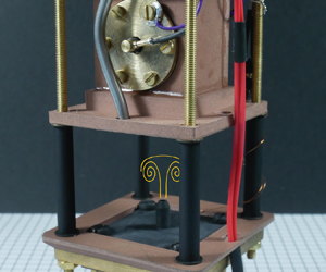
The main part of the set-up used for this study is the experimental cell sketched in figure 1(a), submerged in He II at the bottom of a pumped helium cryostat, in a volume equipped with optical ports – see Švančara (Reference Švančara2021) for a recent and detailed description of our cryogenic apparatus.

Figure 1. (a) Sketch of the experimental cell (dimensions are in millimetres). The dashed white lines indicate the open volume inside the heater box, at the bottom, and the second sound channel, at the top. Typical data as functions of time: (b) released power pulse; (c) temperature modulation inside the heater box; (d) particle trajectories visualized approximately  $15$ mm above the nozzle, in experimental conditions different from those of other panels, noted below; (e) relative amplitude of the second sound signal, at the location of the two sensors, with blue (red) indicating the upper (lower) sensor. Data in (b,c,e) were obtained by averaging
  $50$ ring realizations, with
  $T = 1.31$ K,
  $P = 0.24$ W and
  $\tau = 0.52$ s; data in (d) represent a single vortex ring, with
  $T = 1.66$ K,
  $P = 0.67$ W and
  $\tau = 0.22$ s (the mean vertical velocity of the tracked particles is removed, and the lighter colours are associated with earlier times).
The heater box, i.e. the chamber filled with He II where heat is released to generate the rings, is a custom-made, 3D-printed volume, having plastic walls and located at the bottom of our experimental cell. It is equipped with a planar resistive heater, at the bottom, and it is open at the top to the surrounding helium bath through a circular nozzle, machined from brass. The inner diameter of our nozzle is  $d = 2$ mm, and its height is
  $5d$ – the latter also includes the thickness of the brass plate covering the top part of the heater box. Each power pulse is monitored by two synchronized multimeters, to ensure that the released power pulses are neatly orthogonal, as shown in figure 1(b). Shortly after the pulse is released, we observe that the temperature inside the box temporarily increases, as displayed in figure 1(c). This is probed directly by a sub-millimetre low-temperature thermometer, made of germanium, located inside the heater box. Another thermometer is mounted at the top of the cell to ensure that the helium bath temperature remains constant.
The rings then appear above the nozzle and move vertically, similarly to the observations of our previous study (Švančara et al. Reference Švančara, Pavelka and La Mantia2020), performed with a different heater box and larger nozzle. First, the rings travel across an open volume, where they can be visualized. We employ specifically the particle tracking velocimetry technique, which is based on following the flow-induced motions of relatively small particles – see Švančara et al. (Reference Švančara2021) for another recent example. Our  $\mathrm {\mu }{\rm m}$-sized particles are made of solid deuterium; they are illuminated with a
  $1$ mm thick laser sheet crossing the symmetry axis of the set-up, and their motion is captured by a high-speed digital camera with a narrow depth of field. Since the thicknesses of the light sheet and the camera depth of field are comparable in size to the nozzle diameter, the goal of capturing the in-plane motion of our particles is achieved by removing trajectories shorter than 50 points, which might be affected significantly by out-of-plane motion.
Typical particle trajectories are plotted in figure 1(d), in the reference frame moving with the mean particle velocity in the vertical direction (in this case, the tracks are at least 100 points long, and light colours are associated with earlier times within the chosen interval). One can see clearly that particle trajectories are significantly bent near the ring core, and that the ring moves upwards along a straight line. Note, however, that, in order to get an even clearer picture, one would need more particles, especially to track the ring in time, as was demonstrated, for example, by Outrata et al. (Reference Outrata, Pavelka, Hron, La Mantia, Polanco and Krstulovic2021) in their figure 1, where the displayed ring is larger and slower than the present ones, with  $Re \approx 10^5$ – see again Švančara et al. (Reference Švančara, Pavelka and La Mantia2020). Indeed, as detailed below, flow visualization data are employed here to show that the studied flows are restricted in space and time, but unfortunately, their detailed structure, e.g. the associated small-scale vorticity distribution, is currently unknown and its investigation might be the focus of future studies.
The vortex ring then enters the second sound channel, which has a square cross-section of  $10$ mm sides. It is equipped with two second sound sensors placed
  $36$ mm apart and rotated by
  $90^{\circ }$ relative to each other. Each sensor consists of two identical transducers mounted on the opposite sides of the channel. The central element of the transducer is a gold-plated membrane that is permeable only to the superfluid component because
  $\mathrm {\mu }{\rm m}$-sized holes on this membrane do not allow the normal component to go through – see Varga et al. (Reference Varga, Jackson, Schmoranzer and Skrbek2019) for details. Each membrane is coupled capacitively to a brass electrode. The transducer emits second sound waves when we supply its electrode with a sine voltage wave, which sets the membrane (and the normal fluid component) into harmonic motion. The corresponding sound amplitude is then read by the transducer on the opposite side of the cavity in the form of voltage oscillations, induced on the corresponding electrode, using a lock-in amplifier.
In particular, a standing wave of second sound occurs in the sensor cavity when the driving signal frequency  $f$ equals the resonance frequency
  $f_k$ of the channel, given by
 \begin{equation} f_k = \frac{kc_2}{2\delta}, \end{equation}
where  $k$ is a positive integer,
  $c_2$ denotes the speed of second sound, also tabulated by Donnelly & Barenghi (Reference Donnelly and Barenghi1998), and
  $\delta = (10.3 \pm 0.3)$ mm is the effective channel width, obtained by measuring experimentally the frequencies of several resonant modes. Frequency sweeps across the resonant modes are found to be Lorentzian, indicating that the flow-probing waves do not measurably affect the flow occurring between the transducers. In quiescent He II, we measure the resonant amplitude
  $A_0$, typically of the order of
  $1$ mV, and the half-width
  $\varDelta _0$, of the order of
  $10$ Hz – the exact values vary with temperature and depend also on the sensor history. However, in order to investigate how a propagating vortex ring attenuates the second sound signal, we have to constantly excite a standing wave across the channel. In this case, the resonance condition is maintained at all times by adjusting the driving frequency via a PID loop, and the time-dependent resonance amplitude
  $A(t)$ is acquired by the lock-in amplifier at the mean sampling rate of about
  $14$ Hz. To avoid cross-talk between the sensors, we operate them independently using two distant resonance modes. Typical second sound responses to a vortex ring are displayed in figure 1(e), where we plot the relative amplitude
  $A(t)/A_0$ as a function of time – the blue (red) line corresponds to the upper (lower) sensor. The passage of the ring is detected as a sudden decrease of the signal, followed by a gradual recovery. Note also that each ring encounters remnant quantized vortices, naturally present in He II, along its path. Typically, these vortices originate from previous ring realizations, or they are pinned to solid walls, and their density falls below the resolution threshold of our second sound sensors; that is, two consecutive ring realizations are spaced in time in such a way that the acoustic amplitude of each sensor fully recovers to its original state.
We here employ (1.4) to estimate the vortex line density  $L$ from the experimentally obtained values of relative amplitude. As already noted, this relation is valid only for homogeneous and isotropic tangles, and an error of the order of
  $10\,\%$ is typically associated with it, at least in the range of experimentally accessible vortex line densities – see again Varga et al. (Reference Varga, Jackson, Schmoranzer and Skrbek2019). Specifically, for polarized vortex tangles, the experimentally accessible quantity becomes the projection
  $L_\perp$ of the vortex tangle into the direction of the second sound wave. It can be shown that
  $L_\perp \propto \langle \sin ^2\theta \rangle$, where
  $\theta$ is the angle between a small vortex line segment and the wave vector of the incident second sound wave – the brackets denote the average over all such segments of the vortex tangle. For an unpolarized tangle,
  $\langle \sin ^2\theta \rangle = 2/3$, and by definition,
  $L_\perp = L$. Instead, for an array of coplanar vortex loops, which can be used to approximate a macroscopic vortex ring,
  $\langle \sin ^2\theta \rangle = 1/2$. Relation (1.4) then overestimates the actual vortex line density by a factor
  $(2/3)/(1/2) = 4/3$ at most, and in the more realistic scenario of partial tangle polarization, we do not expect the ratio
  $L/L_\perp$ to be significantly larger than 1.
In addition, the second sound attenuation technique falls short when the amplitude  $A_0$ is measured in an environment containing a significant density of remnant quantized vortices, which are always present in any sufficiently large volume of He II, as noted above. The results obtained from (1.4) are necessarily relative to this remnant density – which is typically of the order of
  $10^6$ m
 $^{-2}$ (Varga et al. Reference Varga, Jackson, Schmoranzer and Skrbek2019) – and consequently, quantitative comparisons of results obtained in different experimental facilities are not always possible.
In this regard, it is also useful to note that the accuracy of the reported second sound measurements at present cannot be quantified because no other means to measure the vortex line density  $L$ was available during the experiments. More generally, for many years the second sound attenuation technique has been the only means to estimate experimentally the vortex line density in flows of He II (Varga et al. Reference Varga, Jackson, Schmoranzer and Skrbek2019), and only recently have other experimental tools been proposed to measure
  $L$ (Hrubcová, Švančara & La Mantia Reference Hrubcová, Švančara and La Mantia2018; Kubo & Tsuji Reference Kubo and Tsuji2019). However, these visualization-based methods work only if flow scales smaller than the mean distance between quantized vortices are accessible experimentally, and as discussed below, this is not the case for the present experiments.
In summary, in order to compare different ring realizations, obtained in the same experimental facility, we use here (1.4). This is justified mainly by the assumption that the polarization of the vortex tangles associated with our rings does not vary significantly between data sets, which might be the case, given the extremely high values of the Reynolds number achieved here (and reported below). Additionally, we make sure that  $A_0$ remains approximately constant during our experiments, i.e. we make sure that the density of remnant quantized vortices does not grow significantly during our experiments.
2.1. Reproducibility
We have already reported (Švančara et al. Reference Švančara, Pavelka and La Mantia2020) that thermal generation of vortex rings offers a high level of reproducibility. Particle trajectories originating from the visualization of multiple rings obtained under similar initial conditions provide a similar physical picture. Therefore, we can ensemble average these realizations, i.e. overlap sets of trajectories and treat the resulting data as a single ring realization.
In addition, we observe a neat overlap of the respective second sound amplitudes. Since our set-up offers the possibility of acquiring the second sound responses of a large number of vortex rings in a relatively short time, we report  $2643$ successful ring realizations probed by this technique. Our data are split into
  $53$ sets characterized by the bath temperature
  $T$, and the mean power
  $P$ and duration
  $\tau$ of the power pulse. Each data set contains between
  $39$ and
  $60$ realizations, which are ensemble averaged using
  $70$ ms wide time windows relative to the heat pulse start. We illustrate this process in figure 2 for two data sets collected at
  $1.31$ K. Colour lines denote ensemble averages of
  $50$ realizations, and pale areas represent one standard deviation intervals. We see that the signal, i.e. the relative second sound amplitude
  $A(t)/A_0$, clearly extends from the statistical error. In figure 2(a), the signal is only weakly attenuated and the corresponding standard deviation is about
  $5 \times 10^{-3}$. When the signal is considerably attenuated, as in figure 2(b), the fluctuations do not increase appreciably and the corresponding statistical error is comparable to the line thickness.

Figure 2. Relative second sound amplitude as a function of time for the upper (blue) and lower (red) sensors. Lines are ensemble averages of  $50$ realizations; pale areas indicate one standard deviation intervals. (a) Mean temperature
  $T = 1.31$ K, power
  $P = 0.10$ W, and pulse duration
  $\tau = 0.33$ s; (b)
  $T = 1.31$ K,
  $P = 0.24$ W and
  $\tau = 0.52$ s, as in figure 1(e).
It is now time to justify the choice of the suitable area  $a$, needed to estimate the normal fluid velocity, from (1.2), and the Reynolds number, from (1.3). The obvious solution is to take the nozzle area, i.e.
  $a_p = {\rm \pi}d^2/4$. The latter choice, however, results in very high values of normal fluid velocity, much higher than the values of particle velocity that one gets from ring visualization. This in essence means that there are heat leaks, i.e. the supplied heat does not exit the ring generation chamber solely through the nozzle – in the present case, it is likely that heat also leaks where the plastic heater box is joined to the brass nozzle. Consequently, the area
  $a$ should be larger than the nozzle area, and for the present experiment, we find that setting
  $a = 100$ mm
 $^2$ leads to normal fluid velocities of the same order as the particle velocities, with
  $a / a_p \approx 30$, which is a value very close to that used in our previous study (Švančara et al. Reference Švančara, Pavelka and La Mantia2020). Additionally, as discussed below, one can estimate the vortex line density
  $L$ from the Reynolds number
  $Re$, using (3.3), and
  $L$ values of the same order as those measured by the second sound sensors are found if
  $a = 100$ mm
 $^2$. In summary, the choice of
  $a$ depends on the ring generation chamber, and consequently the Reynolds number values given here can be regarded only as first-order estimates, which nevertheless allow us to perform consistent comparisons between different experimental conditions.
3. Results and discussion
Three tunable parameters, namely the helium bath temperature  $T$, the heating power
  $P$, and the power pulse duration
  $\tau$, define the initial conditions for ring generation. The precise control over these parameters results in relatively small fluctuations. We found specifically that in the range of investigated parameters, the standard deviation of
  $T$ is less than
  $1$ mK, that of
  $P$ is less than
  $1$ mW, and that of
  $\tau$ is typically around
  $10$ ms.
The rings were generated at four temperatures, equal to approximately  $1.30$,
  $1.50$,
  $1.65$ and
  $1.80$ K. These temperatures correspond to a relatively wide range of density ratios between normal and superfluid components, from
  $5$ %, at the lowest
  $T$, to approximately
  $45$ %, at the highest
  $T$. The temperature range was limited by the minimum temperature that could be achieved stably in the cryostat, and by the fact that for temperatures higher than
  $1.80$ K, we did not observe clear second sound resonances. The heating power of the pulses was between
  $0.1$ and
  $0.7$ W, and their duration ranged from
  $0.2$ to
  $1.5$ s, with
  $Q = P \tau$ not exceeding
  $0.75$ J, because the characteristic shape of the second sound signal, apparent from figure 2, became deformed for larger
  $Q$ values in the present set-up. (This deformation might originate from collisions of the generated flow structures with the walls of the second sound channel.)
Figure 3 displays how the data sets sample the parameter space given by the Reynolds number  $Re$, (1.3), and the dissipated heat
  $Q$. As already noted, we achieved
  $Re$ values between
  $2 \times 10^4$ and
  $4 \times 10^6$ – the kinematic viscosity of He II is of the order of
  $10^{-8}\,{\rm m}^2\,{\rm s}^{-1}$ in the current temperature range. Therefore, we consider all rings to be turbulent, because the onset of turbulence is expected for
  $Re \gtrsim 10^4$ (Glezer Reference Glezer1988).


Additionally, as detailed below, we observe flow structures having sizes along the set-up (vertical) axis significantly larger than those in the perpendicular (horizontal) direction. These long structures can be associated with prominent wakes that originate from the excess fluid discharge, and can be observed past vortex rings, as discussed e.g. by Gharib, Rambod & Shariff (Reference Gharib, Rambod and Shariff1998). In this regard, a relevant parameter is the formation number  $F$, defined as the ratio between the piston stroke and the nozzle diameter (Gharib et al. Reference Gharib, Rambod and Shariff1998). The vortex ring pinch-off is usually observed for
  $F \approx 4$, as reported e.g. by Krueger, Dabiri & Gharib (Reference Krueger, Dabiri and Gharib2006) and Krieg & Mosheni (Reference Krieg and Mosheni2021), while, for higher stroke-to-diameter ratios, the ring is followed by a trailing jet, which we identify here as the wake. We calculate the formation number as
  $F = x/d$, where the stroke length
  $x$ is defined by (1.1). Following § 2.1, we take
  $a = 100$ mm
 $^2$ for the calculation of
  $x$, and we find that our rings sample a relatively wide range of formation numbers, from approximately
  $6$ to
  $148$, with median value
  $25$. This indicates clearly that the studied rings should be followed by prominent wakes, and as shown below, this view is supported strongly by the experimental data.
Note in passing that in our previous study (Švančara et al. Reference Švančara, Pavelka and La Mantia2020), we achieved relatively smaller  $Re$ values, between approximately
  $10^4$ and
  $10^5$, for power pulses of comparable power and duration, with
  $Q$ up to approximately
  $2.75$ J, using a larger nozzle,
  $5$ mm in diameter. Additionally, Švančara et al. (Reference Švančara, Pavelka and La Mantia2020) observed the behaviour of macroscopic vortex rings in the nozzle proximity, at distances between
  $1$ and
  $6$ nozzle diameters, while in the following we report results obtained at larger distances, up to
  $40$ nozzle diameters.
3.1. Spatial and temporal confinement
The confinement of vortex rings in space and time was verified by flow visualization. We focus specifically here on three representative data sets, named R1, R2 and R3. They were collected at  $1.80$ K, with
  $P = 0.48$ W and three different
  $\tau$ values, equal to
  $0.33$,
  $0.52$ and
  $1.02$ s, for R1, R2 and R3, respectively. Therefore, these sets are characterized by different values of dissipated heat
  $Q$, as shown in figure 3, where we highlight R1, R2 and R3 using coloured circles.
These rings are associated with formation numbers  $F$ equal to
  $5.6$,
  $9.0$ and
  $17.7$ for R1, R2 and R3, respectively. In the following, for the sake of comparison, we set the non-dimensional time
  $\hat {t} \equiv v_n t/d$, so that for
  $t = \tau$,
  $\hat {t} = F$ (Limbourg & Nedić Reference Limbourg and Nedić2021). We also use the non-dimensional velocity
  $\hat {v} \equiv v/v_0$, where
  $v_0 = 2.3\,{\rm mm}\,{\rm s}^{-1}$ is the absolute value of the settling velocity of deuterium particles. As in previous studies, e.g. Švančara et al. (Reference Švančara2021), for the estimate of
  $v_0$ we employed the Stokes formula, assuming spherical particles with radius equal to
  $5\,\mathrm {\mu }$m (the density of solid deuterium is set to
  $200\,{\rm kg}\,{\rm m}^{-3}$, and the fluid temperature is set to
  $1.80$ K).
Particle motions were tracked within a planar field of view (FOV),  $6.2d$ wide and
  $3.9d$ high, during a
  $\hat {t} \approx 80$ long time window (the reference length is here the nozzle diameter
  $d$). The FOV bottom edge was
  $7.7d$ above the nozzle top. Qualitatively, the acquired trajectories match those displayed in figure 1(d), although, as already mentioned, the present visualization data do not allow us to track the rings as in our previous study (Švančara et al. Reference Švančara, Pavelka and La Mantia2020), mainly because here the rings are smaller and faster. Instead, to assess the flow quantitatively, we first calculated the particle velocity by convoluting each particle trajectory with a suitably defined kernel – the method is discussed in detail by Švančara (Reference Švančara2021). For each data set, several realizations were collected and ensemble averaged, so that at least one million particle positions (velocities), organized in trajectories that contain at least
  $50$ points each, are available for the analysis, which consists in studying the resulting position–velocity pairs.
The coloured lines in figure 4 display the mean vertical velocity, i.e. the mean particle velocity in the (vertical) direction of ring propagation, conditioned by the horizontal position. We identify a region in the middle of the camera FOV characterized by a large positive velocity, indicating that in that region, the particles move upwards on average. Note in passing that since the rings are turbulent, one could say that most of the detected particles are advected by the wake rather than by the ring itself.

Figure 4. Mean vertical velocity conditioned by the horizontal particle position in non-dimensional units. Coloured lines indicate data sets R1–R3; grey lines denote velocity profiles restricted to the bottom, middle and top thirds of the camera FOV, from R3; black solid lines denote Gaussian fits of the velocity profiles (see § 3.1); the red dashed line indicates the estimated settling velocity of solid deuterium particles in He II, corresponding to  $\hat {v} = -1$. In the employed non-dimensional units, the nozzle diameter is equal to
  $1$.
$1$.
The observed peaks of positive velocity can be described accurately with vertically shifted Gaussian curves – the best fits are marked by solid black lines. The offsets yield  $\hat {v} \approx -1$, which reflects clearly the settling of our particles (see the red dashed line in figure 4). More importantly, the centres and widths of the Gaussian peaks share similar values. This means that the vortex rings propagate along the same vertical trajectory, and that their size does not significantly vary among data sets.
In addition, we checked that for R3, a similar velocity profile is obtained at the bottom, middle and top thirds of the FOV – these profiles are displayed in figure 4 as grey lines that overlap closely with the original violet curve. It therefore seems that the flow structure does not grow appreciably in the radial direction, and most likely does not grow beyond the size of the square second sound channel, equal to  $5d$.
$5d$.
Specifically, we find the standard deviation of each peak to be  $\sigma \approx 0.7 d$, which can be taken as the estimate of the ring radius at a distance from the nozzle equal to approximately
  $10d$. It then follows that at distance
  $40d$, the ring radius should be less than
  $1.5 d$, if one assumes that for distances larger than
  $15 d$, the growth rate of turbulent rings is
  $0.01$, as reported by Maxworthy (Reference Maxworthy1974) – note that on the basis of figure 4, we set to
  $0.1$ the growth rate at smaller distances. Consequently, this estimate allows us to neglect possible effects of the channel walls on the generated flow, at least for the present set-up.
We take again R3 as a representative example, and we plot in figure 5 how the mean particle velocity evolves in time if we restrict our FOV to a finite interval in the horizontal direction. The selected intervals, specified in the legend, are centred at the peak position (about  $3.1d$), and their widths correspond to
  $\sigma$,
  $2\sigma$ and
  $4\sigma$ – the light-brown curves (labelled ‘Outside’) represent the exclusion of the latter interval from the full FOV width.

Figure 5. Time dependence of the mean particle velocity when the camera FOV is confined in the horizontal direction. Data from R3 – see the legend for the considered intervals. ‘Outside’ indicates the exclusion of the third interval from the full FOV width. Particle velocity and time are normalized according to the main text. (a) Horizontal velocity component; (b) vertical velocity component.
The mean horizontal velocity, plotted in figure 5(a) as a function of time, remains unaffected by the propagating ring. However, a distinct velocity peak develops for the vertical component, displayed in figure 5(b), shortly after the heat pulse is released at  $\hat {t} = 0$. The particle velocity then decreases until the mean particle velocity becomes nearly zero, which confirms that the flow is indeed confined in time. Additionally, the response to the heat pulse of the particles outside the considered intervals is negligible. Hence we can conclude that the flow consisting of a vortex ring and its wake extends no more than
  $4\sigma = 2.8d$ in the horizontal direction, which we can take as an upper limit for the vortex ring size in that direction, at least for the considered data sets.
The differences among the studied data sets are highlighted in figure 6. For all three cases, we restrict the FOV to the interval  $3.1d + [-\sigma,\sigma ]$ and observe only the vertical velocity component. The figure clearly indicates that the peak velocities are different and grow with increasing
  $\tau$. In other words, power pulses of different durations produce qualitatively different vortex rings, consistently with the definition of the Reynolds number, (1.3). Nevertheless, we now show that the propagation of thermally generated vortex rings can also be defined by another parameter, which is the temporary temperature increase inside the heater box.

Figure 6. Mean vertical velocity as a function of time, when the FOV is restricted to the horizontal interval  $3.1d + [-\sigma,\sigma ]$, i.e.
  $[2.4d,3.8d]$.
3.2. Temperature increase
The existence of a brief temperature increase inside the heater box has been reported already in figure 1(c) for an exemplary case. Following our reproducibility remarks in § 2.1, we ensemble averaged our temperature data sets and calculated the maximum difference  $\Delta T$ between the bath and box temperatures. A first-order theoretical estimate of
  $\Delta T$ can be based on the assumption that the supplied heat
  $Q$ adiabatically warms up the content of the heater box. We can then write
 \begin{equation} \Delta T \approx \frac{Q}{\rho V_b c}, \end{equation}
where  $V_b = 11\,{\rm cm}^3$ denotes the inner volume of the heater box, and
  $c$ is the specific heat of He II, also tabulated by Donnelly & Barenghi (Reference Donnelly and Barenghi1998) as a function of temperature.
Despite the model simplicity, we observe a linear relation between  $\Delta T$ and
  $Q/(\rho c)$ in the experimental data, displayed as blue points in figure 7(a). The linear fit, i.e. the black line in the same figure, yields a practically zero intercept and a non-zero slope that gives an estimate of the effective box volume,
  $V_{eff} \approx 3V_b$. The difference between
  $V_b$ and
  $V_{eff}$ is due to the heat leaks from the heater box, mentioned above, which are expected to take place through its walls and through the nozzle, as the latter mechanism is actually responsible for the generation of vortex rings. Note also that
  $\Delta T$ is a function of all tunable parameters, because
  $Q$ depends directly on
  $P$ and
  $\tau$, and
  $c$ displays a strong temperature dependence – it grows with increasing
  $T$ in the investigated range, while
  $\rho$ does not vary appreciably with
  $T$, as already noted.

Figure 7. (a) Maximum difference  $\Delta T$ between the helium bath and the heater box temperatures as a function of
  $Q/(\rho c)$. Blue points indicate experimental data; black line indicates the linear fit. (b) Duration of the increased temperature period
  $t_{\Delta T}$ inside the heater box as a function of
  $Q/(\rho c)$; see § 3.2 for details.
Beside the finite temperature increase, figure 1(c) also shows that the duration of this temperature increase, which can be associated with the ejection of the normal component from the heater box, is finite and larger than the duration  $\tau$ of the corresponding heat pulse; see figure 1(b). We estimate the former time period,
  $t_{\Delta T}$, as the interval during which the temperature difference between the heater box and the helium bath is at least
  $0.1 \Delta T$. We find that, as expected,
  $t_{\Delta T}$ increases with
  $\tau$, and in figure 7(b), we plot
  $t_{\Delta T}$ as a function of
  $Q/(\rho c)$. In contrast to figure 7(a), this quantity displays a less clear scaling with
  $Q/(\rho c)$, likely because the temperature sampling frequency was significantly smaller than that of the power, but one cannot deny that the two quantities are positively correlated, i.e.
  $t_{\Delta T}$ also increases with
  $Q/(\rho c)$. Moreover, the maximum duration of this time period is less than
  $5$ s, which is smaller than the typical duration of our second sound response, shown in figure 1(e) and discussed below.
Additionally, it is worth mentioning here that for thermal counterflow jets, Murakami, Yamakazi & Nakai (Reference Murakami, Yamakazi and Nakai1989) reported an analogous linear relation between the heater box temperature increase and the applied heat flux  $q = P/a$, at
  $q$ values smaller than approximately
  $5\,{\rm kW}\,{\rm m}^{-2}$, while at larger values of heat flux, it was found that
  $\Delta T \propto q^3$ – these scalings can be related to the above-mentioned dependence between the mutual friction force and the relative fluid velocity, discussed, for example, by Ricci & Vicentini-Missoni (Reference Ricci and Vicentini-Missoni1967) and Liepmann & Laguna (Reference Liepmann and Laguna1984). Nevertheless, considering that for the present data sets, the maximum
  $q$ value is lower than
  $7\,{\rm kW}\,{\rm m}^{-2}$, with
  $a = 100$ mm
 $^2$, we may conclude that the results presented in figure 7(a) are consistent with our current understanding of thermally generated flows of He II, outlined in § 1; that is, no cubic scaling is apparent from our data because our maximum value of heat flux is very close to the critical value identified by Murakami et al. (Reference Murakami, Yamakazi and Nakai1989) – note also that the corresponding median value is lower than
  $5\,{\rm kW}\,{\rm m}^{-2}$. Finally, we would like to emphasize that the observed linear relation between
  $\Delta T$ and
  $q$ does not imply that the observed flow structures are not turbulent. The opposite is true, because, as already noted, the Reynolds numbers associated with them are very large, and as shown below, their generation is linked to the ejection of dense vortex tangles, detected by our second sound sensors.
3.3. Vortex line density profiles
A vortex line density (VLD) profile is defined here as the time dependence of VLD, also named  $L$, calculated from the acquired second sound amplitude using (1.4). Typical
  $L$ profiles are plotted in figures 8(a,b) for the upper and lower sensors, respectively – the displayed profiles result from identical power pulses (
 $P = 0.48$ W,
  $\tau = 0.52$ s), and their differences are due solely to the different temperatures of the helium bath (see the legend). Each profile displays negligible VLD values before the power pulse, which are followed by a distinct peak that develops some time after. Note in passing that the small
  $L$ jump in figure 8(a) is likely due to cross-talk between the wires inside the cryostat. The dominant feature of each profile is its long-lasting tail that gradually returns the sensor to its original state. The characteristic shape of these profiles matches the idea outlined above that these signals may indeed represent turbulent vortex rings; that is, the peak indicates a dense and compact bundle of quantized vortices, while the decaying part can be associated with the trailing jet. Note also that a similar profile shape is observed for all data sets and for both sensors. Additionally, the peak measured by the upper sensor is systematically less pronounced than the other, and it is observed with a small delay – the sensors must therefore respond to the same object that travels along the second sound channel.

Figure 8. Ensemble-averaged vortex line density (VLD) profiles obtained by releasing a power pulse with  $P = 0.48$ W and
  $\tau = 0.52$ s: (a) data from the upper sensor,
  $81$ mm above the nozzle; (b) data from the lower sensor,
  $45$ mm above the nozzle. The coloured lines indicate the temperature of the helium bath.
The VLD profiles that correspond to the same vortex ring (data set) are plotted in figure 9, for the upper (blue) and lower (red) second sound sensors. The finite time lag between the peaks, now clearly visible, is used in § 3.5 to estimate the ring propagation velocity. Interestingly, we note that the late-time parts of these profiles overlap closely and follow an exponential decay (see the inset). This result, taking place for all available data sets, can be associated with the ring trailing jet, as already mentioned, but it might also be explained by considering that quantized vortex loops somehow could be released from the dense vortex tangle centred near the vortex ring. Additionally, the presence of this flow structure is consistent with the numerical simulations reported by Kivotides (Reference Kivotides2015), showing that quantized vortex loops tend to concentrate in the proximity of a normal fluid vortex ring as it moves through a sample of He II with a few remnant vortices.

Figure 9. Detailed view of typical VLD profiles obtained by the upper (blue) and lower (red) sensors. Here,  $T = 1.31$ K,
  $P = 0.48$ W and
  $\tau = 0.52$ s. Inset: late-time parts of the profiles plotted in log-linear scale.
In summary, the VLD profiles obtained across several temperatures and power pulses display a typical shape that reflects clearly the physical nature of the studied flow. A dense, coherent bundle of quantized vortices is observed to propagate along the channel, followed by a turbulent wake. Additionally, despite its notable decrease in magnitude, the flow structure remains coherent along a path at least  $40$ nozzle diameters long, which is the maximum distance that we can probe currently.
3.4. Circulation of the vortex bundle
In order for the quantized vortex tangle to mimic a macroscopic vortex ring, it must be at least partially polarized, i.e. it must display a non-zero circulation  $\varGamma$. For an array of coplanar vortex loops, i.e. for a fully polarized tangle, such a circulation can be written as
 \begin{equation} \varGamma = \kappa n A_c, \end{equation}
where  $\kappa$ indicates the quantum of circulation,
  $n$ denotes the number of quantized vortices per unit area, and
  $A_c$ is a relevant cross-sectional area of the considered large-scale vortex ring (we assume here that quantized vortices are perpendicular to this area). It then follows that for a fully polarized tangle, the vortex ring core must contain a total vortex length
  $\mathcal {L} = 2{\rm \pi} R n A_c$, where
  $R$ is the ring radius, which in our case is equal to around
  $2$ mm, at a distance from the nozzle of approximately
  $10d$, as discussed in § 3.1 – note, once more, that
  $R$ is parallel to
  $A_c$. Additionally, these vortices were detected by our sensors within a detection volume
  $V_d \approx 500$ mm
 $^3$ – our channel is
  $10$ mm wide, and the diameter of a second sound transducer is
  $8$ mm. Therefore, the measured VLD can be written as
 \begin{equation} L = \frac{\mathcal{L}}{V_d} = \frac{2 {\rm \pi}R n A_c}{V_d} = \frac{2 {\rm \pi}}{\kappa V_d}\,R \varGamma = \frac{2 {\rm \pi}\nu}{\kappa V_d}\,R\,Re, \end{equation}
where we used (3.2) and the slug flow model relation  $Re = \varGamma / \nu$, reported in § 1.
From (3.3) one can then calculate that for  $Re \approx 3.3 \times 10^{4}$ and
  $T = 1.80$ K, corresponding to R2 in § 3.1, a fully polarized tangle yields
  $L \approx 7.4 \times 10^{7}$ m
 $^{-2}$, which is a value rather close to that measured by the lower sensor, shown in figure 8(b) – for this estimate, we set
  $R = 2$ mm in (3.3). Consequently, closer agreement with the experimental data can be obtained for larger values of the vortex ring radius, which are actually expected to occur, as discussed in § 3.1 (e.g.
  $L \approx 1.1 \times 10^{8}$ m
 $^{-2}$ for
  $R = 3$ mm), or considering that for turbulent rings, the length of a quantized vortex within the ring might be larger than the ring circumference, because waves may occur along the vortex, as discussed, for example, by Švančara & La Mantia (Reference Švančara and La Mantia2019). Similarly, a two times larger value of
  $Re$ would result, for
  $R = 2$ mm, in a VLD equal to approximately
  $1.5 \times 10^{8}$ m
 $^{-2}$, which is a value much closer to the experimental finding reported in figure 8(b) – such a
  $Re$ value could be obtained from (1.3) by setting in (1.2) the heater area
  $a$ to approximately
  $70$ mm
 $^2$, at the given values of
  $P$ and
  $\tau$.
Nevertheless, as already noted, the Reynolds numbers reported here can be considered solely as first-order estimates, and it is actually remarkable that one can get from (3.3) values of VLD that are of the same order of magnitude of those measured experimentally, especially considering the many assumptions made in the derivation of (3.3). In other words, (3.3) can be seen as an expression identifying the main parameters contributing to  $L$, rather than a quantitative measure of the VLD associated with our macroscopic vortex rings.
However, it is also useful to estimate the number  $n A_c$ of vortex loops embedded in one of our rings, using (3.3) with
  $\varGamma = \nu \,Re$. Specifically, from the
  $Re$ values plotted in figure 3, we obtain that the superfluid component should contain at least
  $10^3$ quantized vortices. Additionally, considering that the mean distance
  $\ell$ between quantized vortices can be estimated as
  $1/\sqrt {L}$, we find that for the data set just discussed,
  $\ell \approx 120\,\mathrm {\mu }$m, which is a value much smaller than the resolution of our experiment. Therefore, one can say that we currently probe the vortex tangle in a regime where individual quantized vortices cannot be resolved.
Now, if we assume that the tangle polarization does not change appreciably among our data sets, which might be the case, given the extremely high  $Re$ values, then we can estimate qualitatively the circulation of the vortex tangle by using the maximum
  $L_m$ of each VLD profile. This quantity is plotted in figure 10 as a function of the dissipated heat
  $Q$. We observe that the
  $L_m$ values detected by both sensors – see figures 10(a,b) for the upper and lower sensors, respectively – scale (almost) linearly with
  $Q$ – one can indeed note that this linear dependence is less robust for the lower sensor, especially at the smaller temperatures, which might be an effect of the nozzle proximity. Additionally, the maximum VLD values display a temperature dependence similar to the VLD profiles plotted in figure 8.

Figure 10. Maximum profile density  $L_m$ as a function of the dissipated heat
  $Q$, for the (a) upper and (b) lower second sound sensors.
Strikingly, the helium bath temperature dependence is removed when  $Q$ is replaced by
  $\Delta T$, and the data collapse onto two lines (one line per sensor), as we show in figure 11(a). We checked this further by comparing the present result with the data sets labelled G1. These sets were obtained with the first generation of our experimental cell, at temperatures
  $1.51$ and
  $1.66$ K – see Švančara (Reference Švančara2021) for details and preliminary results. Note that this cell featured only one second sound sensor, located
  $68$ mm away from the nozzle, and that the heater box lacked temperature monitoring. In order to compute
  $\Delta T$ for the G1 data, we simply employed the linear fit from figure 7(a), using the known bath temperature and power pulse parameters.

Figure 11. (a) Maximum VLD as a function of  $\Delta T$. Symbols as in figure 10, plus grey symbols labelled G1: data obtained by the first generation of the experimental cell (see § 3.4). (b) Slopes of the collapsed dependencies from (a) as a function of the distance between the nozzle top and the position of the corresponding second sound sensor.
Therefore, it is apparent from figure 11(a) that the maximum value  $L_m$ of the VLD
  $L$ is proportional to
  $\Delta T$, at least in the range of investigated parameters. Additionally, considering (3.3), one can write that
  $\varGamma \propto L / R \propto \Delta T / R$, which means, on the basis of (3.1), where
  $\Delta T \propto Q = P \tau$, that
  $\varGamma \propto P \tau / R$. On the other hand, from (1.3), we see that
  $\varGamma \propto P^2 \tau$, because, from the slug flow model,
  $\varGamma \propto Re$. It then follows that the applied power
  $P$ should be inversely proportional to the ring radius
  $R$, and that on the basis of (1.2), the same applies to the normal fluid velocity
  $v_n$. Consequently, the outcome is consistent with the classical theory on the propagation of turbulent vortex rings in Newtonian fluids, discussed by Maxworthy (Reference Maxworthy1974), if we assume that, at a given temperature, the normal fluid velocity is proportional to (some power of) the vortex ring velocity
  $U$, and that
  $R$ is proportional to the distance
  $z$ travelled by the ring, because
  $U$ is expected to be proportional to
  $z^{-(3+C)}$, where
  $C$ is a (drag) coefficient of order 1 (Maxworthy Reference Maxworthy1974). In short, it appears that the propagation of macroscopic vortex rings in He II can be described by theories developed for classical rings, at least to a first approximation.
The latter statement is reinforced if we look more closely at the decay of the vortex tangle. Indeed, according to Maxworthy (Reference Maxworthy1974), the ring circulation  $\varGamma$ is expected to scale as the ring velocity times
  $R$, and from (3.3), we see that
  $L \propto R \varGamma$. Then, considering that
  $R$ scales as the distance
  $z$ travelled by the ring, and that for classical rings,
  $\varGamma$ is expected to scale as
  $z^{-(2+C)}$, it follows that
  $L$ should be inversely proportional to some power of
  $z$ larger than 1 (Maxworthy Reference Maxworthy1974). Actually, the curves broadly collapse if
  $L_m (z / d)^2$ is plotted as a function of
  $\Delta T$, where
  $z / d$ denotes the dimensionless distance between the nozzle and the sensor. Once more, an outcome based on a classical theory is consistent with the results reported in figure 11(a), which were obtained in superfluid
  $^4$He – see also figure 11(b).
Specifically, it is apparent that the slope of each linear dependence in figure 11(a) is a function of only the distance between the nozzle and the second sound sensor. The VLD embedded in a ring hence decreases by the same factor, if the ring travels the same distance; for example, we observe this density to drop by approximately  $3$ times between the second sound sensors in our experimental cell. To elaborate on this, we take the slopes of the linear fits of the collapsed dependencies and plot them in figure 11(b) as a function of the distance from the nozzle. The linear extrapolation of the first and last point yields that zero slope, corresponding to vanishing VLD, occurs approximately
  $50$ nozzle diameters away from the nozzle. This value can then be understood as the maximum distance where the tangle should remain coherent. Although we did not consider other contributing factors, e.g. that the rings do slow down in time (Švančara et al. Reference Švančara, Pavelka and La Mantia2020), our experimental data confirm neatly that turbulent vortex rings propagating in He II are indeed long-lived structures that may travel a large distance relative to their size, similarly to their classical counterparts.
3.5. Ring velocity
The arrival time of a VLD peak, i.e. the time at which the VLD is equal to  $L_m$, combined with the known distance between the nozzle and a second sound sensor, provides a simple estimate of the mean ring velocity. However, such an estimate does not consider the mechanism of ring formation, which was not accessed in the present experiment. Indeed, it is expected that vortex rings actually form some distance from the nozzle and some time after the injection of momentum, as discussed, for example, by Glezer & Coles (Reference Glezer and Coles1990).
Partially motivated by this obstacle, we devised our experimental cell with two sensors, which allows us to estimate the ring propagation velocity  $w$ between these sensors as
 \begin{equation} w = \frac{D}{t_{mu} - t_{ml}},\end{equation}
where  $D = 36$ mm indicates the sensor separation, and
  $t_{mu}$ (
 $t_{ml}$) denotes the arrival time for the upper (lower) sensor. The time lag
  $(t_{mu} - t_{ml})$ is insensitive to the ring formation process, therefore (3.4) provides an estimate of the (mean) ring velocity that is more reliable than that based on just one second sound sensor.
Figure 12 displays  $w$ as a function of
  $\Delta T$. First, one may note that the range of probed ring velocities is rather wide, because the slowest rings propagate with
  $w \approx 2\,{\rm mm}\,{\rm s}^{-1}$, while the velocity of the fastest ones is approximately
  $15$ times larger. Second, we find again that all data sets collapse onto a single curve, which supports the relevance of
  $\Delta T$ as a control parameter. A single-component power law roughly matches this nonlinear dependence (see the black solid line in figure 12), but unfortunately we currently have no quantitative explanation for it (note also that for
  $\Delta T \gtrsim 0.1$ K, the reported scaling relation appears less suitable).

Figure 12. Mean ring velocity  $w$ as a function of
  $\Delta T$. Black line indicates a power-law fit with exponent
  $0.75 \pm 0.03$.
Additionally, it is important to remark that, as already noted, the gradual loss of kinetic energy results in the ring velocity decreasing. Following the similarity theory mentioned in § 3.4 (Maxworthy Reference Maxworthy1974), the propagation velocity  $U$ of a turbulent vortex ring is expected to depend on the travelled distance
  $z$ as
 \begin{equation} U = U_0 \left(\alpha\,\frac{z}{r_0} + 1 \right)^{-(3 + C)}, \end{equation}
where  $U_0$ is the initial ring velocity, and
  $\alpha \approx 0.01$ denotes the ring growth rate, also reported by Glezer & Coles (Reference Glezer and Coles1990) and Gan & Nickels (Reference Gan and Nickels2010); additionally,
  $r_0$ indicates the initial ring radius, and
  $C$ is a drag coefficient related to the entrainment of the surrounding fluid, already introduced in § 3.4. Note in passing that the present data do not allow us to verify (3.5) directly – e.g. to determine relevant values of
  $\alpha$ and
  $C$ – but in our previous work (Švančara et al. Reference Švančara, Pavelka and La Mantia2020), we showed that scaling relations related to (3.5) hold for the macroscopic vortex rings studied there, which are larger and slower than the present ones.
Nevertheless, if we assume that in the range of investigated parameters,  $\alpha$,
  $r_0$ and
  $C$ are constant, then the velocity measured at a fixed distance from the nozzle is proportional solely to the initial velocity
  $U_0$. Our data sets hence indicate that it is the initial ring velocity that also depends systematically on
  $\Delta T$. This outcome is in agreement with the visualization study summarized in § 3.1. We observed specifically that at a given power, the mean particle velocity tends to increase upon increasing the pulse duration, which is consistent with the fact that
  $\Delta T \propto Q \propto \tau$, discussed in § 3.2.
3.6. Vortex line length
The typical shape of the acquired VLD profiles suggests that each power pulse produces quantized vortices with a finite collective length. As second sound attenuation was measured in a channel with cross-section  $A_{ch} \approx 100$ mm
 $^2$, we can simply calculate the total line length
  $\mathcal {L}$ as
 \begin{equation} \mathcal{L} = A_{ch} \int_{-\infty}^\infty L(z) \,\mathrm{d}z, \end{equation}
where we integrate the VLD along the channel axis  $z$. Within this notation, we assume that the nozzle is located at
  $z = 0$, and therefore
  $L = 0$ for
  $z \leq 0$.
However, the experimentally accessible quantity is the area below each VLD profile, i.e. the VLD integrated in time,  $L_I$. The integration is performed specifically in a finite time interval, limited by
  $t_{min} = -5$ s and
  $t_{max} \geq 40$ s – these intervals were chosen for each data set individually, to make sure that they are long enough to accommodate the entire second sound signal. We can hence write that
 \begin{equation} L_I = \int_{t_{min}}^{t_{max}} L(t) \,\mathrm{d}t \approx \int_{-\infty}^\infty L(t)\, \mathrm{d}t. \end{equation}
 The relation between the integrals in (3.6) and (3.7) is not straightforward. First, the ring propagation velocity is not constant in time, as already noted, and therefore the spatial and temporal coordinates are not linked by a simple Galilean transformation. Instead, the relation  $z(t)$ is nonlinear and can be given, for example, by (3.5). Moreover, the employed sensors have a finite size, and the measured density
  $L(t)$ is not equal to
  $L[z(t)]$. Instead, the measured signal is spatially averaged within the sensitive area of the sensor, a circle with
  $d_s = 8$ mm diameter. For the simplest model of a uniform sensitivity, we can write
 \begin{equation} L(t) = \frac{1}{d_s} \int_{{-}d_s/2}^{d_s/2} L\left[ \xi + z(t)\right] \,\mathrm{d}\xi = \left(L \ast S\right)\left[z(t)\right], \end{equation}
where  $\ast$ denotes the convolution of
  $L$ with the sensor resolution function
  $S$, which is modelled as an orthogonal step function with the functional value equal to
  $1/d_s$ between
  $-d_s/2$ and
  $d_s/2$, and zero otherwise. Since the integral of
  $L$ is proportional to the vortex line length and the integral of
  $S$ is one by definition, it follows that
 \begin{equation} \int_{-\infty}^\infty L(t) \,\mathrm{d}t = \left(\int_{-\infty}^\infty S(\xi) \,\mathrm{d}\xi\right)\times \left(\int_{-\infty}^\infty L\left[z(t)\right] \,\mathrm{d}t\right) = \int_{-\infty}^\infty L\left[z(t)\right] \,\mathrm{d}t.\end{equation}
 Now, in order to link the equations above, we must simplify the nonlinear transformation between  $z$ and
  $t$. For the sake of argument, we assume that vortex rings propagate with a constant velocity, equal to the experimentally accessible value
  $w$. In other words, we estimate the right-hand side of (3.9) as
 \begin{equation} \int_{-\infty}^\infty L\left[z(t)\right] \,\mathrm{d}t \approx \frac{1}{w} \int_{-\infty}^\infty L(z) \,\mathrm{d}z,\end{equation}
where the factor  $(1/w)$ originates from the transformation Jacobian, i.e. it holds that
  $\mathrm {d}t = \mathrm {d}z/w$. Finally, using (3.6), (3.7), (3.9) and (3.10), we can estimate the vortex line length as
 \begin{equation} \mathcal{L} \approx A_{ch} w \int_{-\infty}^\infty L(t) \,\mathrm{d}t = A_{ch} w L_I.\end{equation}
 Relevant estimates of the vortex line length are plotted as a function of  $\Delta T$ in figure 13. Despite several simplifications introduced above, the experimental data display a power-law scaling with
  $\Delta T$, with an exponent close to
  $3/2$, which is marked by a solid black line. The scaling holds for both the upper sensor (empty symbols) and the lower sensor (filled symbols) – but it seems less adequate for
  $\Delta T \lesssim 0.02$ K. Additionally, systematically larger values of
  $\mathcal {L}$ are acquired by the lower sensor, in comparison with the upper one, clearly pointing out that the vortex tangle, localized either in the ring or in the wake, is subjected to dissipation.


In order to account qualitatively for the scaling presented in figure 13, we first note that a similar exponent was reported by Varga, Babuin & Skrbek (Reference Varga, Babuin and Skrbek2015) in turbulent coflow of superfluid  $^4$He, namely for steady channel flow past a grid. Specifically, it was found that in the range of probed conditions, the VLD is approximately proportional to
  $u^{3/2}$, where
  $u$ denotes the mean flow velocity in the channel used by Varga et al. (Reference Varga, Babuin and Skrbek2015). Additionally, the authors explained this outcome qualitatively on the basis of classical arguments, postulating the Newtonian-like behaviour of mechanically driven flows of He II at flow scales larger than the mean distance between quantized vortices. Similarly, Laguna (Reference Laguna1975) reported that for thermal counterflow jets, the second sound attenuation scales as
  $q^{3/2}$, where
  $q = P / a$ indicates the applied heat flux. The result, which is consistent with the scaling found by Varga et al. (Reference Varga, Babuin and Skrbek2015) if one considers (1.2) and (1.4), was explained later by Liepmann & Laguna (Reference Liepmann and Laguna1984) without taking into account the peculiar nature of helium II, i.e. using classical geometric acoustics to model the attenuation of second sound waves through the turbulent jet. In short, the scaling
  $L \propto u^{3/2}$ indicates that the steady flows studied by Liepmann & Laguna (Reference Liepmann and Laguna1984) and Varga et al. (Reference Varga, Babuin and Skrbek2015) behave as if they were those of a Newtonian fluid, at least in the range of investigated parameters.
On the other hand, from figure 11(a), it is apparent that  $L$ should scale as
  $\Delta T$, and on the basis of figure 12, one can say that the estimated ring velocity
  $w$ is proportional to some power of
  $\Delta T$ smaller than 1. It then follows that for the turbulent vortex rings investigated here, the VLD is apparently proportional to some power of the ring velocity larger than 1, which is also evident from figure 13 if one considers that
  $\mathcal {L} \propto L$ in a given volume. In conclusion, the present experimental data do not allow us to say that the scaling observed in figure 13 is the same associated to coflow by Liepmann & Laguna (Reference Liepmann and Laguna1984) and Varga et al. (Reference Varga, Babuin and Skrbek2015), mainly because it is not straightforward to define a characteristic (mean) velocity in the case of unsteady flows, such as those associated with vortex rings.
At the same time, we cannot entirely rule out such a possibility, considering especially that at larger values of heat flux  $q$, one expects a nonlinear relation between
  $\Delta T$ and
  $q$, as discussed in § 3.2, and that for steady thermal counterflow in channels,
  $L$ was found to be proportional to the square of the counterflow velocity (Varga et al. Reference Varga, Babuin and Skrbek2015). Note also that at present we cannot measure the relative fluid velocity near the nozzle, where counterflow features should be observed also for vortex rings and counterflow jets, and consequently we cannot link this relative velocity to some characteristic velocity of our rings, in view of relevant comparisons.
4. Conclusions
We have studied systematically the propagation of turbulent vortex rings in superfluid  $^4$He, at extremely high values of the Reynolds number, up to
  $4 \times 10^6$. The thermal generation mechanism, consisting of releasing an orthogonal power pulse into an enclosed volume terminated by a circular nozzle, was found to create well-defined and highly reproducible flow structures, consisting of large-scale vortex rings, in both components of He II, followed by their trailing jets. These vortical structures are confined in space and time, i.e. the observed vortex rings are characterized by a finite size, comparable to the nozzle diameter, and they propagate vertically along the nozzle axis, up to distances of at least
  $40$ nozzle diameters. In other words, we found that the tangles of quantized vortices embedded in our rings remain coherent for distances much larger than their sizes. Moreover, quantized vortices are present in the ring wakes and we also observed how their line density decreases in time, at given locations, with features independent of liquid temperature and power pulse parameters.
The vortex ring circulation, which can be related to the vortex line density via (3.3), and its characteristic velocity were found to depend neatly on  $\Delta T$, which is the experimentally accessible temperature difference between the helium bath and the heater box, occurring briefly after the ring generating power pulse is released into the He II. Specifically, we observed that vortex rings characterized by the same
  $\Delta T$ display similar behaviour, without further dependence on temperature or other power pulse parameters. Additionally, we found that the ring circulation is a function of the distance travelled by the ring, in a way similar to that observed for turbulent vortex rings propagating in Newtonian fluids (Maxworthy Reference Maxworthy1974), and that according to present estimates, the tangle should vanish at approximately
  $50$ nozzle diameters, at least in the range of investigated parameters – see especially figure 11 and related discussion.
Overall, large-scale vortex rings moving in superfluid  $^4$He apparently behave as if they were moving in a classical fluid, like water or air. The present work therefore extends significantly the range of experimental conditions in which Newtonian-like behaviour of He II flows is expected to occur, i.e. when He II can be treated as if it were a Newtonian fluid. Indeed, one should keep in mind that in such conditions, the extremely small kinematic viscosity of helium II would in principle allow us to investigate classical flows of Newtonian fluids in relatively small experimental facilities, much smaller than standard air-based wind tunnels. On the other hand, the reasons why a fluid characterized by vanishing viscosity and quantized vorticity behaves, in certain conditions, as if it were a Newtonian fluid are at present unknown, and we believe that mapping such conditions in detail could eventually indicate the routes that one might follow to address this open question.
Specifically, future studies on thermally generated vortex rings propagating in superfluid  $^4$He could focus on accessing flow regions yet to be explored, e.g. those at larger distances from the flow source, where vortex tangle dissipation is expected to occur, or those in the close proximity of the nozzle, up to
  $1$ diameter away, where counterflow should become coflow, according to our current understanding of the underlying physics. Additionally, we believe that the present work might serve as a useful reference for future computations, especially those based on contemporary numerical models, aiming at probing the dynamics of superfluid
  $^4$He across scales, such as the one discussed by Galantucci et al. (Reference Galantucci, Baggaley, Barenghi and Krstulovic2020).
Funding
This work was supported in part by the Czech Science Foundation (GAČR) under grant no. 19-00939S.
Declaration of interests
The authors report no conflict of interest.


