2.1 Mixing layer generation and measurement technique

The experiments were conducted in an open-circuit wind tunnel. The tunnel had a 16:1 contraction section followed by a 610 mm wide, 610 mm high and 3000 mm long test section. It was attached to a 3000 mm long square diffuser for recovering the total pressure before the air reaches the fan blades. The triple bladed tunnel fan was powered by a Siemens made AC motor (14.5 kW), driven by a speed controller. The streamwise turbulent intensity at the test section, measured following the work of Mandal, Venkatakrishnan & Dey (Reference Mandal, Venkatakrishnan and Dey2010), was found to be 0.1 % of the free stream velocity, $U_{0}$, as was also reported in our previous work in this tunnel (Balamurugan & Mandal Reference Balamurugan and Mandal2017).

To generate a turbulent mixing layer in a wind tunnel test section, we followed Oguchi & Inoue (Reference Oguchi and Inoue1984) who used a woven-wire screen perpendicular to the flow to obstruct the flow partly and produced a mixing layer to study the effect of initial disturbances on the growth of the mixing layer. In a similar manner, a mixing layer was generated in the present study by obstructing the upper half of the tunnel test section using a metallic woven-wire screen/mesh of suitable solidity, $\unicode[STIX]{x1D70E}$. The mesh was mounted perpendicular to the flow direction on a frame which was screwed to the test section wall at a distance of 740 mm from the inlet of the test section. The area occupied by the mesh used in the present study was $610~\text{mm}\times 300~\text{mm}$. A schematic of the test section with the mesh mounted is shown in figure 1. The streamwise velocity downstream of the mesh ($U_{2}$) was lower than the velocity in the lower half of the test section without the mesh ($U_{1}$). Therefore, a mixing layer about the centreline of the test section was generated. Two meshes, identified as mesh 1 and mesh 2 in the text, with different solidities were used to establish mixing layers with different velocity ratios. Mesh 1 and mesh 2 were made of woven-wires of diameter ($d$) 0.32 mm and 0.22 mm, respectively. The mesh-sizes ($M$), i.e. spacing between the centre of the mesh wires, for mesh 1 and mesh 2, were 1.39 mm and 0.90 mm, respectively. The solidity of a mesh was calculated using the formula $\unicode[STIX]{x1D70E}=1-(1-d/M)^{2}$, following the work of Kurian & Fransson (Reference Kurian and Fransson2009). Here, the solidities for mesh 1 and mesh 2 were found to be 0.41 and 0.43, respectively. In their experimental study on boundary layer transition, Phani Kumar, Mandal & Dey (Reference Phani Kumar, Mandal and Dey2015) used a similar mesh to suppress the boundary layer transition caused by enhanced free stream turbulence and roughness elements. They also reported the presence of a plane mixing layer at the bottom edge of the mesh while the mesh was kept at the outer edge of the boundary layer (see their figure 26).

Table 1. Particle image velocimetry measurement and processing details for both meshes used in this paper.

We used the PIV technique to carry out a whole field velocity measurement in the spatial mixing layer. The PIV measurements were carried out by centring the region of interest at a streamwise distance of 500 mm from the mesh. The location was chosen to include both the upper and lower TNTIs of the mixing layer within the PIV region of interest without any compromise on the spatial resolution of the data. The PIV system consisted of two high-resolution CCD cameras (TSI, 12-bit, 16 MP, 1 Hz) and a dual-head flash lamp pumped Nd:YAG laser system (Innolas Spitlight Compact 400 PIV, $180~\text{mJ}~\text{pulse}^{-1}$, 10 Hz). The imaging sensor in each camera has $4912\times 3280$ pixels. The laser sheet was delivered from the laser head to the experimental zone by an articulated light arm with a sheet forming optics at the end. The cameras were equipped with lenses of 100 mm focal length (Carl Zeiss). The cameras and the laser were synchronized using a delay/pulse generator from Berkley Nucleonics Group so that the two cameras capture the laser illuminated flow field simultaneously. The flow was seeded with glycol based fog particles with a mean diameter of approximately $1~\unicode[STIX]{x03BC}\text{m}$. These particles were generated using a SAFEX fog generator (Dantec Dynamics, Denmark) placed at the tunnel entrance. The fog was distributed uniformly across the tunnel area with help of a fan, similar to the previous works (Mandal et al. Reference Mandal, Venkatakrishnan and Dey2010; Phani Kumar et al. Reference Phani Kumar, Mandal and Dey2015; Balamurugan & Mandal Reference Balamurugan and Mandal2017). The cameras were mounted adjacent to each other to capture the entire region of interest. The images from both cameras were acquired simultaneously using Insight 4G software (TSI, Inc.) at a rate of 1 Hz. The two images were then stitched using Matlab, in order to achieve a combined region of interest as given in table 1. An open-source Matlab-based PIV software, PIVlab (Thielicke & Stamhuis Reference Thielicke and Stamhuis2014), was used to process the data with an interrogation window size of $32\times 32$ and an overlap of 50 %. Hence, we could obtain $405\times 236$ vectors for a single image pair with a spatial resolution of the order of 2$\unicode[STIX]{x1D702}$ for mesh 1. This resolution is comparable or even better than the earlier experiments in the TNTI studies (e.g. Westerweel et al. Reference Westerweel, Fukushima, Pedersen and Hunt2009; Chauhan et al. Reference Chauhan, Philip and Marusic2014a; Mistry et al. Reference Mistry, Philip, Dawson and Marusic2016).

Nonetheless, the velocity field obtained using the PIV technique can be prone to various errors which are either systematic or random in nature (Raffel et al. Reference Raffel, Willert, Scarano, Kähler, Wereley and Kompenhans2018). Therefore, uncertainties in the measured and derived quantities have to be accounted for to reliably interpret the experimental data (Coleman & Steele Reference Coleman and Steele2009). Care was taken while conducting the experiments and making the proper choice of camera, lens, laser, synchronizer and tracer particles to reduce the errors related to the different components of a PIV system. Hence, the major contributions to the uncertainty in the PIV measurements are due to the processing algorithm and random errors from unknown sources during experiments. The uncertainty in the processing algorithm is found by generating synthetic images with known true displacements consistent with the experimental parameters. The uncertainty in the velocity is found to be around 1.5 % of the free stream velocity difference ($U_{d}$) in the mixing layer. Similar uncertainty levels in velocity were also reported in our previous work (Balamurugan & Mandal Reference Balamurugan and Mandal2017). Similarly, uncertainty in the total kinetic energy and the Reynolds stress, calculated following Sciacchitano (Reference Sciacchitano2019), are found to be 2.3 % and 4 %, respectively. If the spanwise vorticity, derived from the velocity data using the expression $\unicode[STIX]{x1D714}_{z}=(\unicode[STIX]{x2202}v/\unicode[STIX]{x2202}x)-(\unicode[STIX]{x2202}u/\unicode[STIX]{x2202}y)$, is estimated using a simple use of the first- or second-order finite differences in the derivative calculation, it may lead to a more erroneous estimate of this quantity. For a highly accurate calculation of vorticity from the PIV data, Lourenco & Krothapalli (Reference Lourenco and Krothapalli1995) proposed the use of the five-point least-square-based second-order polynomial approximation to the velocity data. In the present work, vorticity is calculated according to a five point two-dimensional second-order polynomial least square based Savitzky–Golay filter (Orfanidis Reference Orfanidis2010). The uncertainty in the vorticity calculation, obtained using the synthetic image generation of a Rankine vortex and applying the abovementioned low pass filter based differentiation scheme, is found to be around 5 % of the maximum value.

In the present work, the properties of the TNTI are reported over a range of Reynolds numbers ($Re_{\unicode[STIX]{x1D706}}$) between 130 and 187. Here, the Kolmogorov length scale $\unicode[STIX]{x1D702}$ and the Taylor microscale $\unicode[STIX]{x1D706}$ are calculated by assuming isotropic turbulence relations given by

(2.1a-c)$$\begin{eqnarray}\unicode[STIX]{x1D706}=\frac{\sqrt{\overline{{u^{\prime }}^{2}}}}{\sqrt{\overline{\left({\displaystyle \frac{\unicode[STIX]{x2202}u^{\prime }}{\unicode[STIX]{x2202}x}}\right)^{2}}}};\hspace{5.69054pt}\unicode[STIX]{x1D716}=15\unicode[STIX]{x1D708}\left(\frac{\overline{{u^{\prime }}^{2}}}{\unicode[STIX]{x1D706}^{2}}\right)\hspace{5.69054pt}\text{and}\hspace{5.69054pt}\unicode[STIX]{x1D702}=\left(\frac{\unicode[STIX]{x1D708}^{3}}{\unicode[STIX]{x1D716}}\right)^{0.25},\end{eqnarray}$$

similar to the work of Khashehchi et al. (Reference Khashehchi, Ooi, Soria and Marusic2013). Here $\unicode[STIX]{x1D716}$ is the dissipation, $\unicode[STIX]{x1D708}$ is the kinematic viscosity and $u^{\prime }$ is the fluctuating streamwise velocity. A minimum of 1800 image pairs were acquired for all the cases considered in the study to achieve a good statistical convergence. Further details of the PIV measurements and the processing for both the meshes are given in table 1.

Figure 2. Ensemble averaged streamwise mean velocity $(\overline{U})$ profile for case M2C1 and its associated parameters. The free stream velocities of the lower and upper streams are $U_{1}$ and $U_{2}$, respectively. The mixing layer thickness $(\unicode[STIX]{x1D6FF})$ and the mixing layer centre $(Y_{0})$ are obtained from the least square fit of (2.2) and the momentum thickness $(\unicode[STIX]{x1D703})$ is calculated using (2.3).

2.2 Mixing layer nomenclature

In the following, streamwise, transverse and spanwise directions are denoted by $x$, $y$ and $z$, respectively, and the corresponding instantaneous, ensemble averaged and fluctuating velocities are denoted by ($u,v,w$), ($\overline{U},\overline{V},\overline{W}$) and ($u^{\prime },v^{\prime },w^{\prime }$), respectively. The mean, the fluctuations and the instantaneous values are related as $u^{\prime }=u-\overline{U}$, $v^{\prime }=v-\overline{V}$ and $w^{\prime }=w-\overline{W}$. The mean and the fluctuations with respect to the interface coordinates are defined in the respective sections. An ensemble averaged streamwise velocity profile with the associated mean flow parameters for case M2C1 is shown in figure 2. Here, M2C1 denotes mesh 2 case 1; similarly, other cases are defined accordingly, as further detailed in table 2. The higher and lower free stream velocities of the mixing layer are designated by $U_{1}$ and $U_{2}$, respectively. The ratio of the two velocities is defined as the velocity ratio, VR $=U_{2}/U_{1}$. The velocity difference $U_{d}=U_{1}-U_{2}$ is used as the velocity scale for normalization. The mixing layer thickness $\unicode[STIX]{x1D6FF}(x)$ and mixing layer centre $Y_{0}(x)$ are obtained by fitting an error function (2.2) to the mean velocity in Townsend’s similarity coordinates $U^{\ast }$ and $\unicode[STIX]{x1D701}$ given by

(2.2)$$\begin{eqnarray}U^{\ast }=0.5\left[1+\text{erf}\left(\unicode[STIX]{x1D701}\right)\right],\end{eqnarray}$$

where $U^{\ast }=(\overline{U}-U_{1})/U_{d}$, $\unicode[STIX]{x1D701}=(y-Y_{0}(x))/\unicode[STIX]{x1D6FF}(x)$ and erf$(\cdot )$ is the standard error function. The momentum thickness at any $x$ location is given by

(2.3)$$\begin{eqnarray}\unicode[STIX]{x1D703}(x)=\frac{1}{U_{d}^{2}}\int _{-\infty }^{\infty }\left[\overline{U}(x)-U_{2}\right]\left[U_{1}-\overline{U}(x)\right]\,\text{d}y.\end{eqnarray}$$

The $y$-coordinate in figure 2 is referenced with respect to the mixing layer centre $(Y_{0})$ at $x=500$ mm from the mesh. In the remainder of this paper, for simplicity $y$ always implies $y-Y_{0}$. The mixing layer parameters for all the cases considered in the present study are given in table 2.

Table 2. Mean flow parameters for different cases considered in this study. The length scales are obtained at the centre of the measurement location $x=500$ mm. Here M1C1 denotes mesh 1 case 1; similarly, other cases are defined accordingly.

3.1 Self-similar profiles

The mean profiles of the streamwise velocity $(\overline{U})$ at three streamwise locations, spanning the entire measurement area, normalized using the velocity difference, $U_{d}$, and the mixing layer thickness, $\unicode[STIX]{x1D6FF}$, are shown in figure 3(a). The profiles at different $x$ locations are found to be self-similar inside the PIV measurement region, as evident from the collapse of the mean profiles onto each other. The transverse profiles of the normalized Reynolds stress components are shown in figure 3(b–d). The hotwire data of Bell & Mehta (Reference Bell and Mehta1990) for a mixing layer with a velocity ratio of 0.6 are also plotted for comparison purposes (shown as filled symbols). One may notice that both the mean and the Reynolds stress profiles of the present PIV data compare well with the published data. This is reassuring because the way the mixing layer is generated here is completely different from the one studied by Bell & Mehta (Reference Bell and Mehta1990), who created their mixing layer with two independent flow streams separated by a splitter plate.

Figure 3. Transverse profiles of (a) streamwise velocity, (b) $x$-component and (c) $y$-component of the Reynolds normal stress and (d) Reynolds shear stress in similarity coordinates. Symbols: ▫, $x=420$ mm; ○, $x=500$ mm; ▵, $x=570$ mm; ▴, hotwire data of Bell & Mehta (Reference Bell and Mehta1990) at $x=573$ mm. —— (red), Townsend’s analytical solution based on error function. The data are presented from case M2C1. (e) Streamwise variation of mixing layer thickness, $\unicode[STIX]{x1D6FF}$. Symbols for present measurements: ○, M1C1; ▵, M1C2 and ♢, M1C3. Hotwire data of Bell & Mehta (Reference Bell and Mehta1990): ▴, un-tripped and ▪, tripped upstream boundary layer ahead of the splitter plate trailing edge. (f) Streamwise variation of momentum thickness, $\unicode[STIX]{x1D703}$; ▪, hotwire data and - - - -, linear fit of Gaster, Kit & Wygnanski (Reference Gaster, Kit and Wygnanski1985). (g) Streamwise variation of kinetic energy and its components. Circle, M1C1; square, M1C2 and triangle, M1C3. Grey symbols, $K$; Black symbols, $K_{x}$; open symbols, $K_{y}$.

As further evidence of self-similarity we present the streamwise variation of the mixing layer thickness $\unicode[STIX]{x1D6FF}$ and the momentum thickness $\unicode[STIX]{x1D703}$ (defined earlier in § 2.2) in figure 3(e) and (f), respectively. The hotwire data of Mehta (Reference Mehta1991) and Gaster et al. (Reference Gaster, Kit and Wygnanski1985) are also shown in figure 3(e) and (f), respectively. One can notice that the mixing layer grows linearly with $x$ and closely follows the data available in the literature. The growth rate in terms of the mixing layer thickness, $\text{d}\unicode[STIX]{x1D6FF}/\text{d}x$ is found to be $0.023,0.021$ and $0.020$ for M1C1, M1C2 and M1C3 cases, respectively. These values are found to compare well with the values of $0.024$ and $0.019$ reported by Mehta (Reference Mehta1991) for the mixing layers developed from an un-tripped and tripped upstream boundary layer, respectively, with a velocity ratio of $0.6$.

Another quantity of general interest is the streamwise distribution of the total fluctuating 2-D kinetic energy and its components. These are defined as

(3.1)$$\begin{eqnarray}\left.\begin{array}{@{}c@{}}\displaystyle K_{xy}=\frac{1}{2U_{d}^{2}}\int _{}^{}(\overline{u^{\prime }u^{\prime }+v^{\prime }v^{\prime }})\,\text{d}y,\\ \displaystyle K_{x}=\frac{1}{2U_{d}^{2}}\int _{}^{}(\overline{u^{\prime }u^{\prime }})\,\text{d}y\quad \text{and}\quad K_{y}=\frac{1}{2U_{d}^{2}}\int _{}^{}(\overline{v^{\prime }v^{\prime }})\,\text{d}y,\end{array}\right\}\end{eqnarray}$$

and are shown in figure 3(g) for the M1C1, M1C2 and M1C3 cases. The profiles are almost linear within the region of interest, consistent with the linear increase of $\unicode[STIX]{x1D6FF}$ and $\unicode[STIX]{x1D703}$ and the self-similar velocity fluctuations (cf. figure 3b–d). All these comparisons ensure that the present measurements were carried out in the self-similar regime of the flow.

3.2 Mean transverse velocity

Although the transverse velocity can be measured using the present 2-D PIV system, its magnitude is about 100 times smaller than the streamwise velocity. As such, measurements of $\overline{V}$ are prone to more relative errors than $\overline{U}$. Taking into account the spatial development of the mixing layer, an analytical expression is derived for the transverse velocity using the Townsend’s self-similar analytical solution for $\overline{U}$ and the two-dimensional continuity equation. Details are given in appendix A. The experimental and analytical profiles of the transverse velocity are shown in figure 4(a) for case M2C1. The error bars on the experimental data are calculated based on the procedure given by Gui & Wereley (Reference Gui and Wereley2002). There is a reasonable agreement between the experimental data and the analytical solution. One may also notice the non-zero values of the transverse velocity distributed asymmetrically about the mixing layer centre.

Figure 4. (a) Transverse profiles of the cross-stream velocity for M2C1: ● (grey), experimental data; – – – –, analytical solution. The error bars are also shown for the experimental data. (b) Mean interfaces identified based on the definition by Pope (Reference Pope2000). (c) Streamwise distribution of the half thickness of the mixing layer associated with the upper ($\unicode[STIX]{x1D6FF}_{u}$) and lower ($\unicode[STIX]{x1D6FF}_{l}$) interfaces. The data are presented for the M2C1 case. Open symbols, upper interface; closed symbols, lower interface.

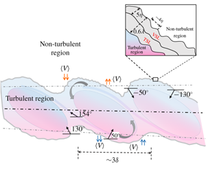
Before we proceed further, it is necessary to point out the difference between a spatial and a temporal mixing layer, which can alter the entrainment characteristics for these two cases. A spatial mixing layer has a non-zero transverse velocity, whereas it is zero for a temporal one. Consistently, the centre of a spatial mixing layer is found to be tilted away from the horizontal $x$-direction, and in our case the tilt is towards the negative $y$-direction, as seen in figure 4(b). Hence, the entrainment is expected to be asymmetric. This is the key difference between the present work and the earlier studies on TNTI.

Following Pope (Reference Pope2000), we define the mean locations of the upper and lower interfaces. The mean upper interface ($y_{0.1}$) is defined as the loci of points where $\overline{U}=U_{2}+0.1U_{d}$. Similarly, the lower interface ($y_{0.9}$) is identified by the location where $\overline{U}=U_{2}+0.9U_{d}$. The mixing layer centre ($y_{0.5}$) is found using $\overline{U}=U_{2}+0.5U_{d}$. The locations of the upper interface, the lower interface and the mixing layer centre are shown in figure 4(b). We find that the mixing layer centre ($(\text{d}y_{0.5}/\text{d}x)=-0.014$) is aligned towards the high-speed side. Furthermore, growth of the upper interface ($|\text{d}y_{0.1}/\text{d}x|=0.009$) is small compared with the lower interface ($|\text{d}y_{0.9}/\text{d}x|=0.034$). The tilt of the mixing layer centre in the negative $y$-direction and a smaller growth rate for the upper interface collectively hints that the lower interface may entrain more compared with the upper interface. However, figure 4(a) shows that magnitude of the transverse velocity is less on the lower side of the mixing layer (negative $\unicode[STIX]{x1D709}$) compared to the upper side (positive $\unicode[STIX]{x1D709}$), indicating perhaps naively more entrainment on the upper side compared to the lower side.

The reason for this discrepancy is due to the fact that we have considered the growth rate of the interfaces in a laboratory frame of reference. Instead, if one fixes the coordinate system along the mixing layer centre, one can define mixing layer thickness for the upper and lower interfaces, $\unicode[STIX]{x1D6FF}_{u}$ and $\unicode[STIX]{x1D6FF}_{l}$, respectively, as illustrated in figure 4(b). The growth rate of these thicknesses is found by fitting a straight line, as shown in figure 4(c). It is observed that the growth rate is slightly higher for the low-speed side of the mixing layer, which is consistent with the literature (e.g. Champagne, Pao & Wygnanski Reference Champagne, Pao and Wygnanski1976). It indicates a higher entrainment along the low-speed side. However, with large coherent structures present along the mixing layer, the instantaneous interface has very large contortions or tilts, and, hence, the mean tilt as such has much smaller magnitude. Therefore, for a detailed understanding of the differences between the upper and lower interfaces, one has to look into the geometric properties of the TNTI, the conditional velocities and length-scales around the interface, as detailed in §§ 4, 5 and 6, respectively.

4.1 Identification of the TNTI

During the entrainment process, the conversion of an irrotational fluid into a turbulent fluid occurs over a region of finite thickness. In various DNS studies (e.g. Bisset et al. Reference Bisset, Hunt and Rogers2002; da Silva & Taveira Reference da Silva and Taveira2010; Watanabe et al. Reference Watanabe, Sakai, Nagata, Ito and Hayase2015), the TNTI is considered as a 2-D surface of zero thickness (identified using a single threshold value of vorticity or scalar concentration) in the 3-D flow field that resides within this finite transition region. However, in planar PIV experiments, only 2-D slices of the velocity data are available. Hence, in this case the TNTI is a line which distinguishes the regions with a very small vorticity (not zero vorticity due to the inherent measurement noise) and regions with relatively higher vorticity (due to turbulence). Identifying the TNTI usually requires a proper choice of a detection criterion and a suitable threshold value. In the present work, TNTI is identified using the absolute value of the spanwise vorticity ($|\unicode[STIX]{x1D714}_{z}|$) as the detector function, which is not common among the experimental community utilizing the planar PIV technique to study TNTI. This is mainly due to the limited spatial resolution of the earlier PIV measurements which may prevent an accurate calculation of vorticity. Therefore, the fluctuating kinetic energy from PIV measurements or the scalar concentration from a simultaneous PIV-LIF measurement has been used as the detection criteria in most of the earlier experiments (e.g. Westerweel et al. Reference Westerweel, Fukushima, Pedersen and Hunt2009; Chauhan et al. Reference Chauhan, Philip, de Silva, Hutchins and Marusic2014b; Mistry et al. Reference Mistry, Philip, Dawson and Marusic2016; Balamurugan et al. Reference Balamurugan, Rodda, Philip and Mandal2018). Because of the relatively high spatial resolution in the present measurements, we have the advantage of using the spanwise vorticity to perform such an analysis. It has also been observed earlier that the spanwise component of vorticity contributes the most to the total vorticity in a shear layer (e.g. Jahanbakhshi et al. Reference Jahanbakhshi, Vaghefi and Madnia2015), and the conditional profiles with respect to the TNTI location obtained using spanwise vorticity as the TNTI detector are almost identical to those obtained using the absolute vorticity magnitude (Watanabe, Zhang & Nagata Reference Watanabe, Zhang and Nagata2018). Hence, we assume that the TNTI identified using the absolute spanwise vorticity propitiously follows the one found using total vorticity. In the following, a simple use of the term vorticity signifies the spanwise component of it.

Figure 5. Illustration of the area algorithm used to find the vorticity threshold using a sample case. (a) An instantaneous PIV realization taken from case M2C1 shows contours of absolute vorticity and the TNTI identified for a given threshold level. Arrows indicate the representative mean velocity vectors of the mixing layer. (b) Definition of upper ($A_{u}$) and lower ($A_{l}$) areas. (c,e) Variation of upper and lower areas with the threshold for cases M2C1 and M1C3, respectively. (d,f) Final threshold detection using a dual-slope method for cases M2C1 and M1C3, respectively. - - - - (red), upper interface; —— (blue), lower interface; —— (black), linear fit to the curve. Dual-slope method to find the value of vorticity threshold corresponding to the point where the linear fit curves intersect: ▴ (red), threshold for the upper interface and ▾ (blue), threshold for the lower interface.

The threshold value of vorticity to identify the TNTI is found following Mistry et al. (Reference Mistry, Philip, Dawson and Marusic2016) based on the empirical process proposed by Prasad & Sreenivasan (Reference Prasad and Sreenivasan1989). The threshold value is identified as that value at which a plot between the turbulent area and the vorticity value used to identify the interfaces displays a distinct slope change. The turbulent region is considered as the area between the upper and lower interfaces, as illustrated in figure 5(a). In calculating the area, small islands of irrotational fluid inside the TNTI and rotational fluid outside the TNTI are excluded. Moreover, Mistry et al. (Reference Mistry, Philip, Dawson and Marusic2016) used a single threshold value to identify both the top and bottom interfaces (see their figure 6). This threshold identification process, although it seems straightforward for a turbulent jet, is not the same for a turbulent mixing layer because the mixing layer is bounded by non-turbulent regions with an ‘asymmetric’ mean free stream velocity. Hence, we expect to obtain two different vorticity thresholds for the upper and lower interfaces of a mixing layer. This asymmetry is tackled by defining two areas based on the irrotational fluid above and below the turbulent region.

The upper area $(A_{u})$ is defined as the region between the upper interface and a horizontal line at the top end of the measurement zone spanning the entire region of interest. This is shown in figure 5(b) as the region occupied by the red contour. Similarly, the lower area ($A_{l}$) is defined as the region between the lower interface and a horizontal line at the bottom, as also shown in figure 5(b) using a blue contour line. The distributions of the upper and lower areas for different threshold values calculated by the above approach and their respective slopes with respect to $\unicode[STIX]{x1D714}_{th}$ are shown in figure 5(c) and (d), respectively. One can observe that, as the threshold value increases, $A_{u}$ and $A_{l}$ increase monotonically and reach a constant value after a particular threshold (figure 5c). The respective slope of these area curves is then plotted and the intersection of linear fits to both the monotonic decrease and nearly constant value regions of the slope curve is chosen as the threshold value, as illustrated in figure 5(d). One can find a clear change of slope at the threshold values of nearly $15~\text{s}^{-1}$ and $16~\text{s}^{-1}$ for the upper and lower interfaces, respectively, for the M2C1 case. Similarly, results for the M1C3 case are shown in figure 5(e–f). As expected, the value of vorticity at which the area changes slope is different for the upper and lower interfaces for the case of a mixing layer. Usually any threshold value within the constant area portion can result in similar conditional profiles in TNTI studies (Bisset et al. Reference Bisset, Hunt and Rogers2002). However, in the present study, the vorticity threshold, $|\unicode[STIX]{x1D714}_{z,th}|$, is chosen as the smallest value of $|\unicode[STIX]{x1D714}_{z}|$ at which the slope changes. This ensures that the TNTI is situated at the outermost part of the interface layer. We may note that only those realizations for which the TNTI spanned the entire measurement region are considered for the TNTI analyses (e.g. Foss et al. Reference Foss, Bade, Neal, Prevost and Morris2017), and the rest are neglected. However, the number of neglected realizations is found to be less than 2 % of the total realizations.

4.2 Geometric properties of the TNTI

The turbulent region in a mixing layer is exposed to two different irrotational regions. The upper side of the mixing layer in the present case is exposed to an irrotational region with lower free stream velocity compared to the turbulent region, and the lower side of the mixing layer is exposed to an irrotational region with higher free stream velocity than the turbulent region, as depicted in figure 5(a) using a sample velocity profile (not to the scale). This might lead to an asymmetry in the flow dynamics between the upper and lower sides of the mixing layer. Hence, unlike the earlier studies, it is worth comparing the geometric properties of the upper and lower TNTIs separately. In this section different geometric features associated with a TNTI such as its transverse location, length, orientation and its curvature are presented. The probability density function (PDF) of the transverse location of the upper and lower interfaces are shown in figure 6(a). The PDF of the upper interface has a peak at $y=0.0128$ m and the mean of the interface location is at $Y_{m,u}=0.0116$ m (shown by the square yellow dot), whereas the PDF of the lower interface has a peak at $y=-0.0125$ m and the interface location has a mean of $Y_{m,l}=-0.0126$ m, which is almost indistinguishable from the peak location. We see that the upper and lower interfaces are on an average symmetrically distributed with respect to the mixing layer centre. Both the PDFs closely follow a Gaussian distribution, as shown by the solid black lines in figure 6(a), although a slight deviation from the Gaussian distribution can be noticed towards the tails. This is consistent with the interfaces identified in other shear flows (e.g. Westerweel et al. Reference Westerweel, Fukushima, Pedersen and Hunt2009).

Figure 6. (a) Probability density function of the interface position, $y_{i}$. Symbols: ◼ (yellow), mean position of the interface; solid lines ——, Gaussian fit for the PDF. (b) Length of the interface, $L_{I}$, normalized with the streamwise length of the data field for different PIV realizations. Symbols: ▵ (red), upper interface; ▿ (blue), lower interface. Cumulative mean of the interface length over consecutive PIV realizations for - - - -, upper and – ⋅ – ⋅ –, lower interfaces. Data are presented for case M1C1.

The interface length $(L_{I})$, obtained from the instantaneous spanwise vorticity fields and normalized by the streamwise extent of the measurement domain, $L_{x}$, is displayed in figure 6(b) for all the PIV realizations utilized for this calculation. The total length is calculated as the cumulative sum of the Euclidean distance between the consecutive interface points from the beginning to the end of the interface. A cumulative average of the length over consecutive realizations, shown as black dashed and dash–dotted lines in figure 6(b), converges to a value of 3.41 and 3.26 for the upper and lower interfaces, respectively. The present values of the average interface length are comparable with those reported by Mistry et al. (Reference Mistry, Philip, Dawson and Marusic2016) and Chauhan et al. (Reference Chauhan, Philip, de Silva, Hutchins and Marusic2014b) for a turbulent jet and a boundary layer, respectively. From figure 6(b) and also from the other cases (not shown here), we find that the mean length of the upper interface is slightly larger than the lower interface for a mixing layer within a confidence level of $95\%$. The close match of lengths with other studies is perhaps fortuitous because the lengths depend on (i) the resolution of the measurement and (ii) the large-scale eddies and (iii) the Kolmogorov length scale in each flow. In any case, the instantaneous length of the interfaces in figure 6(b) varies between two and five times the streamwise extend of the data field, implying that the interfaces are highly convoluted over a range of scales.

Figure 7. A sketch illustrating the different possible interface orientations and interface curvatures depending on the direction and arrangement of the interface unit normal vector, $\hat{\boldsymbol{n}}$. TR (shaded region) and N–TR represents turbulent and non-turbulent parts of the flow. Red arrow indicates the direction of $\hat{\boldsymbol{n}}$. Turbulent region is identified using the direction of the arrow and the grey shade. ‘$+\text{ve}$’, positive and ‘$-\text{ve}$’, negative

The geometric parameters, surface curvature $(\unicode[STIX]{x1D705}_{i})$ and interface orientation $(\unicode[STIX]{x1D703}_{i})$, are illustrated using a simple sketch in figure 7. This figure summarizes different possible interface curvatures and orientations that can occur in the flow field and are pertinent to both the upper and lower interfaces. In both cases the TNTI separates the turbulent (TR) and the non-turbulent (N-TR) regions, and the unit normal vector $\hat{\boldsymbol{n}}$ always points into the turbulent region. The position of the turbulent region is shown using the grey shade for clarity.

The interface orientation ($\unicode[STIX]{x1D703}_{i}$) is defined as the angle between the positive $x$-axis and the interface unit normal, as depicted in figure 7(a). The angle is considered to be positive ($0^{\circ }$ to $180^{\circ }$) if the normal vector lies in the first and second quadrants and its magnitude is measured in the counter-clockwise direction. It is considered negative ($0^{\circ }$ to $-180^{\circ }$) if the normal vector lies in the third and fourth quadrants and its magnitude is measured in the clockwise direction. The PDF of $\unicode[STIX]{x1D703}_{i}$, for the upper and lower interfaces, are shown in figure 8(a). The PDF shows a bimodal distribution both for the upper and lower interfaces, with peaks at $50^{\circ }$ and $130^{\circ }$ for the lower interface, and $-130^{\circ }$ and $-50^{\circ }$ for the upper interface. The peaks have a spacing of $80^{\circ }$ between each other. Another striking feature that one can infer out of the PDF plot is that the orientation of the upper interface is linked with the lower interface, i.e. an angle of $-130^{\circ }$ in the upper interface is associated with an angle of $50^{\circ }$ in the lower interface. Similarly $-50^{\circ }$ for the upper interface is related to $130^{\circ }$ for the lower interface. This interconnection indicates the existence of large-scale structures having a preferential alignment with respect to the flow direction. Using displacement and intermittency correlation plots, Townsend (Reference Townsend1980) also explained that the large-scale eddies are the agents of distortion of the bounding surface in a mixing layer. It will be shown later in § 5.3 that the conditional profiles of the trailing edge of the lower interface is similar to the leading edge of the upper interface. Moreover, the two peaks in the PDF fall within the trailing and the leading edges of the TNTI, respectively. The leading and trailing edges are differentiated using the absolute value of the interface orientation, i.e. $0^{\circ }\leqslant |\unicode[STIX]{x1D703}_{i}|<65^{\circ }$ – trailing edge and $115^{\circ }\leqslant |\unicode[STIX]{x1D703}_{i}|<180^{\circ }$ – leading edge. The positive and negative nature of the orientation angle is due to the coordinate system followed in the present study, in which the normal always points toward the turbulent region. The presence of preferential alignment due to large-scale structures are further consolidated using the linear stochastic estimation in the next section.

Figure 8. Probability density functions of the interface orientation and the interface curvature. Symbols: ▵ (red), upper interface; ▿ (blue), lower interface. Filled symbols, case M2C1; open symbols, case M1C1. (a) PDF of interface orientation. (b) PDF of the interface curvature. Solid line, Gaussian profile fit to the PDF. Inset in (b) is a zoomed-in view and the maximum values of PDFs are highlighted using yellow squares which show the bias towards concave $(-\text{ve})$ curvature. The dashed line shows the zero curvature value. The data are presented only for the case M2C1, for clarity.

The mean curvature of the interface is defined as the rate at which the normal or the tangent vector of the interface changes direction. The expression for the mean curvature is given by

(4.1)$$\begin{eqnarray}\unicode[STIX]{x1D705}_{i}=(\unicode[STIX]{x1D735}\boldsymbol{\cdot }\hat{\boldsymbol{n}})/2,\end{eqnarray}$$

where $\hat{\boldsymbol{n}}=\unicode[STIX]{x1D735}(\unicode[STIX]{x1D714}_{z}^{2})/|\unicode[STIX]{x1D735}(\unicode[STIX]{x1D714}_{z}^{2})|$ is the interface unit normal, defined as the normalized gradient of the spanwise enstropy. Here, the gradient operator ($\unicode[STIX]{x1D735}$) is defined as $[(\unicode[STIX]{x2202}/\unicode[STIX]{x2202}x)\hat{\boldsymbol{e}_{x}}+(\unicode[STIX]{x2202}/\unicode[STIX]{x2202}y)\hat{\boldsymbol{e}_{y}}]$. The unit normal $\hat{\boldsymbol{n}}$, in general, can point along any direction in the 3-D space, but in the present study it is a vector in the 2-D PIV measurement plane. Thus, the analyses presented here are limited to this approximation. Since the interface is highly convoluted and has non-unique points at a single streamwise location, it is difficult to calculate the divergence of the normal $(\hat{\boldsymbol{n}})$ along the interface. However, for a planar curve, the interface curvature can also be found using the parametric form based on the coordinate along the curve. The expression for the curvature in parametric form is given by

(4.2)$$\begin{eqnarray}\unicode[STIX]{x1D705}_{i}=\frac{{\displaystyle \frac{\text{d}x}{\text{d}s}}{\displaystyle \frac{\text{d}^{2}y}{\text{d}s^{2}}}-{\displaystyle \frac{\text{d}y}{\text{d}s}}{\displaystyle \frac{\text{d}^{2}x}{\text{d}s^{2}}}}{\left[\left({\displaystyle \frac{\text{d}x}{\text{d}s}}\right)^{2}+\left({\displaystyle \frac{\text{d}y}{\text{d}s}}\right)^{2}\right]^{3/2}},\end{eqnarray}$$

where $s$ is the parameter along the interface direction (e.g. Mistry et al. Reference Mistry, Philip and Dawson2019). Since the interface points are not increasing monotonically in the streamwise direction, the curvature calculation is done analytically from a polygon fitted to the three point stencil. The PDF of the interface curvature ($\unicode[STIX]{x1D705}_{i}$) for the upper and lower interfaces are shown in figure 8(b). The distribution with wide tails does not follow a Gaussian distribution (as shown with a solid line) implying the importance of higher curvature values (i.e. small scales) on the interface. We find that the peak value of the PDF is at $-0.25\unicode[STIX]{x1D706}$ ($-0.013\unicode[STIX]{x1D702}$) for both the upper and lower interfaces. The negative sign of the mean curvature corresponds to concave surfaces as one views from the turbulent region, and this hints at the presence of vortical structures tangential to the interface inside the turbulent region. Such preference towards concave surfaces are also reported in the DNS studies of temporal jets (Watanabe et al. Reference Watanabe, da Silva, Nagata and Sakai2017) and mixing layer (Jahanbakhshi & Madnia Reference Jahanbakhshi and Madnia2016).

It has also been shown in the temporal DNS studies of turbulent wake (Philip et al. Reference Philip, Bermejo-Moreno, Chung and Marusic2015) and mixing layer (Jahanbakhshi & Madnia Reference Jahanbakhshi and Madnia2016) that the peak value in the PDF of curvature is related to curvedness defined as $\unicode[STIX]{x1D712}=\sqrt{2\unicode[STIX]{x1D705}^{2}-\unicode[STIX]{x1D705}_{g}^{2}}$, which is a measure of the radii ($1/\unicode[STIX]{x1D712}$) of the large-scale structures around the TNTI; here $\unicode[STIX]{x1D705}$ and $\unicode[STIX]{x1D705}_{g}$ denote the mean and the geometric curvature, respectively. In the present case, we are left with only the mean curvature $\unicode[STIX]{x1D705}$ as we cannot explicitly calculate the geometric curvature $\unicode[STIX]{x1D705}_{g}$. Only by substituting the mean curvature value in the curvedness expression, we find a peak radius of ${\approx}3\unicode[STIX]{x1D706}$ to 5$\unicode[STIX]{x1D706}$. Using 3D DNS data, Jahanbakhshi & Madnia (Reference Jahanbakhshi and Madnia2016) found the radius value of around ${\approx}1\unicode[STIX]{x1D706}$ to $1.4\unicode[STIX]{x1D706}$. The slightly higher value of the radius in the present study can be attributed to the omission of $\unicode[STIX]{x1D705}_{g}$ due to the constraints in our 2-D experimental data compared to their fully 3-D DNS data. However, the structures are still found to be of the order of the Taylor microscale within the given limitations.

Therefore, the peaks of the PDFs of both the interface orientation and the curvature indicate signature of the large-scale structures on the TNTI.

4.3 Statistical flow structures around the TNTI

To identify the signature of large-scale structures in a turbulent mixing layer, a vortex identification scheme such as $Q$ or $\unicode[STIX]{x1D706}_{2}$ criteria may not be helpful. This is mainly due to the presence of substantial amounts of small-scale vortices which obscure the identification of large-scale structures. However, conditional averaging based on linear stochastic estimation (LSE) has been utilized to extract the dominant flow structures in different turbulent flows by Adrian and his co-workers (e.g. Adrian et al. Reference Adrian, Jones, Chung, Hassan, Nithianandan and Tung1989; Christensen & Adrian Reference Christensen and Adrian2001). They identified the hairpin vortex organization inside the turbulent boundary layer by conditioning the flow with respect to the swirling strength (Christensen & Adrian Reference Christensen and Adrian2001). The conditionally averaged velocity field ($v_{j}$) for a given conditional variable ($q$) about the reference point $\left(x_{r},y_{r}\right)$ can be estimated linearly as

(4.3)$$\begin{eqnarray}\langle v_{j}(x^{\prime },y^{\prime })|q(x_{r},y_{r})\rangle \approx L_{j}q(x_{r},y_{r}),\end{eqnarray}$$

where $L_{j}$ is the linear estimation coefficient determined by minimizing the mean-square error between the estimate and the conditional average. The mean-square error is minimum if $L_{j}$ is approximated by the two-point spatial correlations between the velocity and the chosen conditional variable. Now conditional averaging is given by

(4.4)$$\begin{eqnarray}\langle v_{j}(x^{\prime },y^{\prime })|q(x_{r},y_{r})\rangle =\frac{\overline{q(x_{r},y_{r})v_{j}(x^{\prime },y^{\prime })}}{\overline{q(x_{r},y_{r})q(x_{r},y_{r})}}q(x_{r},y_{r})\quad \forall \,j=1,2.\end{eqnarray}$$

The symbol $\langle \rangle$ signifies an average over all the realizations and $(x^{\prime },y^{\prime })$ spans over the entire PIV region of interest. Hence, from (4.4), it is apparent that the knowledge of two-point spatial correlations is sufficient to calculate the conditional average. A complete description of the conditional averaging and its relation with the LSE can be found in Adrian (Reference Adrian, Tropea, Yarin and Foss2007).

Figure 9. Autocorrelation contours of $u^{\prime }$ and $v^{\prime }$ velocities showing the signature of large-scale vortices. The mean upper and lower TNTIs are identified as red and blue dashed lines, respectively. The reference point for the autocorrelation is shown as a yellow filled circle at the centre: (a) $R_{u^{\prime }u^{\prime }}$ contour; lines range from 0.1 to 1 in steps of 0.1, where the dashed black line shows the inclination of the $R_{u^{\prime }u^{\prime }}$ contours; (b) $R_{v^{\prime }v^{\prime }}$ contour; lines range from $-0.5$ to 1 in steps of 0.1; the negative contour values are shown as dashed lines. Data are presented for the M1C1 case.

The conditionally averaged $u^{\prime }$ and $v^{\prime }$ can be found by inserting $j=1$ and $j=2$, respectively, in (4.4). Now, we have the 2-D vector field $(u^{\prime },v^{\prime })$ conditioned on the event variable ‘$q$’ occurring at the reference point $(x_{r},y_{r})$. If we choose $q=u^{\prime }$ and $j=1$, we obtain the autocorrelation of $u^{\prime }$, $R_{u^{\prime }u^{\prime }}$ for a unit value of the conditional variable. Similarly, choosing $q=v^{\prime }$ and $j=2$, we obtain the autocorrelation of $v^{\prime }$, $R_{v^{\prime }v^{\prime }}$ for a unit value of the conditional variable. The contours of $R_{u^{\prime }u^{\prime }}$ and $R_{v^{\prime }v^{\prime }}$ about the reference point located at the mixing layer centre (yellow circle) are shown in figure 9. The $R_{u^{\prime }u^{\prime }}$ contours are found to be inclined with respect to the $x$-axis and $R_{v^{\prime }v^{\prime }}$ contours show alternating positive and negative correlations which can be attributed to the presence of the large-scale inclined Kelvin–Helmholtz (K–H) vortical motions. For the above results, the reference point was chosen close to the mixing layer centre so that an overall signature of the flow field, including both the upper and lower interfaces, is obtained. The inclination angle of the $R_{u^{\prime }u^{\prime }}$ contour is found by connecting the two end points of the contour line by a straight line passing through the centre, as shown using the black dashed line in figure 9(a). The contours are inclined at an angle of around $154^{\circ }$ with respect to the flow direction measured in the anti-clockwise direction. From a quick glance over the mixing layer literature, it can be deduced that this inclination angle is due to the braid structures connecting the two consecutive K–H vortices (e.g. Mashayek & Peltier Reference Mashayek and Peltier2012). However, this angle is not close to the peaks in the PDF of $\unicode[STIX]{x1D703}_{i}$ in figure 8(a), because the interface usually resides away from the centre. If one instead takes the reference point at the average interface location then the $R_{u^{\prime }u^{\prime }}$ contours (not shown here) do not reveal any preferential orientation. Hence, it can be concluded that the effect of the braid region is dominant only at the mixing layer centre.

Figure 10. (a–c) Conditionally averaged fluctuating velocity field for a given transverse velocity at different reference points, as identified by yellow squares. The mean locations of the upper and lower interfaces are identified as red and blue dashed lines, respectively. The centres of the large vorticity structures are shown using filled circles. (a) The reference point located at the mean upper interface. (b) The reference point located at the mean lower interface. (c) The reference point located at the mixing layer centre. Solid lines, ranging from 0.2 to 1 in steps of 0.1, indicate contours of $R_{u^{\prime }u^{\prime }}$. (d) Fluctuating velocity vectors over $v^{\prime }$ contours indicate the presence of large vorticity structures along the TNTI, as explicitly shown in the inset figures. The TNTI is identified as a solid black line. Data are presented for the M1C1 case.

The conditional flow structures at the TNTI are obtained by conditioning the flow for a given transverse flow velocity (i.e. $q=v^{\prime }$) at a given reference location. As the entrainment of irrotational flow from the non-turbulent region to the turbulent region occurs predominantly in the transverse direction across the interface, the transverse velocity can be a suitable conditional variable for identifying the conditional structures at the interface. The sign of the velocity does not play a major role as it just changes the direction of the arrows of the conditional velocity field. Assigning $j=1,2$ and $q=-v^{\prime }$, and considering the reference points at the mean upper and lower interfaces, and at the centre of the mixing layer, the conditional velocity fields are calculated and shown in figure 10(a), (b) and (c), respectively. The vectors are normalized by their corresponding magnitude to eliminate the influence of the reference point on the vector length. Correlation contours of $R_{u^{\prime }u^{\prime }}$ are again shown in figure 10(c) for comparison purposes. The conditional vector fields in figure 10(a–c) clearly show two vortices nearly at the mean interface location irrespective of the reference location. These vortices are the structures responsible for the negative $v^{\prime }$ at the reference point $(x_{r},y_{r})$. In fact, such vortices are found to exist even in the instantaneous PIV realizations, as illustrated in figure 10(d); here the $v^{\prime }$ contours also indicate the presence of alternate positive and negative fluctuations similar to the $R_{v^{\prime }v^{\prime }}$ contours shown in figure 9(b). However, the radius of these conditional vortices, obtained using the radius of gyration formula suggested by Bohl & Koochesfahani (Reference Bohl and Koochesfahani2009), is found to be of the order of the Taylor microscale. The procedure for the radius calculation is explained in detail in appendix B. In their DNS study on turbulent jets, da Silva & Taveira (Reference da Silva and Taveira2010) reported the presence of a large vorticity structure of the order of the Taylor microscale close to the TNTI from an instantaneous snapshot and the thickness of the TNTI is equal to the radius of these LVS at the edge of the shear layer. The role of these LVS in the entrainment dynamics was reported by Mistry et al. (Reference Mistry, Philip and Dawson2019). Therefore, the present conditional vortices identified using conditional averaging can be considered as the statistical evidence of these large vorticity structures at the mean TNTI location. This conclusion is further supported by the presence of jump, over a region of $O(\unicode[STIX]{x1D706})$, in the conditional profiles of the spanwise vorticity in § 5.1.

Furthermore, the angle made by a straight line connecting the centre (red and blue square dots) of these vortices and the $x$-axis is found to be $138^{\circ }$ while measured in an anti-clockwise direction. This angle is different than the inclination angle of the $R_{u^{\prime }u^{\prime }}$ contours, as clearly seen in figure 10(c). Interestingly, this angle and the angle between the normal to the straight line connecting the centre of these vortices and the $x$-axis, i.e. $138^{\circ }$ and $48^{\circ }$, are close to the peaks in the PDF of the interface orientation, i.e. $130^{\circ }$ and $50^{\circ }$, as seen in figure 8(a). This indicates that the conditional vortices manifest in this asymmetric manner about the centreline, because there is a preferential alignment of the large-scale structures in the flow, as found from the PDFs of the interface orientation.

Figure 11. Interface coordinate system defined for calculating the conditional profiles. The red and blue lines are the outer envelopes for the upper and lower TNTIs, respectively. The directions $y_{u}$ and $y_{l}$ are along the negative of the interface normal $\hat{n}$, i.e. coordinate increasing into the non-turbulent region. $\cdots \cdots$, TNTI (black color); ——, envelope (red and blue color for upper and lower interfaces, respectively). Data are presented for case M2C1. The filled contours in shades of green represent the magnitude of the spanwise component of vorticity, $|\unicode[STIX]{x1D714}_{z}|$.

5.1 Conditional profiles of mean and turbulence velocities

Here, we consider the profiles of different flow variables conditioned with respect to the interface coordinate (see figure 11) rather than the fixed laboratory reference frame. Such a perspective will be helpful in understanding how the flow properties vary locally at the interface. This viewpoint will be completely shielded, if one just looks into the normal cross-stream variation of the properties in a fixed laboratory frame, as shown in figure 3. Because the interface moves randomly about that fixed frame of reference, the influence of the interface on the flow field will be averaged out at that fixed coordinate location. In this section we present the mean and r.m.s. profiles of the streamwise velocity, the transverse velocity and the spanwise vorticity, conditioned with respect to the TNTI location. The influence of different geometric features on the conditional profiles is discussed in § 5.3.

As the interface is highly contorted, there can be instances where the interface will cross a single streamwise location back and forth. Consistent with others (e.g. Bisset et al. Reference Bisset, Hunt and Rogers2002; Westerweel et al. Reference Westerweel, Fukushima, Pedersen and Hunt2009; Chauhan et al. Reference Chauhan, Philip, de Silva, Hutchins and Marusic2014b; Kwon et al. Reference Kwon, Philip, de Silva, Hutchins and Monty2014), we employ the ‘upper envelope’ of the TNTI, i.e. we choose the farthest transverse location of the interface from the mixing layer centre, which provides a unique interface point (single $y$-location) at every $x$-location. This also ensures that the interface completely encloses the turbulent fluid within it. Moreover, there can be islands/pockets of irrotational fluid inside the interface envelope. Such islands are neglected in the analysis of conditional profiles. This approach has also been followed in many earlier experimental and numerical works (e.g. Bisset et al. Reference Bisset, Hunt and Rogers2002; Westerweel et al. Reference Westerweel, Fukushima, Pedersen and Hunt2009). We note parenthetically that the choice of the ‘upper’ or ‘lower’ envelopes does not make any significant change to the results (e.g. Kwon et al. Reference Kwon, Philip, de Silva, Hutchins and Monty2014). The interface coordinate for either the upper interface $(x_{u},y_{u})$ or lower interface $(x_{l},y_{l})$ has its origin at the interface envelope and is directed along the interface unit normal. The coordinate is assigned positive away from the interface into the non-turbulent region. A sample PIV realization with the identified TNTIs (dotted line) for the given threshold and its farthest envelope (red and blue lines), along with the interface coordinate system used for the conditional profile calculation is shown in figure 11.

Data for the conditional profiles are sampled at equal distances from the interface envelope. The conditional mean profiles were obtained by averaging the extracted data along all the interface points and across all the realizations. The mean streamwise and transverse velocities in the interface coordinates are denoted by $\langle U\rangle$ and $\langle V\rangle$, respectively. The velocity fluctuations with respect to the conditional mean are denoted by $\tilde{u} (=u-\langle U\rangle )$ and $\tilde{v}(=v-\langle V\rangle )$; similarly, the vorticity fluctuations are denoted by $\tilde{\unicode[STIX]{x1D714}}(=\unicode[STIX]{x1D714}-\langle \unicode[STIX]{x1D6FA}\rangle )$.

The conditional profiles of the mean streamwise velocity, the mean transverse velocity and the mean spanwise vorticity are shown in figure 12(a–c). There is a clear jump in the conditional streamwise velocity profile as we approach from the irrotational to the rotational side of the interface (see figure 12a). Moreover, the jump is similar for both the upper and lower interfaces, identified using the ▵ (red) and ▿ (blue) symbols, respectively. The jump in velocity is consistent with previously reported results in other flows (e.g. Westerweel et al. Reference Westerweel, Hofmann, Fukushima and Hunt2002; Chauhan et al. Reference Chauhan, Philip, de Silva, Hutchins and Marusic2014b; da Silva et al. Reference da Silva, Hunt, Eames and Westerweel2014).

Figure 12. Conditional velocity and vorticity profiles. Symbols: ▵ (red), upper interface; ▿ (blue), lower interface. Data are presented for case M1C1. (a) Conditional mean profiles of the streamwise velocity, (b) the transverse velocity and (c) the spanwise vorticity. (d) Conditional r.m.s. profiles of the streamwise velocity (filled symbols) and the transverse velocity (open symbols). (e) Conditional Reynolds shear stress profiles. (f) Conditional r.m.s. profiles of the spanwise vorticity, plotted in interface coordinates $y_{u},y_{l}$ normalized by the Taylor microscale, $\unicode[STIX]{x1D706}$.

The transverse velocity profiles in the interface coordinate system for the upper and lower interfaces are shown in figure 12(b). We can see that the profile switches trend between the upper and lower interfaces at the interface location. This is due to the fact that the irrotational fluid (which gains vorticity) is drawn towards the centre and the turbulent fluid (which transports vorticity) is taken away from the centreline of the mixing layer by viscous diffusion. This point is further consolidated in § 5.2, using the conditional profiles of the 2-D surrogate of the viscous diffusion term in the enstropy transport equation. From the DNS of an incompressible shear layer at a Mach number of 0.2, Jahanbakhshi & Madnia (Reference Jahanbakhshi and Madnia2018a) recently reported a similar transverse velocity distribution. But in their case, the profiles are symmetric with respect to the $\langle V\rangle =0$ location, as their mixing layer develops temporally opposed to the present spatial evolution.

Figure 12(b) also shows that the jump in the transverse velocity is different for the top and bottom interfaces and the jump is high for the upper interface, and it is found to be consistent for all the cases considered in this study. This may be attributed to the asymmetric nature of entrainment for the case of a spatially developing turbulent mixing layer. Another interesting feature to note from the conditional transverse velocity profile is that the value of the transverse velocity is always negative for both the upper and lower interfaces. This might appear as if the upper interface is favouring the motion of irrotational fluid into the turbulent region, but the lower interface is opposing such a motion which is also consistent with the ensemble averaged transverse velocity profile shown in figure 4(a). But the growth of the shear layer, as shown in figure 4(c), reveals that even the lower interface must entrain fluid and grow in the streamwise direction. The conditional profiles of the spanwise vorticity in figure 12(c) show that the vorticity value is almost zero in the non-turbulent region followed by a jump at the interface before settling to a constant value inside the turbulent region.

Figure 12(d,e) shows the conditional profiles of the Reynolds stress components and figure 12(f) shows the conditional profiles of the fluctuating vorticity. Similar to the conditional mean profiles, a jump can be observed while approaching from the irrotational side of the interface. A non-zero value of the Reynolds normal stress outside the interface, as seen in figure 12(d), is attributed to the background noise resulting mainly from the mixing layer mesh and the tunnel free stream turbulence. However, the profiles show similar variation for both the upper and lower interfaces.

The conditional mean and r.m.s. profiles of the velocity and the spanwise vorticity clearly indicate the presence of a jump over a region of finite thickness which is due to the presence of an interface layer. The ordinates of the conditional mean and r.m.s. of the spanwise vorticity plot (see figure 12c,f) are normalized by $\unicode[STIX]{x1D706}$, and it clearly shows the TNTI thickness to be of $O(\unicode[STIX]{x1D706})$. This observation is consistent with the results reported in a number of earlier studies in other free and wall-bounded shear flows (e.g. Westerweel et al. Reference Westerweel, Fukushima, Pedersen and Hunt2009; da Silva & Taveira Reference da Silva and Taveira2010; Chauhan et al. Reference Chauhan, Philip, de Silva, Hutchins and Marusic2014b). As mentioned in the introduction, this layer is further subdivided into a viscous superlayer and a turbulent sublayer (e.g. da Silva et al. Reference da Silva, Hunt, Eames and Westerweel2014; Watanabe et al. Reference Watanabe, da Silva, Sakai, Nagata and Hayase2016). Due to the limitations in their measurements, Chauhan et al. (Reference Chauhan, Philip, de Silva, Hutchins and Marusic2014b) referred to this combined region (containing the VSL and TSL) as a turbulent superlayer. Since the resolution of the present measurements (albeit in two dimensions) is comparable with the DNS of da Silva & Taveira (Reference da Silva and Taveira2010), an attempt has been made to investigate the presence of a viscous superlayer, as discussed in the next section.

5.2 Viscous superlayer

We recall that the viscous superlayer is defined as a thin region in the outer edge of the TNTI, where the viscous diffusion dominates over the turbulent production (Corrsin & Kistler Reference Corrsin and Kistler1955). Based on the relative magnitude of the conditional profiles of the different terms in the enstropy transport equation, a number of DNS studies have recently revealed the existence of a VSL in turbulent jets (Taveira & da Silva Reference Taveira and da Silva2014) and mixing layers (Watanabe et al. Reference Watanabe, Sakai, Nagata, Ito and Hayase2015). However, the presence of such a layer is yet to be reported experimentally in a planar mixing layer mainly due to the absence of highly resolved 3-D velocity data in both space and time. For an incompressible flow, the enstropy transport equation is given by

(5.1)$$\begin{eqnarray}\frac{\text{D}}{\text{D}t}\left(\frac{1}{2}\unicode[STIX]{x1D714}_{i}\unicode[STIX]{x1D714}_{i}\right)=\unicode[STIX]{x1D714}_{i}\unicode[STIX]{x1D714}_{j}S_{ij}+\unicode[STIX]{x1D708}\frac{\unicode[STIX]{x2202}^{2}}{\unicode[STIX]{x2202}x_{j}\unicode[STIX]{x2202}x_{j}}\left(\frac{1}{2}\unicode[STIX]{x1D714}_{i}\unicode[STIX]{x1D714}_{i}\right)-\unicode[STIX]{x1D708}\frac{\unicode[STIX]{x2202}\unicode[STIX]{x1D714}_{i}}{\unicode[STIX]{x2202}x_{j}}\frac{\unicode[STIX]{x2202}\unicode[STIX]{x1D714}_{i}}{\unicode[STIX]{x2202}x_{j}},\end{eqnarray}$$

where $\unicode[STIX]{x1D708}$ is the kinematic viscosity. The left-hand side of the equation is the total rate of change of enstropy. The first, second and third terms on the right-hand side represent enstropy production, viscous diffusion and viscous dissipation, respectively. The numerical works of da Silva et al. (Reference da Silva, Hunt, Eames and Westerweel2014) and Watanabe et al. (Reference Watanabe, da Silva, Sakai, Nagata and Hayase2016) have revealed that the contribution of viscous diffusion exceeds the turbulent production inside the VSL. Since the resolution of the present PIV measurements is comparable with those numerical studies reported above, an attempt is made to identify the VSL with the available 2-D PIV data. From our 2-D PIV measurements, we have access to only one component of vorticity $\unicode[STIX]{x1D714}_{z}(x,y)$ in the $x$–$y$ plane. Therefore, calculation of the enstropy production term is not possible. However, the 2-D surrogates of the diffusion term $D_{f}=\unicode[STIX]{x1D708}(\unicode[STIX]{x2202}^{2}/\unicode[STIX]{x2202}^{2}x)(\frac{1}{2}\unicode[STIX]{x1D714}_{z}\unicode[STIX]{x1D714}_{z})+\unicode[STIX]{x1D708}(\unicode[STIX]{x2202}^{2}/\unicode[STIX]{x2202}^{2}y)(\frac{1}{2}\unicode[STIX]{x1D714}_{z}\unicode[STIX]{x1D714}_{z})$ as well as the dissipation term $D_{s}=-\unicode[STIX]{x1D708}((\unicode[STIX]{x2202}\unicode[STIX]{x1D714}_{z}/\unicode[STIX]{x2202}x)(\unicode[STIX]{x2202}\unicode[STIX]{x1D714}_{z}/\unicode[STIX]{x2202}x)+(\unicode[STIX]{x2202}\unicode[STIX]{x1D714}_{z}/\unicode[STIX]{x2202}y)(\unicode[STIX]{x2202}\unicode[STIX]{x1D714}_{z}/\unicode[STIX]{x2202}y))$ can be estimated from our measured data.

Figure 13. (a) Conditional profiles of the 2-D surrogate of the normalized diffusion term in the enstropy transport equation (5.1). (b) Conditional profiles of the correlation coefficient between the diffusion and the dissipation terms. The distance from the interface ($y_{u}$ and $y_{l}$) is normalized by the Taylor microscale $\unicode[STIX]{x1D706}$ (shown along the left side) and Kolmogorov length scale $\unicode[STIX]{x1D702}$ (shown along the right side). The yellow shaded regions show the extent of the viscous superlayer for both (a,b). Case details for both (a,b): ○, M1C1; ▵, M1C2 and ▿, M1C3; grey filled red and open blue symbols signify the upper and lower interfaces, respectively.

In figure 13(a) we show the conditional profiles of the viscous diffusion term ($D_{f}$) of the enstropy transport (5.1) for the M1C1, M1C2 and M1C3 cases. It is observed that the profile has a peak at a constant location close to the TNTI. As one moves from the irrotational to the turbulent region across the TNTI, the normalized value of the diffusion term increases and reaches a maximum positive value close to the TNTI; then it reduces and reaches a negative minimum before settling to a value close to zero for all the cases. This observation is similar to the one reported by Taveira & da Silva (Reference Taveira and da Silva2014) (see the inset of their figure 1a). According to the detection criteria defined by Taveira & da Silva (Reference Taveira and da Silva2014), the viscous superlayer is identified as the region close to the TNTI where the viscous diffusion term is greater than the turbulent production term. They also reported that the enstropy production term is zero inside the irrotational region, and then its value increases and overtakes the diffusion term just after the peak positive diffusion value. Hence, the distance between the points within which the diffusion value increases from nearly a zero irrotational value to the peak positive value can be considered as an approximate estimate of the viscous superlayer thickness. The advantage with this definition is that it can be used even if the production term is not available as in the case of 2-D PIV measurements. In the present study, the positive diffusion peak is obtained at a distance of about $6\unicode[STIX]{x1D702}$ from the zero diffusion value, as shown by the yellow shaded region in figure 13(a). This value compares well with those reported in the literature (Taveira & da Silva Reference Taveira and da Silva2014; Jahanbakhshi & Madnia Reference Jahanbakhshi and Madnia2016). This result is further substantiated using the correlation analysis of the diffusion and the dissipation terms, as detailed below. The close resemblance between the present result obtained from the 2-D PIV data and the result from the 3-D DNS data of Taveira & da Silva (Reference Taveira and da Silva2014) and Jahanbakhshi & Madnia (Reference Jahanbakhshi and Madnia2016) is attributed to the fact that the diffusion of the spanwise component of vorticity dominates the total vorticity close to the TNTI (Bisset et al. Reference Bisset, Hunt and Rogers2002). It is also found that the VSL thickness is constant for all the cases presented here.

Since only the diffusion and the dissipation terms dominate the total rate of change of enstropy within the viscous superlayer, Jahanbakhshi & Madnia (Reference Jahanbakhshi and Madnia2018b) recently proposed a method to calculate the VSL thickness by plotting the correlation between these terms in the interface coordinate system. The correlation coefficient between the diffusion $(D_{f})$ and dissipation $(D_{s})$ terms is defined as $\langle C(D_{f},D_{s})\rangle =\langle \tilde{D}_{f}\cdot \tilde{D_{s}}\rangle /[\langle \tilde{D}_{f}^{2}\rangle \cdot \langle \tilde{D}_{s}^{2}\rangle ]^{0.5}$, where $\tilde{D}_{f}$ and $\tilde{D}_{s}$ are the fluctuations with respect to the mean values in the interface coordinate. The conditional profiles of $C(D_{f},D_{s})$, calculated from the 2-D surrogate of the diffusion and the dissipation terms, for the upper and lower interfaces, are shown in figure 13(b). The correlation is negative because of the difference in the sign between the two terms in the enstropy transport equation (5.1). The VSL is identified as the region with a correlation value above a certain threshold, $C_{th}$. Similar to Jahanbakhshi & Madnia (Reference Jahanbakhshi and Madnia2018b), a threshold value of 0.8 is used in the present study as well, and based on the above threshold, the thickness of the VSL is found to be around $5\unicode[STIX]{x1D702}$. This value compares well with those obtained from the conditional profile of $\langle D_{f}\rangle$, thereby substantiating the above definition. This is found to be an interesting finding in the present work, as we have used only one component of vorticity to calculate both the diffusion and the dissipation terms, and the values obtained here compare well with those reported in the numerical simulations (Attili et al. Reference Attili, Cristancho and Bisetti2014; Watanabe et al. Reference Watanabe, Sakai, Nagata, Ito and Hayase2015; Jahanbakhshi & Madnia Reference Jahanbakhshi and Madnia2018b), where full 3-D data were employed.

5.3 Effect of geometric parameters on the conditional profiles

The dependence of the conditional profiles, discussed in § 5.1, on various geometric features associated with the TNTI, such as curvature, transverse location and orientation, was investigated. We found that the orientation angle has the maximum influence on the conditional profiles. Hence, we present only the conditional profiles of the streamwise and transverse velocities conditioned based on the orientation angle of the TNTI. This might also shed light into the role of the top and bottom interfaces in flow dynamics around the TNTI. Based on the value of the interface angle ($\unicode[STIX]{x1D703}_{i}$) faced by the interface normal ($\hat{\boldsymbol{n}}$) with the flow direction ($x$) (as schematically illustrated in figure 7), the interface points are divided into:

$$\begin{eqnarray}\displaystyle 0^{\circ }\leqslant |\unicode[STIX]{x1D703}_{i}|<65^{\circ } & : & \displaystyle \text{trailing edge;}\nonumber\\ \displaystyle 65^{\circ }\leqslant |\unicode[STIX]{x1D703}_{i}|<115^{\circ } & : & \displaystyle \text{transverse edge;}\nonumber\\ \displaystyle 115^{\circ }\leqslant |\unicode[STIX]{x1D703}_{i}|<180^{\circ } & : & \displaystyle \text{leading edge.}\nonumber\end{eqnarray}$$

These definitions are similar to the works of Watanabe et al. (Reference Watanabe, Sakai, Nagata, Ito and Hayase2014) and Bisset et al. (Reference Bisset, Hunt and Rogers2002) for the case of a turbulent jet. The absolute value of the angle is considered because leading and trailing edges can be identified using both positive and negative angles. Using an instantaneous PIV realization, the TNTI divided based on the above classification is illustrated in figure 14(a). The TNTI shown in this figure is obtained from a filtered field, which reduces the contortions and makes it easier for illustration. However, we may mention that no data filtering has been carried out in the analyses of the results presented below.

Figure 14. (a) Interface classification based on different geometric features. Vectors which are the interface normal vectors obtained from the gradient of the spanwise enstropy are coloured based on the interface orientation. Conditional profiles of the mean streamwise velocity (b) and the transverse velocity (c) further conditioned with interface orientation. Top interface – different shades of red. Bottom interface – different shades of blue. Data are presented for case M1C1.

Before we present the conditional profiles, the relative contribution of the leading edge, trailing edge and transverse edge type of interfaces to the total interface is reported in table 3. The upper interface is found to be dominated by the leading edge type and the lower interface is dominated by the trailing edge type interface points. This observation is consistent for all the velocity ratios considered in the present study and it is presumed to be an imprint of large-scale structures on the TNTI geometry in the case of a turbulent mixing layer.

Table 3. Percentage of interface orientation angle along the interface. Case detail: M1C1 – mesh 1 case 1, and so on. The lower interface data are tabulated inside the parenthesis.

Using the interface envelope, as shown in figure 11, the conditional profiles are calculated for each range of the interface orientation. The conditional profiles of the streamwise velocity, as shown in figure 12, are further conditioned based on the interface orientation $(\unicode[STIX]{x1D703}_{i})$ and represented as $\left<U\right>_{\unicode[STIX]{x1D703}_{i}}$. Similarly, the profiles of the transverse velocity are represented accordingly. The top interface is identified with different shades (dark, light and lighter) of red and the bottom interface, respectively, by different shades of blue.

The influence of the orientation angle $\unicode[STIX]{x1D703}_{i}$ on the conditional $\langle U\rangle$ is shown in figure 14(b), and we see that the region of the interface oriented along the leading edge of the upper interface and the trailing edge of the lower interface exhibits a maximum jump normal to the interface. Unlike the streamwise velocity, the transverse velocity profile is found to have an appreciable dependence on the interface orientation. In figure 14(c) we show that, for both the upper and lower interfaces, the transverse edge displays the minimum transverse velocity jump. This shows that the flow is predominantly inclined in the streamwise direction along these surfaces. Hence, their influence is not observed in the transverse velocity. The role played by the leading and trailing edges can be understood better if one treats them as parts of a single large entity. For the upper interface, the leading and trailing edges correspond to the segments in figure 7(c) and (d), respectively. Similarly, for the lower interface, the leading and trailing edges correspond to the part of the segments in figure 7(b) and (a), respectively. For the upper interface, the trailing edge portion of the interface has larger negative transverse velocity compared with the transverse edge. The leading edge has a peak positive transverse velocity opposite to that of the trailing and transverse edges. Similarly, for the lower interface, the trailing edge portions of the interface have a peak negative transverse velocity, i.e. a fluid movement away from the turbulent region and the leading edge portions show a peak positive transverse velocity close to the TNTI, i.e. a fluid movement towards the turbulent region. The positive and negative transverse velocities associated with the leading and trailing edges, respectively, at both the upper and lower TNTIs indicate the presence of a vortex with counter-clockwise rotation propagating along the flow direction. This counter-clockwise vortex is due to the signature of K–H rolls, that are still dominant, at such downstream locations, in the case of a turbulent mixing layer.

6.1 Multi-scale characteristics of the TNTI

To substantiate that the entrainment occurs at different ranges of length scales (Townsend Reference Townsend1980) in a TNTI, Sreenivasan & Meneveau (Reference Sreenivasan and Meneveau1986) reported that the TNTI must have a geometric nature similar to a fractal object. Such an object will have a characteristic dimension called the fractal dimension ($D_{3}$) different from its Euclidean dimension (which is zero for a point, 1 for a line and so on). The value of the fractal dimension ($D_{3}$) for a 3-D TNTI surface was reported to be within the range of 2.3–2.4 and it can be obtained using the box counting method (e.g. Prasad & Sreenivasan Reference Prasad and Sreenivasan1989; de Silva et al. Reference de Silva, Philip, Chauhan, Meneveau and Marusic2013; Mistry et al. Reference Mistry, Philip, Dawson and Marusic2016) and the data filtering approach (e.g. Mistry et al. Reference Mistry, Philip, Dawson and Marusic2016). In the box counting method the number of square boxes $(N)$ required to cover the TNTI completely is plotted against the box size ($\unicode[STIX]{x1D6E5}_{b}$) on a log–log graph, as shown in figure 15(a). The 2-D fractal dimension ($D_{2}$) is then given by the slope of a curve fitted within the range of box sizes constrained by experimental conditions such as $Re$, spatial resolution and the length scales present in the flow. The limits of the range are detected using a compensated plot, as shown in the inset of figure 15(a), where the region within which the slope of the curve remains constant is chosen for fitting the power-law curve. For the present case, the limits are found to be approximately $5\unicode[STIX]{x1D702}$–$0.5\unicode[STIX]{x1D6FF}$, as shown using blue and yellow dashed lines in figure 15(a). A fractal dimension, $D_{2}\approx 1.3$, is obtained for both the upper and lower interfaces for all the cases reported in this study. The corresponding fractal dimension for a 3-D interface is given by $D_{3}=D_{2}+1\approx 2.3$ (Mandelbrot Reference Mandelbrot1982), which is close to the values obtained in other free and wall-bounded shear flows. Another complementary way to establish the fractal nature of a TNTI is by showing that the interface length obtained from the filtered velocity data scales with the filter width (Mistry et al. Reference Mistry, Philip, Dawson and Marusic2016). The length of the interface is found from the TNTIs identified by applying the same threshold to the vorticity data obtained from the spatially filtered velocity field. Spatial filtering of the velocity data is performed using a 2-D box filter of size $\unicode[STIX]{x1D6E5}_{f}$, commonly used in large-eddy simulations of turbulent flows (see de Silva et al. (Reference de Silva, Philip, Chauhan, Meneveau and Marusic2013) for details). Logarithmic plot of the interface length, ensemble averaged over all data sets, against the filter width is shown in figure 15(b). A dashed line with a slope of $-0.4$ is also plotted and it is found to fit the data between the filter width of size $0.8\unicode[STIX]{x1D706}$ and $1.2\unicode[STIX]{x1D706}$. This indicates a power-law scaling for length $L\sim \unicode[STIX]{x1D6E5}_{f}^{-D}$ with a fractal dimension of $D_{2}=D+1\approx 1.4$ (Mandelbrot Reference Mandelbrot1982). The results are found to be similar to other shear flows (de Silva et al. Reference de Silva, Philip, Chauhan, Meneveau and Marusic2013; Mistry et al. Reference Mistry, Philip, Dawson and Marusic2016) with slight differences between the upper and lower interfaces (see figure 15b). Overall, we can infer from the current analysis that TNTIs for all the shear flows in the self-similar region share similar fractal properties within the range of resolved length scales in the flow. This indicates that a range of length scales take part in the flow dynamics, and, hence, on the entrainment, close to the TNTI.

Figure 15. Fractal characteristics of the TNTI. (a) Box counting method: fractal dimension obtained as the slope of the fit to the log–log plot between the box size $\unicode[STIX]{x1D6E5}_{b}$ and the number of square boxes $N$ required to span the TNTI. The inset in the figure is a compensated plot showing the local slope of the points with respect to the box size. We see that the inertial scaling is possible between the box sizes of the order of $5\unicode[STIX]{x1D702}$–$0.5\unicode[STIX]{x1D6FF}$, shown using blue and yellow dashed vertical lines. (b) Spatial filtering method: log–log plot of the filter size $\unicode[STIX]{x1D6E5}_{f}$ and the interface length $L_{I}$. The fractal dimension is obtained from the exponent of the power-law fit (i.e. slope of the dashed line). Here $L_{x}$ is the streamwise extent of the measurement domain and $\unicode[STIX]{x1D706}$ is the Taylor microscale. Symbols: ▸ (red/filled), upper interface; ▹ (blue/open), lower interface. The data are presented for case M1C1.

6.2 Thickness of the TNTI

Dominant length scales associated with the TNTI can be found by various approaches, for example, using the spatial correlation of a flow variable along the TNTI (e.g. Westerweel et al. Reference Westerweel, Fukushima, Pedersen and Hunt2005; Chauhan et al. Reference Chauhan, Philip, de Silva, Hutchins and Marusic2014b). A simple straightforward approach to determine the order of the TNTI thickness is to look into the conditional profiles of the spanwise vorticity in the interface coordinates as shown in figure 12(c). From the conditional vorticity profiles, the thickness of the TNTI can be defined as the width of the region starting at the TNTI $(y-y_{i}=0)$ to the location where vorticity reaches a peak value inside the turbulent region. This thickness is related to the radius of the large vorticity structure alongside the TNTI (da Silva & Taveira Reference da Silva and Taveira2010). This value in experiments is found to be of the order of the Taylor microscale in turbulent jets (Westerweel et al. Reference Westerweel, Fukushima, Pedersen and Hunt2009; Mistry et al. Reference Mistry, Philip, Dawson and Marusic2016) and shear layers (Jahanbakhshi et al. Reference Jahanbakhshi, Vaghefi and Madnia2015), and of the order of the Kolmogorov length scale for the turbulence generated by an oscillating grid (Holzner & Lüthi Reference Holzner and Lüthi2011). Based on the above definition, we can observe a clear peak in figure 12(c). In the present study the TNTI thickness for the upper and lower interfaces from the conditional vorticity profiles is found to be around 0.6 times the Taylor microscale, i.e. it is of the order of $\unicode[STIX]{x1D706}$, similar to a turbulent jet (Westerweel et al. Reference Westerweel, Fukushima, Pedersen and Hunt2009), thereby confirming the result proposed by Taveira & da Silva (Reference Taveira and da Silva2014), that the TNTI scales with $\unicode[STIX]{x1D706}$ for flows with mean shear. The thickness of the TNTI based on the conditional vorticity profile are given in table 4 for all the cases considered in this work. The thickness values vary between 0.45 and 0.65 times the Taylor microscale. Furthermore, we cannot discern a difference in thickness between the upper and lower interfaces which is in contrast to the DNS results of a mixing layer by Attili et al. (Reference Attili, Cristancho and Bisetti2014), who reported a higher value of interface thickness along the high velocity side based on the conditional spanwise vorticity (see their figures 6 and 12). However, the thickness is still of the order of $\unicode[STIX]{x1D706}$ in both these studies.

For planar turbulent jets, Silva et al. (Reference Silva, Zecchetto and da Silva2018) found that the thickness of the TNTI scales with the Kolmogorov length scale beyond a threshold Reynolds number, $Re_{\unicode[STIX]{x1D706}}\gtrsim$ 200. The range of $Re_{\unicode[STIX]{x1D706}}$ (135–187) in the present study is below the abovementioned threshold, and therefore, it cannot be ascertained whether such a scaling exists in the present mixing layer. However, any differences that might exist are due to the fact that Silva et al. (Reference Silva, Zecchetto and da Silva2018) could calculate $\unicode[STIX]{x1D706}$ and $\unicode[STIX]{x1D702}$ directly from their 3-D DNS data without invoking the isotropic assumption, whereas the isotropic assumption has been used in the present study to calculate $\unicode[STIX]{x1D706}$ and $\unicode[STIX]{x1D702}$ from our 2-D PIV data. Furthermore, the magnitude of the vorticity vector containing all three components was used in the work of Silva et al. (Reference Silva, Zecchetto and da Silva2018), whereas we have used only its spanwise component while calculating the vorticity threshold and the TNTI thickness from the conditional vorticity profiles. Nonetheless, given the experimental constraints in the present work, the TNTI thickness is found to be ${\approx}0.5$ times the Taylor microscale and an order of magnitude (around 10–16 times) larger than the Kolmogorov length scale, consistent with the results of Bisset et al. (Reference Bisset, Hunt and Rogers2002).

Table 4. Thickness of the TNTI using the conditional profiles of spanwise vorticity. The values are normalized with the corresponding Taylor microscale, $\unicode[STIX]{x1D706}$ and those inside the parentheses are normalized by the Kolmogorov length scale, $\unicode[STIX]{x1D702}$, of the respective cases.

6.3 Length scale based on correlation analysis

The analysis in § 6.1 clearly indicates that there exists a range of scales along the TNTI. One dominant length scale at the TNTI is its thickness, as reported in § 6.2. For a further detailed understanding of the length scales responsible for the fluctuations in the TNTI or the fluctuations of the flow variables along the TNTI, Chauhan et al. (Reference Chauhan, Philip, de Silva, Hutchins and Marusic2014b) and Westerweel et al. (Reference Westerweel, Fukushima, Pedersen and Hunt2005) proposed the usage of spatial autocorrelation of different flow variables along the TNTI. Although correlation based methods seem to be straightforward, it has a drawback while applying to a TNTI mainly because of the highly fluctuating nature of the TNTI. The $x$-location of the interface is not monotonic and the interface folds back and forth onto itself. This restrains one from performing autocorrelation of any flow variable along the $x$-direction. Hence, we have carried out correlation along the interface coordinate defined as ‘$s$’, following Chauhan et al. (Reference Chauhan, Philip, de Silva, Hutchins and Marusic2014b). The autocorrelation function is defined as

(6.1)$$\begin{eqnarray}R_{\tilde{q}\tilde{q}}(r)={\displaystyle \frac{\overline{\tilde{q}(s_{i})\tilde{q}(s_{i}+r)}}{\tilde{q}_{rms}^{2}}},\end{eqnarray}$$

where $\tilde{q}(=q-\langle Q\rangle )$ is the fluctuation of any flow variable with respect to its conditional mean and $r$ is the lag variable in the $s$ direction – the distance along the TNTI. We see in figure 6(b) that the ‘$s$’ and ‘$x$’ coordinates are linked by a common ratio of 3.41 (3.26) for the upper (lower) interface. This ratio can be used to retrieve the scales along the $x$-coordinate. Here, we have considered three different variables $y_{i}$, $u_{n}$ and $\unicode[STIX]{x1D705}_{i}$ for estimating the length scales at the TNTI, where $y_{i}$, $u_{n}(=\boldsymbol{u}\boldsymbol{\cdot }\hat{\boldsymbol{n}})$ and $\unicode[STIX]{x1D705}_{i}$ are the interface transverse location, the normal flow velocity and the interface curvature, respectively.

Figure 16. Length scale calculation using correlation based methods for various cases of mesh 1. (a,b) Correlation curves of different flow variables calculated along the interface coordinates for the upper and lower interfaces, respectively. (c,d) Pre-multiplied power spectra obtained from the discrete cosine transform of the correlation curves in (a,b) for the upper and lower interfaces, respectively. Symbols: ○, M1C1; ▵, M1C2 and ▿, M1C3. Symbol color: blue, curvature ($\tilde{\unicode[STIX]{x1D705}_{i}}$); black, interface normal velocity ($\tilde{u_{n}}$); red, transverse interface location ($\tilde{y_{i}}$). Some of the symbols are skipped for clarity.

From a visual inspection of the TNTI (see figure 11), we can observe that the transverse location, $y_{i}$, shows large-scale oscillation with respect to its mean location. Moreover, from their high-Reynolds-number PIV data in a turbulent boundary layer, Chauhan et al. (Reference Chauhan, Philip, de Silva, Hutchins and Marusic2014b) reported that correlation of the fluctuation of the interface transverse location ($y_{i}$) provides the length scale of the order of the boundary layer thickness. Similarly, from the autocorrelation of the normal velocity fluctuation, they identified the presence of a length scale of the order of the TNTI thickness. We have utilized $\tilde{y_{i}}$ and $\tilde{u_{n}}$ to examine the presence of such similar scales in a planar mixing layer.

In addition, we have chosen the interface curvature ($\tilde{\unicode[STIX]{x1D705}_{i}}$) as another correlation variable to estimate the viscous length scales, as the definition of the interface curvature is intrinsically related to the viscous diffusion of enstropy (see (4.1)). It is found in § 5 that a rapid change in the vorticity diffusion occurs at a distance of the order of the Kolmogorov length scale close to the TNTI (see figure 13a). Moreover, Mistry et al. (Reference Mistry, Dawson, Philip and Marusic2017) reported that the surface curvature of the TNTI tends to be formed by smaller-scale structures that give rise to very sharp contortions, which may be attributed to the small eddies along the interface where viscosity plays a dominant role. As already mentioned earlier, this viscosity dominated region is usually called a viscous superlayer, the thickness of which is found to be of the order of $5\unicode[STIX]{x1D702}$. Furthermore, this region is also found to be dominated by intense vorticity structures (IVS) of size ${\approx}5\unicode[STIX]{x1D702}$ and these structures play an important role in small-scale nibbling (da Silva et al. Reference da Silva, Dos Reis and Pereira2011). These IVS are aligned tangential to the TNTI thereby influencing the curvature of the interface. Hence, the interface curvature is chosen as another parameter signifying the presence of small scales in the vicinity of the TNTI.

Autocorrelation of fluctuations of all three variables are carried along the interface for each realization and averaged over all the realizations. In figure 16(a,b) we show the correlation curves as a function of the lag $\unicode[STIX]{x0394}x$ for the upper and lower interfaces, respectively. One can clearly see that the interface curvature is correlated over a much shorter distance compared to the interface normal velocity and the interface transverse location, reflecting its association with small scales.

Table 5. Details of the normalized length scales obtained from the peak in the pre-multiplied power spectra of the correlation function of interface curvature, interface normal velocity and transverse interface location along the interface coordinates. Case details: M1C1(u) – mesh 1 case 1 upper interface and M1C1(l) – mesh 1 case 1 lower interface, and so on.

The characteristic length scale ($\unicode[STIX]{x1D6EC}_{x}$) associated with each correlating variable ($q$) is found by locating the peak in the amplitude of the pre-multiplied power spectra, as shown in figure 16(c,d) for the upper and lower interfaces, respectively. The pre-multiplied power spectra are obtained from the discrete cosine transform (DCT) of the autocorrelation function similar to Chauhan et al. (Reference Chauhan, Philip, de Silva, Hutchins and Marusic2014b). We can identify the presence of three distinct peaks of the order of the Kolmogorov $(\unicode[STIX]{x1D702})$, Taylor $(\unicode[STIX]{x1D706})$ and integral (mixing layer thickness, $\unicode[STIX]{x1D6FF}$) length scales of the flow for all three cases of mesh 1. These length scales are related to the viscous superlayer (see figure 13), TNTI thickness (see figure 12c) and the streamwise distance between the spanwise roller vortices (see figure 9 and table 2), respectively. A length scale of the order of the viscous superlayer obtained from the curvature looks surprising at first. But it was shown in the DNS of the mixing layer that the curvature has a greater correlation with the viscous diffusion and dissipation terms of the entrainment mass flux equation (Jahanbakhshi & Madnia Reference Jahanbakhshi and Madnia2016). Similarly, it was also observed in flows with and without mean shear (Holzner & Lüthi Reference Holzner and Lüthi2011; Wolf et al. Reference Wolf, Holzner, Lüthi, Krug, Kinzelbach and Tsinober2013) that TNTI curvature is highly correlated to the viscous component of the outward spreading or entrainment velocity of the interface compared to its inviscid component. The length scale of the order of $\unicode[STIX]{x1D702}$ obtained using curvature further consolidates the proposal by Corrsin & Kistler (Reference Corrsin and Kistler1955) that a very thin viscosity dominated layer must be present along the TNTI in which the vorticity is transmitted to the irrotational fluid by the viscous diffusion. This shows that a range of length scales over two orders of magnitude from $\unicode[STIX]{x1D702}$ to $\unicode[STIX]{x1D6FF}$ exists along the TNTI. The length scale values for all the cases considered in the present study are given in table 5 and one may notice that the above conclusions are consistent for all these cases.