


1. Introduction
Supersonic impinging jets have numerous practical applications such as cold additive manufacturing, short take-off and vertical landing aeroplanes, cooling of turbine blades and electronic devices. Under-expanded impinging jets form when the static pressure at the nozzle exit is higher than the ambient pressure. As the jet exit pressure is higher than the surrounding pressure, expansion fans are formed as the boundary of the jet expands. The expansion waves are reflected by the shear layer and form compression waves. The compression fans converge and form a Mach disk (Prandtl Reference Prandtl1904, Reference Prandtl1907; Pack Reference Pack1948). These expansions and contractions form a cellular pattern which is commonly observed in schlieren visualisations of this flow (Risborg & Soria Reference Risborg and Soria2009; Soria & Risborg Reference Soria and Risborg2019). A stand-off shock is created when the supersonic jet impinges on a wall (Powell Reference Powell1953; Henderson Reference Henderson1966; Carling & Hunt Reference Carling and Hunt1974; Sinibaldi, Marino & Romano Reference Sinibaldi, Marino and Romano2015). Depending on the nozzle-to-wall distance and nozzle pressure ratio, a recirculation zone may form. A wall jet is created on the impingement surface. These are the ingredients of an under-expanded supersonic impinging jet. The interaction of these physical processes results in an intricate coupling between the flow and acoustic fields which in turn leads to self-sustained oscillations in this configuration (Henderson Reference Henderson1966).
The self-sustained oscillation is a characteristic of a broad class of flows such as a subsonic impinging jet (Ho & Nosseir Reference Ho and Nosseir1981; Tam & Ahuja Reference Tam and Ahuja1990), a screeching supersonic jet (Baars & Tinney Reference Baars and Tinney2014; Edgington-Mitchell et al. Reference Edgington-Mitchell, Oberleithner, Honnery and Soria2014b; Mercier, Castelain & Bailly Reference Mercier, Castelain and Bailly2017; Edgington-Mitchell Reference Edgington-Mitchell2019), a resonance tube (Thethy, Tairych & Edgington-Mitchell Reference Thethy, Tairych and Edgington-Mitchell2019), an edge tone and a plate with a cavity (Rowley, Colonius & Basu Reference Rowley, Colonius and Basu2002; Raman & Srinivasan Reference Raman and Srinivasan2009). The feedback loop mechanism (Rossiter Reference Rossiter1964; Powell Reference Powell1988) is a commonly accepted mechanism describing this self-sustained oscillation. Coherent structures travel in the shear layer while amplified by the shear layer, and generate upstream-travelling acoustic waves when they interact with shock or impinge on the impingement surface. These acoustic waves travel upstream and excite further instabilities at the nozzle lip through the receptivity mechanism (Karami et al. Reference Karami, Stegeman, Ooi, Theofilis and Soria2020).
Downstream-travelling coherent structures, a main component of the process, have been extensively studied experimentally and numerically (Powell Reference Powell1988; Zaman Reference Zaman1996; Krothapalli et al. Reference Krothapalli, Rajkuperan, Alvi and Lourenco1999; Elavarasan et al. Reference Elavarasan, Krothapalli, Venkatakrishnan and Lourenco2001; Gojon, Bogey & Marsden Reference Gojon, Bogey and Marsden2015; Amili et al. Reference Amili, Edgington-Mitchell, Honnery and Soria2016; Gojon & Bogey Reference Gojon and Bogey2017). These coherent structures have been visualised using ultra-high-speed schlieren (Risborg & Soria Reference Risborg and Soria2009; Edgington-Mitchell, Honnery & Soria Reference Edgington-Mitchell, Honnery and Soria2012; Soria & Risborg Reference Soria and Risborg2019) in under-expanded supersonic free jets. Proper orthogonal decomposition has been extensively used to study these coherent structures in under-expanded supersonic free and impinging jets (Edgington-Mitchell, Honnery & Soria Reference Edgington-Mitchell, Honnery and Soria2014a; Nguyen, Maher & Hassan Reference Nguyen, Maher and Hassan2019; Weightman et al. Reference Weightman, Amili, Honnery, Edgington-Mitchell and Soria2019). Coherent structures play a substantial role in the mixing process (Paschereit, Gutmark & Weisenstein Reference Paschereit, Gutmark and Weisenstein1999), sound generation (Gaitonde & Samimy Reference Gaitonde and Samimy2011; Brouzet et al. Reference Brouzet, Haghiri, Talei, Brear, Schmidt, Rigas and Colonius2020; Zhang & Wu Reference Zhang and Wu2020) and thermo-acoustic instabilities (Schadow et al. Reference Schadow, Gutmark, Parr, Parr, Wilson and Crump1989). Hence, effective manipulation of these coherent structures through flow control is the focus of recent studies (Brunton & Noack Reference Brunton and Noack2015; Gad-El-Hak Reference Gad-El-Hak2019). This requires an understanding of the characteristics of these structures, which is unavailable or incomplete in under-expanded supersonic impinging jets and is one of the objectives of this paper.
Upstream-travelling acoustic waves have also been studied experimentally and numerically (Tam & Hu Reference Tam and Hu1989; Gojon et al. Reference Gojon, Bogey and Marsden2015; Gojon & Bogey Reference Gojon and Bogey2017; Edgington-Mitchell et al. Reference Edgington-Mitchell, Jaunet, Jordan, Towne, Soria and Honnery2018a). The mechanism of the upstream-travelling waves was considered to be a straightforward process and, hence, it has received less attention in previous studies. In recent numerical studies of ideally expanded supersonic impinging jets (Bogey & Gojon Reference Bogey and Gojon2017), a signature of the upstream-travelling waves inside the jet, but outside the cone formed by the oblique shock, was reported using the temporal evolution of the pressure field. These upstream waves and their characteristics were further investigated in the experimental study of under-expanded supersonic free jets (Edgington-Mitchell et al. Reference Edgington-Mitchell, Jaunet, Jordan, Towne, Soria and Honnery2018a), where the authors concluded that the upstream-travelling wave associated with jet screech is a discrete acoustic jet mode in both the jet core and shear layer and not the commonly accepted upstream-travelling free stream acoustic wave. (It should be noted that the velocity fluctuation fields were used in their analysis as there is no straightforward experimental method to measure the pressure field inside the high-speed jet flows.) This finding is unexpected in the jet core of the under-expanded supersonic jets where the velocity is higher than the speed of sound (a cone-shaped supersonic region formed at the nozzle exit shields the jet exit), while it is highly probable in subsonic jets as recently reported by Towne et al. (Reference Towne, Cavalieri, Jordan, Colonius, Schmidt, Jaunet and Brès2017) in the study of acoustic waves trapped in the potential core of the jet with Mach number of 0.9.
Coupling of these two wave trains at the nozzle lip occurs through a receptivity process. In our previous study of the receptivity process in an under-expanded supersonic impinging jet (Karami et al. Reference Karami, Stegeman, Ooi, Theofilis and Soria2020), it was shown that acoustic waves with a broad range of frequencies are internalised into high-frequency shear-layer instabilities (i.e. the nozzle lip transfer function is higher at moderately high frequencies ( $1 <St < 5$)), which is consistent with the experimental study of Ho & Nosseir (Reference Ho and Nosseir1981) and the theoretical prediction of Michalke (Reference Michalke1977). Ho & Nosseir (Reference Ho and Nosseir1981) observed that the high-frequency instabilities change into predominately low-frequency (i.e. ten times smaller) coherent structures in a short distance from the nozzle lip, approximately 1.31
 $d$ for the subsonic jets. To explain these sharp changes in frequency content near the nozzle lip of subsonic impinging jets, they proposed a mechanism named ‘collective interaction’. Based on this mechanism, as schematically shown in figure 1(a), a low-frequency acoustic wave displaces the high-frequency vortices by forming a wavy shear layer. These high-frequency vortices are drawn together by the wavy motion of the shear layer and create a large vortical structure. The experimental study of moderately under-expanded (
 $\textrm {NPR} < 2.5$) impinging jets by Diebold & Elliott (Reference Diebold and Elliott2014) is the only study in which large-scale oscillation of the shear layer described by the collective interaction process is reported.

Figure 1. (a) Collective interaction, figure from Ho & Nosseir (Reference Ho and Nosseir1981) with permission from the authors. (b) ‘Schematic diagram of entrainment process as a function of downstream distance, or alternatively, as a function of time while riding with the mean speed’, figure and caption from Winant & Browand (Reference Winant and Browand1974) with permission from the authors.
The other mechanism, which may explain the change of high-frequency to predominately low-frequency instabilities is ‘vortex pairing’ proposed by Winant & Browand (Reference Winant and Browand1974) in a two-dimensional shear layer. Based on this mechanism, which is schematically shown in figure 1(b), vortices interact by rolling around each other and forming a single coherent structure of approximately twice the spacing of the former structures. A long distance is required to cause a sharp frequency reduction of ten times through the vortex pairing process; hence, Ho & Nosseir (Reference Ho and Nosseir1981) concluded that this mechanism does not play any role in the configuration of subsonic impinging jets. Bogey & Bailly (Reference Bogey and Bailly2010) showed that the vortex rolling-ups and pairings strongly depend on the momentum thickness of the shear layer. They observed that decreasing the shear-layer thickness results in significantly smaller coherent structures where rolling-up is pushed farther upstream, and low random noise inside the nozzle hinders rolling-ups and pairings.
Hence, a clear phenomenological explanation of the evolution of the frequency of the instabilities near the nozzle and characteristics of the acoustic and hydrodynamic instabilities in the configuration of an under-expanded supersonic jet is lacking and is the focus of this study. For this purpose, large-eddy simulations (LES) are performed using an in-house high-fidelity code, ECNSS (Karami et al. Reference Karami, Stegeman, Ooi and Soria2019). The characteristics of the acoustic and instability waves, namely propagation velocity, length scales and spatial growth, are presented. This study, utilising both nonlinear (i.e. LES) and linear spatial instability analysis, shows that the most unstable frequency of the instabilities reduces by ten times through spatial growth of instabilities.
The manuscript is organised as follows. In § 2 the configuration, large-eddy simulation and linear stability formulations are presented. In § 3 the results of the large-eddy simulations, dispersion relation and cross-correlation analyses and spatial instability analysis using the compressible Rayleigh equation are presented. This is followed by concluding remarks in § 4.
2. Configuration and numerical methods
2.1. Configurations
The configuration is an under-expanded impinging jet with a nozzle–to–wall distance of  $h$. The jets emanate from an infinite-lipped nozzle (i.e. a circular hole in a flat plate). The size of the domain in the radial direction is
  $12d$ (figure 2). The mean inlet axial velocity is specified using a hyperbolic-tangent function similar to

Figure 2. Schematic of the domain and the configuration of this study.
Bodony & Lele (Reference Bodony and Lele2005) given by
 \begin{equation} \frac{U_{in}}{V_e} =\begin{cases} - \tanh \left[ \dfrac{1}{4 \delta_{in}}\left(2r-\dfrac{1}{2r}\right) \right], & r < 0.5, \\ 0.0, & r \geqslant 0.5, \end{cases} \end{equation}
where  ${U_{in}}$ is the jet inlet velocity profile,
  $V_e$ is the centreline jet exit velocity,
  $r$ is the non-dimensionalised radial location and
  ${\delta _{in}}$ the inlet momentum thickness. The non-dimensional inlet momentum thickness of
  ${0.04d}$ is considered, which is within the range of previous studies (Bogey, Marsden & Bailly Reference Bogey, Marsden and Bailly2011; Hamzehloo & Aleiferis Reference Hamzehloo and Aleiferis2014; Karami et al. Reference Karami, Stegeman, Ooi and Soria2019). The inlet velocity is non-turbulent as the nozzle of the under-expanded supersonic jet of this study has a high contraction ratio, similar to the experimental studies of Edgington-Mitchell et al. (Reference Edgington-Mitchell, Honnery and Soria2014a), Amili et al. (Reference Amili, Edgington-Mitchell, Honnery and Soria2015a,Reference Amili, Edgington-Mitchell, Weightman, Stegeman, Ooi, Honnery and Soriab) and Soria & Amili (Reference Soria and Amili2015). The Reynolds number is 50 000, which is approximately an order of magnitude lower than the experimental studies. This Reynolds number is chosen to maintain the LES resolution requirement at an acceptable computational cost (Kawai & Lele Reference Kawai and Lele2010; Karami, Edgington-Mitchell & Soria Reference Karami, Edgington-Mitchell and Soria2018a; Karami et al. Reference Karami, Stegeman, Ooi and Soria2019). The ratio between the stagnation pressure measured in the jet plenum and the ambient pressure commonly referred to as nozzle pressure ratio (NPR) is 3.4. This NPR is higher than the critical NPR (
 ${=}1.893$ for dry air); hence, the nozzle is choked, and the nozzle exit Mach number is unity (i.e
  $V_e/a_e = 1$, where
  $a_e$ is the speed of sound at the choked condition.). This NPR corresponds to an ideally expanded jet Mach number of 1.45 (ideally expanded jet Mach number is defined as
  $U_j/a_j$, where
  $U_j$ is the ideally expanded velocity and
  $a_j$ is the speed of sound at the ideally expanded condition). The non-dimensionalised temperature in the jet plenum is unity. The speed of sound at atmospheric condition (
 $a_o$) is used for non-dimensionalisation of the velocity, hence, the non-dimensionalised centreline jet exit velocity (
 $V_e$) is equal to 0.912. The nozzle pressure ratio of 3.4 is selected based on the experimental study of Risborg & Soria (Reference Risborg and Soria2009), Cierpka, Soria & Kahler (Reference Cierpka, Soria and Kahler2014), Weightman et al. (Reference Weightman, Amili, Honnery, Edgington-Mitchell and Soria2019) and our previous numerical experiment (Karami et al. Reference Karami, Edgington-Mitchell and Soria2018a, Reference Karami, Stegeman, Ooi and Soria2019, Reference Karami, Stegeman, Ooi, Theofilis and Soria2020). The significance of this NPR is that at this NPR the initial formation of a small Mach disk (large enough to be captured by the resolution of the simulation) is observable. The two nozzle-to-wall distances of
  $2d$ and
  $5d$ are selected in this study to examine the influence of impingement plate location on the characteristics of acoustic and hydrodynamic waves. The infinite-lipped nozzle is considered to be relevant to many industrial applications including short take-off and vertical landing aircraft (Krothapalli et al. Reference Krothapalli, Rajkuperan, Alvi and Lourenco1999; Alvi et al. Reference Alvi, Shih, Elavarasan, Garg and Krothapalli2003), jet impingement cooling for high power electronics (Wu et al. Reference Wu, Hong, Cheng, Zou, Fan and Luo2019) and turbine blade cooling (Zhou, Wang & Li Reference Zhou, Wang and Li2019). It is noted that both hydrodynamic and acoustic fields of the under-expanded supersonic free and impinging jets are sensitive to inlet conditions (e.g. NPR, the stagnation temperature in the jet plenum, Reynolds number) and geometry of the nozzle (e.g. the shape of the nozzle exit, external boundaries) as reported in previous experimental studies (Tam & Morris Reference Tam and Morris1985; Weightman et al. Reference Weightman, Amili, Honnery, Edgington-Mitchell and Soria2017a).
2.2. Large-eddy simulations
An in-house developed high-fidelity LES parallel code (ECNSS) with a novel shock identification and capturing method is used for this study. This code has been developed, tested and validated in previous studies (Stegeman et al. Reference Stegeman, Pérez, Soria and Theofilis2016a; Stegeman, Soria & Ooi Reference Stegeman, Soria and Ooi2016b; Karami et al. Reference Karami, Edgington-Mitchell and Soria2018a,Reference Karami, Stegeman, Theofilis, Schmid and Soriab, Reference Karami, Stegeman, Ooi and Soria2019, Reference Karami, Stegeman, Ooi, Theofilis and Soria2020; Amjad et al. Reference Amjad, Karami, Soria and Atkinson2020; Sikroria et al. Reference Sikroria, Soria, Karami, Sandberg and Ooi2020). It solves the filtered non-dimensionalised compressible Navier–Stokes equations in the cylindrical coordinate system. The equations and all other parameters are non-dimensionalised with respect to jet diameter ( $d$), speed of sound (
 $a_o$) and viscosity at atmospheric temperature and the non-dimensionalised variables will be used in the rest of the manuscript. The subgrid-scale terms are computed using Germano's dynamic model with the adjustment proposed by Lilly (Reference Lilly1992). A sixth-order central finite difference method is applied in the smooth regions in the spatial directions, while a fifth-order weighted essentially non-oscillating scheme with local Lax–Friedrichs flux splitting is used in the discontinuous regions. The temporal integration is performed using a fourth-order five-step Runge–Kutta scheme (Kennedy & Carpenter Reference Kennedy and Carpenter1994; Kennedy, Carpenter & Lewis Reference Kennedy, Carpenter and Lewis2000). The centreline numerical singularity in cylindrical coordinate is treated utilising the procedure developed by Mohseni & Colonius (Reference Mohseni and Colonius2000), which has been used in different studies as it is accurate and simple to implement (Fukagata & Kasagi Reference Fukagata and Kasagi2002; Morinishi, Vasilyev & Ogi Reference Morinishi, Vasilyev and Ogi2004; Livermore, Jones & Worland Reference Livermore, Jones and Worland2007; Bogey et al. Reference Bogey, Marsden and Bailly2011; Gojon & Bogey Reference Gojon and Bogey2017). The modified Navier–Stokes equations are considered in our implementation of the wall boundary condition where all the convective terms vanish in case of no-slip/no-penetration wall boundary condition. The no-slip wall is located at a midpoint distance after the last computational grid point. For the sixth-order spatial discretisation applied here, four extra cell points are used as ghost cells where the primitive variables are evaluated using the Taylor extrapolation for these points considering the no-slip, adiabatic wall condition. The approach of treating the wall boundary condition by introducing ghost cells has been proven to be stable and effective (Tam & Dong Reference Tam and Dong1994; Colonius & Lele Reference Colonius and Lele2004). For further details on the numerical method, the novel shock identification and capturing method and LES code, the interested reader is referred to Karami et al. (Reference Karami, Stegeman, Ooi and Soria2019).
The details of the computational grid for the two cases are shown in table 1. A uniform grid is employed in the azimuthal direction,  $\theta$. In the axial direction,
  $x$, a fine grid is used near the nozzle and near the impingement wall. In the radial direction,
  $r$, a fine grid is used in the mixing layer region with a polynomial stretching of the grid points towards the centre of the jet and the far field. The locations of the radial and axial grid points are shown in figure 3 for the sake of completeness. Note that the maximum mesh spacing of 0.04 for
  $r < 4.5$ allows the capture of the propagation of acoustic waves with Strouhal number up to 5.0 in the LES. These choices of the non-uniform grid are guided by the previous numerical studies (Bogey & Bailly Reference Bogey and Bailly2006; Bogey et al. Reference Bogey, Marsden and Bailly2011; Brès et al. Reference Brès, Jaunet, Le Rallic, Jordan, Towne, Schmidt, Colonius, Cavalieri and Lele2015; Gojon & Bogey Reference Gojon and Bogey2017; Brès et al. Reference Brès, Ham, Nichols and Lele2017) and our numerical experiments. It was found that the high resolution at the sharp edge of the nozzle is necessary to capture the receptivity at the nozzle lip (Karami et al. Reference Karami, Stegeman, Ooi, Theofilis and Soria2020). Some aspects of the shock-capturing scheme and its influence on the computational cost of LES were also investigated in our previous study (Karami et al. Reference Karami, Stegeman, Ooi and Soria2019).
Table 1. Computational grid of LES.


Figure 3. (a) Radial and (b) axial mesh spacing.
2.3. Linear stability equations
To study the frequency evolution of the initial instabilities in the shear layer, a linearised local instability analysis is considered. The linearised compressible Navier–Stokes equations can be expressed in a compact form as
 \begin{equation} \frac{\textrm{d}q'}{\textrm{d}t}= \mathbb{A}q', \end{equation}
where  $q'$ is a vector representing the primitive variables (
 $\rho ', u'_x, u'_r, u'_{\theta }, p'$), and
  $\mathbb {A}$ is a linear operator advancing the primitive variables in time. Assuming the mean flow field is parallel (i.e. not varying in axial direction) and periodic in azimuthal direction, the solution for
  $q'$ becomes separable in time, axial and azimuthal directions using normal modes as
 \begin{equation} q' = \hat{q}(r)\exp({\textrm{i}(\alpha x + m \theta- \omega t)}), \end{equation}
where  $\alpha = \alpha _r+\textrm {i} \alpha _i$ is a complex number whose real part is the spatial wavelength of the perturbation and the imaginary part is the spatial growth/decay rate,
  $m$ is the wavenumber in the azimuthal direction and
  $\omega = \omega _r+\textrm {i} \omega _i$ is a complex number whose real part is the frequency of the perturbation and the imaginary part is the temporal amplification/damping rate. With an assumption of parallel flows and negligibility of viscous terms, a generalised form of the compressible Rayleigh equation (Koshigoe et al. Reference Koshigoe, Gutmark, Schadow and Tubis1988; Gudmundsson & Colonius Reference Gudmundsson and Colonius2007; Gudmundsson Reference Gudmundsson2010; Lajús et al. Reference Lajús, Sinha, Cavalieri, Deschamps and Colonius2019) is obtained by algebraic manipulation of the linearised Navier-Stokes equations for the pressure as
 \begin{equation} \frac{\textrm{d}^2\hat{p}}{\textrm{d}r^2} +\left(\frac{1}{r} - \frac{2\alpha}{\alpha \bar{u}_x - \omega} \frac{\partial \bar{u}_x }{\partial r} - \frac{1}{\bar{\rho}} \frac{\partial \bar{\rho} }{\partial r} \right) \frac{\textrm{d}\hat{p}}{\textrm{d}r} - \left(\frac{m^2}{r^2} + \alpha^2 -\frac{\bar{\rho} (\alpha \bar{u}_x - \omega)^2}{\gamma \bar{p}} \right) \hat{p} = 0. \end{equation}
The velocity profile of a free jet is convectively unstable due to the inflection point in the profile. Disturbances develop as Kelvin–Helmholtz instabilities and grow exponentially near the nozzle. Considering previous success of linear stability analysis in subsonic jets (Michalke Reference Michalke1977; Tissot et al. Reference Tissot, Zhang, Lajús, Cavalieri and Jordan2017; Lajús et al. Reference Lajús, Sinha, Cavalieri, Deschamps and Colonius2019), the compressible Rayleigh equation is used in this study to investigate the characteristics of the instabilities in the shear layer of the under-expanded supersonic impinging jets. In this case the complex solution for  $\alpha$ will be obtained for a given real
  $\omega$. Utilising the linear companion matrix method (Bridges & Morris Reference Bridges and Morris1984; Theofilis Reference Theofilis1995), the compressible Rayleigh equation is rearranged to form a generalised nonlinear, cubic eigenvalue problem given by
 \begin{equation} (\alpha^3 f_3 + \alpha^2 f_2 + \alpha f_1 + f_0) \hat{p} = 0. \end{equation}
The terms  $f_0$ to
  $f_3$ are defined as
 \begin{equation} f_0 = -\omega \left[ \frac{\textrm{d}^2}{\textrm{d}r^2} + \frac{1}{r} \frac{\textrm{d}}{\textrm{d}r} - \frac{m^2}{r^2} - \frac{1}{\bar{\rho}} \frac{\partial \bar{\rho} }{\partial r} \frac{\textrm{d}}{\textrm{d}r} + \omega^2 \frac{3\bar{\rho}}{\gamma \bar{p}} \right] - 2 \frac{\partial \bar{u}_x }{\partial r} \frac{\textrm{d}}{\textrm{d}r}, \end{equation}
 \begin{equation}f_1 = \bar{u}_x \left[\frac{\textrm{d}^2}{\textrm{d}r^2}+ \frac{1}{r} \frac{\textrm{d}}{\textrm{d}r} - \frac{m^2}{r^2} - \frac{1}{\bar{\rho}} \frac{\partial \bar{\rho} }{\partial r} + \omega^2 \frac{\bar{\rho}}{\gamma \bar{p}} \right], \end{equation}
 \begin{equation}f_2 = -\omega \left[ 3 \bar{u}^2_x \frac{\bar{\rho}}{\gamma \bar{p}} -1 \right], \end{equation}
 \begin{equation}f_3 = \bar{u}_x \left[ \bar{u}^2_x \frac{\bar{\rho}}{\gamma \bar{p}} -1 \right]. \end{equation}
The amplitudes of the velocity components and density are related to the amplitude of the pressure by
 \begin{equation} \hat{u}_x (r) = -\frac{ \left( \dfrac{\partial \bar{u}_x }{\partial r} \dfrac{\partial \hat{p}}{\partial r} +(\alpha \bar{u}_x - \omega) \alpha \hat{p} \right)}{ \bar{\rho} (\alpha \bar{u}_x - \omega)^2}, \end{equation}
 \begin{equation}\hat{u}_r(r) = \frac{-1}{\textrm{i} \bar{\rho} (\alpha \bar{u}_x - \omega)} \frac{\partial \hat{p}}{\partial r}, \end{equation}
 \begin{equation}\hat{u}_\theta(r) = \frac{-1}{\bar{\rho} (\alpha \bar{u}_x - \omega)} \frac{m \hat{p}}{r}, \end{equation}
 \begin{equation}\hat{\rho}(r) = \frac{-\bar{\rho} }{\textrm{i}(\alpha \bar{u}_x - \omega)} \left(\textrm{i} \alpha \hat{u}_x + \frac{1}{r} \frac{\partial (r \hat{u}_r)}{\partial r} + \frac{m \hat{u}_\theta}{r} \right). \end{equation}
Given that the mean profiles of the streamwise velocity, density and pressure are available, (2.5) can be recast into a linear eigenvalue problem. The local spatial instability analysis will be used to assess the changes in the frequency characteristics of the instabilities in the shear layer near the nozzle lip.
3. Results and discussion
3.1. Dynamics of flow structures
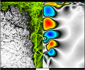
The instantaneous flow structures are discussed in this section to illustrate the shear-layer instabilities and the acoustic waves in the feedback loop in the under-expanded supersonic impinging jets of this study. The contour plots of the density gradient with an adjustment of the colour map are used to demonstrate both the formation and development of the shear-layer instabilities and the acoustic waves. The feedback loop mechanism proposed by Powell (Reference Powell1988) and Henderson & Powell (Reference Henderson and Powell1993) involves both downstream-propagating hydrodynamic and upstream-propagating acoustic waves. The fluctuations associated with the hydrodynamic waves are many orders of magnitude stronger than those associated with the acoustic waves. Thus, to clearly elucidate both components, contour plots of the density gradient with an adjustment of the colour map (i.e. white to black colour is used for  $\log (|\boldsymbol {\nabla } \rho |)$ between
  $-1$ and 0.5, while the black to green colour is used for
  $\log (|\boldsymbol {\nabla } \rho |)$ between 0.5 and 1.0) are provided in figures 4 and 5 for cases with the nozzle-to-wall distance of
  $2d$ and
  $5d$, respectively.

Figure 4. Instantaneous contour plots of the density gradient with a time interval of 0.26 acoustic time units (solid circles show the tracked vortical structures, dashed red curves show the tracked acoustic wave and  $y$ is related to the radius by
  $-r < y < r$).

Figure 5. Instantaneous contour plots of the density gradient with a time interval of 1.3 acoustic time units (dashed curves show the acoustic waves and  $y$ is related to the radius by
  $-r < y < r$).
We start with the nozzle-to-wall distance of  $2d$. Figure 4 shows the contour map of the instantaneous density-gradient field for this case. The contour maps are sequential snapshots with an equal time difference of 0.26 acoustic time units. This time is equivalent to 0.28 characteristic time of the jet based on inlet velocity and the nozzle diameter, and 0.34 characteristic time of the dominant coherent structures convected in the shear layer of this nozzle-to-wall distance considering these dominant structures travel by a speed which is approximately 0.7 jet exit velocity (0.77
 $a_o$) (see figure 7a). Both flow instabilities propagating downstream in the shear layer of the jet and acoustic waves propagating upstream in the medium are visible. Starting with the flow instability, a disturbance with a small wavelength grows as it convects in the shear layer. The disturbance has a wavelength of a nozzle radius as it convects one jet diameter downstream of the nozzle.
Evolution of one of these coherent structures in the shear layer is now discussed in more detail. This vortical structure grows as it convects in the first three-time instants from  $t_0$ to
  $t_2$. At
  $t_3$, it interacts with the oblique shock and pushes the oblique shock downstream. This interaction results in a deformation of this vortical structure. It reaches the stand-off shock at the next instant, and finally, it impinges on the wall and travels parallel to the wall in the wall jet. Here, the coherent structure is stretched in the radial direction and is compressed in the axial direction as it propagates in the wall jet. The impingement of this vortical structure and formation of an acoustic wave at the impingement region is visible at the time instant
  $t_6$.
The pattern of the acoustic wave indicates that it radiates cylindrically in this plane. The origin of the acoustic source can be estimated simply by tracing it back to the origin (Weightman et al. Reference Weightman, Amili, Honnery, Soria and Edgington-Mitchell2017b), which is found to be located near the impingement wall at  $0.8d$ from the jet centreline at this nozzle-to-wall distance. The concurrency of the impingement of a coherent structure on the wall and the appearance of an acoustic wave near the impingement wall suggests that there is a connection between these two processes.
Now, we turn our attention to the acoustic wave. The acoustic wave is formed near the impingement wall as just described, and it propagates towards the nozzle lip as shown in the four instants from  $t_0$ to
  $t_3$, where the blue arrow in figure 4(b) indicates the wave's propagation direction. It is reflected from the wall at the next instant,
  $t_3$, and travels as a wavefront as can be seen at instances
  $t_4$ and
  $t_5$. The acoustic wave comes in from the front and perpendicular to the flow direction, which is consistent with the observation in the recent experimental study of Weightman et al. (Reference Weightman, Amili, Honnery, Edgington-Mitchell and Soria2019). The propagation of the acoustic waves along the wall after reflecting from the wall was also demonstrated using the linear impulse response in our recent study of the receptivity process in the same configuration as this study (Karami et al. Reference Karami, Stegeman, Ooi, Theofilis and Soria2020). The acoustic wave reaches the nozzle lip, and a shear-layer instability is initialised, and, hence, the feedback loop is completed.
The acoustic waves generated in the impingement region are considered the strongest compared to the other possible acoustic sources based on the strength of the density gradient. Acoustic waves are also created by interactions of large coherent structures with the oblique shock and the stand-off shock. However, these acoustic waves are weaker than the acoustic waves generated by the impingement of the coherent structures on the wall. As can be seen in figure 4, the density gradient is intense for the acoustic wave formed by the impingement of a coherent structure on the wall compared to the acoustic waves created by interactions of large coherent structures with the oblique shock and the stand-off shock.
Turning our attention to the case with the nozzle-to-wall distance of  $5d$, contour plots of the instantaneous density gradient for this nozzle-to-wall distance are presented in figure 5 for four instants with a time interval of 1.3 acoustic time units. (This time is equivalent to 1.68 characteristic time of the dominant coherent structures travel in the shear layer of this nozzle-to-wall distance considering these dominant structures propagate with a speed which is approximately 0.7 jet exit velocity (0.77
 $a_o$) (see figure 9a).) At first instant,
  $t_0$, two acoustic waves are visible. The wavefronts of these two acoustic waves are marked with the red and blue dashed curves while the propagation directions are shown by arrows. These waves radiate from the same region, i.e. the impingement region. At this instant, a strong interaction of a large coherent structure and an oblique shock is also visible (marked with a solid circle). The oblique shock is pushed downstream by this coherent structure and, consequently, this coherent structure is deformed. This leads to the creation of an acoustic wave outside of the shear layer (marked with a solid red curve at this instant) similar to the experimental results observed by Edgington-Mitchell et al. (Reference Edgington-Mitchell, Weightman, Honnery and Soria2018b). At the next instant,
  $t_1$, the acoustic wave, created at the impingement region, propagates almost half of the nozzle-to-wall distance. It propagates towards the wall and is reflected from the wall. The acoustic wave is internalised, and a shear-layer instability is formed via the receptivity at
  $t_3$.
Similar to the other nozzle-to-wall distance, the acoustic wave radiates cylindrically in this plane and the origin of the acoustic source can be estimated to be located at  $1.1d$ from the jet centreline at this nozzle-to-wall distance. In the numerical study of an under-expanded jet with NPR of 4.03 impinging on a flat surface (Gojon et al. Reference Gojon, Bogey and Marsden2015) (similar to the configuration of this study but with higher NPR and thin nozzle lip), two acoustic sources with different origins are found where the one contributes to close the feedback loop found to be located in the shear layer at the impingement wall, similar to the observation in the present study. However, in the recent experimental study of an under-expanded jet with NPR of 3.4 impinging on a cylindrical surface with a nozzle-to-wall distance of
  $3.5d$ by Weightman et al. (Reference Weightman, Amili, Honnery, Soria and Edgington-Mitchell2017b), it was found that the origin of the acoustic source which contributes to close the feedback loop is located near the impingement wall and at
  $1.4d$ from the jet centreline.
To visualise the vortex pairing and rolling process, the contour plots of instantaneous vorticity magnitude for the case with the nozzle-to-wall distance of  $5d$ are presented in figures 6(a)–6(d). (The vorticity near the nozzle of the other case shows the same behaviour and, hence, is not presented for the sake of brevity.) The sequences are selected to show both processes of vortex rolling/pairing and rolling/without pairing. The solid blue arrow shows the direction of a rolling/pairing process. Two vortices come together, roll and pair, and form a larger coherent structure which is highly distorted due to the interaction with the oblique shock. These coherent structures propagate with a constant dominant group velocity. As can be seen in figures 6(a)–6(d), at most one or occasionally two pairings may occur which reduce the frequency by a factor of two or four, which is also reported by Ho & Nosseir (Reference Ho and Nosseir1981) and Le et al. (Reference Le, Johnstone, Kosasih and Renshaw2020). The black dashed line, in figures 6(a)–6(d), shows the direction of rolling/without pairing of a vortex as it travels downstream. The vortex size has significantly increased due to spatial growth and has a wavelength of the nozzle radius as it convects one jet diameter downstream of the nozzle, which is similar to experimental results of Brown & Roshko (Reference Brown and Roshko1974). The spatial growth of small-amplitude perturbations, as will be shown in § 3.4.2, is also the dominant process in the configuration of this study.

Figure 6. (a–d) Snapshots in the ( $x, r$) plane of vorticity downstream of the nozzle exit with a time interval of 0.26 acoustic time units (blue solid arrow shows a rolling/pairing process and the black dashed arrow shows the rolling/without pairing event).
3.2. Flow structures and their characteristics
3.2.1. Temporal evolution
Using the time history of different quantities sampled at the shear layer and a straight vertical line at  $r = 2.0$, the characteristics of the flow structures are investigated quantitatively. Starting with the nozzle-to-wall distance of
  $2d$ case, figure 7(a) shows the streamwise velocity fluctuations along the shear layer, where the shear layer is approximated to be at the radial location of the maximum ensemble-averaged turbulent kinetic energy at each axial location. A periodic series of peaks and troughs is evident, which forms an organised pattern of wavepackets propagating downstream. The propagation velocity of the dominant wavepackets in the shear layer,
  $V_{s}$, is 0.77
 $a_o$. (The non-dimensionalised choked velocity at the exit of the nozzle (
 $V_e/a_o$) is 0.912 and the non-dimensionalised ideally expanded velocity (
 $U_j$) for NPR of 3.4 is 1.45
 $a_j$ (
 $a_j$ is the sound velocity at the ideally expanded condition); hence, the ratio of
  $U_j$ to
  $V_e$ is 1.33.) The propagation velocity is estimated by following a peak or a valley (i.e. a statistical estimation based on the slope of the velocity crest), as shown by a dashed red line in figure 7(a). The complex pattern observed in figure 7(a) indicates the different time scales of the flow features in the shear layer of the jet which is consistent with the previous study of an ideally expanded supersonic jet impinging on an inclined plate (Brehm, Housman & Kiris Reference Brehm, Housman and Kiris2016). Figure 7(b) shows the time history of the pressure fluctuations on a vertical straight line at
  $r = 2.0$. There are two patterns; one represents waves travelling from the impingement wall towards the nozzle, and the other waves travelling from the infinite-lipped nozzle towards the impingement wall. Both waves are propagating with the speed of sound, which confirms the acoustic nature of these waves. In contrast to space–time plots of the velocity fluctuations, the pattern is less perturbed with limited flow features. This is expected in the region away from the periphery of the jet where the flow is irrotational and acoustic waves are dominant.

Figure 7. Time history of (a) streamwise velocity fluctuations along the shear layer of the jet and (b) pressure fluctuations on a straight streamwise line at  $r = 2.0$ for the nozzle-to-wall distance of
  $2d$.
$2d$.
The characteristics of the wavepackets can be examined further using a spatio-temporal decomposition of the time history of the velocity and pressure at the shear layer and pressure at the near field. Figure 8 shows the frequency-wavenumber ( $St-k_x$) spectra of (a) streamwise velocity fluctuations extracted at the shear layer, (b) pressure fluctuations extracted at the shear layer, and (c) pressure fluctuations extracted at
  $r = 2.0$ and
  $0.0 < x < 1.5$ of the under-expanded supersonic impinging jet with the nozzle-to-wall distance of
  $2d$. The dominant downstream-travelling waves in the shear layer of the jet have a positive propagation velocity as expected. The propagation velocity of these wavepackets is 0.77
 $a_o$, which is similar to the findings in the time history of the velocity fluctuations (figure 7a). Figure 8(b) shows frequency-wavenumber (
 $St-k_x$) spectra of pressure fluctuations extracted at the shear layer. There are low-frequency waves which have negative propagation velocities indicating upstream-travelling waves in the shear layer of the jet. (It is noted that the phase velocity of each wave defined as
  $\omega / k (St/(k_x/2{\rm \pi} ))$ and the group velocity is defined as
  ${\partial \omega }/{\partial k}$ and is therefore proportional to the slope of the dispersion relation, and it is the propagation velocity of the dominant waves.) The existence of these waves have been reported in previous studies of supersonic jets (Bogey & Gojon Reference Bogey and Gojon2017; Edgington-Mitchell et al. Reference Edgington-Mitchell, Jaunet, Jordan, Towne, Soria and Honnery2018a) and subsonic jets (Towne et al. Reference Towne, Cavalieri, Jordan, Colonius, Schmidt, Jaunet and Brès2017). The dispersion relation for the pressure fluctuations extracted at
  $r = 2.0$ and
  $0.0 < x < 1.5$ is presented in figure 8(c). There are both upstream- and downstream-travelling waves with a propagation velocity equal to the speed of sound. It appears that the upstream-travelling waves are stronger. The strong near-field downstream-travelling waves are due to the configuration of this study which is an infinite-lipped nozzle. The frequency-wavenumber spectrum of pressure shows a wide range of wavelengths in the vicinity of the dominant frequency (i.e.
  $St$ number), which is also reported in the finite-lipped ideally expanded supersonic impinging jets (Bogey & Gojon Reference Bogey and Gojon2017). These large wavelengths are associated with the sharp pressure gradient of acoustic waves at the wavefronts, and the sharp gradient is more conceivable in the instantaneous contour plots of the density gradient (marked with dashed red curves) in figures 4 and 5.

Figure 8. Frequency-wavenumber spectra of (a) streamwise velocity fluctuations extracted at the shear layer, (b) pressure fluctuations extracted at the shear layer, and (c) pressure fluctuations extracted at  $r = 2.0$ and
  $0.0 < x < 1.5$ of the impinging under-expanded supersonic jet with the nozzle-to-wall distance of
  $2d$.
$2d$.
Considering the case with the nozzle-to-wall distance of  $5d$, figure 9(a) shows the history of the streamwise velocity fluctuations at the shear layer of the jet. An organised pattern of wavepackets is formed before the first Mach disk; these wavepackets propagate with speed,
  $V_{s}$, which is approximately 0.77
 $a_o$. This pattern is distorted as wavepackets interact with the first oblique shock; however, the dominant feature, i.e. the high amplitude wave, travels with nearly constant velocity. The pattern in the time-space of the velocity fluctuations at the shear layer shows a wide range of flow features in this nozzle-to-wall distance compared to the case with the nozzle-to-wall distance of
  $2d$. Now turning our attention to the time history of the pressure fluctuations on a straight vertical line at
  $r = 2.0$, acoustic waves are propagating upstream and are reflected by the infinite-lipped nozzle. This observation is similar to the behaviour observed in figure 7(b) for the case
  $h=2d$.

Figure 9. Time history of (a) streamwise velocity fluctuations along the shear layer of the jet and (b) pressure fluctuations on a straight streamwise line at  $r = 2.0$ for the nozzle-to-wall distance of
  $5d$.
$5d$.
The dispersion relation for the streamwise velocity and pressure fluctuations at the shear layer and pressure fluctuations at  $r = 2.0$ are presented in figures 10(a), 10(b) and 10(c) for the case with the nozzle-to-wall distance of
  $5d$. Similar to the case with nozzle-to-wall distance of
  $2d$, the dominant downstream-travelling wave in the shear layer of the jet has a positive propagation velocity with a propagation velocity of 0.77
 $a_o$ (figure 10a). There are also wavepackets with a negative wavenumber (figure 10b) which indicates the presence of upstream-travelling waves in the shear layer of this nozzle-to-wall distance similar to the case with the nozzle-to-wall distance of
  $2d$, consistent with previous experimental (Edgington-Mitchell et al. Reference Edgington-Mitchell, Jaunet, Jordan, Towne, Soria and Honnery2018a) and numerical (Gojon et al. Reference Gojon, Bogey and Marsden2015) studies of under-expanded supersonic jets and numerical studies of subsonic jet (Towne et al. Reference Towne, Cavalieri, Jordan, Colonius, Schmidt, Jaunet and Brès2017). It is noted that these upstream propagation waves could be either free stream upstream-propagating acoustic waves (Weightman et al. Reference Weightman, Amili, Honnery, Edgington-Mitchell and Soria2019) or intrinsic upstream-propagating acoustic waves (Jaunet et al. Reference Jaunet, Mancinelli, Jordan, Towne, Edgington-Mitchell, Lehnasch and Girard2019) which overlap when the group velocity is negative and equal to the speed of sound. The dispersion relation for the pressure fluctuations extracted at
  $r = 2.0$ and
  $0.0 < x < 4.1$ (figure 10c) shows both upstream- and downstream-travelling wavepackets with propagation velocity equal to the speed of sound.

Figure 10. Frequency-wavenumber spectra of (a) streamwise velocity fluctuations extracted at the shear layer, (b) pressure fluctuations extracted at the shear layer, and (c) pressure fluctuations extracted at  $r = 2.0$ and
  $0.0 < x < 4.1$ of the impinging under-expanded supersonic jet with the nozzle-to-wall distance of
  $5d$.
$5d$.
3.2.2. Dominant time scale
In order to clarify the nature of the coherent structures in the under-expanded impinging jets with these two nozzle-to-wall distances, the autocorrelations of the streamwise and radial velocity fluctuations at the shear layer are presented in figures 11 and 12. Figure 11 shows the autocorrelations of (a) the streamwise and (b) the radial velocity fluctuations for sample points at the shear layer of the  $h=2d$ case. The autocorrelation of the streamwise velocity fluctuations (figure 11a) shows a large undershoot near to the peak, which indicates that the coherent structures are dominant in this flow (Brehm et al. Reference Brehm, Housman and Kiris2016). Figure 11(b) shows the autocorrelation of radial velocity fluctuations for the
  $h = 2d$ case. There are negative–positive alternations in the autocorrelation, which indicate the presence of a dominant coherent structure for this nozzle-to-wall distance with a time scale of approximately 1.1 acoustic time units. For the sake of clarity, the profiles of the autocorrelations of the radial velocity fluctuations at different axial locations are presented in appendix A, where the positive–negative alternations in the autocorrelation are clearer.

Figure 11. Autocorrelation of the (a) streamwise, and (b) radial velocity fluctuations for the sample points at the shear layer for the nozzle-to-wall distance of  $2d$.
$2d$.

Figure 12. Autocorrelation of the (a) streamwise and (b) radial velocity fluctuations for the sample points at the shear layer for the nozzle-to-wall distance of  $5d$.
$5d$.
Figure 12 shows the autocorrelations of the (a) streamwise and (b) radial velocity fluctuations for sample points at the shear layer for the  $h = 5d$ case. There is a large undershoot near to the peak in the autocorrelation of the streamwise velocity fluctuations, as shown in figure 12(a), which is consistent with the case with the nozzle-to-wall distance of
  $2d$. A negative–positive alternation in the autocorrelation of the radial velocity fluctuations is also evident in this nozzle-to-wall distance. However, the time scale of the dominant coherent structure is approximately 2.2 acoustic time units (also see appendix A, figure 21b). This time scale corresponds to
  $St=$0.45, where
  $St$ number is defined based on the ambient sound velocity and actual nozzle diameter (
 $fd/a_o$). In the recent experimental study by Weightman et al. (Reference Weightman, Amili, Honnery, Edgington-Mitchell and Soria2019), the acoustic spectrum obtained using a long period microphone measurement shows that the dominant tone frequency has
  $St_j=0.385$ for the infinite-lipped nozzle with a nozzle-to-wall distance of 5
 $d$ where the
  $St_j$ number is defined based on the ideally expanded supersonic jet diameter (
 $d_j$) and ideally expanded velocity (
 $U_j$). Utilising the same non-dimensionalisation as in the experiment, the
  $St_j$ number corresponding to the
  $St$ number of the dominant coherent structure obtained using autocorrelation is 0.39.
The horizontal dashed lines in figures 11 and 12 indicate the locations of the oblique shock/shear-layer interactions for these two nozzle-to-wall distances. There are variations in the level of the undershoot in the autocorrelations due to these interactions. These interactions were also observed to deform the vortical structures in the contour plots of the density gradient presented in figures 4 and 5.
The time scale of the turbulent structures can be obtained by further decomposing the fluctuations into a coherent part and a random fluctuation part. This approach, which is commonly known as triple decomposition (Hussain & Reynolds Reference Hussain and Reynolds1970), was used recently by Zhang & Wu (Reference Zhang and Wu2020) to study acoustic radiation of coherent structures in subsonic turbulent free shear layers and previously by Edgington-Mitchell et al. (Reference Edgington-Mitchell, Oberleithner, Honnery and Soria2014b) to study the coherent structures in free under-expanded supersonic jets. The autocorrelation of random fluctuations of the radial velocity (i.e.  $u''_r$) at the shear layer are presented in figures 13(a) and 13(b) for the
  $h = 2d$ and
  $5d$ cases, respectively. The random fluctuations are calculated by subtracting the coherent part of the fluctuations from the total fluctuations, where the coherent part is obtained by bandpass filter of the velocity fluctuations around the dominant frequency (i.e.
  $St$ of 0.91 for the
  $h = 2d$ case and
  $St$ of 0.45 for the
  $h = 5d$ case) with lower and upper bands being 5 % of the dominant frequency. The integral time scales of these random fluctuations, which are obtained by integrating the autocorrelation functions, are presented for both cases in figure 13(c). These random structures have time scales of an order of magnitude smaller than the time scale of the dominant coherent structures in both cases. This separation in time scales indicates that the random fluctuations have no significant contribution to the coherent dynamics embedded in this flow configuration. This also indicates that the linear stability analysis is valid to study the coherent structures in this configuration (Oberleithner, Rukes & Soria Reference Oberleithner, Rukes and Soria2014).

Figure 13. Autocorrelation of the radial velocity random fluctuations for sample points in the shear layer for the nozzle-to-wall distance of (a)  $2d$, (b)
  $5d$ and (c) integral temporal scales along the shear layer of both cases of the nozzle-to-wall distance of
  $2d$ and
  $5d$.
$5d$.
3.3. Acoustic-hydrodynamic coupling (non-normalised cross-correlation)
In § 3.2.1 we demonstrated that the dominant instabilities at the shear layer of both jets propagate downstream with a nearly same propagation velocity of 0.77 $a_o$ and acoustic wavepackets travel with the speed of sound in the near field of the nozzle. Autocorrelation of the velocity fluctuations in the shear layer is used to show that these structures have a dominant time scale of 1.1 and 2.2 acoustic time units for the
  $h = 2d$ and
  $5d$ cases, respectively. Tam (Reference Tam1986) proposed that excitation of the intrinsic instability waves in shear flows requires two conditions. The frequencies of the incident sound wave and the excited instability wave should be matched as well as the phase velocities of the two waves. The matching of the frequency for the two signals to interact is expected; however, the second condition is not easy to conceive. Ho & Nosseir (Reference Ho and Nosseir1981) showed that a phase lock at resonance frequency is essential for the coupling of acoustic and hydrodynamic waves at the nozzle lip which does not dictate the phase velocity matching condition of Tam (Reference Tam1986). From the dispersion relation, it is clear that the second condition proposed by Tam (Reference Tam1986) is not satisfied in the configuration of this study and the dominant acoustic and instability waves have two different propagation velocities with opposite sign (i.e. propagating in the opposite direction) similar to previous experimental studies of high-speed flows by Nosseir & Ho (Reference Nosseir and Ho1979) and Ho & Nosseir (Reference Ho and Nosseir1981). However, both acoustic wavepackets in the near field and shear-layer instabilities should have a different wavelength to maintain the same frequency. To demonstrate the length scale of these two waves, the spatial cross-correlation of the near-field pressure fluctuations at
  $x = 1.0$ and
  $r = 2.0$ with pressure fluctuations and velocity fluctuations are presented in this section. The non-normalised cross-correlation of a variable
  $\phi$ at a fixed location of
  $(x_{ref}, r_{ref})$ in the
  $x$–
$x$– $r$ plane and a variable
  $\chi$ is defined as
 \begin{equation} C_{\phi \chi} = \frac{1}{N_t \times N_{\theta}} \sum_{i=1}^{N_t}\sum_{j=1}^{N_{\theta}}\phi(x_{ref},r_{ref},\theta_j , t_i) \chi(x,r,\theta_j , t_i), \end{equation}
where  $N_t$ is the number of snapshots over which the average is computed and
  $N_{\theta }$ is the number of azimuthal grids. The non-normalised cross-correlation is utilised to reveal coherent structures. In the recent study of noise generation in a supersonic jet impinging on an inclined plate by Brehm et al. (Reference Brehm, Housman and Kiris2016), both non-normalised and normalised cross-correlations were utilised to identify the acoustic source location. It was found that the non-normalised cross-correlation is a better measure to determine the acoustic source location as it retains information about the amplitudes of fluctuations in the source region. On the other hand, the normalised cross-correlation gives high weight to the events which are not statistically significant and have small variance at near-field regions and could not reveal the acoustic source location. In the configuration of under-expanded supersonic jets of this study, it was found that both normalised and non-normalised cross-correlations can be employed to reveal the dominant coherent structures; however, the acoustic waves are clearer in the non-normalised cross-correlation. For the sake of brevity, the non-normalised cross-correlation is discussed in this section, while the normalised cross-correlation is presented in appendix B.
For the configurations of this study, which contains a single significant periodic time component, the spatial distribution of the cross-correlation maps reveals the large-scale behaviour (Bell et al. Reference Bell, Soria, Honnery and Edgington-Mitchell2018). The contour map of non-normalised cross-correlation for the reference pressure fluctuations at  $x = 1.0$ and
  $r = 2.0$ and the pressure (
 $C_{p'p'}$) is presented in figure 14(a), while figure 14(b) presents the contour map of non-normalised cross-correlation for the reference pressure fluctuations at
  $x = 1.0$ and
  $r = 2.0$ and the radial velocity (
 $C_{p'u'_{r}}$) for the nozzle-to-wall distance of
  $2d$. The non-normalised cross-correlation of the pressure fluctuation shows clear correlations between the near-field pressure fluctuations and both oblique and stand-off shocks, which indicate the oscillations of the stand-off and oblique shocks coupled with the creation of acoustic waves for this nozzle-to-wall distance. This is also conceivable in the normalised cross-correlation presented in figure 22(a) in appendix B. The acoustic wave has a wavelength,
  $\lambda _a$, of approximately
  $1d$. Figure 14(b) shows the non-normalised cross-correlation for the observation reference of the pressure fluctuations at
  $x = 1.0$ and
  $r = 2.0$ and the radial velocity,
  $C_{p'u'_{r}}$. There is a strong correlation of the radial velocity fluctuations and near-field reference pressure at locations of the oblique shock, stand-off shock, wall jet and shear layer of the jet which is clearer in the normalised cross-correlation presented in figure 22(b) in appendix B. The dominant downstream-travelling wave in the shear layer has a wavelength,
  $\lambda _s$, of approximately
  $0.85d$. Considering the propagation velocity and wavelength, it is trivial to find the frequency or the time scale,
  $\tau = \lambda / V$, of these wavepackets. The time scales of both acoustic waves and shear-layer instabilities are found to be 1.1 acoustic time unit which is consistent with the time scale obtained from the autocorrelation analysis presented in § 3.2.2.

Figure 14. The contour maps of non-normalised cross-correlation for the observation reference of the pressure fluctuations at  $x = 1.0$ and
  $r = 2.0$ and (a) pressure (
 $C_{p'p'}$), (b) radial velocity (
 $C_{p'u'_{r}}$) for the nozzle-to-wall distance of
  $2d$.
$2d$.
Figure 15 shows the same quantities as in figure 14 for the  $h = 5d$ case with an observation reference of the pressure fluctuations at
  $x = 2.5$ and
  $r = 4.25$. The pressure at the reference point is correlated with pressure modulations in the shear layer and the centre of the jet (see also figures 23a and 23b in appendix B). The acoustic wave has a wavelength,
  $\lambda _a$, of approximately
  $2d$ (figure 15a). The pressure at the reference point is strongly correlated with the shear-layer instabilities in contrast to the
  $h=2d$ case. The shear layer has a wavelength,
  $\lambda _s$, of approximately
  $1.7d$. These wavelengths with their corresponding propagation velocities result in a time scale of 2.2 acoustic time units for both wavepackets, which is also consistent with the time scale obtained using the autocorrelation analysis presented in § 3.2.2.

Figure 15. Colour contours of non-normalised cross-correlation for the observation reference of the pressure fluctuations at  $x = 2.5$ and
  $r =4.25$ and (a) pressure (
 $C_{p'p'}$), (b) radial velocity (
 $C_{p'u'_{r}}$) for the nozzle-to-wall distance of
  $5d$.
$5d$.
3.4. Frequency characteristics of instability wavepackets
The most striking result obtained by the non-normalised cross-correlation is that the dominant coherent structures are formed approximately  $1d$ downstream of the nozzle lip. To the best of our knowledge, there exist two mechanisms to explain the formation of coherent low-frequency structures in shear flows: the collective interactive mechanism proposed by Ho & Nosseir (Reference Ho and Nosseir1981) and pairing of small high-frequency structures observed by Winant & Browand (Reference Winant and Browand1974) in a two-dimensional shear layer at moderately low Reynolds numbers. The former has only been reported in the study of a weakly under-expanded impinging jet by Diebold & Elliott (Reference Diebold and Elliott2014) and not been reported in previous studies of moderate and high under-expanded supersonic jets (Powell Reference Powell1953; Henderson & Powell Reference Henderson and Powell1993; Henderson, Bridges & Wernet Reference Henderson, Bridges and Wernet2005; Edgington-Mitchell et al. Reference Edgington-Mitchell, Honnery and Soria2014a) and have not been observed in this study, either. The pairing process requires a long distance to induce the reduction in the frequency of the initial instabilities, as also pointed out by Ho & Nosseir (Reference Ho and Nosseir1981). The other mechanism that might explain the formation of coherent low-frequency structures in a short distance of
  $1d$ is the exponential growth of instabilities. It is noted that the linear stability theory has been used widely to understand the underpinning physics in many flows (Hammond & Redekopp Reference Hammond and Redekopp1997; Pier Reference Pier2002; Barkley Reference Barkley2006; Sipp & Lebedev Reference Sipp and Lebedev2007; Mittal Reference Mittal2008; Oberleithner et al. Reference Oberleithner, Rukes and Soria2014; Sartor et al. Reference Sartor, Mettot, Bur and Sipp2015; Turton, Tuckerman & Barkley Reference Turton, Tuckerman and Barkley2015; Beneddine et al. Reference Beneddine, Sipp, Arnault, Dandois and Lesshafft2016; Illingworth, Monty & Marusic Reference Illingworth, Monty and Marusic2018); however, to-date, few studies have utilised this approach to reveal the fundamental physics behind instabilities in supersonic jets (Nichols & Lele Reference Nichols and Lele2011; Jaunet et al. Reference Jaunet, Mancinelli, Jordan, Towne, Edgington-Mitchell, Lehnasch and Girard2019) where the growth is being calculated on a varying base flow extracted from either experimental or numerical dataset. To the best of our knowledge, this study is the first to use this approach to study the frequency characteristics of the flow structures near the nozzle of under-expanded supersonic jets. Hence, the aim of this section is to investigate whether the linear instability growth can support the frequency reduction in a short distance of
  $1d$ in the configuration of under-expanded supersonic jets. This analysis then follows by spatial growth analysis based on the LES data to support the findings from the linearised analysis.
3.4.1. Linear spatial instability analysis
The ensemble-averaged streamwise velocity, pressure and density obtained from LES are substituted into (2.5) at each axial location to perform the spatial instability analysis. Before the discussion of the results obtained from this analysis, it is noted that the linear spatial instability analysis is used to evaluate the changes in the most unstable frequency as we progress downstream and not the growth rate. The base flow is obtained from LES and the mean profiles at each axial locations are used to perform local linear stability analysis.
Figures 16(a) and 16(b) show the ensemble-averaged streamwise velocity at the axial locations where the spatial instability analysis was performed. The profiles in both cases are very different from a tanh function which was used in previous studies for subsonic jets (Koshigoe et al. Reference Koshigoe, Gutmark, Schadow and Tubis1988; Gudmundsson & Colonius Reference Gudmundsson and Colonius2007; Gudmundsson Reference Gudmundsson2010; Lajús et al. Reference Lajús, Sinha, Cavalieri, Deschamps and Colonius2019). As can be seen in this figure, an increase in the nozzle-to-wall distance results in shifts in the inflection points of the mean profiles and, hence, different instability characteristics are expected. The shear layer of the case with the nozzle-to-wall distance of 2 $d$ seems to be slightly thicker. The spatial instability analysis is limited to the region between the nozzle lip and one jet diameter downstream of the nozzle lip as previous studies show that the instabilities in the potential core of the jet are dominated by modal instabilities and the non-modal behaviour kicks in far downstream of the potential core (Tissot et al. Reference Tissot, Zhang, Lajús, Cavalieri and Jordan2017; Lajús et al. Reference Lajús, Sinha, Cavalieri, Deschamps and Colonius2019). We also restrict our attention to the axisymmetric mode as it is found to be the leading dominant mode (see appendix C for further discussion) in the previous study of an under-expanded supersonic impinging jet with the same NPR and nozzle-to-wall distance (Weightman et al. Reference Weightman, Amili, Honnery, Edgington-Mitchell and Soria2019).

Figure 16. Profiles of ensemble-averaged streamwise velocity at different axial locations for the cases with a nozzle-to-wall distance of (a)  $2d$ and (b)
  $5d$.
$5d$.
The growth rates are presented in figure 17. Near to the nozzle at  $x = 0.1$, the growth rate is high with a broad range of unstable Strouhal numbers for both cases; however, the shear layer of the
  $h=2d$ case has a slightly wider range of unstable Strouhal numbers with the slightly lower maximum growth rate. The maximum growth rate rapidly reduces at axial stations further downstream. The upper band of the unstable Strouhal numbers also reduces at axial stations further downstream, and it is below
  $St$ of 1.2 at
  $x = 0.9$ for both cases. However, the Strouhal number with the maximum growth rate for both cases approaches a Strouhal number of 0.4, as shown in figure 18. This figure also shows that the
  $St$ number of the maximum growth rate of both cases converges to the same value as we progress downstream. This sharp decrease of the most unstable frequency shows that the shear layers of the under-expanded supersonic jets of this study support the formation of coherent low-frequency structures in a short distance from the nozzle lip.

Figure 17. The spatial growth rates obtained from solution of compressible Rayleigh equation at different axial locations for the cases with a nozzle-to-wall distance of (a)  $2d$ and (b)
  $5d$.
$5d$.

Figure 18. Strouhal number of the maximum growth rate as a function of axial location for both cases with the nozzle-to-wall distance of  $2d$ and
  $5d$.
$5d$.
3.4.2. Nonlinear spatial growth from LES
This section connects the findings based on parallel linear spatial instability analysis to the LES results, mostly discussing the evolution of the frequency band as the disturbances grow in the shear layer and not the growth rate itself. The evolution of disturbances in incompressible flows is characterised by the kinetic energy of the disturbances, which is commonly used to define the norm for the energy of disturbances. However, in compressible flows fluctuations of thermodynamic quantities contribute to the energy and need to be included (Mack Reference Mack1984; Hanifi, Schmid & Henningson Reference Hanifi, Schmid and Henningson1996; Freund & Colonius Reference Freund and Colonius2002; Tumin & Reshotko Reference Tumin and Reshotko2003; Ray, Cheung & Lele Reference Ray, Cheung and Lele2009; Paredes et al. Reference Paredes, Gosse, Theofilis and Kimmel2016); hence, the energy of the disturbances also known as the Mach energy norm is defined as
 \begin{equation} E = \frac{1}{2} \left( \bar{\rho} u'_i{u'_i}^{*} + \frac{\bar{T}\rho'{\rho'}^{*} }{\bar{\rho}\gamma M^2} + \frac{\bar{\rho}T' {T'}^{*} }{\gamma (\gamma-1)\bar{T}M^2}\right), \end{equation}
where  $*$ denotes the complex conjugate and
  $M$ is the Mach number, defined based on inlet velocity and the speed of sound based on inlet temperature. The fluctuation terms in (3.2) are obtained by decomposing the three-dimensional disturbance fields in the azimuthal direction, which is periodic, to limit the analysis to each azimuthal mode number. The azimuthally decomposed variables are used to obtain the energy of the disturbances using (3.2). The energy of the disturbances is then temporally decomposed using temporal Fourier transform to investigate their frequency characteristics. To obtain the norm of the energy, integration of the energy in an appropriate domain is required. In order to characterise the spatial development of the disturbances in the shear layer, the integration is performed in the radial direction to obtain an appropriate measure for streamwise growth of the disturbances. In contrast to previous studies of jet and shear flows (Oberleithner et al. Reference Oberleithner, Rukes and Soria2014; Lesshafft et al. Reference Lesshafft, Semeraro, Jaunet, Cavalieri and Jordan2019), where the lower and upper limits of the integration are centreline and infinity, the upper and lower limits are confined to obtain an accurate measure of shear-layer instabilities as in the present configuration a Mach disk and an oblique shock also play a role, and, hence, the norm of the energy of disturbances is defined as
 \begin{equation} A (x,m,St)= \int_{r_{l}}^{r_{u}} \hat{E}(x,r,m,St)r \,\textrm{d}r, \end{equation}
where  $\hat {.}$ denotes Fourier transform of
  $E$,
$E$,  $r_{l}$ and
  $r_{u}$ are the upper and lower limits of the integration, respectively. These limits are defined as the radial locations of the maximum velocity gradient on two sides of the shear layer. These definitions are demonstrated in figure 19. The contour map presents the energy of disturbances for the axisymmetric mode and
  $St = 1.2$ (the colourmap is normalised between 0 and 1 for the purpose of demonstration), where the lower and upper limits of the integration in (3.3) are presented by red and black dots, respectively.

Figure 19. The energy of disturbances for the axisymmetric mode and  $St$ of 1.2 (the colour map is normalised between 0 and 1 for the purpose of demonstration). The lower and upper limits of the integration in (3.2) are presented by red and black dots, respectively.
The contour plot of the norm of the energy,  $A$, for both nozzle-to-wall distances of
  $2d$ and
  $5d$ are presented in figures 20(a) and 20(b), respectively. It is clear from the figure that the high-frequency disturbances are saturated by strong low-frequency disturbances as they travel in the shear layer by only 1
 $d$. The red circles are the Strouhal number of the maximum growth rate at each axial station obtained from linear spatial instability analysis (see figure 18). It appears linear instability analysis underpredicts the most unstable frequency (Strouhal number); however, the trend of decreasing the unstable Strouhal number is well predicted. This discrepancy is associated with the parallel flow assumptions in the linear stability analysis. In the under-expanded supersonic jet, the parallel flow assumption is not valid, and the mean profiles (streamwise velocity shown while density, pressure, radial velocity profiles are also a function of radial location) vary drastically in the axial direction as shown for the axial velocity profiles in figure 16. It is also noted that the linear parabolised stability equations (PSE), where the assumption of parallel flow is relaxed, is expected to deliver a better agreement with LES results (Sinha et al. Reference Sinha, Gudmundsson, Xia and Colonius2016; Kim et al. Reference Kim, Lim, Kim, Jee, Park and Park2019; Towne, Rigas & Colonius Reference Towne, Rigas and Colonius2019; Wong et al. Reference Wong, Edgington-Mitchell, Honnery, Cavalieri and Jordan2019).

Figure 20. The norm of energy,  $A$, of the axisymmetric mode (
 $m=0$) for the cases with the nozzle-to-wall distance of (a)
  $2d$ and (b)
  $5d$. (The red circles are the Strouhal number of the maximum growth rate obtained from linear spatial instability analysis.)
4. Conclusion
Two main ingredients of the feedback loop in the under-expanded supersonic impinging jets, the hydrodynamic instabilities in the shear layer and acoustic waves in the medium, have been illustrated utilising the instantaneous time evolution of the density gradient from LES in the streamwise-radial plane. The spatial histories of the streamwise velocity fluctuations along the shear layer of the jets show that hydrodynamic instabilities are dominantly convected downstream with the propagation velocity of 0.77 ambient speed of sound (0.7 jet exit velocity) for both cases. The near-field acoustic waves travel in both upstream and downstream directions with the speed of sound as expected for both nozzle-to-wall distances. The propagation velocities of both acoustic and instability wavepackets were obtained using a dispersion relation analysis and are in agreement with the spatial history analysis.
The autocorrelations of the velocity fluctuations show that the flows exhibit a single significant periodic time scale, which is 1.1 and 2.2 acoustic time units for the nozzle-to-wall distances of  $2d$ and
  $5d$, respectively. The autocorrelations of the triple decomposed velocity fluctuations show that the small-scale turbulent structures, which have a random nature, have no influence on the dominant coherent structures in these flows. Cross-correlation analysis was employed to reveal the acoustic and instability wavelengths corresponding to this single time scale. The cross-correlation analysis also reveals that these dominant coherent structures are generated approximately one jet diameter downstream of the nozzle lip.
The mechanism by which the initial high-frequency instability changes to a low-frequency coherent structure in a short distance of approximately 1 $d$ is investigated. It is shown that the shear layer of under-expanded supersonic jets in contrast to their subsonic counterparts support the changes in the most unstable frequency of the instabilities in the very short distance of 1
 $d$, which its trend is reasonably well predicted by linear spatial instability analysis where the mean profiles of the primitive variables (i.e. velocity components, density and pressure) are considered to vary in the streamwise direction. This strong dependence on the local mean shear-layer profile suggests a need for care when using vortex sheet or tanh approximations (i.e. the parallel flow assumption with streamwise uniform mean shear-layer velocity) to calculate growth rates and the most unstable frequencies.
Acknowledgements
This work was supported by the Australian Research Council. The research benefited from computational resources provided through the National Computational Merit Allocation Scheme, supported by the Australian Government. The computational facilities supporting this project included the Australian NCI Facility, the partner share of the NCI facility provided by Monash University through a ARC LIEF grant, Pawsey Supercomputing Centre and the Multi-modal Australian ScienceS Imaging and Visualisation Environment (MASSIVE).
Declaration of interests
The authors report no conflict of interest.
Appendix A. Profiles of autocorrelation and dominant time scale
Figure 21(a) shows the profiles of the autocorrelation of the radial velocity fluctuations at the shear layer (the contour map is presented in figure 11b) extracted at axial locations between 0.8 and 1.3 with an increment of 0.1 for the case with the nozzle-to-wall distance of  $2d$, while figure 21(b) shows the profiles of the same quantity (the contour map is presented in figure 12b) extracted at axial locations between 1.5 and 2.5 with an increment of 0.1 for the case with the nozzle-to-wall distance of
  $5d$. The negative–positive alternation in the autocorrelations are more conceivable in these figures as well as the time scale of the dominant coherent structure which were found to be approximately 1.1 and 2.2 acoustic time units for the cases with the nozzle-to-wall distance of
  $2d$ and
  $5d$, respectively.

Figure 21. Profiles of autocorrelation of the radial velocity fluctuations for the sample points at the shear layer (a)  $h = 2d$ (profiles are for axial locations
  $0.8 < x < 1.3$ with an increment of 0.1), (b)
  $h = 5d$ (profiles are for axial locations
  $1.5 < x < 2.5$ with an increment of 0.1).
Appendix B. Normalised cross-correlation
The normalised cross-correlation of a variable  $\phi$ at a fixed location of
  $(x_{ref}, r_{ref})$ in the
  $x-r$ plane and a variable
  $\chi$ is defined as
 \begin{align} &\langle C_{\phi \chi}\rangle = \frac{C_{\phi \chi}}{C_{\phi} C_{\chi}} \nonumber\\ &\quad = \frac{ \dfrac{1}{N_t \!\times\! N_{\theta}}\sum_{i=1}^{N_t}\sum_{j=1}^{N_{\theta}} \phi(x_{ref},r_{ref},\theta_j , t_i) \chi(x,r,\theta_j , t_i)}{\left(\dfrac{1}{N_t \!\times\! N_{\theta}}\sum_{i=1}^{N_t}\sum_{j=1}^{N_{\theta}}\phi^2(x_{ref},r_{ref},\theta_j , t_i)\right)^{{1}/{2}} \left(\dfrac{1}{N_t \!\times\! N_{\theta}} \sum_{i=1}^{N_t}\sum_{j=1}^{N_{\theta}} \chi^2(x,r,\theta_j , t_i)\right)^{{1}/{2}}}, \end{align}
where  $N_t$ is the number of snapshots over which the average is computed and
  $N_{\theta }$ is the number of azimuthal grids.
Figures 22(a) and 22(b) show the contour map of normalised cross-correlation for the reference pressure fluctuations at  $x = 1.0$ and
  $r = 2.0$ and the pressure (
 $\langle C_{p'p'}\rangle$) and the radial velocity (
 $\langle C_{p'u'_{r}}\rangle$) for the nozzle-to-wall distance of
  $2d$. The correlations between the near-field pressure fluctuations and both oblique and stand-off shocks is clearer in these subfigures which indicate the oscillations of the stand-off and oblique shocks are coupled with the creation of acoustic waves for this nozzle-to-wall distance. Figure 23 shows the same quantities as in figure 22 for the case with a nozzle-to-wall distance of
  $5d$ with an observation reference of the pressure fluctuations at
  $x = 2.5$ and
  $r = 4.25$. The correlation of the pressure at the reference point and pressure modulations in the shear layer and the centre of the jet is more conceivable in figure 23(a) and the correlation of the pressure at the reference point with the shear-layer instabilities (figure 23b) in contrast to the
  $h=2d$ case is strong.

Figure 22. The contour maps of normalised cross-correlation for the observation reference of the pressure fluctuations at  $x = 1.0$ and
  $r = 2.0$ and (a) pressure (
 $\langle C_{p'p'}\rangle$), (b) radial velocity (
 $\langle C_{p'u'_{r}}\rangle$) for the nozzle-to-wall distance of
  $2d$.
$2d$.

Figure 23. Colour contours of normalised cross-correlation for the observation reference of the pressure fluctuations at  $x = 2.5$ and
  $r =4.25$ and (a) pressure (
 $\langle C_{p'p'}\rangle$), (b) radial velocity (
 $\langle C_{p'u'_{r}}\rangle$) for the nozzle-to-wall distance of
  $5d$.
$5d$.
Appendix C. Energy norm of azimuthal modes
In § 3.4 we restricted our attention to the axisymmetric mode, to elaborate on this choice the norm of the energy of disturbances defined in (3.3) is integrated in both the axial and frequency domain to obtain the norm of the energy associated with each azimuthal mode number as
 \begin{equation} \bar{A} (m)= \int_{0}^{St = 8.0} \int_{0}^{x_{o}} A (x,m,St) \,\textrm{d}St \,\textrm{d}x, \end{equation}
where  $x_o$ is the maximum
  $x$ location confined by red and black dashed lines in figure 19 (i.e. the spatial area of the integration is the region confined by red and black dashed lines in figure 19). Using this equation, the energy of disturbances of each azimuthal mode is accessed utilising the normalisation defined as
 \begin{equation} \varUpsilon (m)= \frac{\bar{A} (m)}{\sum_{m=0}^{9}\bar{A} (m)} \times 100. \end{equation}
Figure 24 shows the normalised energy of disturbances as a function of the azimuthal mode number. It is clear from this figure that the axisymmetric mode is the dominant mode.

Figure 24. The normalised energy of disturbances as a function of azimuthal mode number for both cases,  $h=2d$ and
  $5d$.
$5d$.


