4.1. Connection to scaling laws

The measurement of the high m/q distribution appearing along small mass-to-charge species suggests that the operational mode at these flow rates is that of the mixed ion–droplet form. Several studies have demonstrated a link between total emission current and liquid parameters appropriate for the single cone-jet operating in a mixed ion–droplet mode (Fernández de la Mora & Loscertales Reference Fernández de la Mora and Loscertales1994; Gañán-Calvo Reference Gañán-Calvo1997; Gañán-Calvo et al. Reference Gañán-Calvo, Dávila and Barrero1997; Gamero-Castaño & Fernández de la Mora Reference Gamero-Castaño and Fernández de la Mora2000). Our attention here is on the recent work of Gañán-Calvo et al. that has demonstrated broad applicability, for both neat systems and solutions, of the predictive capability using dimensionless values (Gañán-Calvo et al. Reference Gañán-Calvo, López-Herrera, Herrada, Ramos and Montanero2018). Figure 8(a) presents the experimental current measurements (top) and predicted mean droplet diameter (bottom) converted into dimensionless values of I/I ₀ and D/D ₀ plotted against the dimensionless flow rate, Q/Q ₀. The theoretical values, numerically evaluated from a best fit of a large number of systems, are shown as the dashed line. The EMI-IM and BMI-IM current values have an average deviation of +13.5 % and −14.3 % from the theoretical prediction. Beyond the slight offset, the data points parallel the ideal behaviour with perhaps some deviation at the lowest flow rates measured. The average reproducibility of the reported current measurements had a standard deviation of <3 % for 12 separate flow rates. ‘Error bars’ on the EMI-IM data depict the maximum extent (95 % confidence) of values possible using two times the standard deviation of the values for the reported physical parameters used to populate table 1. The extended ranges show excellent overlap with the theoretical prediction. Taken as a whole, the data of the four ILs illustrate that the emission current scaling law well reproduces the experimental current at the selected volumetric flow rates and the experimental current is consistent with that of a single cone-jet structure operating in a mixed ion–droplet mode. The predicted D/D ₀ is shown for EMI-IM and BMI-IM as the other liquids also lie along the same line when plotted against Q/Q ₀ and are not included to reduce overlap. The strong data correspondence for D/D ₀ is the result of the similar physical property values of the ILs. The predicted D/D ₀ as compared with the droplet diameter derived from experimentally measured values will be discussed below. Under the assumption that the emission process involves only the mean droplet with the predicted diameter, the mean mass, m, of the droplet is easily determined using (4.1)

(4.1)\begin{equation}m = \rho (4/3{\rm \pi} R_{Drop}^3),\end{equation}

where ρ is the density and R_Drop is the radius of the droplet. The number of emitted droplets per second is then subsequently calculated so as to properly conserve mass. The measured emission current can then be distributed into mean charges per droplet and the average mass-to-charge value of the droplet readily determined. This value, which will agree with simply dividing the total mass flow by the total current flow, is shown in the top plot of figure 8(b) for three liquids, EMI-IM, BMI-IM and BMI-DCA, again as a function of the dimensionless flow rate. At the flow rates studied in this work, the expected primary droplets typically have significant charge values.

Figure 8. Comparison of the emitter output per dimensionless flow rate for the electrosprayed ILs BMI-IM, BMI-BF₄, EMI-IM and BMI-DCA using the dimensionless scaling laws of Gañán-Calvo et al. (Reference Gañán-Calvo, López-Herrera, Herrada, Ramos and Montanero2018); (a – top) dimensionless current output with the dashed line representing the theoretical prediction; (a – bottom) theoretical prediction of the dimensionless mean droplet diameter. The results overlap for each IL, thus only two are illustrated; (b – top) theoretical and experimental m/q values of the mean droplet shown for three ILs; (b – bottom) theoretical ratio of droplet mean charge to Rayleigh charge limit. The initial emitted mean droplets are expected to be super Rayleigh above Q/Q ₀ = 2147.

In the bottom of figure 8(b), the ratio of expected mean charge to the Rayleigh charge limit is shown as a function of dimensionless flow rate. The Rayleigh charge limit (q_ray) of a sphere is given as (4.2)

(4.2)\begin{equation}{q_{Ray}} = \; {[8{{\rm \pi} ^2}{\varepsilon _0}\gamma {(2{R_{Drop}})^3}]^{1/2}},\end{equation}

where γ is the surface tension and ε ₀ is the permittivity of free space. A dashed line in the figure divides the ratio at which the mean primary droplets are expected to be stable from those expected to be super-Rayleigh (>1). For all four liquids examined, the transition from sub- to super-Rayleigh occurs at a Q/Q ₀ value of 2147 as illustrated and is determined by evaluating q/q_Ray = 1 ≈ 0.147⋅(Q/Q ₀)^1/4. The data of BMI-DCA show the best agreement with this intersection point. Having established that previously determined scaling laws also apply in these experiments, we now turn our discussion to the experimentally determined jet velocities.

4.2. Determination of jet breakup quantities

The linear relationship between the offset DC potential and the high m/q droplet centroid value presented in figure 5 has been previously observed in studies of solutes dissolved in volatile solvents by Gamero-Castaño for a much larger droplet m/q value (Gamero-Castaño Reference Gamero-Castaño1999, Reference Gamero-Castaño2008a, Reference Gamero-Castaño2010; Gamero-Castaño & Hruby Reference Gamero-Castaño and Hruby2002). In those works, the kinetic energy, measured as the stopping distance required far downstream from the jet, was shown to describe the kinetic energy initially imparted by the jet and the energy gained as a result of the electric field in the acceleration zone. The resulting kinetic energy, E, of the emitted ions in this situation is

(4.3)\begin{equation}E = \frac{1}{2}mv_{Jet}^2 + q{\varPhi _{Tip}} \to \frac{E}{q} = \frac{1}{2}\left( {\frac{m}{q}} \right)v_{Jet}^2 + {\varPhi _{Tip}},\end{equation}

where v_Jet is the mean velocity of the jet at the point where the charged particles are released, m is the mass of the charged species, q is the charge of the species and Φ_Tip is the potential at which the jet breaks up and charged species are emitted. The kinetic energy per unit charge (E/q, right side of (4.3)) is readily determined by simple algebraic manipulation. In this altered form, the base DC potential applied to the two plates in the pulsing region is directly linked to the E/q value, within the ~25 eV q⁻¹ window described in the experimental section, while the mass spectrometer directly measures the m/q value of the ion. We again note that the base DC potential serves as a low-resolution stopping potential analyser of the emitted ion beam.

The high m/q droplet centroid data are presented as DC potential (E/q) vs. 1/2 m/q (all in SI units) in figure 9 for the IL BMI-IM at several selected flow rates. A linear modelling well fits the data at all flow rates. In accordance with (4.3), the slope and intercept values correspond to v_Jet and Φ_Tip. The square root of the slope is the jet velocity component and the intercept is directly the potential at the jet tip. For each BMI-IM electrospray flow rate probed, a mean jet velocity and jet breakup potential are now known. In addition to the high m/q droplet centroids, the potentials of the detected ions (i.e. n = 0–5) for some of the sampled flow rates are illustrated at the lowest m/q values. These BMI-IM ion data points are representative of the peak value of the ion data of EMI-IM illustrated in figure 6. Thus, the most intense population of ions align with the breakup potential of the high m/q droplets. As a result, at these flow rates, both the small ions and high m/q droplets appear to originate from the same location, namely, the end of the extended jet structure and not from the neck region of the Taylor cone.

Figure 9. BMI-IM data plotted for potential versus mass-to-charge ratio. The data points represent the high m/q droplet distribution centroids for select flow rates. Note the open symbols represent the singly charged ions n = 0–5 at each flow rate and correspond to the y-intercept potentials, Φ_Tip.

The coefficients v_Jet and Φ_Tip derived from the fits illustrated in figure 9 have been tabulated for all four ILs at select flow rates in table 3. The error values are at the 1-sigma confidence level (1σ). Φ_Ions is found by the best fit of a Gaussian distribution to the ion intensity vs. energy defect/potential data (i.e. the example ion distribution seen in figure 6). The lower uncertainties for the BMI-IM and BMI-BF₄ results reflect the finer energy defect probing used for those specific liquids. The EMI-IM data points with lower uncertainties also reflect a finer energy defect probing of 25 eV q⁻¹ intervals. For the set of flow rates and ILs measured, jet velocities ranging from 360 to 1000 m s⁻¹ are measured with typical uncertainties of approximately 10 % to 40 %. Of the studied ILs, BMI-DCA data provided the highest velocities, of the order 700 to 1000 m s⁻¹, which is nearly twice the velocity of EMI-IM and BMI-IM data points. The averaged jet velocities over the studied flow rates for BMI-DCA, EMI-IM, BMI-IM and BMI-BF₄ are 824 (±110), 528 (±61), 442 (±58) and 615 (±41) m s⁻¹ at the 1σ level uncertainty, respectively. In the case of cation versus anion performance, the limited BMI-IM anion results are consistent with the surrounding cation data within the uncertainties. Thus, we conclude similar jet velocities and breakup potentials are achieved no matter the charge polarity of the electrospray system. The measured jet breakup potential values, Φ_Tip, span from 150 to 600 V and are below the emitter bias potential of 900 V. As a result, there is significant potential loss (i.e. ΔΦ = Φ_bias − Φ_Tip) along the cone-jet of the four neat ILs measured at all flow rates examined; ΔΦ is included in table 3, which removes the particulars of our specific instrument and reflects the results of the physics occurring at the electrospray source.

Table 3. High m/q droplet distribution projected velocity and breakup potential for select flow rates of all four ILs. The errors represent the accuracy of the linear data fit; ΔΦ is the associated potential loss values for the droplets and ions. Ions – singly charged ions of n = 0, 1, 2, etc. ^aAnion emission data point.

The tabulated ΔΦ, v_Jet, and associated error values are illustrated together in figure 10(a,b). The abscissa is given as mass flux to present the data independently of the associated IL density; mass flux is obtained by multiplying the flow rate by the appropriate IL density. Additionally, the results reported by Gamero-Castaño (Reference Gamero-Castaño2008b) and Gamero-Castaño and Cisquella-Serra (Reference Gamero-Castaño and Cisquella-Serra2021) on neat EMI-IM electrospray are added to figure 10, noted as EI, GC1 and EI, GC2, respectively. The mean potential loss, in figure 10(a), increases significantly as the mass flux increases, spanning nearly 600 V over the 2.5 × 10⁻¹⁰ to 4.28 × 10⁻⁹ kg s⁻¹ range. The data for the ILs overlap well with the 1σ level uncertainties included; BMI-DCA and EMI-IM deviate the most around 3.0 × 10⁻⁹ kg s⁻¹. The TOF measurements obtained here for EMI-IM compare well with the data reported by Gamero-Castaño. The combined potential loss values of our data and Gamero-Castaño are fit by an offset exponential functional form. The associated function, valid for at least the mass flux range stated above, is

(4.4)\begin{equation}\Delta \varPhi = A - B \cdot {exp ^{( - (Q - C)/D)}},\end{equation}

where A is 693 (±40, at 2σ), B is 498 (±41), C is 1.368 × 10⁻¹⁰, D is 1.27 × 10⁻⁹ (±3 × 10⁻¹⁰) and Q is the mass flow rate given in kg s⁻¹. The wider applicability of the jet breakup potential loss beyond these measured liquids is not currently known. We interpret the measured values as an indication that the breakup of the droplet from the jet occurs at relatively similar locations in the electric field regardless of the IL electrosprayed. The similarity in this potential loss is potentially due to the similar surface tension properties of the four ILs and that the forces induced by the application of the electric field to the charged liquid and the cohesive forces responsible for the surface tension dictating jet shape are nearly equivalent across the ILs. Inclusion of a liquid with much larger or smaller surface tension in future experiments can aid in resolving this unknown.

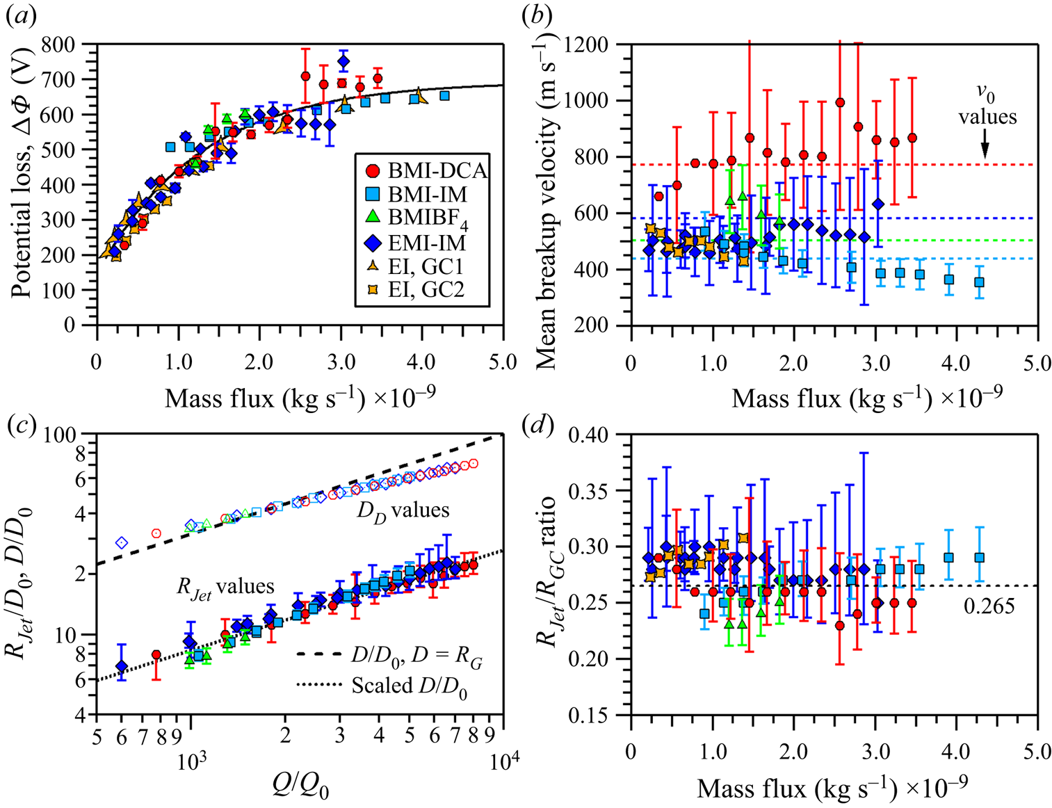
Figure 10. Illustrated electrospray data of the high m/q distribution partly listed in table 3; (a) the potential loss along the cone-jet, ΔΦ; (b) the mean breakup velocity; (c) the dimensionless jet radius, R_Jet/D ₀, (filled markers) and dimensionless primary droplet diameter, D_D/D ₀ (open markers); (d) the jet radius normalized with Gañán-Calvo's characteristic radius R_G (Gañán-Calvo et al. Reference Gañán-Calvo, López-Herrera, Herrada, Ramos and Montanero2018). The additional EMI-IM data from Gamero-Castaño (Reference Gamero-Castaño2008b) and Gamero-Castaño and Cisquella-Serra (Reference Gamero-Castaño and Cisquella-Serra2021) are shown for comparison; noted in the legend as GC1 and GC2, respectively. The error bars represent the accuracy of the linear data fit as seen figure 9.

The jet velocity data are illustrated in figure 10(b), but no distinguishable functional form can be identified. Each IL data set appears to operate within a range of velocities and considering the 1σ level uncertainty may suggest a near constant velocity value for each IL. Larger uncertainties are linked to those experiments that did not as finely probe the kinetic energy values (e.g. 50 eV q⁻¹ instead of 25 eV q⁻¹ step sizes). As one example, the EMI-IM velocity derived from experiments with kinetic energy resolution of 25 eV q⁻¹ exhibit smaller 1σ level uncertainties, narrowing the velocity range from 300 to 700 m s⁻¹ down to a range of 400 to 600 m s⁻¹. A source of comparison for the experimentally measured velocity is to make direct evaluation to Gañán-Calvo's characteristic velocity, U_G (Gañán-Calvo & Montanero Reference Gañán-Calvo and Montanero2009; Ponce-Torres et al. Reference Ponce-Torres, Rebollo-Muñoz, Herrada, Gañán-Calvo and Montanero2018). We noted in presenting table 2 that U_G can be scaled by 4.55, which is a factor associated with a radius ratio of 1.89 (R_Drop/R_Jet), to obtain our own characteristic velocity, v ₀. The v ₀ values listed in table 2 and illustrated as dotted lines in figure 10(b) are comparable to the average velocities as well as of the same order as the experimental values, falling within the range of uncertainties of the respective IL. While the widths of the uncertainties support a radius ratio of 1.89, they would also support a number of other potential ratio values. If instead the scale factor is based on the radius ratio associated with the given flow rate and not on a constant, then v ₀ at each IL flow rate can be calculated from scaling U_G by a factor of [2(R_Drop/R_Jet)]²/${\rm \pi}$. When the factor values are plotted with v_Jet/U_G for each IL (figure S5), the values fall within the uncertainty of each v_Jet/U_G value, suggesting a correlation between U_G and v_Jet via the actual R_Drop/R_Jet value. The value discrepancies may be due to over-estimating the portion of ΔΦ that is going directly into the jet kinetic energy and U_G. There have been reports of energy converted to heat in the electrospray process (Gamero-Castaño Reference Gamero-Castaño2010). We will discuss the determination of the actual R_Drop/R_Jet ratios in the paragraphs below.

In figure 10(c), the jet radius, R_Jet, and droplet diameter, D_D, values are presented as dimensionless quantities versus the dimensionless flow rate Q/Q ₀. The R_Jet value is directly determined from the v_Jet values by R_Jet = [Q/(${\rm \pi}$v_Jet)]^1/2; R_Jet values at select flow rates are listed in table 4. The determination of D_D will be discussed in the paragraphs below. Two lines are plotted in figure 10(c) with the dashed line representing D/D ₀, where D = R_{G ,} and the dotted line representing a scaled D/D ₀ of 3.78⁻¹⋅(D/D ₀). The R_G term is Gañán-Calvo's characteristic radius and evaluates as R_G = [ρε ₀Q ³/(γK)]^1/6 (Gañán-Calvo et al. Reference Gañán-Calvo, López-Herrera, Herrada, Ramos and Montanero2018). The 3.78⁻¹ factor accounts for the change to radius and includes an R_Drop/R_Jet ratio of 1.89. The dotted line overlies the jet radius data, suggesting 1.89 is a good correspondence between D/D ₀ and R_Jet/D ₀. However, the data points are scattered about the dotted line and do not lie directly on the line, suggesting there is some variation to the radius ratio, R_Drop/R_Jet. We have already presented in figure 8(a) the results of evaluating the scaling of D/D ₀ using Q/Q ₀. In figure 8(a) these values directly lie on the dashed line. Given the limitations of the TOF technique used here, the analysis methodology and the quality of the data, we cannot definitively determine a droplet diameter directly from the experiment. The electrification and viscous effects will now be considered to determine the impact on R_Drop/R_Jet and the droplet diameter.

Table 4. Parameters used for the primary droplet estimation. Here, R_D is the primary droplet radius associated with the maximum growth rate of the jet perturbation and is equal to D_D/2. ^aAnion emission data point. ILs listed are BMI-DCA – BD, EMI-IM – EI, BMI-IM – BI and BMI-BF₄ – BB.

4.3. Determination of the critical droplet radius

Gamero-Castaño and Hruby (Reference Gamero-Castaño and Hruby2002) and Gamero-Castaño and Cisquella-Serra (Reference Gamero-Castaño and Cisquella-Serra2021) explored the case of equipotential jet breakup evaluating the electrification and viscous effects on the perturbation driving jet breakup. In the case of neat EMI-IM (Gamero-Castaño & Cisquella-Serra Reference Gamero-Castaño and Cisquella-Serra2021), the authors noted that the equipotential breakup is appropriate as the characteristic flow time during breakup significantly exceeded the electrical relaxation time at the flow rates examined. This situation similarly occurs at all flow rates sampled in our work. Given the rapid electrical relaxation times vis-à-vis the characteristic flow time, the surface charge is likely at equilibrium throughout the breakup. Other effects that lead to non-symmetric perturbations and instabilities such as those pertaining to the development of lateral, kink and ramified emission modes may be factors in the jet breakup that are not included in our or the previous authors approach. In the case of the perturbation in an uncharged and inviscid jet, the radius ratio is 1.89 and generally assumed as the ideal ratio of electrospray breakup. Gamero-Castaño engaged in linear instability analysis to determine the growth rate of the perturbation and the associated droplet radius produced from jet breakup; specifically evaluating the case of a perturbation with a positive growth rate and a wavelength λ yields the associated droplet radius as ${R_{Drop}} = {[(3/4)\lambda R_{Jet}^2]^{1/3}}$. At the maximum growth rate, the perturbation will generate droplets at a critical radius of R_D. Applying the analysis requires understanding that increasing electrification in the jet will result in a destabilizing effect while increasing viscosity has a stabilizing impact. This means that the initial growth rate σ is a function of the perturbation wavenumber (e.g. wavelength), electrification and viscosity. The measure of jet electrification is expressed by the dimensionless Taylor number

(4.5)\begin{equation}\varPsi \cong \frac{{{\alpha ^2}{\beta ^3}}}{4}{\left( {\frac{Q}{{{Q_0}}}} \right)^{1/2}},\end{equation}

where α is the scaling of I/I ₀ = α(Q/Q ₀)^1/2. We assign α = 2.6 based on the fit of measurements for a large group of liquids including EMI-IM (Gañán-Calvo et al. Reference Gañán-Calvo, López-Herrera, Herrada, Ramos and Montanero2018). The β term is simply the ratio of the jet radius normalized by Gañán-Calvo's characteristic radius, β = R_Jet/R_G. This ratio is plotted versus the mass flux in figure 10(d) with the 1.89 ratio noted as the dotted line at ~0.265. The value remains roughly constant with flow rate, ranging in value from 0.23 to 0.32, which represents an approximate spread from the 0.265 value (dotted line) of ±15 %. As Gamero-Castano noted, the geometry of the transition region of the cone-jet is invariant to changing flow rate and with a near constant dimensionless jet radius, the invariance extends from the transition region to the jet breakup. The viscous effect is provided by the dimensionless viscous parameter J

(4.6)\begin{equation}J \cong \beta {\left( {\frac{Q}{{{Q_0}}}} \right)^{1/2}}Re_K^2.\end{equation}

For J, Re_K is another dimensionless quantity that can be determined from Re_K = [ρε ₀γ ²/(μ ³K)]^1/3. Both the Taylor number and J are provided in table 4 for select flow rates. Only three values of J were used for the analysis as Gamero-Castaño has noted the values of J do not have a significant impact for liquids with these electrical conductivities and Taylor numbers; the same wavenumber was obtained regardless of the J value. Additionally, the wavenumber x expressed in terms of wavelength is x = 2${\rm \pi}$(R_Jet/λ). The growth rate σ(x, J, Ψ) of a perturbation is evaluated by a system of two equations of

(4.7)\begin{gather}\sigma \frac{{\rho R_{Jet}^2}}{\mu } = {y^2} - {x^2},\end{gather}

(4.8)\begin{gather}\begin{array}{ccccc} & 2{x^2}({x^2} + {y^2})\dfrac{{{{I^{\prime}}_1}(x)}}{{{I_0}(x)}}\left[ {1 - \dfrac{{2xy}}{{{x^2} + {y^2}}}\dfrac{{{I_1}(x){{I^{\prime}}_1}(y)}}{{{{I^{\prime}}_1}(x){I_1}(y)}}} \right] - ({x^4} - {y^4})\\ & \quad = J\left\{ {x(1 - {x^2})\dfrac{{{I_1}(x)}}{{{I_0}(x)}} - \varPsi \dfrac{{x{I_1}(x)}}{{{I_0}(x)}}\left[ {1 + \dfrac{{x{{K^{\prime}}_0}(x)}}{{{K_0}(x)}}} \right]} \right\} \end{array}\end{gather}

and requires eliminating the y-term. Again, (4.7) and (4.8) consider only an axisymmetric breakup mode and no other effects on the electrospray system. The associated wavenumber at the maximum growth rate x* is extracted from this system. Thus, the wavelength λ* at the maximum growth rate yields the critical droplet radius of R_D

(4.9)\begin{equation}\frac{{{R_D}(J,\mathrm{\Psi })}}{{{R_{Jet}}}} = {\left( {\frac{3}{4}\frac{{{\lambda^\ast }}}{{{R_{Jet}}}}} \right)^{1/3}}.\end{equation}

The values of R_D and R_D/R_Jet are listed in table 4 for select flow rates. Note that the R_D/R_Jet values range between 1.5 and 2.3, which is indicative of the value for all the flow rates and ILs studied. This analysis indicates that the IL electrosprays studied here do not breakup with the same value found for an uncharged and inviscid system. Figure 10(c) presents the generated droplets in terms of diameter, D_D. The dimensionless droplet diameters overlap the line of D/D ₀, but do not quantitatively overlie this line. The droplet diameter significantly deviates from D/D ₀ at the largest flow rates for all ILs measured and can be attributed to the influence of the breakup wavelength on the system. Deviation from D/D ₀ starts near the Q/Q ₀ value of 2147 corresponding to the Rayleigh limit associated with the scaling law presented earlier in figure 8. For our data, a Taylor number of approximately Ψ = 1.54 represents the point that the jet electrification term reaches the Rayleigh limit. As shown in the table 4 for all four ILs, the Taylor number exceeds this value around a Q/Q ₀ value of 2000. Non-symmetric perturbations could be a factor in breakup once the appropriate flow rate and Rayleigh limit are reached. These perturbations are not considered in this study. The evaluation of (4.9) for the four neat ILs finds that the electrification and viscous effects are a factor that must be considered in the electrospray analysis. For R_Drop = R_D, the values of m, q_Ray and m/q_Ray of the primary droplet for each IL and flow rate can be determined. These values are also listed in table 4 for select flow rates. The droplet mass and Rayleigh limit are calculated via (4.1) and (4.2). These primary droplets have mass values spanning the range of 0.5 × 10⁸ to 15.0 × 10⁸ amu and are capable of carrying hundreds of charges. BMI-IM electrosprays generate primary droplets with the most mass over the flow regime.

4.4. Modelling the jet breakup and droplet characteristics

The data presented with figures 2–5 clearly indicate that the mass spectrum is significantly more complicated than the simple estimation of the mean m/q value. A diversity of m/q values is measured within the experimental data and volumetric flow rates are examined that expect the mean droplet to have a charge exceeding the Rayleigh charge limit (see figure 8b). The measurement of the species at specific potential values facilitates a deeper understanding of the variance in the breakup potential and jet velocity or, alternatively, a reflection of the dynamics occurring as the ion beam propagates downstream away from the jet. The smoothed fits to the droplet component of the mass spectrum in figure 4 demonstrate that a common m/q value is represented in multiple stopping potential values. Figure 11(a) presents the intensity of selected m/q values, in 50 amu q⁻¹ bins, between 100 000 to 500 000 for BMI-IM at a flow rate of 0.96 nl s⁻¹ (Q/Q ₀ = 1620) as a function of the base DC potential. The intensity of a specific m/q value often spans more than 100 V and all distributions sampled are well modelled with a Gaussian functional form. Figure 11(b) provides the statistical outputs of the fitting including the mean potential for the specific m/q value and the FWHM value describing the potential width. A variation of the FWHM from low to high mass-to-charge, increasing in value, is observed in every data set examined in this work.

Figure 11. (a) Intensity of selected m/q values as a function of the base plate potential. (b) Statistical outputs of Gaussian fits to the distributions. FWHM values are offset in x by 25 000.

The variance in the FWHM values with respect to m/q indicates that the kinetic energy properties of the droplets in the emitted beam originating from the jet cannot be exclusively attributed to only subtle variations in the length of the jet. Small length variations would be expected to expose the jet breakup to slightly different breakup potentials. As the jet breakup potential is independent of m/q in (4.3), small variations in breakup potentials should result in identical FWHM distribution widths in figure 11(b) for all m/q values. A diversity of jet velocities should also have a significant effect on the resulting kinetic energy distribution. According to (4.3), small changes are more likely to have more significant impacts on the larger m/q values as it pertains to the E/q widths. Doubling of the m/q value with any velocity width chosen should result in a doubling of the width of the E/q distribution. A comparison of the 200 000 and 400 000 amu q⁻¹ FWHM values in figure 11(b) gives values of 95 and 140 V, respectively. The data do not support either the velocity or length distribution being unilaterally responsible for the resulting kinetic energy profiles of the charged species. Under the assumption that in-flight, charge-repulsion dynamics has a minimal role in the resulting axial kinetic energies of the ions, we examine what variations in jet parameters are necessary so as to reproduce the measured distributions.

Twelve data sets of BMI-IM at various flow rates were analysed similarly to the analysis shown in figure 11. For each data set, the intensity versus potential of slices every 25 000 amu q⁻¹ from 100 000–600 000 amu q⁻¹ were examined and the centre and FWHM values at each m/q value were recorded. First, (4.3) was used to find the v_Jet and Φ_Jet that minimized the error in reproducing the E/q (potential, V) value expected for a specific m/q point (i.e. the black circles in figure 11b). To reproduce the width of the distribution, a value for the variance in the jet velocity and potential (v_unc and Φ_unc, respectively) was used. A custom script was generated that modelled these uncertainties numerically in which v_unc or Φ_unc served as the standard deviation of a Gaussian distribution from which random values would be selected. The expected axial kinetic energies of 5 million charged species per m/q value were populated through this random selection from each of these distributions individually which were then added to their respective v_Jet or Φ_Jet value. A histogram was generated from the resulting ensemble and the resulting Gaussian distribution (a function of E/q) was fit. The output FWHM values of this simulation were compared directly with the experimental FWHM values. The validity of the variance values was assessed by minimizing the sum of the chi square values determined for each individual m/q value in a given data set. The values of the individual data sets are given in the supplemental information (table S1) while the statistical output values for all of the data sets are now discussed. The average of v_unc was found to be 27.4 ± 1.5 m s⁻¹ (1σ) and Φ_unc = 33.9 ± 3 V (1σ) for all sets examined. In the limit that the jet dynamics is the only contributor to the distributions, the variance of velocity of the jet predicts droplet diameters that have standard deviations of approximately 6 % (and droplet mass by approximately 9 %). This estimation of droplet diameter variance is in good agreement with the work of Gamero-Castaño (Reference Gamero-Castaño2010), which noted that a standard deviation of the ensemble of droplet diameters was approximately 6 %–7 % while the standard deviation of the charge was 17 %–22 % for an EMI-IM solution dissolved in propylene carbonate.

A significant limitation of the TOF experiments described in this report is the inability of the system to differentiate the specific mass and specific charge of the individual droplets. The analysis of the results is thus limited to the ability to infer information directly from the mass-to-charge ratio of the detected species and to apply previously validated approaches, such as the empirical scaling laws frequently described above. We define primary droplets as those that compose the bulk of the mass emitted from the end of the jet and represent the droplet expected from the jet with approximate radius given by (4.9). The bulk of the individual points shown in figures 9 and 11 is for droplets that have charge values that would be super-Rayleigh if the only droplets emitted are these primary droplets. We will refer to satellite droplets as those other droplets, such as those with mass-to-charge values below the Rayleigh limit of the primary droplet, which originate from either the remnants of the jet not incorporated in the primary droplet or some additional dynamical process involving subsequent breakup of the primary droplet.

Six exemplar kinetic energy-integrated mass-to-charge distributions for BMI-IM at 0.54, 0.95 and 1.88 nl s⁻¹ and EMI-IM at 0.14, 0.72 and 1.13 nl s⁻¹ are shown in figure 12. We choose to focus on the mass spectrum data from the lower volumetric flow rates because there is minimal expected current loss to the extractor plate and the effect of plume divergence on the analysis is expected to be minimized (Miller et al. Reference Miller, Prince, Bemish and Rovey2014). The integrated spectrum (black/grey) is generated by binning each kinetic energy specific spectrum into 500 amu q⁻¹ bins and then summing the individual transformed spectra at each specific kinetic energy. The vertical dashed lines indicate the lowest m/q value at which the primary droplet is expected to survive assuming R_D in table 4; those primary droplets with mass-to-charge ratios to the left of the vertical line would be super-Rayleigh and those to the right would be sub-Rayleigh. These composite spectra demonstrate that if only primary droplets were present, nearly every counted species would have charge values exceeding the Rayleigh limit. In an attempt to identify characteristics of the droplets that are measured within a requirement to balance emitted mass and charge in the complete beam, we explored a model that treats the composite spectrum as being composed of three distinct masses. In this ‘Model 1’, the component at the largest m/q values is considered the primary droplet with its mass and associated Rayleigh limit calculated directly from values in table 4. Any ions with mass-to-charge values occurring below the mass-to-charge associated with the Rayleigh limit were directly added to a second distribution, the large droplet (a satellite droplet). This transfer of population from primary to large is not shown in figure 12. A third distribution, associated with the smallest charged species was also included (small droplet). Finally, any counted event occurring below 7000 amu q⁻¹ was taken to be a singly charged ion with mass equal to the mass-to-charge value. The mass values of the large droplet and small droplet were taken as fit parameters and their respective Rayleigh limits were calculated and recursively solved. For those charged species with mass-to-charge values less than the m/q_Ray value of the large droplet, the intensity would be directly added to the small droplet distribution. As an example of the division in these values, the EMI-IM data in figure 12 have three vertical lines that delineate the boundary between the primary droplet and large droplet (dashed), the large droplet and small droplet (dot-dash) and the small droplet and ions (dot). These lines are the result of the best fits approach described in the paragraph below. The charge for each droplet distribution at a given m/q was determined by division of the respective droplet mass value by the m/q value associated with the specific bin. We must also note that the small droplet component is subject to some overlap with the low m/q droplet distribution, which will lead to larger uncertainties in its values.

Figure 12. Kinetic energy integrated mass spectrum for EMI-IM and BMI-IM at six flow rates. Dashed line indicates the expected m/q_Ray value of the primary droplet, the dash-dot line indicates the m/q_Ray value of the large droplet while the dotted line indicates the m/q_Ray value of the small droplet.

Under the assumption that the detector efficiency is approximately identical for all droplets measured (Fontanese et al. Reference Fontanese, Clark, Horányi, James and Sternovsky2018; Gemer et al. Reference Gemer, Sternovsky, James and Horanyi2020; Llera et al. Reference Llera, Burch, Goldstein and Goetz2020), the total mass and total charge measured can be estimated by multiplication of the counts by the respective (mass and charge) value for all species counted in the mass spectrum. These values are then added to the mass and charge expected from the singly charged ions, which contribute little to both summed values. The composite summed mass value is multiplied by a constant so as to reproduce the mass flow of the entire beam as determined from the volumetric flow rate. This constant then multiplies the summed charge value and an evaluation of the deviation of total modelled charge from total emitted charge is undertaken. Treatment of the entire measured spectrum as primary droplets results in mean charge errors of +192 % when analysed in this way. Application of the described approach in Model 1 to 12 data sets from EMI-IM and BMI-IM results in mean unsigned errors in the charge of 10.5 % with a general overestimation of charge in the BMI-IM cases (+3.0 to +27.6 % at the extremes) and 8.5 % in the EMI-IM cases (−14.0 to +9 % signed errors at the extremes). We speculate that the EMI-IM analysis performs better than BMI-IM analysis because BMI-IM has droplets with larger m/q values and that our detector efficiency must be less for these high mass with lower relative charge value species.

A selection of the results for the Model 1 analysis of BMI-IM and EMI-IM are given in table 5 for the primary, large and small droplets. While specific values for mass and charge are given, the jet velocity analysis indicated that emitted species will have some width to their values. Since the mass of each component droplet is fixed in this analysis, the width of the distribution is ultimately reflected in the charge range. The range of charges are the values expected for the middle 80 % of droplets with the given mass. As noted in the introduction of Model 1 above, the primary droplet distribution is not allowed to extend to lower m/q values than the m/q_Ray value. The part of the distribution that would exceed is directly added to the large droplet component. The primary droplets exhibit charge values mostly concentrated near the Rayleigh limit with the range expanding, on an absolute basis, as the flow rate increases. The width of the charge distribution typically constitutes 14 %–28 % of the Rayleigh limit. In the case of EMI-IM, the large droplet component is 25.3 % (±3 %) of the mass of the primary droplet while the small droplet is smaller and comprises only 9.9 % (±5.3 %) of the same mass. For the average values of six flow rates of EMI-IM analysed with Model 1, the primary droplet made up 21 ± 6 % of the total counted species above ~50 000 amu q⁻¹ while the large droplet is 55 ± 7 % and the small droplet is 22 ± 5 %. The species above 50 000 amu q⁻¹ range from approximately 16 % to 56 % of the total counted events in the EMI-IM mass spectrum. The individual ions and the low m/q components make up the remainder. At Q = 1.13 nl s⁻¹, the primary droplets carry ~45 % of the mass and 30 % of the charge while the large droplets carry ~53 % and 62 %, respectively.

Table 5. Model 1 analysis results from selected liquids and flow rates for EMI-IM (EI) and BMI-IM (BI). Here, m is given in amu, q is given in integer charges and represents the range in which the middle 80 % of the charge is contained and q_Ray is the Rayleigh charge of the primary droplet. Pri, primary droplet; Lg, large droplet; and Sm, small droplet.

The BMI-IM data are considerably different when the same analysis is employed to find the mass of the large and small droplet components. When the error in measured charge is quantified, the result with minimized charge error is to simply exclude a multi-component fit to the spectrum, with the exception of the primary droplet and one additional droplet component. Low m/q droplets and ions are still measured and do contribute as well, although they are not quantified in table 5. The best fits are accomplished for all flow rates sampled by establishing a small mass droplet with values of the order of 10⁵ amu. In terms of number of events, these small mass droplets dominate the spectrum, often contributing more than 80 % of the total charged species events recorded. As a result of their low mass and the broad m/q range covered, the bulk of their charge range is measured in the low integer number of charges. At Q = 1.13 nl s⁻¹, the primary droplets carry ~95 % of the total mass and ~90 % of the total charge in the error minimized Model 1 result.

Our interpretation of the results has relied on the analysis of a number of different measured quantities in the experiment that will be briefly summarized here. With exception of the low m/q distribution of species and a small percentage of the intensity of small ions, the emitted electrospray beam appears to be completely reconcilable with direct emission from the jet tip with allowance for some variation in the velocity and breakup point. Droplets with m/q values below the Rayleigh limit cutoff for the predicted primary droplets are observed in the mass spectrum. Assuming the high m/q contributors to the mass spectrum carry essentially all the mass and charge of the beam, mass and charge measured downstream can be conserved to the near-field measurements (when properly multiplied by a common constant) by treating the high m/q component with a number of distinct distributions in which the primary droplet makes up the component at the higher m/q values and considerably smaller mass (and charge) components compose the rest of the observed total distribution. In this framework, the jet emits a number of massive primary droplets and a significantly larger quantity of satellite droplets. Because the kinetic energy profile of these satellite droplets behaves similarly to the primary droplets, it is difficult to ascribe their generation to Coulomb explosions of the primary droplets unless it occurs within extremely short time scales so as to appear with potential values that approximate the breakup region of the jet. Additionally, our data cannot exclude the case of the satellite droplets forming in the actual jet breakup as left over mass and charge.

The kinetic energy behaviour of the low m/q distribution, demonstrated for example in figure 3(a) and figure S2 (supplemental), significantly deviates from the remainder of the components previously addressed. If values from the low m/q distribution were added to the data presented in figure 9, it would generate a series of points well represented by a vertical line around an x-value of 1.3 × 10⁻⁴ kg C⁻¹. This anomalous behaviour is not easily reconciled by changes in jet velocity or breakup potential. We believe the generation of this component should be ascribed to Coulombic breakup of some component in the post-jet ion beam described above. The nearly identical m/q distribution appearing over a broad kinetic energy range is indicative that these species cannot directly originate from the jet. The wide variability of kinetic energies for common m/q values is the result of the cast-off (or Coulomb explosion) event occurring with variable time scales post-emission. These cast-off droplets experience different lengths of time exposed to the electric field at their final mass-to-charge value, generating a diversity of different resulting energy defects. This would agree with recent measurements of EMI-IM at similar flow rates by Gamero-Castaño and Cisquella-Serra (Reference Gamero-Castaño and Cisquella-Serra2021) who ascribed anomalous behaviour by low mass-to-charge species as resulting from Coulombic explosion of droplets with significant charge values. To estimate the size of these cast-off species we turn to the highest resolution spectrum that was generated for BMI-IM, presented in figure S3. This spectrum shows a progression ascribable to ions with small q values that becomes un-resolvable when q reaches 4–5 charges but clearly extends to larger m/q values with the most significant intensity around 20 000 amu q⁻¹, consistent with the values of the low m/q distribution measured. At the apparent maximum, if q were ‘5’, the resulting mass would be approximately 100 000 amu and the associated radius would be ~3.0 nm. Whether such species should be arbitrarily labelled ‘ions’ or ‘droplets’, we note that low m/q distributions are present and the kinetic energy behaviour is similar at all flow rates, including those where the mean primary droplet is not expected to exceed the Rayleigh limit but our assessment of the charge distribution includes some primary droplets that would.