


1 Introduction
The study of a turbulent boundary layer (hereafter denoted TBL) over a smooth wall at an ever increasing Reynolds number (
 $Re$
) is motivated by the expectation that as
$Re$
) is motivated by the expectation that as
 $Re$
increases, the boundary layer approaches an ‘asymptotic’ or
$Re$
increases, the boundary layer approaches an ‘asymptotic’ or
 $Re$
-independent state. This would correspond to the ideal situation, where the viscous-dominated near-wall region is absent. Based on a self-preservation analysis (Townsend Reference Townsend1956, Reference Townsend1976), the mean velocity and Reynolds shear stress profiles can then be normalised using one velocity scale and one length scale. However, this asymptotic state of a smooth wall TBL is unlikely to be reached. First, it is impossible to achieve extremely high
$Re$
-independent state. This would correspond to the ideal situation, where the viscous-dominated near-wall region is absent. Based on a self-preservation analysis (Townsend Reference Townsend1956, Reference Townsend1976), the mean velocity and Reynolds shear stress profiles can then be normalised using one velocity scale and one length scale. However, this asymptotic state of a smooth wall TBL is unlikely to be reached. First, it is impossible to achieve extremely high
 $Re$
in a laboratory, thus preventing the possibility of investigating a
$Re$
in a laboratory, thus preventing the possibility of investigating a
 $Re$
-independent TBL, or a TBL with negligible viscous effects in the near-wall region (such that the viscous term in the equations of motion can be neglected in comparison to the other terms). Second, from an experimental point of view, if one increases
$Re$
-independent TBL, or a TBL with negligible viscous effects in the near-wall region (such that the viscous term in the equations of motion can be neglected in comparison to the other terms). Second, from an experimental point of view, if one increases
 $Re$
to very large values, the TBL is unlikely to develop over a hydrodynamically smooth wall. This is because the thickness of viscosity-dominated near-wall layer decreases as
$Re$
to very large values, the TBL is unlikely to develop over a hydrodynamically smooth wall. This is because the thickness of viscosity-dominated near-wall layer decreases as
 $Re$
increases. While no smooth wall TBL study has been carried out with an indefinitely increasing Reynolds number, it is expected that at some critical value of
$Re$
increases. While no smooth wall TBL study has been carried out with an indefinitely increasing Reynolds number, it is expected that at some critical value of
 $Re$
, this layer would become so thin that any imperfections of the surface would act as roughness. It should be noted that we are considering the case where
$Re$
, this layer would become so thin that any imperfections of the surface would act as roughness. It should be noted that we are considering the case where
 $Re$
is increased by increasing the free stream velocity and/or decreasing the kinematic viscosity. If one keeps these parameters constant and moves along the wall,
$Re$
is increased by increasing the free stream velocity and/or decreasing the kinematic viscosity. If one keeps these parameters constant and moves along the wall,
 $Re$
increases but also the viscous scale. Consequently, a TBL over a nominally smooth wall will experience a continuous change in the wall roughness (inner-normalised roughness) as
$Re$
increases but also the viscous scale. Consequently, a TBL over a nominally smooth wall will experience a continuous change in the wall roughness (inner-normalised roughness) as
 $Re$
increases and will evolve from a smooth regime to a fully rough regime.
$Re$
increases and will evolve from a smooth regime to a fully rough regime.
It is generally accepted (Hinze Reference Hinze1975) that for the fully rough regime, the effect of viscosity in the near-wall region becomes negligible (on a spatially averaged basis) and the coefficient of friction becomes independent of
 $Re$
. This could present an interest if such a fully rough TBL can be interpreted as a surrogate to a smooth wall TBL with no viscous sublayer. Such a comparison may be possible if Townsend’s wall similarity hypothesis or Townsend’s Reynolds number similarity hypothesis (Townsend Reference Townsend1956, Reference Townsend1976) is valid. This hypothesis states that ‘outside the viscous layer (region close to the surface) lies a region of fully turbulent flow, where the viscous stresses are small compared with the Reynolds stresses’ and the outer flow is in a state of self-similarity. This outer region is thus thought to be nearly independent of viscosity of the fluid and determined by the wall shear stress and the channel width, pipe diameter or boundary layer thickness. Accordingly, if, at a moderate
$Re$
. This could present an interest if such a fully rough TBL can be interpreted as a surrogate to a smooth wall TBL with no viscous sublayer. Such a comparison may be possible if Townsend’s wall similarity hypothesis or Townsend’s Reynolds number similarity hypothesis (Townsend Reference Townsend1956, Reference Townsend1976) is valid. This hypothesis states that ‘outside the viscous layer (region close to the surface) lies a region of fully turbulent flow, where the viscous stresses are small compared with the Reynolds stresses’ and the outer flow is in a state of self-similarity. This outer region is thus thought to be nearly independent of viscosity of the fluid and determined by the wall shear stress and the channel width, pipe diameter or boundary layer thickness. Accordingly, if, at a moderate
 $Re$
, the effect of viscosity in the near-wall region of the boundary layer is removed or made negligible on a spatially averaged basis (Talluru et al.
Reference Talluru, Djenidi, Kamruzzaman and Antonia2016), then, according to the Reynolds number similarity, the boundary layer behaviour at that
$Re$
, the effect of viscosity in the near-wall region of the boundary layer is removed or made negligible on a spatially averaged basis (Talluru et al.
Reference Talluru, Djenidi, Kamruzzaman and Antonia2016), then, according to the Reynolds number similarity, the boundary layer behaviour at that
 $Re$
can be expected to be similar to that of a smooth wall boundary layer in the asymptotic state of
$Re$
can be expected to be similar to that of a smooth wall boundary layer in the asymptotic state of
 $Re$
.
$Re$
.
There are numerous studies on rough wall flows reported in the literature which tested the validity of Townsend’s hypothesis regarding the universal behaviour of the outer region of smooth and rough wall turbulent boundary layers. In the context of three-dimensional roughness, Flack, Schultz & Shapiro (Reference Flack, Schultz and Shapiro2005), Volino, Schultz & Flack (Reference Volino, Schultz and Flack2007), Squire et al. (Reference Squire, Morrill-Winter, Hutchins, Schultz, Klewicki and Marusic2016) and references therein provide clear support to that hypothesis, at least when the ratio of roughness height (
 $k$
) to boundary layer thickness (
$k$
) to boundary layer thickness (
 $\unicode[STIX]{x1D6FF}$
) is small. Similar observations are made in turbulent flows over two-dimensional roughness (Krogstad & Efros Reference Krogstad and Efros2012, spanwise square bars) and three-dimensional roughness (Raupach Reference Raupach1981; Amir & Castro Reference Amir and Castro2011). In contrast, there are other studies that reported differences in the outer layer region of smooth and rough wall flows (for example, Krogstad, Antonia & Browne Reference Krogstad, Antonia and Browne1992; Tachie, Bergstrom & Balachandar Reference Tachie, Bergstrom and Balachandar2000; Leonardi et al.
Reference Leonardi, Orlandi, Smalley, Djenidi and Antonia2003; Bhaganagar, Kim & Coleman Reference Bhaganagar, Kim and Coleman2004; Lee & Sung Reference Lee and Sung2007), raising a possible outer layer controversy as discussed by Antonia & Djenidi (Reference Antonia and Djenidi2010). While this issue is not yet fully addressed, it is argued that the conflicting findings are often attributed to the large ratio
$\unicode[STIX]{x1D6FF}$
) is small. Similar observations are made in turbulent flows over two-dimensional roughness (Krogstad & Efros Reference Krogstad and Efros2012, spanwise square bars) and three-dimensional roughness (Raupach Reference Raupach1981; Amir & Castro Reference Amir and Castro2011). In contrast, there are other studies that reported differences in the outer layer region of smooth and rough wall flows (for example, Krogstad, Antonia & Browne Reference Krogstad, Antonia and Browne1992; Tachie, Bergstrom & Balachandar Reference Tachie, Bergstrom and Balachandar2000; Leonardi et al.
Reference Leonardi, Orlandi, Smalley, Djenidi and Antonia2003; Bhaganagar, Kim & Coleman Reference Bhaganagar, Kim and Coleman2004; Lee & Sung Reference Lee and Sung2007), raising a possible outer layer controversy as discussed by Antonia & Djenidi (Reference Antonia and Djenidi2010). While this issue is not yet fully addressed, it is argued that the conflicting findings are often attributed to the large ratio
 $k/\unicode[STIX]{x1D6FF}$
(Jiménez Reference Jiménez2004) used in some studies, wherein, a significant region of the boundary layer is directly influenced by the roughness. Jiménez (Reference Jiménez2004) suggests that there is a need for additional experiments in fully rough flows with large equivalent sand-grain roughness (
$k/\unicode[STIX]{x1D6FF}$
(Jiménez Reference Jiménez2004) used in some studies, wherein, a significant region of the boundary layer is directly influenced by the roughness. Jiménez (Reference Jiménez2004) suggests that there is a need for additional experiments in fully rough flows with large equivalent sand-grain roughness (
 $k_{s}^{+}>100$
) and small relative roughness height (
$k_{s}^{+}>100$
) and small relative roughness height (
 $\unicode[STIX]{x1D6FF}/k>40$
) in order to properly test Townsend’s hypothesis. For a relatively recent account on wall-bounded turbulent flows over rough walls, the interested reader can consult Nickels (Reference Nickels2010).
$\unicode[STIX]{x1D6FF}/k>40$
) in order to properly test Townsend’s hypothesis. For a relatively recent account on wall-bounded turbulent flows over rough walls, the interested reader can consult Nickels (Reference Nickels2010).
A common point that is conspicuously absent in all rough wall turbulent flow studies is a discussion on how different roughnesses can have different effects on the near-wall viscous region. In particular, it is not clear how the effects of viscosity in the near-wall region are altered (increased or dampened) by the roughness and how this alteration, which may be different for different roughness geometries, affects the flow dynamics. Further, there are no previous studies that report the effects of the removal (or weakening) of the near-wall viscosity-dominated layer on the development of the TBL and how such a TBL behaves with increasing
 $Re$
. Thus, the novelty of the present study relates to the idea that by changing the boundary condition one can essentially get rid of the dampening effects of the viscosity in the near-wall region, which allows the boundary layer to grow faster than on a smooth wall, thus providing a method of ‘simulating’ high Reynolds number TBL, particularly in a low speed wind tunnel. Further, the ability to generate a TBL where the near-wall viscous effects are negligible, if not removed, provides the ideal conditions required to investigate Townsend’s Reynolds number similarity hypothesis.
$Re$
. Thus, the novelty of the present study relates to the idea that by changing the boundary condition one can essentially get rid of the dampening effects of the viscosity in the near-wall region, which allows the boundary layer to grow faster than on a smooth wall, thus providing a method of ‘simulating’ high Reynolds number TBL, particularly in a low speed wind tunnel. Further, the ability to generate a TBL where the near-wall viscous effects are negligible, if not removed, provides the ideal conditions required to investigate Townsend’s Reynolds number similarity hypothesis.
A practical and relatively simple method for removing or significantly reducing the viscosity effect in the near-wall region of a TBL at a moderate
 $Re$
is to introduce roughness elements. In particular, a roughness consisting of transverse rods attached to the wall is quite effective for achieving a fully rough regime where the viscous drag is negligible or zero at relatively low
$Re$
is to introduce roughness elements. In particular, a roughness consisting of transverse rods attached to the wall is quite effective for achieving a fully rough regime where the viscous drag is negligible or zero at relatively low
 $Re$
. Leonardi et al. (Reference Leonardi, Orlandi, Smalley, Djenidi and Antonia2003) showed that a channel flow with a surface roughness made of periodic two-dimensional (2-D) transverse square bars has practically no (global) viscous drag when the spacing between two consecutive roughness elements is varied between 8 and 16 times the roughness height; the drag is almost entirely made up of form drag. Similar observations were made in the numerical simulation of a channel flow with 2-D circular rods as the roughness elements (Leonardi et al.
Reference Leonardi, Orlandi, Djenidi and Antonia2015). In a recent experimental study, Kamruzzaman et al. (Reference Kamruzzaman, Djenidi, Antonia and Talluru2015) measured the form drag directly using the static pressure distribution around a single circular rod on a 2-D rough wall (same as the current study) and found that the coefficient of friction becomes independent of
$Re$
. Leonardi et al. (Reference Leonardi, Orlandi, Smalley, Djenidi and Antonia2003) showed that a channel flow with a surface roughness made of periodic two-dimensional (2-D) transverse square bars has practically no (global) viscous drag when the spacing between two consecutive roughness elements is varied between 8 and 16 times the roughness height; the drag is almost entirely made up of form drag. Similar observations were made in the numerical simulation of a channel flow with 2-D circular rods as the roughness elements (Leonardi et al.
Reference Leonardi, Orlandi, Djenidi and Antonia2015). In a recent experimental study, Kamruzzaman et al. (Reference Kamruzzaman, Djenidi, Antonia and Talluru2015) measured the form drag directly using the static pressure distribution around a single circular rod on a 2-D rough wall (same as the current study) and found that the coefficient of friction becomes independent of
 $Re$
. Similar results were reported by Bakken et al. (Reference Bakken, Krogstad, Ashrafian and Andersson2005) in a rod-roughened turbulent channel flow. All these experimental and numerical results indicate that the spatially averaged viscous friction becomes zero, or at least negligible in comparison to form drag. In other words, the flow becomes fully rough. Interestingly, the
$Re$
. Similar results were reported by Bakken et al. (Reference Bakken, Krogstad, Ashrafian and Andersson2005) in a rod-roughened turbulent channel flow. All these experimental and numerical results indicate that the spatially averaged viscous friction becomes zero, or at least negligible in comparison to form drag. In other words, the flow becomes fully rough. Interestingly, the
 $Re$
-independence of the friction coefficient (
$Re$
-independence of the friction coefficient (
 $C_{f}$
) is consistent with the Reynolds number similarity hypothesis and suggests that this hypothesis can be satisfied everywhere within a self-preserving turbulent boundary layer for which
$C_{f}$
) is consistent with the Reynolds number similarity hypothesis and suggests that this hypothesis can be satisfied everywhere within a self-preserving turbulent boundary layer for which
 $C_{f}$
is constant. This possibility is investigated here.
$C_{f}$
is constant. This possibility is investigated here.
The present paper reports measurements made in a TBL which develops over a rough wall. The aim of the study is to assess the behaviour of the (rough wall) TBL as
 $Re$
increases with the view to determining whether a
$Re$
increases with the view to determining whether a
 $Re$
-independent state can be achieved at a moderate
$Re$
-independent state can be achieved at a moderate
 $Re$
. This objective is of great interest from both fundamental and practical viewpoints because it should help to address the following issues:
$Re$
. This objective is of great interest from both fundamental and practical viewpoints because it should help to address the following issues:
(i) Is there a universal asymptotic or
 $Re$
-independent state for a TBL? If so, does this lead to a collapse of all normalised mean velocity profiles, for example?
$Re$
-independent state for a TBL? If so, does this lead to a collapse of all normalised mean velocity profiles, for example?(ii) Is the Reynolds number similarity valid or possible at moderate Reynolds numbers?
(iii) Can a fully rough wall TBL be used as a surrogate to a smooth wall TBL at extremely large
$Re$
.(iv) What is the dynamical behaviour of an asymptotic TBL?


Evidently, care has to be exercised when extrapolating results obtained in a rough wall TBL at moderate
 $Re$
to a smooth wall TBL in the asymptotic state of
$Re$
to a smooth wall TBL in the asymptotic state of
 $Re$
. Indeed, the physical mechanism which helps remove the effect of viscosity in the near-wall region of a rough wall TBL is most likely different to that over a smooth wall when the state of
$Re$
. Indeed, the physical mechanism which helps remove the effect of viscosity in the near-wall region of a rough wall TBL is most likely different to that over a smooth wall when the state of
 $Re$
-independency is achieved. Issue (i) has an important implication for the prediction/estimation of some quantities. Indeed, the existence of a universal state can be exploited for developing models, such as the Clauser chart to estimate the friction coefficient, or the spectral chart developed by Djenidi & Antonia (Reference Djenidi and Antonia2012) for estimating the turbulent kinetic energy dissipation rate. Issue (iv) is relevant for TBL control; in this context, it is important to ascertain how a
$Re$
-independency is achieved. Issue (i) has an important implication for the prediction/estimation of some quantities. Indeed, the existence of a universal state can be exploited for developing models, such as the Clauser chart to estimate the friction coefficient, or the spectral chart developed by Djenidi & Antonia (Reference Djenidi and Antonia2012) for estimating the turbulent kinetic energy dissipation rate. Issue (iv) is relevant for TBL control; in this context, it is important to ascertain how a
 $Re$
-independent TBL responds to perturbations, e.g. wall suction, wall blowing, large eddy break up devices (LEBUs), wall roughness and whether a control strategy can be
$Re$
-independent TBL responds to perturbations, e.g. wall suction, wall blowing, large eddy break up devices (LEBUs), wall roughness and whether a control strategy can be
 $Re$
independent.
$Re$
independent.
Finally, the idea that different asymptotic states may be associated with different boundary and/or initial conditions is not new. For example, George (Reference George1989) discussed the effect of initial conditions and coherent structures on the self-preservation states in various turbulent free shear flows (e.g. jets, wakes). Krogstad & Antonia (Reference Krogstad and Antonia1999) discussed the effects of surface roughness on a TBL by comparing measurements from two different rough surfaces (a woven stainless steel mesh screen and transverse rods) with measurements in a smooth wall TBL (
 $Re_{\unicode[STIX]{x1D703}}=12\,570$
). Unfortunately, only one Reynolds number was considered in each case (
$Re_{\unicode[STIX]{x1D703}}=12\,570$
). Unfortunately, only one Reynolds number was considered in each case (
 $Re_{\unicode[STIX]{x1D703}}=12\,800$
for the mesh screen surface, 4806 for the rod-roughened wall and 12 570 for the smooth wall;
$Re_{\unicode[STIX]{x1D703}}=12\,800$
for the mesh screen surface, 4806 for the rod-roughened wall and 12 570 for the smooth wall;
 $Re_{\unicode[STIX]{x1D703}}$
is the Reynolds number based on the momentum thickness). Also, no study has been reported, where the roughness geometry and the Reynolds number are systematically varied. The present study, which complements and extends the investigation begun by Krogstad & Antonia (Reference Krogstad and Antonia1999), is aimed at filling this knowledge gap.
$Re_{\unicode[STIX]{x1D703}}$
is the Reynolds number based on the momentum thickness). Also, no study has been reported, where the roughness geometry and the Reynolds number are systematically varied. The present study, which complements and extends the investigation begun by Krogstad & Antonia (Reference Krogstad and Antonia1999), is aimed at filling this knowledge gap.
2 Experimental details
Experiments are conducted in a boundary layer wind tunnel which was described in detail in Krogstad et al. (Reference Krogstad, Antonia and Browne1992) and Kamruzzaman et al. (Reference Kamruzzaman, Djenidi, Antonia and Talluru2015). Only the main features of the test section are described here. The test section is 5.4 m long and 0.9 m wide. At the exit of the contraction (6 : 1), the test section has a height of 0.15 m. It is tripped at the contraction exit by a 4 mm diameter rod followed by 170 mm long strip of No. 40 grit sandpaper. Following the contraction, the roof of the test section is adjusted in order to compensate for the growth of the boundary layers and to maintain a zero pressure gradient along the entire working section of the wind tunnel. The pressure gradient is maintained to be within
 $\pm 0.1\,\%$
of the free-stream dynamic pressure. The boundary layer develops over a rough wall, which consists of a periodic arrangement of cylindrical rods mounted on the wall and spanning across the full width of the test section (see figure 1). The diameter (
$\pm 0.1\,\%$
of the free-stream dynamic pressure. The boundary layer develops over a rough wall, which consists of a periodic arrangement of cylindrical rods mounted on the wall and spanning across the full width of the test section (see figure 1). The diameter (
 $k$
) of the rods is nominally 1.6 mm and the spacing (
$k$
) of the rods is nominally 1.6 mm and the spacing (
 $p$
) between the rods is set to
$p$
) between the rods is set to
 $p/k=8$
. In all the experiments, the friction velocity (
$p/k=8$
. In all the experiments, the friction velocity (
 $U_{\unicode[STIX]{x1D70F}}$
) is obtained by integrating the pressure distribution around the roughness element (see Kamruzzaman et al.
Reference Kamruzzaman, Djenidi, Antonia and Talluru2015, for full details). For the virtual origin (
$U_{\unicode[STIX]{x1D70F}}$
) is obtained by integrating the pressure distribution around the roughness element (see Kamruzzaman et al.
Reference Kamruzzaman, Djenidi, Antonia and Talluru2015, for full details). For the virtual origin (
 $d_{0}$
), we adopted the methodology put forth by Jackson (Reference Jackson1981), who associated
$d_{0}$
), we adopted the methodology put forth by Jackson (Reference Jackson1981), who associated
 $d_{0}$
(as measured from the base of roughness) with the centroid of moments of forces acting on the roughness elements. Following this approach, moments were computed using the static pressure information around a single roughness element which resulted in a value of
$d_{0}$
(as measured from the base of roughness) with the centroid of moments of forces acting on the roughness elements. Following this approach, moments were computed using the static pressure information around a single roughness element which resulted in a value of
 $d_{0}/k\approx 0.48$
for the present study. This is found to be consistent with the value of
$d_{0}/k\approx 0.48$
for the present study. This is found to be consistent with the value of
 $d_{0}/k$
reported in the numerical studies of Leonardi et al. (Reference Leonardi, Orlandi, Smalley, Djenidi and Antonia2003) and Lee & Sung (Reference Lee and Sung2007).
$d_{0}/k$
reported in the numerical studies of Leonardi et al. (Reference Leonardi, Orlandi, Smalley, Djenidi and Antonia2003) and Lee & Sung (Reference Lee and Sung2007).
Two sets of experiments are carried out. For the first, measurements are made at 2.54 m downstream of the tripped inlet of the working section. The free-stream velocity,
 $U_{\infty }$
, is varied between
$U_{\infty }$
, is varied between
 $2$
and
$2$
and
 $19~\text{m}\,\text{s}^{-1}$
. The boundary layer thickness (
$19~\text{m}\,\text{s}^{-1}$
. The boundary layer thickness (
 $\unicode[STIX]{x1D6FF}_{99}$
), is found to be nominally 0.1 m (approximately
$\unicode[STIX]{x1D6FF}_{99}$
), is found to be nominally 0.1 m (approximately
 $63k$
). The Kármán Reynolds number,
$63k$
). The Kármán Reynolds number,
 $Re_{\unicode[STIX]{x1D70F}}=\unicode[STIX]{x1D6FF}_{99}U_{\unicode[STIX]{x1D70F}}/\unicode[STIX]{x1D708}=\unicode[STIX]{x1D6FF}_{99}^{+}$
(where
$Re_{\unicode[STIX]{x1D70F}}=\unicode[STIX]{x1D6FF}_{99}U_{\unicode[STIX]{x1D70F}}/\unicode[STIX]{x1D708}=\unicode[STIX]{x1D6FF}_{99}^{+}$
(where
 $\unicode[STIX]{x1D708}$
is the kinematic viscosity) ranges between 620 and 7200. For the second set of experiments, measurements are made at five streamwise locations between
$\unicode[STIX]{x1D708}$
is the kinematic viscosity) ranges between 620 and 7200. For the second set of experiments, measurements are made at five streamwise locations between
 $x=1.94$
and
$x=1.94$
and
 $x=3.14~\text{m}$
at
$x=3.14~\text{m}$
at
 $U_{\infty }\simeq 16~\text{m}\,\text{s}^{-1}$
. The boundary layer properties for both sets of experiments are summarised in table 1, where
$U_{\infty }\simeq 16~\text{m}\,\text{s}^{-1}$
. The boundary layer properties for both sets of experiments are summarised in table 1, where
 $\unicode[STIX]{x1D6FF}^{\ast }$
and
$\unicode[STIX]{x1D6FF}^{\ast }$
and
 $\unicode[STIX]{x1D703}$
represent the displacement and momentum thicknesses, respectively. Throughout this paper,
$\unicode[STIX]{x1D703}$
represent the displacement and momentum thicknesses, respectively. Throughout this paper,
 $x$
and
$x$
and
 $y$
refer to the streamwise and wall-normal directions, while
$y$
refer to the streamwise and wall-normal directions, while
 $u$
denotes the streamwise fluctuating velocity component. Further, (
$u$
denotes the streamwise fluctuating velocity component. Further, (
 $+$
) represents normalisation using viscous scales, for instance,
$+$
) represents normalisation using viscous scales, for instance,
 $l^{+}=lU_{\unicode[STIX]{x1D70F}}/\unicode[STIX]{x1D708}$
and
$l^{+}=lU_{\unicode[STIX]{x1D70F}}/\unicode[STIX]{x1D708}$
and
 $U^{+}=U/U_{\unicode[STIX]{x1D70F}}$
.
$U^{+}=U/U_{\unicode[STIX]{x1D70F}}$
.

Figure 1. A schematic of the experimental set-up used in this investigation. The inset shows the coordinate system and the displacement height
 $d_{0}$
.
$d_{0}$
.
Table 1. Experimental parameters over the 2-D rough wall. Note that the open symbols refer to data at a fixed location while the filled symbols represent data at different streamwise locations.

Note that all the measurements are taken at the mid-point of two adjacently spaced roughness elements, as shown by the vertical dashed line in figure 1. The near-wall part of the ‘local’ mean velocity profile varies with
 $x$
, particularly in the region within and between two adjacent roughness elements. However, it was verified that the normalised velocity profiles measured at different longitudinal locations but with the same relative position with respect to the roughness elements collapsed onto a single profile. Thus, if one considers only the time-averaged equations of motion, it will result in
$x$
, particularly in the region within and between two adjacent roughness elements. However, it was verified that the normalised velocity profiles measured at different longitudinal locations but with the same relative position with respect to the roughness elements collapsed onto a single profile. Thus, if one considers only the time-averaged equations of motion, it will result in
 $x$
-dependence of mean momentum equation in the near-wall region. But, if one considers the double-averaged equations with respect to time and
$x$
-dependence of mean momentum equation in the near-wall region. But, if one considers the double-averaged equations with respect to time and
 $x$
as elaborated in Finnigan (Reference Finnigan2000), then the local
$x$
as elaborated in Finnigan (Reference Finnigan2000), then the local
 $x$
-variation (between the roughness elements) is eliminated.
$x$
-variation (between the roughness elements) is eliminated.
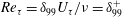
Results from the present rough wall experiments are compared, when possible, with the smooth wall measurements of Marusic et al. (Reference Marusic, Chauhan, Kulandaivelu and Hutchins2015), the rough wall data of Squire et al. (Reference Squire, Morrill-Winter, Hutchins, Schultz, Klewicki and Marusic2016) and the 2-D rough wall data of Krogstad & Efros (Reference Krogstad and Efros2012). The smooth wall measurements are performed using hot-wire anemometry in the large Melbourne boundary layer wind tunnel over a streamwise distance,
 $3.75\leqslant x\leqslant 18~\text{m}$
(Marusic et al.
Reference Marusic, Chauhan, Kulandaivelu and Hutchins2015). The Reynolds number at these measurement stations ranges between
$3.75\leqslant x\leqslant 18~\text{m}$
(Marusic et al.
Reference Marusic, Chauhan, Kulandaivelu and Hutchins2015). The Reynolds number at these measurement stations ranges between
 $3370\leqslant \unicode[STIX]{x1D6FF}_{99}^{+}\leqslant 9830$
. In all the smooth wall measurements, the friction velocity,
$3370\leqslant \unicode[STIX]{x1D6FF}_{99}^{+}\leqslant 9830$
. In all the smooth wall measurements, the friction velocity,
 $U_{\unicode[STIX]{x1D70F}}$
, is obtained by fitting the logarithmic mean velocity profile to the constants
$U_{\unicode[STIX]{x1D70F}}$
, is obtained by fitting the logarithmic mean velocity profile to the constants
 $\unicode[STIX]{x1D705}=0.384$
and
$\unicode[STIX]{x1D705}=0.384$
and
 $B=4.17$
(Chauhan, Nagib & Monkewitz Reference Chauhan, Nagib and Monkewitz2009). For the rough wall measurements of Squire et al. (Reference Squire, Morrill-Winter, Hutchins, Schultz, Klewicki and Marusic2016), only measurements at
$B=4.17$
(Chauhan, Nagib & Monkewitz Reference Chauhan, Nagib and Monkewitz2009). For the rough wall measurements of Squire et al. (Reference Squire, Morrill-Winter, Hutchins, Schultz, Klewicki and Marusic2016), only measurements at
 $x=21.7~\text{m}$
at different free-stream velocities are considered here. The primary reason for this is that Squire et al. (Reference Squire, Morrill-Winter, Hutchins, Schultz, Klewicki and Marusic2016) measured
$x=21.7~\text{m}$
at different free-stream velocities are considered here. The primary reason for this is that Squire et al. (Reference Squire, Morrill-Winter, Hutchins, Schultz, Klewicki and Marusic2016) measured
 $U_{\unicode[STIX]{x1D70F}}$
at this particular streamwise location using a large drag balance, as described in Baars et al. (Reference Baars, Squire, Talluru, Abbassi, Hutchins and Marusic2016). This enables us to compare our results with those of Squire et al. (Reference Squire, Morrill-Winter, Hutchins, Schultz, Klewicki and Marusic2016) without any ambiguity about
$U_{\unicode[STIX]{x1D70F}}$
at this particular streamwise location using a large drag balance, as described in Baars et al. (Reference Baars, Squire, Talluru, Abbassi, Hutchins and Marusic2016). This enables us to compare our results with those of Squire et al. (Reference Squire, Morrill-Winter, Hutchins, Schultz, Klewicki and Marusic2016) without any ambiguity about
 $U_{\unicode[STIX]{x1D70F}}$
. The 2-D rough wall measurements of Krogstad & Efros (Reference Krogstad and Efros2012) were made with using laser Doppler velocimetry (LDV) on a rough wall consisting of spanwise square bars (cross-section of 1.7 mm
$U_{\unicode[STIX]{x1D70F}}$
. The 2-D rough wall measurements of Krogstad & Efros (Reference Krogstad and Efros2012) were made with using laser Doppler velocimetry (LDV) on a rough wall consisting of spanwise square bars (cross-section of 1.7 mm
 $\times$
1.7 mm) arranged periodically with a spacing of
$\times$
1.7 mm) arranged periodically with a spacing of
 $p/k=8$
, similar to the present study. A floating element balance was used to determine
$p/k=8$
, similar to the present study. A floating element balance was used to determine
 $U_{\unicode[STIX]{x1D70F}}$
(see Krogstad & Efros Reference Krogstad and Efros2010, for full details). The Kármán Reynolds number (
$U_{\unicode[STIX]{x1D70F}}$
(see Krogstad & Efros Reference Krogstad and Efros2010, for full details). The Kármán Reynolds number (
 $\unicode[STIX]{x1D6FF}^{+}$
) at
$\unicode[STIX]{x1D6FF}^{+}$
) at
 $x=6.2~\text{m}$
on this rough wall is approximately 13 300 and
$x=6.2~\text{m}$
on this rough wall is approximately 13 300 and
 $k_{s}^{+}$
is approximately 320, suggesting that the flow is fully rough since
$k_{s}^{+}$
is approximately 320, suggesting that the flow is fully rough since
 $k_{s}^{+}\geqslant 100$
(Jiménez Reference Jiménez2004).
$k_{s}^{+}\geqslant 100$
(Jiménez Reference Jiménez2004).
2.1 Hot-wire anemometry
Hot-wire anemometry is used to measure streamwise velocity fluctuations. The single-wire probe is a Dantec 55P15 sensor; a
 $2.5~\unicode[STIX]{x03BC}\text{m}$
diameter Wollaston Pt -10%Rh wire is soldered between the prongs (separated by of 1.5 mm). The etched sensor length of the hot-wire is 0.5 mm giving a length to diameter ratio of 200, in keeping with the recommendations of Ligrani & Bradshaw (Reference Ligrani and Bradshaw1987) and Hutchins et al. (Reference Hutchins, Nickels, Marusic and Chong2009). The inner-normalised sensor length (
$2.5~\unicode[STIX]{x03BC}\text{m}$
diameter Wollaston Pt -10%Rh wire is soldered between the prongs (separated by of 1.5 mm). The etched sensor length of the hot-wire is 0.5 mm giving a length to diameter ratio of 200, in keeping with the recommendations of Ligrani & Bradshaw (Reference Ligrani and Bradshaw1987) and Hutchins et al. (Reference Hutchins, Nickels, Marusic and Chong2009). The inner-normalised sensor length (
 $l^{+}$
) in these experiments varied between 3.5 and 35.6. The single-wire probe is operated using an in-house constant temperature anemometer at an overheat ratio of 1.8. A
$l^{+}$
) in these experiments varied between 3.5 and 35.6. The single-wire probe is operated using an in-house constant temperature anemometer at an overheat ratio of 1.8. A
 $y$
-axis measuring device with a resolution of
$y$
-axis measuring device with a resolution of
 $1~\unicode[STIX]{x03BC}\text{m}$
is used in positioning the hot-wire probe close to the wall. The instrument comprises of a high magnification microscope 200
$1~\unicode[STIX]{x03BC}\text{m}$
is used in positioning the hot-wire probe close to the wall. The instrument comprises of a high magnification microscope 200
 $\times$
(Celestron digital microscope) mounted on a fine threaded traversing system. The measurement is accomplished using a digital indicator with a resolution of 0.001 mm. The indicator is set and zeroed on the top of the microscope and the displacement is recorded as the focusing is done from the wall to the hot-wire probe. A total of 36 logarithmically spaced measurement points between 0.2 and 136 mm are taken using the Mitutoyo height gauge with a resolution of 0.01 mm.
$\times$
(Celestron digital microscope) mounted on a fine threaded traversing system. The measurement is accomplished using a digital indicator with a resolution of 0.001 mm. The indicator is set and zeroed on the top of the microscope and the displacement is recorded as the focusing is done from the wall to the hot-wire probe. A total of 36 logarithmically spaced measurement points between 0.2 and 136 mm are taken using the Mitutoyo height gauge with a resolution of 0.01 mm.
A BAT-10 thermocouple (Physitemp) with a resolution of
 $0.1\,^{\circ }\text{C}$
was used to monitor the mean temperature in the free stream for the entire duration of the experiment. The hot-wire is calibrated in situ against the Pitot-static tube positioned in the undisturbed free-stream flow before and after every experiment at 16 different speeds ranging between
$0.1\,^{\circ }\text{C}$
was used to monitor the mean temperature in the free stream for the entire duration of the experiment. The hot-wire is calibrated in situ against the Pitot-static tube positioned in the undisturbed free-stream flow before and after every experiment at 16 different speeds ranging between
 $0$
and
$0$
and
 $22~\text{m}\,\text{s}^{-1}$
. A linear interpolation in time between pre- and post-calibrations (see Talluru et al.
Reference Talluru, Kulandaivelu, Hutchins and Marusic2014, for details) is used to account for any drift in the hot-wire voltage that occurs during the course of an experiment.
$22~\text{m}\,\text{s}^{-1}$
. A linear interpolation in time between pre- and post-calibrations (see Talluru et al.
Reference Talluru, Kulandaivelu, Hutchins and Marusic2014, for details) is used to account for any drift in the hot-wire voltage that occurs during the course of an experiment.
3 Results
3.1 Mean velocity

Figure 2. Present rough wall mean velocity profiles at several Reynolds numbers,
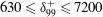 $630\leqslant \unicode[STIX]{x1D6FF}_{99}^{+}\leqslant 7200$
. See table 1 for symbols. The dot-dashed line represents the slope of the log region in a smooth wall turbulent boundary layer. Inset: variation of
$630\leqslant \unicode[STIX]{x1D6FF}_{99}^{+}\leqslant 7200$
. See table 1 for symbols. The dot-dashed line represents the slope of the log region in a smooth wall turbulent boundary layer. Inset: variation of
 $U_{\infty }^{+}$
with
$U_{\infty }^{+}$
with
 $\unicode[STIX]{x1D6FF}_{99}^{+}$
(open symbols represent the corresponding
$\unicode[STIX]{x1D6FF}_{99}^{+}$
(open symbols represent the corresponding
 $\unicode[STIX]{x1D6FF}^{+}$
values).
$\unicode[STIX]{x1D6FF}^{+}$
values).
Figure 2 shows mean velocity profiles normalised using inner scaling parameters, i.e.
 $U^{+}$
versus
$U^{+}$
versus
 $y^{+}$
, at a fixed
$y^{+}$
, at a fixed
 $x$
location as
$x$
location as
 $Re_{\unicode[STIX]{x1D70F}}=\unicode[STIX]{x1D6FF}_{99}^{+}$
increases from 630 to 7200. It is clearly evident that the mean velocity profile shifts downward and towards larger
$Re_{\unicode[STIX]{x1D70F}}=\unicode[STIX]{x1D6FF}_{99}^{+}$
increases from 630 to 7200. It is clearly evident that the mean velocity profile shifts downward and towards larger
 $y^{+}$
as
$y^{+}$
as
 $Re_{\unicode[STIX]{x1D70F}}$
increases, which is due to
$Re_{\unicode[STIX]{x1D70F}}$
increases, which is due to
 $U_{\unicode[STIX]{x1D70F}}$
increasing with
$U_{\unicode[STIX]{x1D70F}}$
increasing with
 $Re_{\unicode[STIX]{x1D70F}}$
. However, the rate of the downward shift decreases and eventually becomes zero, i.e. the mean velocity profile ceases to move downwards once
$Re_{\unicode[STIX]{x1D70F}}$
. However, the rate of the downward shift decreases and eventually becomes zero, i.e. the mean velocity profile ceases to move downwards once
 $Re_{\unicode[STIX]{x1D70F}}$
reaches a value of approximately 4000. Beyond this value, the profile simply shifts to larger
$Re_{\unicode[STIX]{x1D70F}}$
reaches a value of approximately 4000. Beyond this value, the profile simply shifts to larger
 $y^{+}$
, while its shape remains unchanged. The inset plot in figure 2 shows the variation of
$y^{+}$
, while its shape remains unchanged. The inset plot in figure 2 shows the variation of
 $U_{\infty }^{+}$
as a function of
$U_{\infty }^{+}$
as a function of
 $Re_{\unicode[STIX]{x1D70F}}$
(or
$Re_{\unicode[STIX]{x1D70F}}$
(or
 $\unicode[STIX]{x1D6FF}_{99}^{+}$
). The trend is clear: as
$\unicode[STIX]{x1D6FF}_{99}^{+}$
). The trend is clear: as
 $Re_{\unicode[STIX]{x1D70F}}$
increases,
$Re_{\unicode[STIX]{x1D70F}}$
increases,
 $U_{\infty }^{+}(\equiv [\sqrt{C_{f}/2}]^{-1})$
first decreases before reaching a constant value for
$U_{\infty }^{+}(\equiv [\sqrt{C_{f}/2}]^{-1})$
first decreases before reaching a constant value for
 $Re_{\unicode[STIX]{x1D70F}}\geqslant 4000$
. This indicates that the downward shift ceases at the same time as the coefficient of friction becomes constant and the TBL can be considered fully rough; in this fully rough regime, the drag is solely made of the form drag of the roughness elements. The continuous shift of the entire profile to larger values of
$Re_{\unicode[STIX]{x1D70F}}\geqslant 4000$
. This indicates that the downward shift ceases at the same time as the coefficient of friction becomes constant and the TBL can be considered fully rough; in this fully rough regime, the drag is solely made of the form drag of the roughness elements. The continuous shift of the entire profile to larger values of
 $y^{+}$
suggests that the length scale
$y^{+}$
suggests that the length scale
 $\unicode[STIX]{x1D708}/U_{\unicode[STIX]{x1D70F}}$
is not an appropriate length scale. The profile continues to shift horizontally because
$\unicode[STIX]{x1D708}/U_{\unicode[STIX]{x1D70F}}$
is not an appropriate length scale. The profile continues to shift horizontally because
 $U_{\unicode[STIX]{x1D70F}}$
increases with
$U_{\unicode[STIX]{x1D70F}}$
increases with
 $Re_{\unicode[STIX]{x1D70F}}$
(see table 1), thus resulting in
$Re_{\unicode[STIX]{x1D70F}}$
(see table 1), thus resulting in
 $y^{+}$
increasing for a fixed value of
$y^{+}$
increasing for a fixed value of
 $y$
, but maintaining its shape.
$y$
, but maintaining its shape.
To verify the fixed form of the shape, we plot in figure 3 the three velocity profiles in figure 2 for which
 $U_{\infty }^{+}$
is constant as a function of
$U_{\infty }^{+}$
is constant as a function of
 $y/k$
. There is a clear collapse of the profiles across the entire boundary layer onto a single curve of the form:
$y/k$
. There is a clear collapse of the profiles across the entire boundary layer onto a single curve of the form:
 $$\begin{eqnarray}U^{+}=F(y/k),\end{eqnarray}$$
where
 $F$
is a function, which appears to be independent of Reynolds number. A similar behaviour (
$F$
is a function, which appears to be independent of Reynolds number. A similar behaviour (
 $U_{\infty }^{+}=\text{const}$
) can be observed in the sand-grain rough wall profiles of Squire et al. (Reference Squire, Morrill-Winter, Hutchins, Schultz, Klewicki and Marusic2016) (
$U_{\infty }^{+}=\text{const}$
) can be observed in the sand-grain rough wall profiles of Squire et al. (Reference Squire, Morrill-Winter, Hutchins, Schultz, Klewicki and Marusic2016) (
 $3970\leqslant Re_{\unicode[STIX]{x1D70F}}\leqslant 29\,900$
). However, it is achieved at a much higher
$3970\leqslant Re_{\unicode[STIX]{x1D70F}}\leqslant 29\,900$
). However, it is achieved at a much higher
 $Re_{\unicode[STIX]{x1D70F}}$
than in the present rough wall, illustrating the fact that a sand-grain rough wall TBL requires a larger
$Re_{\unicode[STIX]{x1D70F}}$
than in the present rough wall, illustrating the fact that a sand-grain rough wall TBL requires a larger
 $Re_{\unicode[STIX]{x1D70F}}$
than a 2-D rod rough wall TBL before it can become fully rough. For comparison, we also report in figure 3, the rough wall mean velocity profile of Krogstad & Efros (Reference Krogstad and Efros2012) (2-D transverse square bars with
$Re_{\unicode[STIX]{x1D70F}}$
than a 2-D rod rough wall TBL before it can become fully rough. For comparison, we also report in figure 3, the rough wall mean velocity profile of Krogstad & Efros (Reference Krogstad and Efros2012) (2-D transverse square bars with
 $p=8k$
). Considering that
$p=8k$
). Considering that
 $\unicode[STIX]{x1D6FF}^{+}=13\,300$
and
$\unicode[STIX]{x1D6FF}^{+}=13\,300$
and
 $k_{s}\simeq 325$
, one expects the profile to be in the fully rough regime. Despite the large difference in
$k_{s}\simeq 325$
, one expects the profile to be in the fully rough regime. Despite the large difference in
 $Re_{\unicode[STIX]{x1D70F}}$
between our data and those of Krogstad & Efros (Reference Krogstad and Efros2012), the latter profile is not too different from the present distributions, although its value of
$Re_{\unicode[STIX]{x1D70F}}$
between our data and those of Krogstad & Efros (Reference Krogstad and Efros2012), the latter profile is not too different from the present distributions, although its value of
 $U_{max}^{+}$
is slightly larger, reflecting a lower
$U_{max}^{+}$
is slightly larger, reflecting a lower
 $C_{f}$
in comparison to the present study;
$C_{f}$
in comparison to the present study;
 $C_{f}\simeq 0.0072$
, and 0.0068, for the present 2-D rough wall and that of Krogstad & Efros (Reference Krogstad and Efros2012), respectively.
$C_{f}\simeq 0.0072$
, and 0.0068, for the present 2-D rough wall and that of Krogstad & Efros (Reference Krogstad and Efros2012), respectively.

Figure 3. Mean velocity profiles in the present rough wall (black symbols) at several Reynolds numbers,
 $3940\leqslant Re_{\unicode[STIX]{x1D70F}}\leqslant 7200$
, sand-grain roughness (red symbols,
$3940\leqslant Re_{\unicode[STIX]{x1D70F}}\leqslant 7200$
, sand-grain roughness (red symbols,
 $Re_{\unicode[STIX]{x1D70F}}=20\,160$
, 25 020 and 29 900, Squire et al.
Reference Squire, Morrill-Winter, Hutchins, Schultz, Klewicki and Marusic2016) and square bar roughness (blue symbols,
$Re_{\unicode[STIX]{x1D70F}}=20\,160$
, 25 020 and 29 900, Squire et al.
Reference Squire, Morrill-Winter, Hutchins, Schultz, Klewicki and Marusic2016) and square bar roughness (blue symbols,
 $Re_{\unicode[STIX]{x1D70F}}=13\,300$
, Krogstad & Efros Reference Krogstad and Efros2012) as a function of
$Re_{\unicode[STIX]{x1D70F}}=13\,300$
, Krogstad & Efros Reference Krogstad and Efros2012) as a function of
 $y/k$
.
$y/k$
.
Figure 4 shows a clear collapse of the mean velocity profiles over the present rough wall, when plotted as a function of
 $y/\unicode[STIX]{x1D6FF}_{99}$
. The same trend is observed in the sand-grain roughness data of Squire et al. (Reference Squire, Morrill-Winter, Hutchins, Schultz, Klewicki and Marusic2016), however, the latter collapse onto a different curve. This difference is due to the difference in
$y/\unicode[STIX]{x1D6FF}_{99}$
. The same trend is observed in the sand-grain roughness data of Squire et al. (Reference Squire, Morrill-Winter, Hutchins, Schultz, Klewicki and Marusic2016), however, the latter collapse onto a different curve. This difference is due to the difference in
 $C_{f}$
between the two rough wall TBLs. It is well known that there is no such collapse for smooth wall TBL profiles because of
$C_{f}$
between the two rough wall TBLs. It is well known that there is no such collapse for smooth wall TBL profiles because of
 $Re_{\unicode[STIX]{x1D70F}}$
-dependence of
$Re_{\unicode[STIX]{x1D70F}}$
-dependence of
 $C_{f}$
. This is well illustrated in figure 4, where we plot the high Reynolds number smooth wall data of Marusic et al. (Reference Marusic, Chauhan, Kulandaivelu and Hutchins2015) (
$C_{f}$
. This is well illustrated in figure 4, where we plot the high Reynolds number smooth wall data of Marusic et al. (Reference Marusic, Chauhan, Kulandaivelu and Hutchins2015) (
 $3370\leqslant Re_{\unicode[STIX]{x1D70F}}\leqslant 9830$
) and the direct numerical simulation (DNS) data of Schlatter & Örlü (Reference Schlatter and Örlü2010) (
$3370\leqslant Re_{\unicode[STIX]{x1D70F}}\leqslant 9830$
) and the direct numerical simulation (DNS) data of Schlatter & Örlü (Reference Schlatter and Örlü2010) (
 $Re_{\unicode[STIX]{x1D70F}}=674$
). Of particular interest, is the rough wall velocity profile of Krogstad & Efros (Reference Krogstad and Efros2012), also reported in the figure for comparison. This profile collapses relatively well onto the present 2-D rough wall profiles, as it could have been anticipated from figure 3 and the similar values of
$Re_{\unicode[STIX]{x1D70F}}=674$
). Of particular interest, is the rough wall velocity profile of Krogstad & Efros (Reference Krogstad and Efros2012), also reported in the figure for comparison. This profile collapses relatively well onto the present 2-D rough wall profiles, as it could have been anticipated from figure 3 and the similar values of
 $C_{f}$
, suggesting that both TBLs share similarities. This may not be too surprising considering the rough walls share almost the same roughness geometry, cylindrical rods and square bars with the same
$C_{f}$
, suggesting that both TBLs share similarities. This may not be too surprising considering the rough walls share almost the same roughness geometry, cylindrical rods and square bars with the same
 $k$
and
$k$
and
 $p$
, although
$p$
, although
 $\unicode[STIX]{x1D6FF}/k$
for the square bar rough wall is approximately twice the present value.
$\unicode[STIX]{x1D6FF}/k$
for the square bar rough wall is approximately twice the present value.

Figure 4. Mean velocity profiles over the present 2-D rough wall (back symbols) as a function of
 $y/\unicode[STIX]{x1D6FF}$
. Symbols as in table 1. Red symbols: (Squire et al.
Reference Squire, Morrill-Winter, Hutchins, Schultz, Klewicki and Marusic2016,
$y/\unicode[STIX]{x1D6FF}$
. Symbols as in table 1. Red symbols: (Squire et al.
Reference Squire, Morrill-Winter, Hutchins, Schultz, Klewicki and Marusic2016,
 $Re_{\unicode[STIX]{x1D70F}}=20\,160$
, 25 020, and 29 900); blue symbols: (Krogstad & Efros Reference Krogstad and Efros2012,
$Re_{\unicode[STIX]{x1D70F}}=20\,160$
, 25 020, and 29 900); blue symbols: (Krogstad & Efros Reference Krogstad and Efros2012,
 $Re_{\unicode[STIX]{x1D70F}}=13\,300$
); dashed lines: smooth wall data (Marusic et al.
Reference Marusic, Chauhan, Kulandaivelu and Hutchins2015,
$Re_{\unicode[STIX]{x1D70F}}=13\,300$
); dashed lines: smooth wall data (Marusic et al.
Reference Marusic, Chauhan, Kulandaivelu and Hutchins2015,
 $Re_{\unicode[STIX]{x1D70F}}=3370$
, 4760, 6450 and 9830) and solid line: smooth wall DNS data (Schlatter & Örlü Reference Schlatter and Örlü2010,
$Re_{\unicode[STIX]{x1D70F}}=3370$
, 4760, 6450 and 9830) and solid line: smooth wall DNS data (Schlatter & Örlü Reference Schlatter and Örlü2010,
 $Re_{\unicode[STIX]{x1D70F}}=674$
). Only the profiles for which
$Re_{\unicode[STIX]{x1D70F}}=674$
). Only the profiles for which
 $U_{\infty }/U_{\unicode[STIX]{x1D70F}}$
is constant in the present rough wall and sand-grain roughness (Squire et al.
Reference Squire, Morrill-Winter, Hutchins, Schultz, Klewicki and Marusic2016) TBLs are shown.
$U_{\infty }/U_{\unicode[STIX]{x1D70F}}$
is constant in the present rough wall and sand-grain roughness (Squire et al.
Reference Squire, Morrill-Winter, Hutchins, Schultz, Klewicki and Marusic2016) TBLs are shown.
Altogether, the results presented in figures 2–4 are consistent with a
 $Re$
independence of the normalised mean velocity profile, which would suggest that the Reynolds number similarity is well achieved in a rough wall TBL, at least in the context of the mean velocity. Note that unlike a smooth wall TBL, where one must exclude the viscous-dominated near-wall region if such similarity is to be observed, the Reynolds number similarity is observed across practically the entire boundary layer for a fully rough TBL. This is possible because the spatially averaged viscosity effects in the near-wall region are either zero or negligible. The sand-grain rough wall data of Squire et al. (Reference Squire, Morrill-Winter, Hutchins, Schultz, Klewicki and Marusic2016) also show that when
$Re$
independence of the normalised mean velocity profile, which would suggest that the Reynolds number similarity is well achieved in a rough wall TBL, at least in the context of the mean velocity. Note that unlike a smooth wall TBL, where one must exclude the viscous-dominated near-wall region if such similarity is to be observed, the Reynolds number similarity is observed across practically the entire boundary layer for a fully rough TBL. This is possible because the spatially averaged viscosity effects in the near-wall region are either zero or negligible. The sand-grain rough wall data of Squire et al. (Reference Squire, Morrill-Winter, Hutchins, Schultz, Klewicki and Marusic2016) also show that when
 $Re$
is large enough the normalised velocity profiles collapse onto a single distribution. However, that distribution differs from that of the present data due to a difference in the value of the form drag coefficient. To illustrate this, we employ the so-called diagnostic plot (Alfredsson Reference Alfredsson and Örlü2010; Alfredsson, Segalini & Örlü Reference Alfredsson, Segalini and Örlü2011; Örlü et al.
Reference Örlü, Segalini, Klewicki and Alfredsson2016), which consists of plotting
$Re$
is large enough the normalised velocity profiles collapse onto a single distribution. However, that distribution differs from that of the present data due to a difference in the value of the form drag coefficient. To illustrate this, we employ the so-called diagnostic plot (Alfredsson Reference Alfredsson and Örlü2010; Alfredsson, Segalini & Örlü Reference Alfredsson, Segalini and Örlü2011; Örlü et al.
Reference Örlü, Segalini, Klewicki and Alfredsson2016), which consists of plotting
 $u^{\prime }$
as a function of
$u^{\prime }$
as a function of
 $U$
, thus removing any ambiguity associated with knowing
$U$
, thus removing any ambiguity associated with knowing
 $y$
and
$y$
and
 $U_{\unicode[STIX]{x1D70F}}$
accurately. Figure 5 shows such plots, where
$U_{\unicode[STIX]{x1D70F}}$
accurately. Figure 5 shows such plots, where
 $u^{\prime }$
and
$u^{\prime }$
and
 $U$
are normalised by
$U$
are normalised by
 $U$
and
$U$
and
 $U_{\infty }$
, respectively. While for each surface there is a clear collapse of the distributions across the entire boundary layer, the collapse is different between the two surfaces, in conformity with two distinct drag coefficients (
$U_{\infty }$
, respectively. While for each surface there is a clear collapse of the distributions across the entire boundary layer, the collapse is different between the two surfaces, in conformity with two distinct drag coefficients (
 $C_{f}\simeq$
0.0072 and 0.0032 for the present data and the sand-grain roughness, respectively). Further, the trend shown by the data indicates that the distributions for the two rough walls will remain distinct, regardless of the Reynolds number, hence suggesting two distinct
$C_{f}\simeq$
0.0072 and 0.0032 for the present data and the sand-grain roughness, respectively). Further, the trend shown by the data indicates that the distributions for the two rough walls will remain distinct, regardless of the Reynolds number, hence suggesting two distinct
 $Re$
-independent profiles. It appears thus that a
$Re$
-independent profiles. It appears thus that a
 $Re$
-independent normalised mean velocity profile for the complete TBL is possible for fully rough wall TBLs. However, the profile cannot be universal since it is controlled by the rough wall drag coefficient which varies between roughness geometries as evidenced in figure 4.
$Re$
-independent normalised mean velocity profile for the complete TBL is possible for fully rough wall TBLs. However, the profile cannot be universal since it is controlled by the rough wall drag coefficient which varies between roughness geometries as evidenced in figure 4.

Figure 5. Diagnostic plot for the present rough wall (black symbols), sand-grain roughness (red symbols,
 $Re_{\unicode[STIX]{x1D70F}}=20\,160$
, 25 020, and 29 900, Squire et al.
Reference Squire, Morrill-Winter, Hutchins, Schultz, Klewicki and Marusic2016) and the square bar roughness (blue symbols,
$Re_{\unicode[STIX]{x1D70F}}=20\,160$
, 25 020, and 29 900, Squire et al.
Reference Squire, Morrill-Winter, Hutchins, Schultz, Klewicki and Marusic2016) and the square bar roughness (blue symbols,
 $Re_{\unicode[STIX]{x1D70F}}=13\,300$
, Krogstad & Efros Reference Krogstad and Efros2012).
$Re_{\unicode[STIX]{x1D70F}}=13\,300$
, Krogstad & Efros Reference Krogstad and Efros2012).
Another parameter that is also likely to control the
 $Re$
-independent profile of a rough wall TBL, for a given roughness geometry, is the ratio
$Re$
-independent profile of a rough wall TBL, for a given roughness geometry, is the ratio
 $\unicode[STIX]{x1D6FF}/k$
. It is expected that for a given roughness geometry,
$\unicode[STIX]{x1D6FF}/k$
. It is expected that for a given roughness geometry,
 $C_{f}$
will change with
$C_{f}$
will change with
 $\unicode[STIX]{x1D6FF}/k$
;
$\unicode[STIX]{x1D6FF}/k$
;
 $\unicode[STIX]{x1D6FF}/k=63$
and 200 for the present profiles and those of Squire et al. (Reference Squire, Morrill-Winter, Hutchins, Schultz, Klewicki and Marusic2016), respectively, shown in figures 4 and 5. This raises the following question: can the
$\unicode[STIX]{x1D6FF}/k=63$
and 200 for the present profiles and those of Squire et al. (Reference Squire, Morrill-Winter, Hutchins, Schultz, Klewicki and Marusic2016), respectively, shown in figures 4 and 5. This raises the following question: can the
 $Re$
-independent profiles for both rough walls collapse if one varies
$Re$
-independent profiles for both rough walls collapse if one varies
 $\unicode[STIX]{x1D6FF}/k$
? (Such collapse would result in both rough walls yielding the same diagnostic distribution.) The above results show that simply invoking Townsend’s Reynolds number similarity to address the question is not enough. The answer requires one to carry out a series of parametric measurements for both rough wall TBLs in the fully rough regime by systematically changing the value of
$\unicode[STIX]{x1D6FF}/k$
? (Such collapse would result in both rough walls yielding the same diagnostic distribution.) The above results show that simply invoking Townsend’s Reynolds number similarity to address the question is not enough. The answer requires one to carry out a series of parametric measurements for both rough wall TBLs in the fully rough regime by systematically changing the value of
 $\unicode[STIX]{x1D6FF}/k$
. However, one expects to observe the same result as presented here. Indeed, consider for example the 2-D rough wall where one changes
$\unicode[STIX]{x1D6FF}/k$
. However, one expects to observe the same result as presented here. Indeed, consider for example the 2-D rough wall where one changes
 $k$
, while maintaining
$k$
, while maintaining
 $p/k$
constant and equal to 8. Regardless of
$p/k$
constant and equal to 8. Regardless of
 $k$
and as long as
$k$
and as long as
 $\unicode[STIX]{x1D6FF}/k$
is large enough (at least larger than 40 (Jiménez Reference Jiménez2004)), the fully rough regime will yield the same
$\unicode[STIX]{x1D6FF}/k$
is large enough (at least larger than 40 (Jiménez Reference Jiménez2004)), the fully rough regime will yield the same
 $C_{f}$
as for the present case, and thus the same normalised velocity profiles as shown in figure 2 will be obtained. This appears to be confirmed by the data of Krogstad & Efros (Reference Krogstad and Efros2012) reported in figure 5. Despite the difference in the cross-sectional shape between the present roughness and that of Krogstad & Efros (Reference Krogstad and Efros2012) (circular rods versus square bars), the distributions are practically identical. Of course, the critical
$C_{f}$
as for the present case, and thus the same normalised velocity profiles as shown in figure 2 will be obtained. This appears to be confirmed by the data of Krogstad & Efros (Reference Krogstad and Efros2012) reported in figure 5. Despite the difference in the cross-sectional shape between the present roughness and that of Krogstad & Efros (Reference Krogstad and Efros2012) (circular rods versus square bars), the distributions are practically identical. Of course, the critical
 $Re$
at which the fully rough regime will be achieved will vary with
$Re$
at which the fully rough regime will be achieved will vary with
 $k$
. This implies that two distinct roughness geometries, as for example in the present work, will lead to two distinct
$k$
. This implies that two distinct roughness geometries, as for example in the present work, will lead to two distinct
 $Re$
-independent normalised mean velocity profiles in the fully rough regime. These differences can be further elucidated by comparing the turbulence intensity profiles in the outer region of the smooth and rough wall TBLs based on a modified diagnostic plot proposed by Castro, Segalini & Alfredsson (Reference Castro, Segalini and Alfredsson2013) and reported in figure 6. This modified diagnostic plot produces a better collapse of all curves than the original one. It seems that by introducing the velocity deficit (
$Re$
-independent normalised mean velocity profiles in the fully rough regime. These differences can be further elucidated by comparing the turbulence intensity profiles in the outer region of the smooth and rough wall TBLs based on a modified diagnostic plot proposed by Castro, Segalini & Alfredsson (Reference Castro, Segalini and Alfredsson2013) and reported in figure 6. This modified diagnostic plot produces a better collapse of all curves than the original one. It seems that by introducing the velocity deficit (
 $\unicode[STIX]{x0394}U$
), the difference between smooth, and different types of rough walls is dramatically reduced. Note though that the collapse is not perfect. While the non-collapse for
$\unicode[STIX]{x0394}U$
), the difference between smooth, and different types of rough walls is dramatically reduced. Note though that the collapse is not perfect. While the non-collapse for
 $U^{\prime }/U_{\infty }^{\prime }\leqslant 0.7$
can be explained in terms of the differences in turbulence levels in the near-wall region of different types of TBLs, the reason for the variation in the region
$U^{\prime }/U_{\infty }^{\prime }\leqslant 0.7$
can be explained in terms of the differences in turbulence levels in the near-wall region of different types of TBLs, the reason for the variation in the region
 $U^{\prime }/U_{\infty }^{\prime }\geqslant 0.8$
between the 2-D bars and the sand-grain roughness is not clear; this may reflect a real difference associated with the roughness geometry or the possibility that the sand-grain paper data of Squire et al. (Reference Squire, Morrill-Winter, Hutchins, Schultz, Klewicki and Marusic2016) are not fully rough (albeit
$U^{\prime }/U_{\infty }^{\prime }\geqslant 0.8$
between the 2-D bars and the sand-grain roughness is not clear; this may reflect a real difference associated with the roughness geometry or the possibility that the sand-grain paper data of Squire et al. (Reference Squire, Morrill-Winter, Hutchins, Schultz, Klewicki and Marusic2016) are not fully rough (albeit
 $C_{f}$
appears to be constant in the experimental data of Squire et al. (Reference Squire, Morrill-Winter, Hutchins, Schultz, Klewicki and Marusic2016)).
$C_{f}$
appears to be constant in the experimental data of Squire et al. (Reference Squire, Morrill-Winter, Hutchins, Schultz, Klewicki and Marusic2016)).

Figure 6. Comparison of turbulence intensities in the outer layer of smooth (dotted line,
 $Re_{\unicode[STIX]{x1D70F}}=9830$
, Marusic et al.
Reference Marusic, Chauhan, Kulandaivelu and Hutchins2015) and rough wall turbulent boundary layers (data from figure 5) using the modified diagnostic plot (Castro et al.
Reference Castro, Segalini and Alfredsson2013). Here,
$Re_{\unicode[STIX]{x1D70F}}=9830$
, Marusic et al.
Reference Marusic, Chauhan, Kulandaivelu and Hutchins2015) and rough wall turbulent boundary layers (data from figure 5) using the modified diagnostic plot (Castro et al.
Reference Castro, Segalini and Alfredsson2013). Here,
 $U^{\prime }=U+\unicode[STIX]{x0394}U$
and
$U^{\prime }=U+\unicode[STIX]{x0394}U$
and
 $U_{\infty }^{\prime }=U_{\infty }+\unicode[STIX]{x0394}U$
and
$U_{\infty }^{\prime }=U_{\infty }+\unicode[STIX]{x0394}U$
and
 $\unicode[STIX]{x0394}U$
is the velocity defect. The solid line is the smooth wall outer layer straight line from Alfredsson, Örlü & Segalini (Reference Alfredsson, Örlü and Segalini2012).
$\unicode[STIX]{x0394}U$
is the velocity defect. The solid line is the smooth wall outer layer straight line from Alfredsson, Örlü & Segalini (Reference Alfredsson, Örlü and Segalini2012).

Figure 7. Comparison of velocity defect profiles in smooth wall (black dashed lines,
 $Re_{\unicode[STIX]{x1D70F}}=3370$
, 4760, 6450 and 9830, Marusic et al.
Reference Marusic, Chauhan, Kulandaivelu and Hutchins2015), sand-grain roughness (red symbols,
$Re_{\unicode[STIX]{x1D70F}}=3370$
, 4760, 6450 and 9830, Marusic et al.
Reference Marusic, Chauhan, Kulandaivelu and Hutchins2015), sand-grain roughness (red symbols,
 $Re_{\unicode[STIX]{x1D70F}}=20\,160$
, 25 020 and 29 900, Squire et al.
Reference Squire, Morrill-Winter, Hutchins, Schultz, Klewicki and Marusic2016), square bar (blue symbols,
$Re_{\unicode[STIX]{x1D70F}}=20\,160$
, 25 020 and 29 900, Squire et al.
Reference Squire, Morrill-Winter, Hutchins, Schultz, Klewicki and Marusic2016), square bar (blue symbols,
 $Re_{\unicode[STIX]{x1D70F}}=13\,300$
, Krogstad & Efros Reference Krogstad and Efros2012) and the present rough wall data (black symbols) normalised by (a)
$Re_{\unicode[STIX]{x1D70F}}=13\,300$
, Krogstad & Efros Reference Krogstad and Efros2012) and the present rough wall data (black symbols) normalised by (a)
 $U_{\unicode[STIX]{x1D70F}}$
and (b)
$U_{\unicode[STIX]{x1D70F}}$
and (b)
 $U_{\infty }$
. Refer to caption of figure 4 for symbols used for smooth wall, sand-grain and square bar rough wall TBLs.
$U_{\infty }$
. Refer to caption of figure 4 for symbols used for smooth wall, sand-grain and square bar rough wall TBLs.
It is common to test the universality of TBL velocity profiles by plotting the velocity profiles in the deficit form, (Townsend Reference Townsend1956):
 $$\begin{eqnarray}\frac{U_{\infty }-U}{u_{o}}=f(y/\unicode[STIX]{x1D702}),\end{eqnarray}$$
where
 $u_{o}$
and
$u_{o}$
and
 $\unicode[STIX]{x1D702}$
are velocity and length scales, respectively, and have been the subject of many investigations (i.e. Townsend (Reference Townsend1976), George & Castillo (Reference George and Castillo1997), Zagarola & Smits (Reference Zagarola and Smits1998), Jones, Nickels & Marusic (Reference Jones, Nickels and Marusic2008), Talluru et al. (Reference Talluru, Djenidi, Kamruzzaman and Antonia2016)). Here, we use
$\unicode[STIX]{x1D702}$
are velocity and length scales, respectively, and have been the subject of many investigations (i.e. Townsend (Reference Townsend1976), George & Castillo (Reference George and Castillo1997), Zagarola & Smits (Reference Zagarola and Smits1998), Jones, Nickels & Marusic (Reference Jones, Nickels and Marusic2008), Talluru et al. (Reference Talluru, Djenidi, Kamruzzaman and Antonia2016)). Here, we use
 $U_{\unicode[STIX]{x1D70F}}$
,
$U_{\unicode[STIX]{x1D70F}}$
,
 $U_{\infty }$
and
$U_{\infty }$
and
 $\unicode[STIX]{x1D6FF}$
because Talluru et al. (Reference Talluru, Djenidi, Kamruzzaman and Antonia2016) showed that these are correct scaling variables for rough wall TBLs (use of the length scale
$\unicode[STIX]{x1D6FF}$
because Talluru et al. (Reference Talluru, Djenidi, Kamruzzaman and Antonia2016) showed that these are correct scaling variables for rough wall TBLs (use of the length scale
 $\unicode[STIX]{x1D6FF}^{\ast }[2/C_{f}]^{1/2}$
(Rotta Reference Rotta1962), where
$\unicode[STIX]{x1D6FF}^{\ast }[2/C_{f}]^{1/2}$
(Rotta Reference Rotta1962), where
 $\unicode[STIX]{x1D6FF}^{\ast }$
is the displacement thickness, does not change the results). Figure 7(a,b) shows the velocity defect profiles for the rough wall data and the same smooth wall data as reported in figure 4 normalised by
$\unicode[STIX]{x1D6FF}^{\ast }$
is the displacement thickness, does not change the results). Figure 7(a,b) shows the velocity defect profiles for the rough wall data and the same smooth wall data as reported in figure 4 normalised by
 $U_{\unicode[STIX]{x1D70F}}$
and
$U_{\unicode[STIX]{x1D70F}}$
and
 $U_{\infty }$
, respectively. Universality is thought to be reflected in the collapse of the normalised velocity defect profiles. For the rough wall data, the use of either
$U_{\infty }$
, respectively. Universality is thought to be reflected in the collapse of the normalised velocity defect profiles. For the rough wall data, the use of either
 $U_{\unicode[STIX]{x1D70F}}$
or
$U_{\unicode[STIX]{x1D70F}}$
or
 $U_{\infty }$
as a scaling velocity results in a good collapse. In particular, the collapse is perfect for the profiles for which
$U_{\infty }$
as a scaling velocity results in a good collapse. In particular, the collapse is perfect for the profiles for which
 $U_{\infty }^{+}$
is constant, confirming that a
$U_{\infty }^{+}$
is constant, confirming that a
 $Re$
-independent normalised velocity distribution is achieved. The smooth wall data present an interesting paradox: the velocity defect profiles collapse when normalised with
$Re$
-independent normalised velocity distribution is achieved. The smooth wall data present an interesting paradox: the velocity defect profiles collapse when normalised with
 $U_{\unicode[STIX]{x1D70F}}$
, but not when normalised with
$U_{\unicode[STIX]{x1D70F}}$
, but not when normalised with
 $U_{\infty }$
. In order to solve this paradox we write the left-hand side of (3.2) as follows,
$U_{\infty }$
. In order to solve this paradox we write the left-hand side of (3.2) as follows,
 $$\begin{eqnarray}\frac{U_{\infty }-U}{U_{\unicode[STIX]{x1D70F}}}=\left[\frac{2}{C_{f}}\right]^{1/2}\left(\frac{U_{\infty }-U}{U_{\infty }}\right).\end{eqnarray}$$
For the smooth wall,
 $C_{f}$
is function of
$C_{f}$
is function of
 $Re$
;
$Re$
;
 $C_{f}$
decreases with increasing
$C_{f}$
decreases with increasing
 $Re$
, thus compensating for the
$Re$
, thus compensating for the
 $Re$
dependence of
$Re$
dependence of
 $(U_{\infty }-U)/U_{\infty }$
which leads to the collapse of the profiles. We note though that they collapse relatively well with the rough wall profiles when normalised with
$(U_{\infty }-U)/U_{\infty }$
which leads to the collapse of the profiles. We note though that they collapse relatively well with the rough wall profiles when normalised with
 $U_{\unicode[STIX]{x1D70F}}$
. The collapse of
$U_{\unicode[STIX]{x1D70F}}$
. The collapse of
 $(U_{\infty }-U)/U_{\unicode[STIX]{x1D70F}}$
between the rough wall and the smooth wall data is often used to demonstrate the universality of the velocity profiles in TBLs and validate Townsend’s Reynolds number similarity. Interestingly, Townsend (Reference Townsend1956) states that ‘if, as must be assumed, Reynolds number similarity of self-preserving flow exists, the form of the self-preserving functions is universal for any one type of flow’. This implies that
$(U_{\infty }-U)/U_{\unicode[STIX]{x1D70F}}$
between the rough wall and the smooth wall data is often used to demonstrate the universality of the velocity profiles in TBLs and validate Townsend’s Reynolds number similarity. Interestingly, Townsend (Reference Townsend1956) states that ‘if, as must be assumed, Reynolds number similarity of self-preserving flow exists, the form of the self-preserving functions is universal for any one type of flow’. This implies that
 $(U_{\infty }-U)/U_{\unicode[STIX]{x1D70F}}$
and
$(U_{\infty }-U)/U_{\unicode[STIX]{x1D70F}}$
and
 $(U_{\infty }-U)/U_{\infty }$
must be similar in form for any
$(U_{\infty }-U)/U_{\infty }$
must be similar in form for any
 $Re$
, if both
$Re$
, if both
 $U_{\unicode[STIX]{x1D70F}}$
and
$U_{\unicode[STIX]{x1D70F}}$
and
 $U_{\infty }$
are proper scaling velocities compliant with self-preservation analysis (Talluru et al.
Reference Talluru, Djenidi, Kamruzzaman and Antonia2016).
$U_{\infty }$
are proper scaling velocities compliant with self-preservation analysis (Talluru et al.
Reference Talluru, Djenidi, Kamruzzaman and Antonia2016).
For the rough wall,
 $C_{f}$
is constant in the fully rough regime. Thus, using either
$C_{f}$
is constant in the fully rough regime. Thus, using either
 $U_{\unicode[STIX]{x1D70F}}$
or
$U_{\unicode[STIX]{x1D70F}}$
or
 $U_{\infty }$
leads to the same collapse which is consistent with the Reynolds number similarity. The data of Squire et al. (Reference Squire, Morrill-Winter, Hutchins, Schultz, Klewicki and Marusic2016) show the same result. Regardless of the choice of
$U_{\infty }$
leads to the same collapse which is consistent with the Reynolds number similarity. The data of Squire et al. (Reference Squire, Morrill-Winter, Hutchins, Schultz, Klewicki and Marusic2016) show the same result. Regardless of the choice of
 $u_{o}$
, the normalised velocity defect profiles collapse. However, while the sand-grain rough wall data collapse with the present velocity defect profiles when normalised by
$u_{o}$
, the normalised velocity defect profiles collapse. However, while the sand-grain rough wall data collapse with the present velocity defect profiles when normalised by
 $U_{\unicode[STIX]{x1D70F}}$
, they collapse onto a different curve than the present rough wall one when normalised by
$U_{\unicode[STIX]{x1D70F}}$
, they collapse onto a different curve than the present rough wall one when normalised by
 $U_{\infty }$
. The data of Krogstad & Efros (Reference Krogstad and Efros2012) differ slightly from the present data when normalised by
$U_{\infty }$
. The data of Krogstad & Efros (Reference Krogstad and Efros2012) differ slightly from the present data when normalised by
 $U_{\infty }$
, certainly reflecting the slightly smaller value of
$U_{\infty }$
, certainly reflecting the slightly smaller value of
 $C_{f}$
.
$C_{f}$
.
For the smooth wall, equation (3.3) indicates that
 $(U_{\infty }-U)/U_{\unicode[STIX]{x1D70F}}$
and
$(U_{\infty }-U)/U_{\unicode[STIX]{x1D70F}}$
and
 $(U_{\infty }-U)/U_{\infty }$
cannot both be
$(U_{\infty }-U)/U_{\infty }$
cannot both be
 $Re$
-independent, as shown in figure 7(a,b), since
$Re$
-independent, as shown in figure 7(a,b), since
 $C_{f}$
is
$C_{f}$
is
 $Re$
-dependent. George & Castillo (Reference George and Castillo1997) argued, based on the asymptotic invariance principle, that the velocity deficit in the outer layer scales as
$Re$
-dependent. George & Castillo (Reference George and Castillo1997) argued, based on the asymptotic invariance principle, that the velocity deficit in the outer layer scales as
 $(U_{\infty }-U)/U_{\infty }$
in the
$(U_{\infty }-U)/U_{\infty }$
in the
 $Re$
-independent regime. Note that even if the smooth wall profiles
$Re$
-independent regime. Note that even if the smooth wall profiles
 $(U_{\infty }-U)/U_{\infty }$
collapse (in the outer part of the layer); figure 7(b) shows that they will certainly collapse onto a different curve than that for the rough walls. Notice how the trend shown by the distributions altogether in figure 7(b) reflects that of the profiles in figure 4; as the distributions in figure 4 shift downwards, they shift upwards in figure 7(b). This can be explained if we write
$(U_{\infty }-U)/U_{\infty }$
collapse (in the outer part of the layer); figure 7(b) shows that they will certainly collapse onto a different curve than that for the rough walls. Notice how the trend shown by the distributions altogether in figure 7(b) reflects that of the profiles in figure 4; as the distributions in figure 4 shift downwards, they shift upwards in figure 7(b). This can be explained if we write
 $1-U/U_{\infty }=1-(U/U_{\unicode[STIX]{x1D70F}})(C_{f}/2)^{1/2}$
. It appears then that
$1-U/U_{\infty }=1-(U/U_{\unicode[STIX]{x1D70F}})(C_{f}/2)^{1/2}$
. It appears then that
 $(U/U_{\unicode[STIX]{x1D70F}})(C_{f}/2)^{1/2}$
is larger for a smooth wall TBL than a rough wall TBL; further, while it is constant (i.e. independent of
$(U/U_{\unicode[STIX]{x1D70F}})(C_{f}/2)^{1/2}$
is larger for a smooth wall TBL than a rough wall TBL; further, while it is constant (i.e. independent of
 $Re$
) for a given fully rough wall TBL, it increases with
$Re$
) for a given fully rough wall TBL, it increases with
 $Re$
for a smooth wall TBL. This result shows that the distribution (
$Re$
for a smooth wall TBL. This result shows that the distribution (
 $1-U/U_{\infty }$
) or simply (
$1-U/U_{\infty }$
) or simply (
 $U/U_{\infty }$
) should be used for assessing a
$U/U_{\infty }$
) should be used for assessing a
 $Re$
-independence state. Indeed, when such state is reached, the profiles,
$Re$
-independence state. Indeed, when such state is reached, the profiles,
 $U/U_{\infty }$
, must collapse onto a single curve; this curve varies with the roughness geometry or the coefficient of drag.
$U/U_{\infty }$
, must collapse onto a single curve; this curve varies with the roughness geometry or the coefficient of drag.
It is remarkable that while the profiles
 $(U_{\infty }-U)/U_{\infty }$
differ between smooth and rough walls, the profiles for
$(U_{\infty }-U)/U_{\infty }$
differ between smooth and rough walls, the profiles for
 $(U_{\infty }-U)/U_{\unicode[STIX]{x1D70F}}$
collapse relatively well onto each other. We saw above that the compensational effect of
$(U_{\infty }-U)/U_{\unicode[STIX]{x1D70F}}$
collapse relatively well onto each other. We saw above that the compensational effect of
 $C_{f}$
on
$C_{f}$
on
 $(U_{\infty }-U)/U_{\infty }$
leads to a collapse of the profiles
$(U_{\infty }-U)/U_{\infty }$
leads to a collapse of the profiles
 $(U_{\infty }-U)/U_{\unicode[STIX]{x1D70F}}$
for the smooth wall. However, the collapse of
$(U_{\infty }-U)/U_{\unicode[STIX]{x1D70F}}$
for the smooth wall. However, the collapse of
 $(U_{\infty }-U)/U_{\unicode[STIX]{x1D70F}}$
between the rough and smooth wall data may not in fact be too surprising. To see this, let us first note that the downward shift of the rough wall mean velocity profiles,
$(U_{\infty }-U)/U_{\unicode[STIX]{x1D70F}}$
between the rough and smooth wall data may not in fact be too surprising. To see this, let us first note that the downward shift of the rough wall mean velocity profiles,
 $\unicode[STIX]{x0394}U^{+}$
, can be expressed across most of the boundary layer, as
$\unicode[STIX]{x0394}U^{+}$
, can be expressed across most of the boundary layer, as
 $$\begin{eqnarray}\unicode[STIX]{x0394}U^{+}=U_{\infty }^{+}|_{smooth}-U_{\infty }^{+}|_{rough}=\left(\frac{2}{C_{f}}\right)_{smooth}^{1/2}-\left(\frac{2}{C_{f}}\right)_{rough}^{1/2}.\end{eqnarray}$$
We can then write
 $$\begin{eqnarray}U_{smooth}^{+}=U_{rough}^{+}+\unicode[STIX]{x0394}U^{+}=U_{rough}^{+}+\left(\frac{2}{C_{f}}\right)_{smooth}^{1/2}-\left(\frac{2}{C_{f}}\right)_{rough}^{1/2}.\end{eqnarray}$$
Using (3.5), we can express the normalised defect profile
 $(U_{\infty }-U)/U_{\unicode[STIX]{x1D70F}}$
as,
$(U_{\infty }-U)/U_{\unicode[STIX]{x1D70F}}$
as,
 $$\begin{eqnarray}\left(\frac{U_{\infty }-U}{U_{\unicode[STIX]{x1D70F}}}\right)_{smooth}=\left(\frac{2}{C_{f}}\right)_{smooth}^{1/2}-U_{rough}^{+}-\left(\frac{2}{C_{f}}\right)_{smooth}^{1/2}+\left(\frac{2}{C_{f}}\right)_{rough}^{1/2}.\end{eqnarray}$$
Thus, we have
 $$\begin{eqnarray}\left(\frac{U_{\infty }-U}{U_{\unicode[STIX]{x1D70F}}}\right)_{smooth}=\left(\frac{U_{\infty }-U}{U_{\unicode[STIX]{x1D70F}}}\right)_{rough}.\end{eqnarray}$$
This explains the collapse of
 $U_{\unicode[STIX]{x1D70F}}$
-normalised velocity defect profiles between rough wall and smooth wall TBLs. A similar equality can be established for velocity profiles over two different rough wall TBLs. Accordingly, one can expect that all smooth and rough wall (ZPG) TBL velocity defect profiles normalised by
$U_{\unicode[STIX]{x1D70F}}$
-normalised velocity defect profiles between rough wall and smooth wall TBLs. A similar equality can be established for velocity profiles over two different rough wall TBLs. Accordingly, one can expect that all smooth and rough wall (ZPG) TBL velocity defect profiles normalised by
 $U_{\unicode[STIX]{x1D70F}}$
will collapse onto a single curve. Of course, equation (3.7) implies that the mean velocity (
$U_{\unicode[STIX]{x1D70F}}$
will collapse onto a single curve. Of course, equation (3.7) implies that the mean velocity (
 $U^{+}$
) profiles in the rough wall TBLs are shifted downward by the same amount,
$U^{+}$
) profiles in the rough wall TBLs are shifted downward by the same amount,
 $\unicode[STIX]{x0394}U^{+}$
, across most of the layer (e.g.
$\unicode[STIX]{x0394}U^{+}$
, across most of the layer (e.g.
 $y/\unicode[STIX]{x1D6FF}_{99}\geqslant 0.1$
) with respect to the smooth wall TBL profiles when
$y/\unicode[STIX]{x1D6FF}_{99}\geqslant 0.1$
) with respect to the smooth wall TBL profiles when
 $\unicode[STIX]{x1D6FF}_{99}^{+}$
is the same for both TBLs. This seems a reasonable assumption according to figure 4 and the agreement observed in figure 7, which means that the rough wall mean velocity profiles are, apart from a downward shift, similar to the smooth wall mean velocity profiles. These results show that while the normalised mean velocity profiles do not collapse between different walls because of the change in drag coefficient, the shape of the distributions is the same. This is precisely Townsend’s Reynolds number similarity applied to the outer region of TBLs. It is important to remember though that
$\unicode[STIX]{x1D6FF}_{99}^{+}$
is the same for both TBLs. This seems a reasonable assumption according to figure 4 and the agreement observed in figure 7, which means that the rough wall mean velocity profiles are, apart from a downward shift, similar to the smooth wall mean velocity profiles. These results show that while the normalised mean velocity profiles do not collapse between different walls because of the change in drag coefficient, the shape of the distributions is the same. This is precisely Townsend’s Reynolds number similarity applied to the outer region of TBLs. It is important to remember though that
 $U_{\unicode[STIX]{x1D70F}}$
is not a scaling velocity compliant with self-preservation for the smooth wall TBL, at least for the outer part of the layer. This last remark should be discussed in the context of scaling of a ZPG TBL at a moderate Reynolds number. It can be shown (see, e.g. Townsend Reference Townsend1976; Talluru et al.
Reference Talluru, Djenidi, Kamruzzaman and Antonia2016) for a ZPG TBL that the scaling velocity,
$U_{\unicode[STIX]{x1D70F}}$
is not a scaling velocity compliant with self-preservation for the smooth wall TBL, at least for the outer part of the layer. This last remark should be discussed in the context of scaling of a ZPG TBL at a moderate Reynolds number. It can be shown (see, e.g. Townsend Reference Townsend1976; Talluru et al.
Reference Talluru, Djenidi, Kamruzzaman and Antonia2016) for a ZPG TBL that the scaling velocity,
 $u_{o}$
, which complies with self-preservation, must satisfy the following condition
$u_{o}$
, which complies with self-preservation, must satisfy the following condition
 $$\begin{eqnarray}\frac{u_{o}}{U_{\infty }}=C,\end{eqnarray}$$
where
 $C$
is a constant. We can write (3.8) as
$C$
is a constant. We can write (3.8) as
 $$\begin{eqnarray}u_{o}=CU_{\infty }=CU_{\unicode[STIX]{x1D70F}}\left[\frac{2}{C_{f}}\right]^{1/2}.\end{eqnarray}$$
For a fully rough ZPG TBL, where
 $C_{f}$
is constant (independent of
$C_{f}$
is constant (independent of
 $Re$
and
$Re$
and
 $x$
), both
$x$
), both
 $U_{\infty }$
and
$U_{\infty }$
and
 $U_{\unicode[STIX]{x1D70F}}$
can be used as appropriate scaling velocities leading to normalised velocity profiles, to conform with self-preservation and
$U_{\unicode[STIX]{x1D70F}}$
can be used as appropriate scaling velocities leading to normalised velocity profiles, to conform with self-preservation and
 $Re$
-independence. For a smooth wall ZPG TBL, the use of
$Re$
-independence. For a smooth wall ZPG TBL, the use of
 $u_{o}=U_{\infty }$
(or
$u_{o}=U_{\infty }$
(or
 $U_{\unicode[STIX]{x1D70F}}[2/C_{f}]^{1/2}$
) appears correct for a given
$U_{\unicode[STIX]{x1D70F}}[2/C_{f}]^{1/2}$
) appears correct for a given
 $U_{\infty }$
, which implies that
$U_{\infty }$
, which implies that
 $U_{\unicode[STIX]{x1D70F}}$
alone cannot be a scaling velocity since
$U_{\unicode[STIX]{x1D70F}}$
alone cannot be a scaling velocity since
 $C_{f}$
is not constant (either with
$C_{f}$
is not constant (either with
 $x$
or
$x$
or
 $Re$
). Further, for a smooth wall, self-preservation (see Talluru et al.
Reference Talluru, Djenidi, Kamruzzaman and Antonia2016) requires
$Re$
). Further, for a smooth wall, self-preservation (see Talluru et al.
Reference Talluru, Djenidi, Kamruzzaman and Antonia2016) requires
 $$\begin{eqnarray}\unicode[STIX]{x1D702}\sim \frac{\unicode[STIX]{x1D708}}{u_{o}},\end{eqnarray}$$
while
 $u_{o}$
still obeys (3.9). Accordingly, we have
$u_{o}$
still obeys (3.9). Accordingly, we have
 $$\begin{eqnarray}\unicode[STIX]{x1D702}\sim \frac{\unicode[STIX]{x1D708}}{U_{\infty }}=\frac{\unicode[STIX]{x1D708}}{U_{\unicode[STIX]{x1D70F}}\left[{\displaystyle \frac{2}{C_{f}}}\right]^{1/2}}.\end{eqnarray}$$
In the case of a fully rough wall TBL, this constraint does not exist since the viscous term in the mean equation of motion is removed (Talluru et al.
Reference Talluru, Djenidi, Kamruzzaman and Antonia2016), thus discarding both
 $\unicode[STIX]{x1D708}/U_{\infty }$
and
$\unicode[STIX]{x1D708}/U_{\infty }$
and
 $\unicode[STIX]{x1D708}/U_{\unicode[STIX]{x1D70F}}$
as appropriate length scales. We already saw (figure 2) that
$\unicode[STIX]{x1D708}/U_{\unicode[STIX]{x1D70F}}$
as appropriate length scales. We already saw (figure 2) that
 $\unicode[STIX]{x1D708}/U_{\unicode[STIX]{x1D70F}}$
does not scale the velocity profiles. For a rough wall, since
$\unicode[STIX]{x1D708}/U_{\unicode[STIX]{x1D70F}}$
does not scale the velocity profiles. For a rough wall, since
 $U_{\infty }\sim U_{\unicode[STIX]{x1D70F}}$
then
$U_{\infty }\sim U_{\unicode[STIX]{x1D70F}}$
then
 $\unicode[STIX]{x1D708}/U_{\infty }$
cannot scale the velocity profiles either.
$\unicode[STIX]{x1D708}/U_{\infty }$
cannot scale the velocity profiles either.
3.2 Streamwise Reynolds normal stress
The previous section strongly suggests that a rough wall TBL reaches a
 $Re$
-independent state at a moderate
$Re$
-independent state at a moderate
 $Re$
in a fully rough regime in which the mean velocity profile remains unchanged when normalised by length and velocity which comply with self-preservation. It is then of interest to assess how the normalised Reynolds stresses, and in particular the streamwise Reynolds stress, behave as the rough wall TBL approaches its
$Re$
in a fully rough regime in which the mean velocity profile remains unchanged when normalised by length and velocity which comply with self-preservation. It is then of interest to assess how the normalised Reynolds stresses, and in particular the streamwise Reynolds stress, behave as the rough wall TBL approaches its
 $Re$
-independent state.
$Re$
-independent state.

Figure 8. Profiles of
 $\overline{{u^{+}}^{2}}$
in smooth and rough wall TBLs at several
$\overline{{u^{+}}^{2}}$
in smooth and rough wall TBLs at several
 $Re_{\unicode[STIX]{x1D70F}}$
as a function of (a)
$Re_{\unicode[STIX]{x1D70F}}$
as a function of (a)
 $y^{+}$
; (b)
$y^{+}$
; (b)
 $y/k$
; and (c)
$y/k$
; and (c)
 $y/\unicode[STIX]{x1D6FF}$
. Smooth wall DNS (solid black line,
$y/\unicode[STIX]{x1D6FF}$
. Smooth wall DNS (solid black line,
 $Re_{\unicode[STIX]{x1D70F}}=674$
Schlatter & Örlü Reference Schlatter and Örlü2010), smooth wall TBL (black dashed lines,
$Re_{\unicode[STIX]{x1D70F}}=674$
Schlatter & Örlü Reference Schlatter and Örlü2010), smooth wall TBL (black dashed lines,
 $Re_{\unicode[STIX]{x1D70F}}=3370$
, 4760, 6450 and 9830, Marusic et al.
Reference Marusic, Chauhan, Kulandaivelu and Hutchins2015), sand-grain roughness (red symbols,
$Re_{\unicode[STIX]{x1D70F}}=3370$
, 4760, 6450 and 9830, Marusic et al.
Reference Marusic, Chauhan, Kulandaivelu and Hutchins2015), sand-grain roughness (red symbols,
 $Re_{\unicode[STIX]{x1D70F}}=20\,160$
, 25 020 and 29 900, Squire et al.
Reference Squire, Morrill-Winter, Hutchins, Schultz, Klewicki and Marusic2016), square bar (blue symbols,
$Re_{\unicode[STIX]{x1D70F}}=20\,160$
, 25 020 and 29 900, Squire et al.
Reference Squire, Morrill-Winter, Hutchins, Schultz, Klewicki and Marusic2016), square bar (blue symbols,
 $Re_{\unicode[STIX]{x1D70F}}=13\,300$
, Krogstad & Efros Reference Krogstad and Efros2012) and the present rough wall data (black symbols). Refer to caption of figure 4 for symbols used for smooth wall, sand-grain and square bar rough wall TBLs.
$Re_{\unicode[STIX]{x1D70F}}=13\,300$
, Krogstad & Efros Reference Krogstad and Efros2012) and the present rough wall data (black symbols). Refer to caption of figure 4 for symbols used for smooth wall, sand-grain and square bar rough wall TBLs.
There is strong experimental evidence in the literature showing that the profile of
 $\overline{u^{2}}$
in a smooth wall TBL is considerably altered when
$\overline{u^{2}}$
in a smooth wall TBL is considerably altered when
 $Re$
increases (see Metzger et al.
Reference Metzger, Klewicki, Bradshaw and Sadr2001; Hutchins & Marusic Reference Hutchins and Marusic2007; Marusic et al.
Reference Marusic, McKeon, Monkewitz, Nagib, Smits and Sreenivasan2010; Smits, McKeon & Marusic Reference Smits, McKeon and Marusic2011, for example). This behaviour is illustrated in figure 8(a), which shows viscous-scale-normalised distributions of
$Re$
increases (see Metzger et al.
Reference Metzger, Klewicki, Bradshaw and Sadr2001; Hutchins & Marusic Reference Hutchins and Marusic2007; Marusic et al.
Reference Marusic, McKeon, Monkewitz, Nagib, Smits and Sreenivasan2010; Smits, McKeon & Marusic Reference Smits, McKeon and Marusic2011, for example). This behaviour is illustrated in figure 8(a), which shows viscous-scale-normalised distributions of
 $\overline{u^{2}}$
in a smooth wall TBL as
$\overline{u^{2}}$
in a smooth wall TBL as
 $Re$
increases (DNS data of Schlatter & Örlü (Reference Schlatter and Örlü2010),
$Re$
increases (DNS data of Schlatter & Örlü (Reference Schlatter and Örlü2010),
 $Re_{\unicode[STIX]{x1D70F}}$
= 674; wind tunnel measurements of Marusic et al. (Reference Marusic, Chauhan, Kulandaivelu and Hutchins2015),
$Re_{\unicode[STIX]{x1D70F}}$
= 674; wind tunnel measurements of Marusic et al. (Reference Marusic, Chauhan, Kulandaivelu and Hutchins2015),
 $3370\leqslant Re_{\unicode[STIX]{x1D70F}}\leqslant 9830$
). At low Reynolds number, the turbulence intensity profile presents a characteristic peak at
$3370\leqslant Re_{\unicode[STIX]{x1D70F}}\leqslant 9830$
). At low Reynolds number, the turbulence intensity profile presents a characteristic peak at
 $y^{+}\simeq 15$
. Some relatively recent studies show that the near-wall peak exhibits a weak
$y^{+}\simeq 15$
. Some relatively recent studies show that the near-wall peak exhibits a weak
 $Re$
dependence when scaled on
$Re$
dependence when scaled on
 $U_{\unicode[STIX]{x1D70F}}$
(see, e.g. Klewicki & Falco Reference Klewicki and Falco1990; De Graaff & Eaton Reference De Graaff and Eaton2000; Metzger et al.
Reference Metzger, Klewicki, Bradshaw and Sadr2001; Hoyas & Jiménez Reference Hoyas and Jiménez2006; Hutchins & Marusic Reference Hutchins and Marusic2007; Vincenti et al.
Reference Vincenti, Klewicki, Morrill-Winter, White and Wosnik2013). However, Monkewitz & Nagib (Reference Monkewitz and Nagib2015) argue that this inner peak cannot increase indefinitely with
$U_{\unicode[STIX]{x1D70F}}$
(see, e.g. Klewicki & Falco Reference Klewicki and Falco1990; De Graaff & Eaton Reference De Graaff and Eaton2000; Metzger et al.
Reference Metzger, Klewicki, Bradshaw and Sadr2001; Hoyas & Jiménez Reference Hoyas and Jiménez2006; Hutchins & Marusic Reference Hutchins and Marusic2007; Vincenti et al.
Reference Vincenti, Klewicki, Morrill-Winter, White and Wosnik2013). However, Monkewitz & Nagib (Reference Monkewitz and Nagib2015) argue that this inner peak cannot increase indefinitely with
 $Re$
. In any case, the inner peak does not disappear with increasing
$Re$
. In any case, the inner peak does not disappear with increasing
 $Re$
. The data of Marusic et al. (Reference Marusic, Chauhan, Kulandaivelu and Hutchins2015) on a smooth wall turbulent boundary layer show convincingly that the inner peak remains even though the magnitude of
$Re$
. The data of Marusic et al. (Reference Marusic, Chauhan, Kulandaivelu and Hutchins2015) on a smooth wall turbulent boundary layer show convincingly that the inner peak remains even though the magnitude of
 $\overline{u^{+2}}$
increases in the outer layer, possibly leading to an outer peak which may eventually exceed the near-wall peak value. A similar behaviour is observed for the high
$\overline{u^{+2}}$
increases in the outer layer, possibly leading to an outer peak which may eventually exceed the near-wall peak value. A similar behaviour is observed for the high
 $Re$
ZPG TBL data of Fernholz & Finley (Reference Fernholz and Finley1996), Vincenti et al. (Reference Vincenti, Klewicki, Morrill-Winter, White and Wosnik2013) and the high Reynolds number smooth wall pipe data of Morrison et al. (Reference Morrison, McKeon, Jiang and Smits2004) and Hultmark et al. (Reference Hultmark, Vallikivi, Bailey and Smits2012). These latter authors attributed the occurrence of the outer peak to a shift in the production away from the wall when
$Re$
ZPG TBL data of Fernholz & Finley (Reference Fernholz and Finley1996), Vincenti et al. (Reference Vincenti, Klewicki, Morrill-Winter, White and Wosnik2013) and the high Reynolds number smooth wall pipe data of Morrison et al. (Reference Morrison, McKeon, Jiang and Smits2004) and Hultmark et al. (Reference Hultmark, Vallikivi, Bailey and Smits2012). These latter authors attributed the occurrence of the outer peak to a shift in the production away from the wall when
 $Re$
increases, supposedly resulting from an increasing separation between large and small scales.
$Re$
increases, supposedly resulting from an increasing separation between large and small scales.
The continuous evolution (in shape and magnitude) of the
 $\overline{{u^{+}}^{2}}$
distribution with an ever increasing Reynolds number may be interpreted as reflecting the transient nature of the smooth wall TBL, and contrasts with that of a rough wall TBL. This can be seen in figure 8(a), where we have reported profiles of
$\overline{{u^{+}}^{2}}$
distribution with an ever increasing Reynolds number may be interpreted as reflecting the transient nature of the smooth wall TBL, and contrasts with that of a rough wall TBL. This can be seen in figure 8(a), where we have reported profiles of
 $\overline{{u^{+}}^{2}}$
for the present 2-D rough wall at different
$\overline{{u^{+}}^{2}}$
for the present 2-D rough wall at different
 $Re_{\unicode[STIX]{x1D70F}}$
ranging from 620 to 7200, smooth wall data of Marusic et al. (Reference Marusic, Chauhan, Kulandaivelu and Hutchins2015) and the rough wall data of Squire et al. (Reference Squire, Morrill-Winter, Hutchins, Schultz, Klewicki and Marusic2016). The data of Krogstad & Efros (Reference Krogstad and Efros2012) at
$Re_{\unicode[STIX]{x1D70F}}$
ranging from 620 to 7200, smooth wall data of Marusic et al. (Reference Marusic, Chauhan, Kulandaivelu and Hutchins2015) and the rough wall data of Squire et al. (Reference Squire, Morrill-Winter, Hutchins, Schultz, Klewicki and Marusic2016). The data of Krogstad & Efros (Reference Krogstad and Efros2012) at
 $Re_{\unicode[STIX]{x1D70F}}=13\,300$
have also been included. Our measurements are consistent with those of Krogstad & Efros (Reference Krogstad and Efros2012) and Squire et al. (Reference Squire, Morrill-Winter, Hutchins, Schultz, Klewicki and Marusic2016).
$Re_{\unicode[STIX]{x1D70F}}=13\,300$
have also been included. Our measurements are consistent with those of Krogstad & Efros (Reference Krogstad and Efros2012) and Squire et al. (Reference Squire, Morrill-Winter, Hutchins, Schultz, Klewicki and Marusic2016).
At low
 $Re$
, profiles of
$Re$
, profiles of
 $\overline{{u^{+}}^{2}}$
on both the 2-D rod and sand-grain rough wall TBLs present a near-wall peak. Lee & Sung (Reference Lee and Sung2007), Lee et al. (Reference Lee, Lee, Kim and Sung2009) and Volino, Schultz & Flack (Reference Volino, Schultz and Flack2011) respectively reported a similar inner peak in the low Reynolds number DNS, particle image velocimetry (PIV) and LDV measurements of a turbulent boundary layer over 2-D rough walls with a similar spacing
$\overline{{u^{+}}^{2}}$
on both the 2-D rod and sand-grain rough wall TBLs present a near-wall peak. Lee & Sung (Reference Lee and Sung2007), Lee et al. (Reference Lee, Lee, Kim and Sung2009) and Volino, Schultz & Flack (Reference Volino, Schultz and Flack2011) respectively reported a similar inner peak in the low Reynolds number DNS, particle image velocimetry (PIV) and LDV measurements of a turbulent boundary layer over 2-D rough walls with a similar spacing
 $p=8k$
as in the present case. As
$p=8k$
as in the present case. As
 $Re$
increases, this peak subsides while an outer layer peak appears. A similar behaviour of a decreasing inner peak was reported by Monty et al. (Reference Monty, Chong, Mathis, Hutchins, Marusic and Allen2010), who compared the turbulence statistics (obtained with matched
$Re$
increases, this peak subsides while an outer layer peak appears. A similar behaviour of a decreasing inner peak was reported by Monty et al. (Reference Monty, Chong, Mathis, Hutchins, Marusic and Allen2010), who compared the turbulence statistics (obtained with matched
 $l^{+}$
values) over a range of
$l^{+}$
values) over a range of
 $Re$
in a turbulent boundary layer over a regular braille-type roughness. This behaviour is clearly evident in the Squire et al. (Reference Squire, Morrill-Winter, Hutchins, Schultz, Klewicki and Marusic2016) data. These results confirm that the near-wall peak attenuation is not due to spatial resolution issues usually associated with hot-wire anemometry (see also the study of Hutchins et al. (Reference Hutchins, Nickels, Marusic and Chong2009)). The first five (
$Re$
in a turbulent boundary layer over a regular braille-type roughness. This behaviour is clearly evident in the Squire et al. (Reference Squire, Morrill-Winter, Hutchins, Schultz, Klewicki and Marusic2016) data. These results confirm that the near-wall peak attenuation is not due to spatial resolution issues usually associated with hot-wire anemometry (see also the study of Hutchins et al. (Reference Hutchins, Nickels, Marusic and Chong2009)). The first five (
 $Re_{\unicode[STIX]{x1D70F}}\leqslant 4000$
) of our 2-D rod rough wall turbulence intensity profiles have
$Re_{\unicode[STIX]{x1D70F}}\leqslant 4000$
) of our 2-D rod rough wall turbulence intensity profiles have
 $l^{+}$
values smaller than 20 (see table 1 for details). Looking at those five profiles, one can easily discern that the reduction in the magnitude of the inner peak as
$l^{+}$
values smaller than 20 (see table 1 for details). Looking at those five profiles, one can easily discern that the reduction in the magnitude of the inner peak as
 $Re$
increases is due to roughness and not due to insufficient spatial resolution in our hot-wire measurements. Nonetheless, we realise that there is some spatial attenuation in our results particularly at high
$Re$
increases is due to roughness and not due to insufficient spatial resolution in our hot-wire measurements. Nonetheless, we realise that there is some spatial attenuation in our results particularly at high
 $Re$
but emphasise that this does not affect the main conclusions of the paper. Squire et al. (Reference Squire, Morrill-Winter, Hutchins, Schultz, Klewicki and Marusic2016) reached similar conclusions on the influence of
$Re$
but emphasise that this does not affect the main conclusions of the paper. Squire et al. (Reference Squire, Morrill-Winter, Hutchins, Schultz, Klewicki and Marusic2016) reached similar conclusions on the influence of
 $l^{+}$
on the inner peak. As the inner peak decreases, it also shifts towards larger
$l^{+}$
on the inner peak. As the inner peak decreases, it also shifts towards larger
 $y^{+}$
. Whilst it is not clear whether or not the inner peak is ‘removed’ or simply ‘hidden’ due to the large values of
$y^{+}$
. Whilst it is not clear whether or not the inner peak is ‘removed’ or simply ‘hidden’ due to the large values of
 $\overline{{u^{+}}^{2}}$
in the outer layer, the former scenario is expected because the near-wall region of the flow is entirely altered by the roughness at least when
$\overline{{u^{+}}^{2}}$
in the outer layer, the former scenario is expected because the near-wall region of the flow is entirely altered by the roughness at least when
 $Re$
is sufficiently large and
$Re$
is sufficiently large and
 $4\leqslant p/k\leqslant 16$
(e.g. Wang, Hejcik & Sunden Reference Wang, Hejcik and Sunden2007; Djenidi et al.
Reference Djenidi, Antonia, Amielh and Anselmet2008; Lee et al.
Reference Lee, Lee, Kim and Sung2009).
$4\leqslant p/k\leqslant 16$
(e.g. Wang, Hejcik & Sunden Reference Wang, Hejcik and Sunden2007; Djenidi et al.
Reference Djenidi, Antonia, Amielh and Anselmet2008; Lee et al.
Reference Lee, Lee, Kim and Sung2009).
The horizontal shift is not limited to the inner peak. There is a clear systematic shift of the entire distribution of
 $\overline{{u^{+}}^{2}}$
, similar to that observed in the
$\overline{{u^{+}}^{2}}$
, similar to that observed in the
 $U^{+}$
profiles, as
$U^{+}$
profiles, as
 $Re_{\unicode[STIX]{x1D70F}}$
increases. However, the shape of the distributions seems to suggest a possible independence on
$Re_{\unicode[STIX]{x1D70F}}$
increases. However, the shape of the distributions seems to suggest a possible independence on
 $Re$
of the
$Re$
of the
 $\overline{{u^{+}}^{2}}$
profiles with increasing
$\overline{{u^{+}}^{2}}$
profiles with increasing
 $Re$
. This indicates that, like the mean velocity field, the fluctuating velocity field on the rough walls may comply with the Reynolds number similarity hypothesis. To ascertain this, we report in figure 8(b,c) some of the rough wall distributions of
$Re$
. This indicates that, like the mean velocity field, the fluctuating velocity field on the rough walls may comply with the Reynolds number similarity hypothesis. To ascertain this, we report in figure 8(b,c) some of the rough wall distributions of
 $\overline{{u^{+}}^{2}}$
as functions of
$\overline{{u^{+}}^{2}}$
as functions of
 $y/k$
and
$y/k$
and
 $y/\unicode[STIX]{x1D6FF}$
, respectively; these distributions correspond to the mean velocity profiles reported in figure 3. There is generally a good collapse for both sand-grain and 2-D rough wall boundary layers. For the present 2-D rough wall, the distribution for
$y/\unicode[STIX]{x1D6FF}$
, respectively; these distributions correspond to the mean velocity profiles reported in figure 3. There is generally a good collapse for both sand-grain and 2-D rough wall boundary layers. For the present 2-D rough wall, the distribution for
 $Re_{\unicode[STIX]{x1D70F}}=3945$
deviates from the other two in the region
$Re_{\unicode[STIX]{x1D70F}}=3945$
deviates from the other two in the region
 $y/k\leqslant 10$
, possibly reflecting a persistence of the transient state, which would indicate that the fluctuating velocity field is not yet ‘fully’ independent of
$y/k\leqslant 10$
, possibly reflecting a persistence of the transient state, which would indicate that the fluctuating velocity field is not yet ‘fully’ independent of
 $Re$
. Just as in the case of normalised mean velocity profiles, the 2-D rough wall and the sand-grain rough wall have distinct
$Re$
. Just as in the case of normalised mean velocity profiles, the 2-D rough wall and the sand-grain rough wall have distinct
 $Re$
-independent distributions of
$Re$
-independent distributions of
 $\overline{{u^{+}}^{2}}$
.
$\overline{{u^{+}}^{2}}$
.
4 Discussion and conclusions
Hot-wire measurements in a ZPG TBL layer over a 2-D rough wall with a separation between elements equal to
 $8k$
(
$8k$
(
 $k$
is the roughness element height) have been made to assess the behaviour of the TBL as the Reynolds number increases. The present results and those of Squire et al. (Reference Squire, Morrill-Winter, Hutchins, Schultz, Klewicki and Marusic2016) on a sand-grain roughness are compared with those over a smooth wall. The comparison led to the following new observations:
$k$
is the roughness element height) have been made to assess the behaviour of the TBL as the Reynolds number increases. The present results and those of Squire et al. (Reference Squire, Morrill-Winter, Hutchins, Schultz, Klewicki and Marusic2016) on a sand-grain roughness are compared with those over a smooth wall. The comparison led to the following new observations:
(i) The downward shift on the mean velocity profile
$\unicode[STIX]{x0394}U^{+}$
on a rough wall reaches a limit as
$Re$
increases.(ii) The limit for
$\unicode[STIX]{x0394}U^{+}$
depends on the roughness form drag.(iii) The collapse of velocity defect profiles when normalised by the friction velocity between different surface conditions (smooth, 2-D roughness and sand-grain paper) does not indicate a
$Re$
-independent state.(iv) The true indicator of
$Re$
-independent state is the collapse of the velocity defect profile when normalised by the friction velocity as
$Re$
increases.(v) The scaling of the velocity defect with the free-stream velocity does not show a collapse between smooth and rough walls but also between rough walls with different roughness geometries.


The above observations lead to the following conclusions:
(i) A rough wall boundary layer quickly approaches a
$Re$
-independent state as indicated by the constancy of the ratio
$U_{\infty }/U_{\unicode[STIX]{x1D70F}}$
(or
$C_{f}$
) with respect to Reynolds number and the collapse of the normalised mean velocity and velocity variance profiles.(ii) Different roughness geometries with different drag coefficients lead to different normalised mean velocity and velocity variance distributions. In each case, the distributions are
$Re$
-independent.


The above discussion suggests that a rough wall TBL can reach a
 $Re$
-independent state at moderate Reynolds numbers when the roughness elements are such that the viscous drag is practically negligible in comparison to the form drag. This state is characterised by
$Re$
-independent state at moderate Reynolds numbers when the roughness elements are such that the viscous drag is practically negligible in comparison to the form drag. This state is characterised by
 $Re$
-independent normalised distributions for the mean velocity and the longitudinal Reynolds stress. However, these profiles are determined by the roughness geometry (i.e.
$Re$
-independent normalised distributions for the mean velocity and the longitudinal Reynolds stress. However, these profiles are determined by the roughness geometry (i.e.
 $C_{f}$
and/or the ratio
$C_{f}$
and/or the ratio
 $\unicode[STIX]{x1D6FF}/k$
) and thus, despite being
$\unicode[STIX]{x1D6FF}/k$
) and thus, despite being
 $Re$
independent, cannot in principle be universal in the sense that they all collapse onto the same distribution. However, a collapse should be observed for rough walls with identical
$Re$
independent, cannot in principle be universal in the sense that they all collapse onto the same distribution. However, a collapse should be observed for rough walls with identical
 $C_{f}$
values. The existence of
$C_{f}$
values. The existence of
 $Re$
-independent state is intimately linked to self-preservation (Townsend Reference Townsend1956, Reference Townsend1976), which assumes that all normalised (or scaled) distributions of mean quantities (e.g. mean velocity and Reynolds stresses) have similar shape at all stages of development of the flow. Self-preservation requires only one set of velocity and length scales (all scaling velocities compliant with self-preservation must be proportional to each other; likewise for the scaling lengths).
$Re$
-independent state is intimately linked to self-preservation (Townsend Reference Townsend1956, Reference Townsend1976), which assumes that all normalised (or scaled) distributions of mean quantities (e.g. mean velocity and Reynolds stresses) have similar shape at all stages of development of the flow. Self-preservation requires only one set of velocity and length scales (all scaling velocities compliant with self-preservation must be proportional to each other; likewise for the scaling lengths).
Townsend (Reference Townsend1956) showed that a TBL cannot be self-preserving over a smooth wall at finite
 $Re$
because of the presence of a viscous dominated near-wall region, although the outer part of the boundary layer can evolve in a self-preserving manner. On the other hand, Talluru et al. (Reference Talluru, Djenidi, Kamruzzaman and Antonia2016) showed that self-preservation can be achieved on a rough wall when
$Re$
because of the presence of a viscous dominated near-wall region, although the outer part of the boundary layer can evolve in a self-preserving manner. On the other hand, Talluru et al. (Reference Talluru, Djenidi, Kamruzzaman and Antonia2016) showed that self-preservation can be achieved on a rough wall when
 $k$
varies like
$k$
varies like
 $x$
for any given (large enough)
$x$
for any given (large enough)
 $Re$
. This merits some discussion given that, for the present roughness,
$Re$
. This merits some discussion given that, for the present roughness,
 $k$
is constant. Strictly, self-preservation cannot be achieved over the present rough wall, which consists of constant diameter rods. Yet, figure 9, which shows mean velocity profiles at several
$k$
is constant. Strictly, self-preservation cannot be achieved over the present rough wall, which consists of constant diameter rods. Yet, figure 9, which shows mean velocity profiles at several
 $x$
positions in the smooth wall TBL (Marusic et al.
Reference Marusic, Chauhan, Kulandaivelu and Hutchins2015) and the present rough wall boundary layers, normalised by wall units, shows that there is relatively good collapse for the rough wall boundary layer over the streamwise fetch used in this study (see table 1). This indicates that
$x$
positions in the smooth wall TBL (Marusic et al.
Reference Marusic, Chauhan, Kulandaivelu and Hutchins2015) and the present rough wall boundary layers, normalised by wall units, shows that there is relatively good collapse for the rough wall boundary layer over the streamwise fetch used in this study (see table 1). This indicates that
 $U_{\unicode[STIX]{x1D70F}}$
remains approximately constant over that fetch. As expected, there is no collapse of the mean velocity profiles for the smooth wall boundary layer because
$U_{\unicode[STIX]{x1D70F}}$
remains approximately constant over that fetch. As expected, there is no collapse of the mean velocity profiles for the smooth wall boundary layer because
 $U_{\unicode[STIX]{x1D70F}}$
continually varies with
$U_{\unicode[STIX]{x1D70F}}$
continually varies with
 $x$
(both
$x$
(both
 $U_{max}^{+}$
and
$U_{max}^{+}$
and
 $\unicode[STIX]{x1D6FF}^{+}$
increases with
$\unicode[STIX]{x1D6FF}^{+}$
increases with
 $x$
). These results are consistent with the self-preservation analysis of Talluru et al. (Reference Talluru, Djenidi, Kamruzzaman and Antonia2016), who showed that one of the conditions for self-preservation is that
$x$
). These results are consistent with the self-preservation analysis of Talluru et al. (Reference Talluru, Djenidi, Kamruzzaman and Antonia2016), who showed that one of the conditions for self-preservation is that
 $U_{\unicode[STIX]{x1D70F}}$
must be constant along
$U_{\unicode[STIX]{x1D70F}}$
must be constant along
 $x$
. They also suggest that self-preservation can be achieved over a limited streamwise distance over which
$x$
. They also suggest that self-preservation can be achieved over a limited streamwise distance over which
 $C_{f}$
remains approximately constant, even when the roughness height is not constant. The measurements of Squire et al. (Reference Squire, Morrill-Winter, Hutchins, Schultz, Klewicki and Marusic2016) also confirm this. Indeed, their measurements cover a larger streamwise fetch, between 1.6 and 21.7 m at
$C_{f}$
remains approximately constant, even when the roughness height is not constant. The measurements of Squire et al. (Reference Squire, Morrill-Winter, Hutchins, Schultz, Klewicki and Marusic2016) also confirm this. Indeed, their measurements cover a larger streamwise fetch, between 1.6 and 21.7 m at
 $U_{\infty }\simeq 20.4~\text{m}~\text{s}^{-1}$
(see table 2 of Squire et al. (Reference Squire, Morrill-Winter, Hutchins, Schultz, Klewicki and Marusic2016)). In their study,
$U_{\infty }\simeq 20.4~\text{m}~\text{s}^{-1}$
(see table 2 of Squire et al. (Reference Squire, Morrill-Winter, Hutchins, Schultz, Klewicki and Marusic2016)). In their study,
 $U_{\unicode[STIX]{x1D70F}}$
decreases from
$U_{\unicode[STIX]{x1D70F}}$
decreases from
 $x\simeq 1.6~\text{m}$
to
$x\simeq 1.6~\text{m}$
to
 $x\simeq 12$
m and then remains approximately constant for
$x\simeq 12$
m and then remains approximately constant for
 $x\geqslant 15~\text{m}$
.
$x\geqslant 15~\text{m}$
.
The reason why self-preservation is well approximated is associated with the fact that the spatially averaged mean velocity is not zero at the virtual origin, thus removing the no-slip condition and accordingly weakening significantly, if not removing, the viscous drag (the rough wall velocity profiles shown in figure 9 support this). This is also the condition for achieving a
 $Re$
-independent flow, which is well observed in a fully rough wall TBL. A further comment is required regarding the removal of the no-slip condition. In the absence of this condition, there should be no boundary layer and no drag on a smooth wall. The classical laminar boundary layer theory was developed by Prandtl aimed at accounting for the no-slip condition (which also causes a momentum deficit). On the rough wall, where the (spatially averaged) no-slip condition is removed, the roughness elements are the source of the drag and the momentum deficit, thus leading to the development of the boundary layer. In a fully rough regime, this boundary condition becomes consistent with self-preservation which vindicates Townsend’s (Reference Townsend1976) statement that ‘if the motion around the roughness elements allows mean velocities and stresses of the self-preserving forms, self-preserving flow may be possible over the fully turbulent part of the flow’.
$Re$
-independent flow, which is well observed in a fully rough wall TBL. A further comment is required regarding the removal of the no-slip condition. In the absence of this condition, there should be no boundary layer and no drag on a smooth wall. The classical laminar boundary layer theory was developed by Prandtl aimed at accounting for the no-slip condition (which also causes a momentum deficit). On the rough wall, where the (spatially averaged) no-slip condition is removed, the roughness elements are the source of the drag and the momentum deficit, thus leading to the development of the boundary layer. In a fully rough regime, this boundary condition becomes consistent with self-preservation which vindicates Townsend’s (Reference Townsend1976) statement that ‘if the motion around the roughness elements allows mean velocities and stresses of the self-preserving forms, self-preserving flow may be possible over the fully turbulent part of the flow’.

Figure 9. Mean velocity profiles at several streamwise locations on smooth and rough walls. Symbols: present rough wall measurements at
 $U_{\infty }\simeq 16~\text{m}~\text{s}^{-1}$
(see table 1 for symbols); dashed lines: smooth wall data at different
$U_{\infty }\simeq 16~\text{m}~\text{s}^{-1}$
(see table 1 for symbols); dashed lines: smooth wall data at different
 $x$
(cf. table 2 of Marusic et al.
Reference Marusic, Chauhan, Kulandaivelu and Hutchins2015,
$x$
(cf. table 2 of Marusic et al.
Reference Marusic, Chauhan, Kulandaivelu and Hutchins2015,
 $Re_{\unicode[STIX]{x1D70F}}=2800$
, 3600, 4300, 6000, 8400, 10 500 and 13 000) and solid line: smooth wall DNS data (Schlatter & Örlü Reference Schlatter and Örlü2010,
$Re_{\unicode[STIX]{x1D70F}}=2800$
, 3600, 4300, 6000, 8400, 10 500 and 13 000) and solid line: smooth wall DNS data (Schlatter & Örlü Reference Schlatter and Örlü2010,
 $Re_{\unicode[STIX]{x1D70F}}=674$
).
$Re_{\unicode[STIX]{x1D70F}}=674$
).
Acknowledgements
The authors acknowledge the Australian Research Council for its financial support. We thank Professor I. Marusic (University of Melbourne, Australia) and Professor P.-Å. Krogstad (Norwegian University of Science and Technology, Trondheim) for providing the statistics of a turbulent boundary layer over sand-grain and 2-D roughnesses, respectively.


