


1. Introduction
Surface wave breaking is a complex two-phase flow phenomenon that plays an important role in numerous environmental processes, such as air–sea transfer of gas, momentum and energy, and in a number of technical applications such as acoustic underwater communications and optical properties of the water column. Wave breaking is a highly dissipative process, limiting the maximum height of surface waves. It is also a source of turbulence which enhances transport and mixing in the ocean surface layer. It entrains a large volume of air in bubbles which rapidly evolves into a distribution of bubble sizes which interacts with liquid turbulence and organized motions. Several experimental studies in a vertical bubble column (e.g. Lance & Bataille Reference Lance and Bataille1991) have revealed that the motion of the bubbles relative to the liquid causes velocity fluctuations in the latter and increases the energy of liquid motion at the scales comparable with the bubble diameter. This additional bubble-induced turbulence, commonly called ‘pseudo-turbulence’, is more noticeable during active breaking in which the Kolmogorov length scale is much smaller than the mean diameter of the entrained bubbles. At larger scales, the presence of bubbles can modify liquid turbulence by changing the velocity gradients and the associated change in turbulence production. In addition, work done by the inhomogeneous interfacial forces on the water column can modify larger-scale turbulent motions. In shallow water and nearshore regions, this process becomes more complicated when bottom effects and sediments alter the flow field. Bubble plume kinematics and dynamics, and the structure of the turbulent bubbly flow under breaking waves are the two main factors that come into play in all of the abovementioned processes (Melville Reference Melville1996). While the former is well studied experimentally, the liquid–bubble interaction, i.e. the effects of dispersed bubbles on organized and turbulent motions, is still poorly understood. There are several important reviews on the topic of wave breaking (Banner & Peregrine Reference Banner and Peregrine1993; Melville Reference Melville1996; Duncan Reference Duncan2001; Kiger & Duncan Reference Kiger and Duncan2012). Recently, Perlin, Choi & Tian (Reference Perlin, Choi and Tian2012) summarized the different aspects of deep water breaking waves such as geometry, breaking onset and energy dissipation. To summarize the relevant literature on deep water breaking waves, we first review experimental studies of bubble void fraction as well as velocity field and turbulence, and then discuss relevant numerical studies.
Many previous researchers have measured the air void fraction in bubbly flow under breaking waves (Lamarre & Melville Reference Lamarre and Melville1991, Reference Lamarre and Melville1994; Deane & Stokes Reference Deane and Stokes2002; Blenkinsopp & Chaplin Reference Blenkinsopp and Chaplin2007; Rojas & Loewen Reference Rojas and Loewen2007, Reference Rojas and Loewen2010). Using a conductivity probe, Lamarre & Melville (Reference Lamarre and Melville1991, hereafter referred to as LM) and Lamarre & Melville (Reference Lamarre and Melville1994) measured time-dependent void fraction distributions in breaking waves generated by dispersive focusing. They calculated the area, volume, mean void fraction and centroids of the entrained dispersed bubbles (hereafter bubble plume). It was shown that these integral properties evolved as a simple function of time and scaled fairly well from small two-dimensional (2D) to larger three-dimensional (3D) laboratory breaking waves. The results showed that the degassing rate was rapid, and less than 5 % of the initial entrained bubbles remained in the water column one period after breaking. They found that the potential energy of the bubble plume can be 30–50 % of the total energy dissipated by breaking, but this number is likely to be large due to inadequate spatial resolution and an inappropriate choice of reference state for the potential energy calculation. Blenkinsopp & Chaplin (Reference Blenkinsopp and Chaplin2007) used two optical fibres to measure the time-dependent void fraction under breaking waves generated by propagating regular waves over a submerged sloping reef structure. They also found that the integral properties of the bubble plume evolved as a simple function of time. They showed that the bubble plume volume grew linearly to a maximum and then decayed exponentially in time. They estimated that the work required to entrain bubbles against buoyancy was approximately 4–9 % of the total dissipation. Rapp & Melville (Reference Rapp and Melville1990, hereafter referred to as RM) used a laser doppler velocimetry (LDV) and measured ensemble-averaged mean and turbulent velocities on a regular grid in the breaking region of a focused wavepacket. They found energy dissipation by breaking from 10 % to more than 25 % of pre-breaking wave energy for spilling and plunging breakers respectively. Drazen & Melville (Reference Drazen and Melville2009) used a digital particle image velocimetry and investigated the post-breaking velocity field and turbulence. Results were reported starting approximately three periods after breaking in which nearly all of the entrained bubbles were degassed and most of the energy was dissipated. Ensemble-averaged quantities such as mean and turbulent velocity, turbulent kinetic energy (TKE) and Reynolds stress were presented.
Previous experimental studies of bubble-induced turbulence and liquid–bubble interaction have mostly been made in a vertical bubble column with a homogeneous swarm of bubbles released at the bottom of a tank. Numerical models, on the other hand, make it possible to study liquid–bubble interaction under breaking waves. In general, we can divide Eulerian–Eulerian numerical models of bubbly flows into discrete and continuum models. In the discrete models, the interface between an individual bubble and the liquid is resolved, with the possible resolved bubble diameters limited to the grid resolution. To account for bubble size distribution under breaking waves, we need to have a very fine grid resolution about two orders of magnitude smaller than typical large-eddy simulation (LES) resolution. In the continuum models, instead, the interface between an individual bubble and the liquid is not resolved, and the interfacial momentum transfers are considered using statistical closure models. A critical issue in this approach, especially under breaking waves, is accurate introduction of air bubbles into a model using a bubble entrainment formulation (Moraga et al. Reference Moraga, Carrica, Drew and Lahey2008; Shi, Kirby & Ma Reference Shi, Kirby and Ma2010; Ma, Shi & Kirby Reference Ma, Shi and Kirby2011).
As summarized by Perlin et al. (Reference Perlin, Choi and Tian2012), most two-phase numerical simulations for deep water breaking waves are limited to the evolution of a periodic unstable wave train with relatively low Reynolds numbers (
 ${\sim}10^{4}$
) and short wavelengths (
${\sim}10^{4}$
) and short wavelengths (
 ${<}0.3\ \text{m}$
) (Chen et al.
Reference Chen, Kharif, Zaleski and Li1999; Song & Sirviente Reference Song and Sirviente2004; Lubin et al.
Reference Lubin, Vincent, Abadie and Caltagirone2006; Iafrati Reference Iafrati2009, Reference Iafrati2011). This artificial way of leading a wave train to breaking has an advantage in that it represents a more compact computational problem. However, it is not possible to make comparisons with experimental data, except in a qualitative sense. In addition, it is well known that, at such a short scale, surface tension significantly affects the breaking process and fragmentation of bubbles and droplets. Furthermore, although wave breaking is initially a fairly 2D event, the entrainment process is highly 3D even in the case of a small-scale plunger where surface tension appears to be playing a strong role, as shown by Kiger & Duncan (Reference Kiger and Duncan2012). Thus, 2D frameworks cannot accurately account for the development of the turbulent flow or the bubble transport and vorticity evolution during and after breaking. These issues suggest that the extension of the results to larger scales has to be carried out rather cautiously. In these discrete numerical studies, the Navier–Stokes equations are solved in both air and water with a relatively fine spatial resolution that can resolve cavity fragmentation to some extent. Iafrati (Reference Iafrati2009) made a 2D direct numerical simulation (DNS) of the two-fluid Navier–Stokes equations combined with a level-set method to capture the interface. He examined the effects of breaking intensity (with initial steepness over the range 0.2–0.65) on the resulting flow. It was concluded that the majority of energy dissipation occurs locally in the region of small bubbles generated by the fragmentation of the air cavity entrapped by the plunging jet. Iafrati (Reference Iafrati2011) continued his previous work with a focus on the early stage of breaking. The different contributions to energy dissipation were estimated for different initial steepnesses. He found, in the plunging cases, that a fraction of between 10 % and 35 % of the energy dissipated during breaking was spent in entraining the air cavity against the action of buoyancy force, and most of it was dissipated by viscous effects when the cavity collapsed.
${<}0.3\ \text{m}$
) (Chen et al.
Reference Chen, Kharif, Zaleski and Li1999; Song & Sirviente Reference Song and Sirviente2004; Lubin et al.
Reference Lubin, Vincent, Abadie and Caltagirone2006; Iafrati Reference Iafrati2009, Reference Iafrati2011). This artificial way of leading a wave train to breaking has an advantage in that it represents a more compact computational problem. However, it is not possible to make comparisons with experimental data, except in a qualitative sense. In addition, it is well known that, at such a short scale, surface tension significantly affects the breaking process and fragmentation of bubbles and droplets. Furthermore, although wave breaking is initially a fairly 2D event, the entrainment process is highly 3D even in the case of a small-scale plunger where surface tension appears to be playing a strong role, as shown by Kiger & Duncan (Reference Kiger and Duncan2012). Thus, 2D frameworks cannot accurately account for the development of the turbulent flow or the bubble transport and vorticity evolution during and after breaking. These issues suggest that the extension of the results to larger scales has to be carried out rather cautiously. In these discrete numerical studies, the Navier–Stokes equations are solved in both air and water with a relatively fine spatial resolution that can resolve cavity fragmentation to some extent. Iafrati (Reference Iafrati2009) made a 2D direct numerical simulation (DNS) of the two-fluid Navier–Stokes equations combined with a level-set method to capture the interface. He examined the effects of breaking intensity (with initial steepness over the range 0.2–0.65) on the resulting flow. It was concluded that the majority of energy dissipation occurs locally in the region of small bubbles generated by the fragmentation of the air cavity entrapped by the plunging jet. Iafrati (Reference Iafrati2011) continued his previous work with a focus on the early stage of breaking. The different contributions to energy dissipation were estimated for different initial steepnesses. He found, in the plunging cases, that a fraction of between 10 % and 35 % of the energy dissipated during breaking was spent in entraining the air cavity against the action of buoyancy force, and most of it was dissipated by viscous effects when the cavity collapsed.
The first attempt to use a continuum type model for studying bubbly flow under surface breaking waves was made by Shi et al. (Reference Shi, Kirby and Ma2010). They used a 2D volume-of-fluid (VOF)-based mixture model, with a
 $k{-}{\it\varepsilon}$
turbulence closure, to study bubble evolution in an isolated unsteady breaking wave in a laboratory-scale event. Here,
$k{-}{\it\varepsilon}$
turbulence closure, to study bubble evolution in an isolated unsteady breaking wave in a laboratory-scale event. Here,
 $k$
represents the turbulent kinetic energy, and
$k$
represents the turbulent kinetic energy, and
 ${\it\varepsilon}$
represents the turbulent dissipation rate. They used a bubble entrainment formula which connected shear production at the air–water interface (Baldy Reference Baldy1993) and the bubble number density with the bubble size distribution suggested by Deane & Stokes (Reference Deane and Stokes2002). The bubble velocities were calculated directly by adding the rise velocities to the liquid velocity. They argued that, with an appropriate parameter in the bubble entrainment formula, the model is able to predict the main features of bubbly flows, as evidenced by reasonable agreement with the measured void fraction. Ma et al. (Reference Ma, Shi and Kirby2011) incorporated a polydisperse two-fluid model into the VOF-based Navier–Stokes solver TRUCHAS (Rider & Kothe Reference Rider and Kothe1998). They proposed an entrainment model that connected the bubble entrainment with
${\it\varepsilon}$
represents the turbulent dissipation rate. They used a bubble entrainment formula which connected shear production at the air–water interface (Baldy Reference Baldy1993) and the bubble number density with the bubble size distribution suggested by Deane & Stokes (Reference Deane and Stokes2002). The bubble velocities were calculated directly by adding the rise velocities to the liquid velocity. They argued that, with an appropriate parameter in the bubble entrainment formula, the model is able to predict the main features of bubbly flows, as evidenced by reasonable agreement with the measured void fraction. Ma et al. (Reference Ma, Shi and Kirby2011) incorporated a polydisperse two-fluid model into the VOF-based Navier–Stokes solver TRUCHAS (Rider & Kothe Reference Rider and Kothe1998). They proposed an entrainment model that connected the bubble entrainment with
 ${\it\varepsilon}$
at the air–water interface. The model was tested against the laboratory experimental data for an oscillatory bubble plume and the bubbly flow under a laboratory surf zone breaking wave using 2D simulations with a
${\it\varepsilon}$
at the air–water interface. The model was tested against the laboratory experimental data for an oscillatory bubble plume and the bubbly flow under a laboratory surf zone breaking wave using 2D simulations with a
 $k{-}{\it\varepsilon}$
turbulence closure in conjunction with additional terms to account for bubble-induced turbulence. The exponential decay in time of the void fraction observed in the laboratory experiments was captured by the model. The kinematics of the bubble plume as well as the evolution of the bubble size spectrum over depth were investigated. Kirby et al. (Reference Kirby, Ma, Derakhti and Shi2012) and Ma (Reference Ma2012) extended the model to an LES framework with a constant Smagorinsky subgrid formulation for turbulence closure. They investigated surf zone breaking waves and found that the presence of bubbles suppresses liquid phase turbulence and enstrophy.
$k{-}{\it\varepsilon}$
turbulence closure in conjunction with additional terms to account for bubble-induced turbulence. The exponential decay in time of the void fraction observed in the laboratory experiments was captured by the model. The kinematics of the bubble plume as well as the evolution of the bubble size spectrum over depth were investigated. Kirby et al. (Reference Kirby, Ma, Derakhti and Shi2012) and Ma (Reference Ma2012) extended the model to an LES framework with a constant Smagorinsky subgrid formulation for turbulence closure. They investigated surf zone breaking waves and found that the presence of bubbles suppresses liquid phase turbulence and enstrophy.
Here, we extend the Eulerian–Eulerian polydisperse two-fluid model of Ma et al. (Reference Ma, Shi and Kirby2011) to an LES framework with the dynamic Smagorinsky subgrid formulation for turbulence closure. To carefully validate the model against the detailed experimental studies as well as decrease the scale effects, the laboratory-scale breaking waves generated by a focused wavepacket are selected. In this paper, we concentrate on spanwise-averaged quantities. Dispersed bubble effects on the organized and turbulent motions and the different dissipation mechanisms are investigated. The 3D characteristics of the process, including breaking-induced coherent structures and their interaction with the entrained bubbles, are left for a subsequent paper. A more detailed description of convergence tests and model verifications may be found in Derakhti & Kirby (Reference Derakhti and Kirby2014).
In § 2, the mathematical formulations and main assumptions are discussed. In § 3, the corresponding experiments and model set-up for the 3D simulations are explained. In § 4, the results of the 3D simulations are presented. Conclusions are given in § 5.
2. Mathematical formulation and numerical method
Using the multi-group approach explained by Carrica et al. (Reference Carrica, Drew, Bonetto and Lahey1999), bubbles are divided into
 $N_{G}$
groups with a characteristic diameter, and the filtered polydisperse two-fluid model is derived based on the filtered monodisperse two-fluid model of Lakehal, Smith & Milelli (Reference Lakehal, Smith and Milelli2002). In this section, we quickly review the traditional two-fluid model as well as work by Lakehal et al. (Reference Lakehal, Smith and Milelli2002), and then the extension to the polydisperse two-fluid model and the corresponding main assumptions are discussed.
$N_{G}$
groups with a characteristic diameter, and the filtered polydisperse two-fluid model is derived based on the filtered monodisperse two-fluid model of Lakehal, Smith & Milelli (Reference Lakehal, Smith and Milelli2002). In this section, we quickly review the traditional two-fluid model as well as work by Lakehal et al. (Reference Lakehal, Smith and Milelli2002), and then the extension to the polydisperse two-fluid model and the corresponding main assumptions are discussed.
2.1. The filtered two-fluid equations
The filtered two-fluid model is obtained by applying a certain averaging process on the microscopic instantaneous equations governing each phase evolving in the mixture. The conservation laws for each phase can be written using the phase indicator function
 ${\it\chi}(\boldsymbol{x},t)$
at time
${\it\chi}(\boldsymbol{x},t)$
at time
 $t$
and point
$t$
and point
 $\boldsymbol{x}$
, defined by (Drew Reference Drew1983),
$\boldsymbol{x}$
, defined by (Drew Reference Drew1983),
 $$\begin{eqnarray}{\it\chi}^{k}(\boldsymbol{x},t)=\left\{\begin{array}{@{}ll@{}}1\quad & \text{if }\boldsymbol{x}\text{ lies in phase }k\text{ at time }t,\\ 0\quad & \text{otherwise},\end{array}\right.\end{eqnarray}$$
to determine the volumes occupied by each phase. Here,
 $k$
refers either to the gas phase or to the liquid phase. In the absence of heat and mass transfer, the continuity and momentum equations for each phase can be written as
$k$
refers either to the gas phase or to the liquid phase. In the absence of heat and mass transfer, the continuity and momentum equations for each phase can be written as
 $$\begin{eqnarray}\displaystyle & \displaystyle \frac{\partial }{\partial t}({\it\chi}^{k}{\it\rho}^{k})+\frac{\partial }{\partial x_{j}}({\it\chi}^{k}{\it\rho}^{k}u_{j}^{k})=0, & \displaystyle\end{eqnarray}$$
 $$\begin{eqnarray}\displaystyle & \displaystyle \frac{\partial }{\partial t}({\it\chi}^{k}{\it\rho}^{k}u_{i}^{k})+\frac{\partial }{\partial x_{j}}({\it\chi}^{k}{\it\rho}^{k}u_{i}^{k}u_{j}^{k})={\it\chi}^{k}\frac{\partial }{\partial x_{j}}{\it\Pi}_{ij}^{k}+{\it\chi}^{k}{\it\rho}^{k}g_{i}, & \displaystyle\end{eqnarray}$$
 ${\it\rho}^{k}$
is the phase density,
${\it\rho}^{k}$
is the phase density,
 $u^{k}$
is the phase velocity and
$u^{k}$
is the phase velocity and
 $g$
is the gravitational acceleration. The phase net stress, composed of the pressure contribution,
$g$
is the gravitational acceleration. The phase net stress, composed of the pressure contribution,
 $p^{k}$
, and the viscous stress
$p^{k}$
, and the viscous stress
 ${\it\sigma}_{ij}^{k}$
, is defined by
${\it\sigma}_{ij}^{k}$
, is defined by
 ${\it\Pi}_{ij}^{k}=-p^{k}{\it\delta}_{ij}+{\it\sigma}_{ij}^{k}$
. In a Newtonian fluid,
${\it\Pi}_{ij}^{k}=-p^{k}{\it\delta}_{ij}+{\it\sigma}_{ij}^{k}$
. In a Newtonian fluid,  $$\begin{eqnarray}{\it\sigma}_{ij}^{k}={\it\rho}^{k}{\it\nu}^{k}\left(\frac{\partial u_{i}^{k}}{\partial x_{j}}+\frac{\partial u_{j}^{k}}{\partial x_{i}}\right),\end{eqnarray}$$
where
 ${\it\nu}^{k}$
is the phase kinematic viscosity. Within the LES framework, a filtering process is utilized which is defined by
${\it\nu}^{k}$
is the phase kinematic viscosity. Within the LES framework, a filtering process is utilized which is defined by
 $$\begin{eqnarray}\overline{f(\boldsymbol{x})}=\int _{D}G(\boldsymbol{x}-\boldsymbol{x}^{\prime };{\it\Delta})f(\boldsymbol{x}^{\prime })\text{d}^{3}\boldsymbol{x}^{\prime },\end{eqnarray}$$
where
 $D$
is the domain of the flow,
$D$
is the domain of the flow,
 $G(\boldsymbol{x}-\boldsymbol{x}^{\prime };{\it\Delta})$
represents a spatial filter and
$G(\boldsymbol{x}-\boldsymbol{x}^{\prime };{\it\Delta})$
represents a spatial filter and
 ${\it\Delta}$
is the filter width which should strictly be larger than the characteristic length scale of the dispersed phase. On the other hand,
${\it\Delta}$
is the filter width which should strictly be larger than the characteristic length scale of the dispersed phase. On the other hand,
 ${\it\Delta}$
should be small enough to resolve mean flow and at least 80 % of the TKE. To meet the latter in LES of small-scale breaking events, as in the present study, we need to have
${\it\Delta}$
should be small enough to resolve mean flow and at least 80 % of the TKE. To meet the latter in LES of small-scale breaking events, as in the present study, we need to have
 ${\it\Delta}\sim O(1\ \text{cm})$
, which is close to the bubble diameters of the upper range of the typical observed bubble size distribution. At larger-scale breaking events, however, larger values for the filtered width may be chosen, and thus the whole range of bubble diameters can be considered using the polydisperse approach. With this operator, the volume fraction of phase
${\it\Delta}\sim O(1\ \text{cm})$
, which is close to the bubble diameters of the upper range of the typical observed bubble size distribution. At larger-scale breaking events, however, larger values for the filtered width may be chosen, and thus the whole range of bubble diameters can be considered using the polydisperse approach. With this operator, the volume fraction of phase
 $k$
can be defined by
$k$
can be defined by
 $$\begin{eqnarray}{\it\alpha}^{k}(\boldsymbol{x})=\overline{{\it\chi}^{k}(\boldsymbol{x})}.\end{eqnarray}$$
As carried out by Lakehal et al. (Reference Lakehal, Smith and Milelli2002), the filtered equations are obtained by adopting a component-weighted volume-averaging procedure, in which
 $$\begin{eqnarray}\tilde{f}^{k}=\frac{\overline{{\it\chi}^{k}f^{k}}}{\overline{{\it\chi}^{k}}}=\frac{\overline{{\it\chi}^{k}f^{k}}}{{\it\alpha}^{k}}.\end{eqnarray}$$
By applying the above definition to (2.2) and (2.3) and ignoring surface tension effects, the filtered Eulerian–Eulerian equations are obtained (Lakehal et al. Reference Lakehal, Smith and Milelli2002),
 $$\begin{eqnarray}\displaystyle & \displaystyle \frac{\partial }{\partial t}({\it\alpha}^{k}{\it\rho}^{k})+\frac{\partial }{\partial x_{j}}({\it\alpha}^{k}{\it\rho}^{k}{\tilde{u}}_{j}^{k})=0, & \displaystyle\end{eqnarray}$$
 $$\begin{eqnarray}\displaystyle & \displaystyle \frac{\partial }{\partial t}({\it\alpha}^{k}{\it\rho}^{k}{\tilde{u}}_{i}^{k})+\frac{\partial }{\partial x_{j}}({\it\alpha}^{k}{\it\rho}^{k}{\tilde{u}}_{i}^{k}{\tilde{u}}_{j}^{k})=\frac{\partial }{\partial x_{j}}{\it\alpha}^{k}[\tilde{{\it\Pi}}_{ij}^{k}-{\it\rho}^{k}{\it\tau}_{ij}^{k}]+{\it\alpha}^{k}{\it\rho}^{k}g_{i}+\boldsymbol{M}^{k}, & \displaystyle\end{eqnarray}$$
 $\tilde{(\ )}$
is the filter operation (2.7),
$\tilde{(\ )}$
is the filter operation (2.7),
 $\boldsymbol{M}^{k}=\overline{{\it\Pi}_{ij}^{k}\boldsymbol{n}_{j}^{k}{\it\delta}(x-x_{I})}$
are the pure interfacial forces resulting from filtering, where
$\boldsymbol{M}^{k}=\overline{{\it\Pi}_{ij}^{k}\boldsymbol{n}_{j}^{k}{\it\delta}(x-x_{I})}$
are the pure interfacial forces resulting from filtering, where
 $\boldsymbol{n}_{j}^{k}$
is the normal unit vector pointing outward of phase
$\boldsymbol{n}_{j}^{k}$
is the normal unit vector pointing outward of phase
 $k$
,
$k$
,
 ${\it\delta}$
is the Dirac distribution identifying the interface location with
${\it\delta}$
is the Dirac distribution identifying the interface location with
 $x_{I}$
and
$x_{I}$
and  $$\begin{eqnarray}{\it\tau}_{ij}^{k}=\widetilde{u_{i}u_{j}}^{k}-{\tilde{u}}_{i}^{k}{\tilde{u}}_{j}^{k}\end{eqnarray}$$
is the subgrid-scale (SGS) stress. Interphase momentum exchange
 $\boldsymbol{M}^{k}$
and SGS stress
$\boldsymbol{M}^{k}$
and SGS stress
 ${\it\tau}_{ij}^{k}$
are the two unresolved terms in (2.9); our treatment of them will be explained in the following sections. Equations (2.8) and (2.9) can be easily extended for the polydisperse two-fluid model by neglecting the momentum exchange between bubble groups as in Carrica et al. (Reference Carrica, Drew, Bonetto and Lahey1999) and Ma et al. (Reference Ma, Shi and Kirby2011). To simulate polydisperse bubbly flow, the dispersed bubble phase is separated into
${\it\tau}_{ij}^{k}$
are the two unresolved terms in (2.9); our treatment of them will be explained in the following sections. Equations (2.8) and (2.9) can be easily extended for the polydisperse two-fluid model by neglecting the momentum exchange between bubble groups as in Carrica et al. (Reference Carrica, Drew, Bonetto and Lahey1999) and Ma et al. (Reference Ma, Shi and Kirby2011). To simulate polydisperse bubbly flow, the dispersed bubble phase is separated into
 $N_{G}$
groups. Each group has a characteristic bubble diameter
$N_{G}$
groups. Each group has a characteristic bubble diameter
 $d_{k}^{b},\ k=1,2,\dots ,N_{G}$
, and a corresponding volume fraction
$d_{k}^{b},\ k=1,2,\dots ,N_{G}$
, and a corresponding volume fraction
 ${\it\alpha}_{k}^{b}$
. By definition, the volume fraction of all of the phases must sum to one:
${\it\alpha}_{k}^{b}$
. By definition, the volume fraction of all of the phases must sum to one:
 $$\begin{eqnarray}{\it\alpha}^{l}+\mathop{\sum }_{k=1}^{N_{G}}{\it\alpha}_{k}^{b}=1,\end{eqnarray}$$
where the superscripts
 $l$
and
$l$
and
 $b$
refer to the liquid and bubble phases respectively. The volume fraction of the
$b$
refer to the liquid and bubble phases respectively. The volume fraction of the
 $k$
th bubble group is related to the bubble number density
$k$
th bubble group is related to the bubble number density
 $N_{k}^{b}$
by
$N_{k}^{b}$
by
 $$\begin{eqnarray}{\it\alpha}_{k}^{b}=\frac{m_{k}^{b}N_{k}^{b}}{{\it\rho}^{b}},\end{eqnarray}$$
where
 $m_{k}^{b}$
is the mass of the
$m_{k}^{b}$
is the mass of the
 $k$
th bubble group,
$k$
th bubble group,
 $N_{k}^{b}$
is the number density of the
$N_{k}^{b}$
is the number density of the
 $k$
th bubble group and
$k$
th bubble group and
 ${\it\rho}^{b}$
is the bubble density, which is assumed to be constant. The governing equations consist of mass conservation for the liquid phase,
${\it\rho}^{b}$
is the bubble density, which is assumed to be constant. The governing equations consist of mass conservation for the liquid phase,
 $$\begin{eqnarray}\frac{\partial ({\it\alpha}^{l}{\it\rho}^{l})}{\partial t}+\frac{\partial }{\partial x_{j}}({\it\alpha}^{l}{\it\rho}^{l}{\tilde{u}}_{j}^{l})=0,\end{eqnarray}$$
momentum conservation for the liquid phase,
 $$\begin{eqnarray}\frac{\partial ({\it\alpha}^{l}{\it\rho}^{l}{\tilde{u}}_{i}^{l})}{\partial t}+\frac{\partial }{\partial x_{j}}({\it\alpha}^{l}{\it\rho}^{l}{\tilde{u}}_{i}^{l}{\tilde{u}}_{j}^{l})=-\frac{\partial }{\partial x_{j}}({\it\alpha}^{l}\tilde{p}){\it\delta}_{ij}+{\it\alpha}^{l}{\it\rho}^{l}g_{i}+\frac{\partial }{\partial x_{j}}\left[{\it\alpha}^{l}(\tilde{{\it\sigma}}_{ij}^{l}-{\it\rho}{\it\tau}_{ij}^{l})\right]+\boldsymbol{M}^{gl},\end{eqnarray}$$
the bubble number density equation for each bubble group,
 $$\begin{eqnarray}\frac{\partial N_{k}^{b}}{\partial t}+\frac{\partial }{\partial x_{j}}({\tilde{u}}_{k,j}^{b}N_{k}^{b})=B_{k}^{b}+S_{k}^{b}+D_{k}^{b},\quad k=1,\dots ,N_{G}\end{eqnarray}$$
and the momentum conservation for each bubble group,
 $$\begin{eqnarray}0=-\frac{\partial }{\partial x_{j}}({\it\alpha}_{k}^{b}\tilde{p}){\it\delta}_{ij}+{\it\alpha}_{k}^{b}{\it\rho}^{b}g_{i}+\boldsymbol{M}_{k}^{lg},\quad k=1,\dots ,N_{G},\end{eqnarray}$$
in which we neglect the inertia and shear stress terms in the gas phase following Carrica et al. (Reference Carrica, Drew, Bonetto and Lahey1999) and Ma et al. (Reference Ma, Shi and Kirby2011). Here,
 ${\it\rho}^{l}$
is assumed to be constant;
${\it\rho}^{l}$
is assumed to be constant;
 $\tilde{p}$
is the filtered pressure, which is identical in each phase due to the neglect of interfacial surface tension;
$\tilde{p}$
is the filtered pressure, which is identical in each phase due to the neglect of interfacial surface tension;
 $B_{k}^{b}$
is the source for the
$B_{k}^{b}$
is the source for the
 $k$
th bubble group due to air entrainment, and
$k$
th bubble group due to air entrainment, and
 $S_{k}^{b}$
is the intergroup mass transfer, which only accounts for bubble breakup in the present study (Moraga et al.
Reference Moraga, Carrica, Drew and Lahey2008; Ma et al.
Reference Ma, Shi and Kirby2011). The bubble breakup model proposed by Martínez-Bazán et al. (Reference Martínez-Bazán, Rodríguez-Rodríguez, Deane, Montañés and Lasheras2010) is employed. Here,
$S_{k}^{b}$
is the intergroup mass transfer, which only accounts for bubble breakup in the present study (Moraga et al.
Reference Moraga, Carrica, Drew and Lahey2008; Ma et al.
Reference Ma, Shi and Kirby2011). The bubble breakup model proposed by Martínez-Bazán et al. (Reference Martínez-Bazán, Rodríguez-Rodríguez, Deane, Montañés and Lasheras2010) is employed. Here,
 $D_{k}^{b}={\it\nu}^{b}(\partial N_{k}^{b}/\partial x_{j})$
stems from filtering the exact bubble number density equation and represents the SGS diffusion for the
$D_{k}^{b}={\it\nu}^{b}(\partial N_{k}^{b}/\partial x_{j})$
stems from filtering the exact bubble number density equation and represents the SGS diffusion for the
 $k$
th bubble group with bubble diffusivity,
$k$
th bubble group with bubble diffusivity,
 ${\it\nu}^{b}$
, given by (2.31) below;
${\it\nu}^{b}$
, given by (2.31) below;
 $\boldsymbol{M}^{gl}$
and
$\boldsymbol{M}^{gl}$
and
 $\boldsymbol{M}_{k}^{lg}$
are the momentum transfers between phases, which satisfy the following relationship:
$\boldsymbol{M}_{k}^{lg}$
are the momentum transfers between phases, which satisfy the following relationship:
 $$\begin{eqnarray}\boldsymbol{M}^{gl}+\mathop{\sum }_{k=1}^{N_{G}}\boldsymbol{M}_{k}^{lg}=0.\end{eqnarray}$$
2.2. Interfacial momentum exchange
For a single particle moving in a fluid, the force exerted by the continuous phase on the particle includes drag, lift, virtual mass and Basset history forces. These forces are well established in the literature for both laminar and turbulent flows (Clift, Grace & Weber Reference Clift, Grace and Weber1978; Maxey & Riley Reference Maxey and Riley1983, among many others). By neglecting the Basset history force, the filtered interfacial forces can be formulated as follows:
 $$\begin{eqnarray}\boldsymbol{M}_{k}^{lg}=\tilde{\boldsymbol{f}}_{k}^{VM}+\tilde{\boldsymbol{f}}_{k}^{L}+\tilde{\boldsymbol{f}}_{k}^{D},\end{eqnarray}$$
where the filtered virtual mass force
 $\tilde{\boldsymbol{f}}_{k}^{VM}$
, the filtered lift force
$\tilde{\boldsymbol{f}}_{k}^{VM}$
, the filtered lift force
 $\tilde{\boldsymbol{f}}_{k}^{L}$
and the filtered drag force
$\tilde{\boldsymbol{f}}_{k}^{L}$
and the filtered drag force
 $\tilde{\boldsymbol{f}}_{k}^{D}$
are approximated as (Lakehal et al.
Reference Lakehal, Smith and Milelli2002)
$\tilde{\boldsymbol{f}}_{k}^{D}$
are approximated as (Lakehal et al.
Reference Lakehal, Smith and Milelli2002)
 $$\begin{eqnarray}\displaystyle \left.\begin{array}{@{}l@{}}\displaystyle \tilde{\boldsymbol{f}}_{k}^{VM}\approx {\it\alpha}_{k}^{b}{\it\rho}^{l}C_{VM}\left(\frac{\text{D}\tilde{\boldsymbol{u}}^{l}}{\text{D}t}-\frac{\text{D}\tilde{\boldsymbol{u}}_{k}^{b}}{\text{D}t}\right),\\ \displaystyle \tilde{\boldsymbol{f}}_{k}^{L}\approx {\it\alpha}_{k}^{b}{\it\rho}^{l}C_{L}(\tilde{\boldsymbol{u}}^{l}-\tilde{\boldsymbol{u}}_{k}^{b})\times (\boldsymbol{{\rm\nabla}}\times \tilde{\boldsymbol{u}}^{l}),\\ \displaystyle \tilde{\boldsymbol{f}}_{k}^{D}\approx {\it\alpha}_{k}^{b}{\it\rho}^{l}\frac{3}{4}\frac{C_{D}}{d_{k}^{b}}(\tilde{\boldsymbol{u}}^{l}-\tilde{\boldsymbol{u}}_{k}^{b})|\tilde{\boldsymbol{u}}^{l}-\tilde{\boldsymbol{u}}_{k}^{b}|,\end{array}\right\} & & \displaystyle\end{eqnarray}$$
where
 $\text{D}/\text{D}t$
is the material derivative defined in terms of the Eulerian velocity field,
$\text{D}/\text{D}t$
is the material derivative defined in terms of the Eulerian velocity field,
 $C_{VM}$
is the virtual mass coefficient with a constant value of 0.5,
$C_{VM}$
is the virtual mass coefficient with a constant value of 0.5,
 $C_{L}$
is the lift force coefficient chosen as 0.5 and
$C_{L}$
is the lift force coefficient chosen as 0.5 and
 $C_{D}$
is the drag coefficient given by (Clift et al.
Reference Clift, Grace and Weber1978)
$C_{D}$
is the drag coefficient given by (Clift et al.
Reference Clift, Grace and Weber1978)
 $$\begin{eqnarray}C_{D}=\left\{\begin{array}{@{}ll@{}}\displaystyle \frac{24}{\mathit{Re}_{k}}(1+0.15\mathit{Re}_{k}^{0.687})\quad & \text{for }\mathit{Re}_{k}<1000,\\ 0.44\quad & \text{for }\mathit{Re}_{k}\geqslant 1000,\end{array}\right.\end{eqnarray}$$
where
 $\mathit{Re}_{k}=(d_{k}^{b}\mid \tilde{\boldsymbol{u}}^{l}-\tilde{\boldsymbol{u}}_{k}^{b}\mid )/{\it\nu}^{l}$
is the bubble Reynolds number of the
$\mathit{Re}_{k}=(d_{k}^{b}\mid \tilde{\boldsymbol{u}}^{l}-\tilde{\boldsymbol{u}}_{k}^{b}\mid )/{\it\nu}^{l}$
is the bubble Reynolds number of the
 $k$
th group. In pure water, with no contamination, the bubble drag coefficient is smaller than that in (2.20). As explained by Clift et al. (Reference Clift, Grace and Weber1978), the presence of surfactants, which is usually the case in laboratory conditions and the real world, increases the drag force so that the drag corresponds frequently to that of a solid sphere of the same size as given by (2.20). Finally, an inherent assumption in (2.19) is that SGS effects on the interfacial forces are assumed to be negligibly small.
$k$
th group. In pure water, with no contamination, the bubble drag coefficient is smaller than that in (2.20). As explained by Clift et al. (Reference Clift, Grace and Weber1978), the presence of surfactants, which is usually the case in laboratory conditions and the real world, increases the drag force so that the drag corresponds frequently to that of a solid sphere of the same size as given by (2.20). Finally, an inherent assumption in (2.19) is that SGS effects on the interfacial forces are assumed to be negligibly small.
2.3. Bubble entrainment model
Kiger & Duncan (Reference Kiger and Duncan2012) reviewed the mechanisms of air entrainment in plunging jets and breaking waves. As already mentioned, a detailed examination of the process of bubble entrainment needs much more computational resolution than we are employing. Instead, dispersed bubbles are introduced into the water column using an entrainment model. Ma et al. (Reference Ma, Shi and Kirby2011) correlated the bubble entrainment rate with the shear-induced turbulence dissipation rate,
 ${\it\varepsilon}^{l}$
, which is available in the Reynolds-averaged Navier–Stokes framework. In the present LES framework, we use the formulation of Ma et al. (Reference Ma, Shi and Kirby2011) but change
${\it\varepsilon}^{l}$
, which is available in the Reynolds-averaged Navier–Stokes framework. In the present LES framework, we use the formulation of Ma et al. (Reference Ma, Shi and Kirby2011) but change
 ${\it\varepsilon}^{l}$
to the shear-induced production rate of SGS kinetic energy,
${\it\varepsilon}^{l}$
to the shear-induced production rate of SGS kinetic energy,
 ${\it\varepsilon}_{sgs,SI}^{l}$
(sometimes called the SGS dissipation rate), which represents the rate of transfer of energy from the resolved to the SGS motions, given by (2.30). For polydisperse bubbles, the formulation is
${\it\varepsilon}_{sgs,SI}^{l}$
(sometimes called the SGS dissipation rate), which represents the rate of transfer of energy from the resolved to the SGS motions, given by (2.30). For polydisperse bubbles, the formulation is
 $$\begin{eqnarray}B_{k}^{b}=\frac{c_{en}}{4{\rm\pi}}\left(\frac{{\it\sigma}}{{\it\rho}^{l}}\right)^{-1}{\it\alpha}^{l}\left(\frac{f(a_{k}){\rm\Delta}a_{k}}{\displaystyle \mathop{\sum }_{k=1}^{N_{G}}a_{k}^{2}\,f(a_{k}){\rm\Delta}a_{k}}\right){\it\varepsilon}_{sgs,SI}^{l},\end{eqnarray}$$
where
 $c_{en}$
is the bubble entrainment parameter and has to be calibrated in the simulation. Here,
$c_{en}$
is the bubble entrainment parameter and has to be calibrated in the simulation. Here,
 ${\it\sigma}$
is the surface tension coefficient,
${\it\sigma}$
is the surface tension coefficient,
 $a_{k}$
is the characteristic radius of each bubble group,
$a_{k}$
is the characteristic radius of each bubble group,
 ${\rm\Delta}a_{k}$
is the width of each bubble group and
${\rm\Delta}a_{k}$
is the width of each bubble group and
 $f(a_{k})$
is the bubble size spectrum. Deane & Stokes (Reference Deane and Stokes2002) used a high-speed video camera to measure the bubble size distribution under the laboratory-scale breaking imposed by the focused wave method in seawater. They divided the entrainment process into two distinct mechanisms controlling the bubble size distribution. The first is turbulent fragmentation of the entrapped cavity, which is largely responsible for bubbles larger than the Hinze scale, leading to a bubble number density proportional to
$f(a_{k})$
is the bubble size spectrum. Deane & Stokes (Reference Deane and Stokes2002) used a high-speed video camera to measure the bubble size distribution under the laboratory-scale breaking imposed by the focused wave method in seawater. They divided the entrainment process into two distinct mechanisms controlling the bubble size distribution. The first is turbulent fragmentation of the entrapped cavity, which is largely responsible for bubbles larger than the Hinze scale, leading to a bubble number density proportional to
 $a^{{\it\alpha}_{1}}$
, where
$a^{{\it\alpha}_{1}}$
, where
 $a$
is the bubble radius. The second is jet interaction and drop impact on the wave face, resulting in smaller bubbles with a number density proportional to
$a$
is the bubble radius. The second is jet interaction and drop impact on the wave face, resulting in smaller bubbles with a number density proportional to
 $a^{{\it\alpha}_{2}}$
. Their results showed that initially the size spectrum slopes are
$a^{{\it\alpha}_{2}}$
. Their results showed that initially the size spectrum slopes are
 ${\it\alpha}_{1}=-10/3$
and
${\it\alpha}_{1}=-10/3$
and
 ${\it\alpha}_{2}=-3/2$
, with considerable decrease at later times in the quiescent phase. The initial bubble size spectrum (2.22) directly affects the size-dependent liquid–bubble interaction. Bubbles with radii smaller than the Hinze scale contribute approximately a few per cent of the total entrained bubbles with smaller dynamical effects due to relatively smaller diameter and rising velocity. Thus, the size spectrum slope for the larger bubbles,
${\it\alpha}_{2}=-3/2$
, with considerable decrease at later times in the quiescent phase. The initial bubble size spectrum (2.22) directly affects the size-dependent liquid–bubble interaction. Bubbles with radii smaller than the Hinze scale contribute approximately a few per cent of the total entrained bubbles with smaller dynamical effects due to relatively smaller diameter and rising velocity. Thus, the size spectrum slope for the larger bubbles,
 ${\it\alpha}_{1}$
, is more important and need to be chosen accurately. Different experimental studies under laboratory-scale unsteady breaking waves (Loewen, O’Dor & Skafel Reference Loewen, O’Dor and Skafel1996; Rojas & Loewen Reference Rojas and Loewen2007) found similar values for
${\it\alpha}_{1}$
, is more important and need to be chosen accurately. Different experimental studies under laboratory-scale unsteady breaking waves (Loewen, O’Dor & Skafel Reference Loewen, O’Dor and Skafel1996; Rojas & Loewen Reference Rojas and Loewen2007) found similar values for
 ${\it\alpha}_{1}$
in both freshwater and saltwater. In addition, Ma et al. (Reference Ma, Shi and Kirby2011) employed a bubble breakup model proposed by Martínez-Bazán et al. (Reference Martínez-Bazán, Rodríguez-Rodríguez, Deane, Montañés and Lasheras2010) and showed that the model reproduced the
${\it\alpha}_{1}$
in both freshwater and saltwater. In addition, Ma et al. (Reference Ma, Shi and Kirby2011) employed a bubble breakup model proposed by Martínez-Bazán et al. (Reference Martínez-Bazán, Rodríguez-Rodríguez, Deane, Montañés and Lasheras2010) and showed that the model reproduced the
 $-10/3$
dependence for bubbles greater than the Hinze scale, consistent with the observation of Deane & Stokes (Reference Deane and Stokes2002). As in Ma et al. (Reference Ma, Shi and Kirby2011), we use the size spectrum suggested by Deane & Stokes (Reference Deane and Stokes2002),
$-10/3$
dependence for bubbles greater than the Hinze scale, consistent with the observation of Deane & Stokes (Reference Deane and Stokes2002). As in Ma et al. (Reference Ma, Shi and Kirby2011), we use the size spectrum suggested by Deane & Stokes (Reference Deane and Stokes2002),
 $$\begin{eqnarray}f(a)\propto \left\{\begin{array}{@{}ll@{}}a^{-10/3}\quad & \text{if }a>a_{h},\\ a^{-3/2}\quad & \text{if }a\leqslant a_{h},\end{array}\right.\end{eqnarray}$$
where
 $a_{h}=1.0\ \text{mm}$
is taken to be the Hinze scale, to initially distribute the generated bubbles across the
$a_{h}=1.0\ \text{mm}$
is taken to be the Hinze scale, to initially distribute the generated bubbles across the
 $N_{G}$
bubble groups. This initial distribution is merely a convenience in that the bubble breakup model of Martínez-Bazán et al. (Reference Martínez-Bazán, Rodríguez-Rodríguez, Deane, Montañés and Lasheras2010) rapidly redistributes large bubbles to fit this distribution, as shown by Ma et al. (Reference Ma, Shi and Kirby2011). Bubbles are entrained at the free-surface cells if
$N_{G}$
bubble groups. This initial distribution is merely a convenience in that the bubble breakup model of Martínez-Bazán et al. (Reference Martínez-Bazán, Rodríguez-Rodríguez, Deane, Montañés and Lasheras2010) rapidly redistributes large bubbles to fit this distribution, as shown by Ma et al. (Reference Ma, Shi and Kirby2011). Bubbles are entrained at the free-surface cells if
 ${\it\varepsilon}_{sgs,SI}^{l}$
is larger than a critical value,
${\it\varepsilon}_{sgs,SI}^{l}$
is larger than a critical value,
 ${\it\varepsilon}_{c}^{l}$
, which is set to
${\it\varepsilon}_{c}^{l}$
, which is set to
 $0.01\ \text{m}^{2}\ \text{s}^{-3}$
. The threshold value,
$0.01\ \text{m}^{2}\ \text{s}^{-3}$
. The threshold value,
 ${\it\varepsilon}_{c}^{l}$
, is imposed to avoid unphysical bubble entrainment, especially after active breaking. We note that if we change
${\it\varepsilon}_{c}^{l}$
, is imposed to avoid unphysical bubble entrainment, especially after active breaking. We note that if we change
 ${\it\varepsilon}_{c}^{l}$
by a factor of 2 or so, the change of entrained bubbles during active breaking is negligibly small.
${\it\varepsilon}_{c}^{l}$
by a factor of 2 or so, the change of entrained bubbles during active breaking is negligibly small.
2.4. Subgrid-scale model
The turbulent velocities in the continuous phase can arise from (a) bubble agitations, e.g. turbulent wakes behind individual bubbles, and (b) large-scale flow instabilities, e.g. shear-induced instability (Fox Reference Fox2012). In a continuum LES framework in which individual bubbles are not resolved and the filter width is in the inertial subrange, the main dissipative scales of motions are not resolved, and then transfer of the energy from the resolved to subgrid scales through shear- and bubble-induced dissipation should be modelled appropriately. The most widely used and simplest SGS model is the Smagorinsky model (Smagorinsky Reference Smagorinsky1963), in which the anisotropic part of the SGS stress
 ${\it\tau}_{ij}^{l,d}$
is related to the resolved rate of strain,
${\it\tau}_{ij}^{l,d}$
is related to the resolved rate of strain,
 $$\begin{eqnarray}{\it\tau}_{ij}^{l,d}\equiv {\it\tau}_{ij}^{l}-\frac{{\it\delta}_{ij}}{3}{\it\tau}_{kk}^{l}=-2{\it\nu}_{sgs}^{l}\tilde{\mathscr{S}}_{ij}^{l},\end{eqnarray}$$
where
 $\tilde{\mathscr{S}}_{ij}^{l}={\textstyle \frac{1}{2}}(\partial {\tilde{u}}_{i}^{l}/\partial x_{j}+\partial {\tilde{u}}_{j}^{l}/\partial x_{i})$
is the resolved rate of strain and
$\tilde{\mathscr{S}}_{ij}^{l}={\textstyle \frac{1}{2}}(\partial {\tilde{u}}_{i}^{l}/\partial x_{j}+\partial {\tilde{u}}_{j}^{l}/\partial x_{i})$
is the resolved rate of strain and
 ${\it\nu}_{sgs}^{l}={\it\nu}_{SI}^{l}+{\it\nu}_{BI}^{l}$
is the eddy viscosity of the SGS motions calculated using linear superposition of both the shear-induced,
${\it\nu}_{sgs}^{l}={\it\nu}_{SI}^{l}+{\it\nu}_{BI}^{l}$
is the eddy viscosity of the SGS motions calculated using linear superposition of both the shear-induced,
 ${\it\nu}_{SI}^{l}$
, and bubble-induced,
${\it\nu}_{SI}^{l}$
, and bubble-induced,
 ${\it\nu}_{BI}^{l}$
, viscosities (Lance & Bataille Reference Lance and Bataille1991). As in single-phase flow, we take
${\it\nu}_{BI}^{l}$
, viscosities (Lance & Bataille Reference Lance and Bataille1991). As in single-phase flow, we take
 $$\begin{eqnarray}{\it\nu}_{SI}^{l}=(C_{s}\tilde{{\it\Delta}})^{2}\tilde{|\mathscr{S}|},\end{eqnarray}$$
where
 $C_{s}$
is the Smagorinsky coefficient,
$C_{s}$
is the Smagorinsky coefficient,
 $\tilde{{\it\Delta}}=({\rm\Delta}x{\rm\Delta}y{\rm\Delta}z)^{1/3}$
is the width of the grid filter and
$\tilde{{\it\Delta}}=({\rm\Delta}x{\rm\Delta}y{\rm\Delta}z)^{1/3}$
is the width of the grid filter and
 $\tilde{|\mathscr{S}|}=\sqrt{2\tilde{\mathscr{S}}_{ij}^{l}\tilde{\mathscr{S}}_{ij}^{l}}$
is the norm of the resolved strain rate tensor.
$\tilde{|\mathscr{S}|}=\sqrt{2\tilde{\mathscr{S}}_{ij}^{l}\tilde{\mathscr{S}}_{ij}^{l}}$
is the norm of the resolved strain rate tensor.
The
 $C_{s}$
can be chosen as a constant (0.1–0.2) or determined dynamically. Although the constant Smagorinsky model (CSM) is fairly good at fully turbulent flows with simple geometries (e.g. turbulent channel flow), it is too dissipative near the wall as well as in laminar and transition flows. A near-wall function can be used to give better behaviour close to walls, but the extra dissipation cannot be removed in transitional turbulence generated under breaking waves. In the case of deep water unsteady breaking, this is more important because we have a localized unsteady TKE plume with relatively high intensity at the initial stage of the breaking, which gradually becomes more uniform and is mixed down to a greater depth. Shen & Yue (Reference Shen and Yue2001) studied the interaction between a turbulent shear flow and a free surface at low Froude numbers using single-phase Navier–Stokes equations. The DNS results showed that the amount of energy transferred from the grid scales to the SGS reduced significantly as the free surface was approached. As a result, the coefficient
$C_{s}$
can be chosen as a constant (0.1–0.2) or determined dynamically. Although the constant Smagorinsky model (CSM) is fairly good at fully turbulent flows with simple geometries (e.g. turbulent channel flow), it is too dissipative near the wall as well as in laminar and transition flows. A near-wall function can be used to give better behaviour close to walls, but the extra dissipation cannot be removed in transitional turbulence generated under breaking waves. In the case of deep water unsteady breaking, this is more important because we have a localized unsteady TKE plume with relatively high intensity at the initial stage of the breaking, which gradually becomes more uniform and is mixed down to a greater depth. Shen & Yue (Reference Shen and Yue2001) studied the interaction between a turbulent shear flow and a free surface at low Froude numbers using single-phase Navier–Stokes equations. The DNS results showed that the amount of energy transferred from the grid scales to the SGS reduced significantly as the free surface was approached. As a result, the coefficient
 $C_{s}$
should decrease towards the free surface (Shen & Yue Reference Shen and Yue2001, figure 6a), which is not captured in the CSM and leads to excessive dissipation near the free surface. The dynamic Smagorinsky models (DSMs), on the other hand, provide a methodology for determining an appropriate local value for
$C_{s}$
should decrease towards the free surface (Shen & Yue Reference Shen and Yue2001, figure 6a), which is not captured in the CSM and leads to excessive dissipation near the free surface. The dynamic Smagorinsky models (DSMs), on the other hand, provide a methodology for determining an appropriate local value for
 $C_{s}$
, where the turbulent viscosity converges to zero when the flow is not turbulent and no special treatment is needed near the wall or in laminar and transitional regions. In addition, the DSM is able to capture the anisotropy and the decrease of
$C_{s}$
, where the turbulent viscosity converges to zero when the flow is not turbulent and no special treatment is needed near the wall or in laminar and transitional regions. In addition, the DSM is able to capture the anisotropy and the decrease of
 $C_{s}$
near the free surface as seen in DNS results. In the present study, we use the dynamic procedure of Germano et al. (Reference Germano, Piomelli, Moin and Cabot1991) with a least-square approach suggested by Lilly (Reference Lilly1992) to compute
$C_{s}$
near the free surface as seen in DNS results. In the present study, we use the dynamic procedure of Germano et al. (Reference Germano, Piomelli, Moin and Cabot1991) with a least-square approach suggested by Lilly (Reference Lilly1992) to compute
 $(C_{s})^{2}$
based on double filtered velocities as
$(C_{s})^{2}$
based on double filtered velocities as
 $$\begin{eqnarray}(C_{s})^{2}=-\frac{L_{ij}M_{ij}}{2\tilde{{\it\Delta}}^{2}M_{ij}M_{ij}},\end{eqnarray}$$
where
 $$\begin{eqnarray}L_{ij}=\widehat{{\tilde{u}}_{i}^{l}{\tilde{u}}_{j}^{l}}-\widehat{{\tilde{u}}_{i}^{l}}\widehat{{\tilde{u}}_{i}^{l}}\quad \text{and}\quad M_{ij}={\it\alpha}^{2}\widehat{\tilde{|\mathscr{S}|}}\widehat{\tilde{\mathscr{S}}_{ij}}-\widehat{\tilde{|\mathscr{S}|}\tilde{\mathscr{S}}_{ij}}.\end{eqnarray}$$
Here,
 $\widehat{\;\;\;\;}$
represents the test scale filter with
$\widehat{\;\;\;\;}$
represents the test scale filter with
 ${\it\alpha}=\widehat{{\it\Delta}}/\tilde{{\it\Delta}}>1$
. We use the box filter given in Zang, Street & Koseff (Reference Zang, Street and Koseff1993, appendix A) with
${\it\alpha}=\widehat{{\it\Delta}}/\tilde{{\it\Delta}}>1$
. We use the box filter given in Zang, Street & Koseff (Reference Zang, Street and Koseff1993, appendix A) with
 ${\it\alpha}=2$
. As pointed out by Zang et al. (Reference Zang, Street and Koseff1993) and others, the locally computed values from (2.25) have large fluctuations and cause numerical instability especially in the case of negative diffusivity. To cope with this problem, averaging in a homogeneous direction (Germano et al.
Reference Germano, Piomelli, Moin and Cabot1991; Vremen, Geurts & Kuerten Reference Vremen, Geurts and Kuerten1997) or, in a more general case, local averaging (Zang et al.
Reference Zang, Street and Koseff1993) should be applied. We perform local averaging and set negative values to zero as in Vremen et al. (Reference Vremen, Geurts and Kuerten1997).
${\it\alpha}=2$
. As pointed out by Zang et al. (Reference Zang, Street and Koseff1993) and others, the locally computed values from (2.25) have large fluctuations and cause numerical instability especially in the case of negative diffusivity. To cope with this problem, averaging in a homogeneous direction (Germano et al.
Reference Germano, Piomelli, Moin and Cabot1991; Vremen, Geurts & Kuerten Reference Vremen, Geurts and Kuerten1997) or, in a more general case, local averaging (Zang et al.
Reference Zang, Street and Koseff1993) should be applied. We perform local averaging and set negative values to zero as in Vremen et al. (Reference Vremen, Geurts and Kuerten1997).
The effect of SGS bubble-induced turbulence is added in the form of a bubble-induced viscosity,
 ${\it\nu}_{BI}^{l}$
(Lance & Bataille Reference Lance and Bataille1991; Fox Reference Fox2012). We use the well-known model proposed by Sato & Sekoguchi (Reference Sato and Sekoguchi1975), given by
${\it\nu}_{BI}^{l}$
(Lance & Bataille Reference Lance and Bataille1991; Fox Reference Fox2012). We use the well-known model proposed by Sato & Sekoguchi (Reference Sato and Sekoguchi1975), given by
 $$\begin{eqnarray}{\it\nu}_{BI}^{l}=C_{{\it\mu},BI}\mathop{\sum }_{k=1}^{N_{G}}{\it\alpha}_{k}^{b}d_{k}^{b}|\tilde{\boldsymbol{u}}_{r,k}|,\end{eqnarray}$$
where the model constant
 $C_{{\it\mu},BI}$
is equal to 0.6 and
$C_{{\it\mu},BI}$
is equal to 0.6 and
 $\tilde{\boldsymbol{u}}_{r,k}$
is the resolved relative velocity between the
$\tilde{\boldsymbol{u}}_{r,k}$
is the resolved relative velocity between the
 $k$
th bubble group and the liquid phase. In regions of high void fraction, (2.27) may underestimate the bubble-induced viscosity due to bubble–bubble interactions, and then SGS pseudo-TKE. Using (2.4) and (2.23), the
$k$
th bubble group and the liquid phase. In regions of high void fraction, (2.27) may underestimate the bubble-induced viscosity due to bubble–bubble interactions, and then SGS pseudo-TKE. Using (2.4) and (2.23), the
 $\tilde{{\it\sigma}}_{ij}^{l}-{\it\rho}^{l}{\it\tau}_{ij}^{l}$
term in (2.14) can be written in the form of effective viscosity as
$\tilde{{\it\sigma}}_{ij}^{l}-{\it\rho}^{l}{\it\tau}_{ij}^{l}$
term in (2.14) can be written in the form of effective viscosity as
 $$\begin{eqnarray}\tilde{{\it\sigma}}_{ij}^{l}-{\it\rho}^{l}{\it\tau}_{ij}^{l}=\tilde{{\it\sigma}}_{ij}^{l}-{\it\rho}^{l}\left({\it\tau}_{ij}^{l,d}+\frac{{\it\delta}_{ij}}{3}{\it\tau}_{kk}^{l}\right),\quad \tilde{{\it\sigma}}_{ij}^{l}-{\it\rho}^{l}{\it\tau}_{ij}^{l,d}=2{\it\rho}^{l}{\it\nu}_{eff}^{l}\tilde{\mathscr{S}}_{ij},\end{eqnarray}$$
where
 $$\begin{eqnarray}{\it\nu}_{eff}^{l}={\it\nu}^{l}+{\it\nu}_{sgs}^{l}={\it\nu}^{l}+{\it\nu}_{SI}^{l}+{\it\nu}_{BI}^{l}.\end{eqnarray}$$
The
 ${\it\rho}^{l}({\it\delta}_{ij}/3){\it\tau}_{kk}^{l}$
term can be absorbed in the pressure term. We write
${\it\rho}^{l}({\it\delta}_{ij}/3){\it\tau}_{kk}^{l}$
term can be absorbed in the pressure term. We write
 ${\it\varepsilon}_{sgs,SI}^{l}$
in (2.21) as
${\it\varepsilon}_{sgs,SI}^{l}$
in (2.21) as
 $$\begin{eqnarray}{\it\varepsilon}_{sgs,SI}^{l}=2{\it\nu}_{SI}^{l}\tilde{\mathscr{S}}_{ij}\tilde{\mathscr{S}}_{ij}={\it\nu}_{SI}^{l}|\tilde{\mathscr{S}}|^{2}.\end{eqnarray}$$
To compute
 $D_{k}^{b}$
in (2.15), the bubble diffusivity,
$D_{k}^{b}$
in (2.15), the bubble diffusivity,
 ${\it\nu}^{b}$
, is given by
${\it\nu}^{b}$
, is given by
 $$\begin{eqnarray}{\it\nu}^{b}=\frac{{\it\nu}_{sgs}^{l}}{\mathit{Sc}^{b}},\end{eqnarray}$$
where
 $\mathit{Sc}^{b}$
is the Schmidt number for the bubble phase, taken equal to 0.7.
$\mathit{Sc}^{b}$
is the Schmidt number for the bubble phase, taken equal to 0.7.
2.5. Free-surface tracking
The VOF method with the second-order piecewise linear interface calculation (PLIC) scheme (Rider & Kothe Reference Rider and Kothe1998) is employed to track the free-surface location. A linearity-preserving piecewise linear interface geometry approximation ensures that the generated solutions retain second-order spatial accuracy. Second-order temporal accuracy is achieved by virtue of a multidimensional unsplit time integration scheme. In the VOF approach, an additional equation for the fluid volume fraction
 ${\it\psi}$
is solved,
${\it\psi}$
is solved,
 $$\begin{eqnarray}\frac{\partial {\it\psi}}{\partial t}+\boldsymbol{{\rm\nabla}}\boldsymbol{\cdot }(\tilde{\boldsymbol{u}}^{l}{\it\psi})=0,\end{eqnarray}$$
where
 ${\it\psi}$
is the volume fraction of the water within a computational cell. If
${\it\psi}$
is the volume fraction of the water within a computational cell. If
 ${\it\psi}=1$
, the cell is inside the water, while if
${\it\psi}=1$
, the cell is inside the water, while if
 ${\it\psi}=0$
, the cell is outside the water; otherwise, the cell is at the air (or void)–water interface, and
${\it\psi}=0$
, the cell is outside the water; otherwise, the cell is at the air (or void)–water interface, and
 ${\it\psi}=0.5$
determines the position of the free surface.
${\it\psi}=0.5$
determines the position of the free surface.
2.6. Boundary conditions
We do not solve the Navier–Stokes equations in any cell where
 ${\it\psi}=0$
and treat it as a void with zero density. Instead, the pressure remains unchanged and all of the velocity components are set to zero, which implies zero stress at the void–water interface. Due to the zero-stress assumption, the energy transfer between water and air is ignored. At the top boundary, the pressure is set to zero and then the whole void area has zero pressure. As in Watanabe, Saeki & Hosking (Reference Watanabe, Saeki and Hosking2005) and Christensen (Reference Christensen2006), we ignore surface tension, which leads to homogeneous boundary conditions for shear and pressure at the free surface. To correctly account for the actual flume geometry, a no-slip condition is imposed along the solid side walls and bottom (see § 2.8). The DSM gives zero turbulent viscosity near the wall and does not need any special treatment such as a near-wall damping function. A sponge layer is used to reduce wave reflection from the downstream boundary. At the upstream boundary, the appropriate inflow condition is imposed. The input wavepacket is composed of 32 sinusoidal components of steepness
${\it\psi}=0$
and treat it as a void with zero density. Instead, the pressure remains unchanged and all of the velocity components are set to zero, which implies zero stress at the void–water interface. Due to the zero-stress assumption, the energy transfer between water and air is ignored. At the top boundary, the pressure is set to zero and then the whole void area has zero pressure. As in Watanabe, Saeki & Hosking (Reference Watanabe, Saeki and Hosking2005) and Christensen (Reference Christensen2006), we ignore surface tension, which leads to homogeneous boundary conditions for shear and pressure at the free surface. To correctly account for the actual flume geometry, a no-slip condition is imposed along the solid side walls and bottom (see § 2.8). The DSM gives zero turbulent viscosity near the wall and does not need any special treatment such as a near-wall damping function. A sponge layer is used to reduce wave reflection from the downstream boundary. At the upstream boundary, the appropriate inflow condition is imposed. The input wavepacket is composed of 32 sinusoidal components of steepness
 $a_{i}k_{i}$
, where the
$a_{i}k_{i}$
, where the
 $a_{i}$
and
$a_{i}$
and
 $k_{i}$
are the amplitude and wavenumber of the
$k_{i}$
are the amplitude and wavenumber of the
 $i$
th component. Based on linear superposition and by imposing that the maximum
$i$
th component. Based on linear superposition and by imposing that the maximum
 ${\it\eta}$
occurs at
${\it\eta}$
occurs at
 $x_{b}$
and
$x_{b}$
and
 $t_{b}$
, the total surface displacement at the inlet is given by (see RM § 2.3)
$t_{b}$
, the total surface displacement at the inlet is given by (see RM § 2.3)
 $$\begin{eqnarray}{\it\eta}(0,t)=\mathop{\sum }_{i=1}^{N=32}a_{i}\cos [2{\rm\pi}f_{i}(t-t_{b})+k_{i}x_{b}],\end{eqnarray}$$
where
 $f_{i}$
is the frequency of the
$f_{i}$
is the frequency of the
 $i$
th component. Here,
$i$
th component. Here,
 $x_{b}$
and
$x_{b}$
and
 $t_{b}$
are the predefined location and time of breaking respectively. The discrete frequencies
$t_{b}$
are the predefined location and time of breaking respectively. The discrete frequencies
 $f_{i}$
were uniformly spaced over the band
$f_{i}$
were uniformly spaced over the band
 ${\rm\Delta}f=f_{N}-f_{1}$
with a central frequency defined by
${\rm\Delta}f=f_{N}-f_{1}$
with a central frequency defined by
 $f_{c}=(f_{N}-f_{1})/2$
. Different global steepnesses,
$f_{c}=(f_{N}-f_{1})/2$
. Different global steepnesses,
 $S=\sum _{i=1}^{N=32}a_{i}k_{i}$
, and bandwidths,
$S=\sum _{i=1}^{N=32}a_{i}k_{i}$
, and bandwidths,
 ${\rm\Delta}f/f_{c}$
, lead to spilling or plunging breaking, where increasing
${\rm\Delta}f/f_{c}$
, lead to spilling or plunging breaking, where increasing
 $S$
and/or decreasing
$S$
and/or decreasing
 ${\rm\Delta}f/f_{c}$
increases the breaking intensity. (See Drazen, Melville & Lenain (Reference Drazen, Melville and Lenain2008) for more details.) The free surface and velocities of each component are calculated using linear theory and then superimposed at
${\rm\Delta}f/f_{c}$
increases the breaking intensity. (See Drazen, Melville & Lenain (Reference Drazen, Melville and Lenain2008) for more details.) The free surface and velocities of each component are calculated using linear theory and then superimposed at
 $x=0$
.
$x=0$
.
2.7. Numerical method
The 3D VOF unstructured finite volume code TRUCHAS (Rider & Kothe Reference Rider and Kothe1998) was extended to incorporate the polydisperse bubble phase (Ma et al. Reference Ma, Shi and Kirby2011) and different turbulent closures. The details of the numerical method are given in Ma et al. (Reference Ma, Shi and Kirby2011). To summarize, the algorithm involves the following steps.
-
(a) Material advection (the VOF model): the material interfaces are reconstructed using PLIC and interface normals are determined. The movement of the material between cells is based on combining the reconstructed geometry obtained from the PLIC algorithm with the normal component of the fluid velocities located on the faces of all mesh cells.
-
(b) Solve the bubble number density and update the volume fractions: we use the bubble velocity at the previous time step to solve (2.15) and then update the volume fractions obtained from (2.11) and (2.12).
-
(c) Velocity prediction: the intermediate predicted velocities are calculated with updated volume fractions by a forward Euler step in time. This step incorporates an explicit approximation to the momentum advection, body force and pressure gradient. These are updated in the correction step. Viscous forces are treated implicitly and then are averaged between the previous time step and the predicted step.
-
(d) Pressure solution and velocity correction: the Poisson equation for pressure correction is solved using the preconditioned generalized minimal residual (GMRES) algorithm to satisfy the solenoidal condition.
-
(e) Bubble velocity calculation: using (2.16), the bubble velocities are calculated based on the updated fluid velocities.
2.8. Reynolds decomposition of the resolved fields
The Reynolds decomposition of any field variable,
 ${\it\phi}$
, can be written as
${\it\phi}$
, can be written as
 ${\it\phi}=\langle {\it\phi}\rangle +{\it\phi}^{\prime }$
, where
${\it\phi}=\langle {\it\phi}\rangle +{\it\phi}^{\prime }$
, where
 $\langle .\rangle$
represents the ensemble-averaged or organized flow and
$\langle .\rangle$
represents the ensemble-averaged or organized flow and
 ${\it\phi}^{\prime }$
is the turbulent fluctuation about this average. Similarly, for the resolved field variable,
${\it\phi}^{\prime }$
is the turbulent fluctuation about this average. Similarly, for the resolved field variable,
 $\tilde{{\it\phi}}={\it\phi}-{\it\phi}_{sgs}$
, we can define
$\tilde{{\it\phi}}={\it\phi}-{\it\phi}_{sgs}$
, we can define
 $\tilde{{\it\phi}}=\langle \tilde{{\it\phi}}\rangle +\tilde{{\it\phi}}^{\prime }$
, then
$\tilde{{\it\phi}}=\langle \tilde{{\it\phi}}\rangle +\tilde{{\it\phi}}^{\prime }$
, then
 $$\begin{eqnarray}{\it\phi}^{\prime }={\it\phi}-\langle {\it\phi}\rangle =\tilde{{\it\phi}}+{\it\phi}_{sgs}-\langle \tilde{{\it\phi}}+{\it\phi}_{sgs}\rangle =\tilde{{\it\phi}}^{\prime }+{\it\phi}_{sgs}-\langle {\it\phi}_{sgs}\rangle ,\end{eqnarray}$$
where the SGS part is unresolved and its magnitude can only be estimated. Although ensemble averaging is practical in experimental studies, it is tedious in the numerical simulation due to the long computational times involved. The averaged variable in the homogenous direction (here the
 $y$
direction) can be interpreted as an organized motion and the deviation from this average as the turbulent fluctuation. By this assumption, the ensemble averaging is approximated by the spanwise averaging, and enough grid points in the spanwise direction are needed to obtain a stable statistic. Christensen & Deigaard (Reference Christensen and Deigaard2001) and Lakehal & Liovic (Reference Lakehal and Liovic2011) used averaging on approximately 40 grid points in the spanwise direction to study turbulence under surf zone breaking waves, where the lateral boundary conditions were periodic. We use a no-slip boundary condition for the side walls and, because of wall effects, we should not perform the averaging through the entire grid. We ignore 20 grid points near each wall, and then averaging is performed on the remaining grid points,
$y$
direction) can be interpreted as an organized motion and the deviation from this average as the turbulent fluctuation. By this assumption, the ensemble averaging is approximated by the spanwise averaging, and enough grid points in the spanwise direction are needed to obtain a stable statistic. Christensen & Deigaard (Reference Christensen and Deigaard2001) and Lakehal & Liovic (Reference Lakehal and Liovic2011) used averaging on approximately 40 grid points in the spanwise direction to study turbulence under surf zone breaking waves, where the lateral boundary conditions were periodic. We use a no-slip boundary condition for the side walls and, because of wall effects, we should not perform the averaging through the entire grid. We ignore 20 grid points near each wall, and then averaging is performed on the remaining grid points,
 $$\begin{eqnarray}\langle \tilde{{\it\phi}}(i,k)\rangle \approx \bar{\tilde{{\it\phi}}}(i,k)=\mathop{\sum }_{j=21}^{N_{y}-20}\frac{1}{N_{y}-40}\tilde{{\it\phi}}(i,j,k),\end{eqnarray}$$
where
 $N_{y}$
is the number of grid points in the spanwise direction and
$N_{y}$
is the number of grid points in the spanwise direction and
 $\bar{(\ )}$
represents the spanwise averaging. Then we can write
$\bar{(\ )}$
represents the spanwise averaging. Then we can write
 $$\begin{eqnarray}\tilde{{\it\phi}}^{\prime }=\tilde{{\it\phi}}-\bar{\tilde{{\it\phi}}}\quad \text{and}\quad \tilde{{\it\phi}}_{rms}=[\overline{\tilde{{\it\phi}}^{\prime 2}}]^{1/2},\end{eqnarray}$$
where
 $\tilde{{\it\phi}}_{rms}$
is the resolved r.m.s. (root-mean-square) of the turbulent fluctuations. In § 4.2 we will show that (2.35) gives good results compared with the ensemble-averaged measurements of RM.
$\tilde{{\it\phi}}_{rms}$
is the resolved r.m.s. (root-mean-square) of the turbulent fluctuations. In § 4.2 we will show that (2.35) gives good results compared with the ensemble-averaged measurements of RM.
3. Numerical simulations
We simulate all three cases in LM and two cases in RM, where the dispersive focusing method was used to generate breaking. Table 1 summarizes the input parameters of the simulated test cases, where
 $d$
is the still water depth, and
$d$
is the still water depth, and
 $t_{ob}$
and
$t_{ob}$
and
 $x_{ob}$
are the time and location at which the forward-moving jet hits the undisturbed free surface in plunging breakers, or a bulge is formed in the profile at the crest on the forward face of the wave in spilling breakers. Here,
$x_{ob}$
are the time and location at which the forward-moving jet hits the undisturbed free surface in plunging breakers, or a bulge is formed in the profile at the crest on the forward face of the wave in spilling breakers. Here,
 $t_{ob}$
and
$t_{ob}$
and
 $x_{ob}$
are slightly different from the linear theory prediction of
$x_{ob}$
are slightly different from the linear theory prediction of
 $t_{b}$
and
$t_{b}$
and
 $x_{b}$
defined in (2.33). The other parameters have been defined in § 2.6.
$x_{b}$
defined in (2.33). The other parameters have been defined in § 2.6.
Table 1. Input parameters for the simulated cases.

Besides the corresponding experiments in table 1, we also consider the void fraction measurements by Rojas & Loewen (Reference Rojas and Loewen2010) and the high-resolution post-breaking turbulence and velocity measurements by Drazen & Melville (Reference Drazen and Melville2009). The experimental set-ups in these two works are similar to the simulated cases, as summarized in table 2.
Table 2. Input parameters for the experiments that are similar to the simulated cases.

Unless otherwise indicated, the references for time,
 $x$
and
$x$
and
 $z$
directions are
$z$
directions are
 $t_{ob}$
,
$t_{ob}$
,
 $x_{ob}$
and still water level, respectively. This is consistent with the corresponding measurements and makes comparison easier. The normalized time, locations and velocities can then be written as
$x_{ob}$
and still water level, respectively. This is consistent with the corresponding measurements and makes comparison easier. The normalized time, locations and velocities can then be written as
 $$\begin{eqnarray}x^{\ast }=\frac{x-x_{ob}}{L_{c}},\quad z^{\ast }=\frac{z-d}{L_{c}},\quad t^{\ast }=\frac{t-t_{ob}}{T_{c}},\quad u^{\ast }=\frac{u}{C_{c}},\end{eqnarray}$$
where
 $T_{c}$
,
$T_{c}$
,
 $L_{c}$
and
$L_{c}$
and
 $C_{c}$
are the period, wavelength and phase speed of the centre frequency wave of the input packet respectively.
$C_{c}$
are the period, wavelength and phase speed of the centre frequency wave of the input packet respectively.
3.1. Model set-up
As summarized in table 3, the longitudinal domain size in all the simulations is 15 m. Depending on the breaker height, the domain size in the vertical direction is between 0.77 and 0.864 m. Finally, the domain size in the spanwise direction is 0.63 m. Based on the 2D and 3D grid dependence studies by Derakhti & Kirby (Reference Derakhti and Kirby2014), a mesh resolution of
 $({\rm\Delta}x,{\rm\Delta}y,{\rm\Delta}z)=(23.1,7.0,7.0)\ \text{mm}$
is chosen for the 3D simulations, as summarized in table 3. Bubbles are divided into
$({\rm\Delta}x,{\rm\Delta}y,{\rm\Delta}z)=(23.1,7.0,7.0)\ \text{mm}$
is chosen for the 3D simulations, as summarized in table 3. Bubbles are divided into
 $N_{G}=20$
groups with a logarithmic distribution of bubble sizes (similarly to Ma et al.
Reference Ma, Shi and Kirby2011), where the maximum and minimum bubble diameters are taken as
$N_{G}=20$
groups with a logarithmic distribution of bubble sizes (similarly to Ma et al.
Reference Ma, Shi and Kirby2011), where the maximum and minimum bubble diameters are taken as
 $8\ \text{mm}\ (\tilde{{\it\Delta}}/d_{b}>1.3)$
and 0.2 mm, consistent with the observation by Deane & Stokes (Reference Deane and Stokes2002). We use the same model parameters for all of the simulations, as summarized in table 4. All the 3D simulations are then repeated without the inclusion of a dispersed bubble phase to examine the effects of dispersed bubbles on the organized and turbulent motions as well as the energy dissipation. For simplicity, hereafter we drop
$8\ \text{mm}\ (\tilde{{\it\Delta}}/d_{b}>1.3)$
and 0.2 mm, consistent with the observation by Deane & Stokes (Reference Deane and Stokes2002). We use the same model parameters for all of the simulations, as summarized in table 4. All the 3D simulations are then repeated without the inclusion of a dispersed bubble phase to examine the effects of dispersed bubbles on the organized and turbulent motions as well as the energy dissipation. For simplicity, hereafter we drop
 $\tilde{(.)}$
for all of the resolved variables.
$\tilde{(.)}$
for all of the resolved variables.
Table 3. Numerical set-up for the 3D LES cases.

Table 4. Model input parameters for the 3D LES cases.

4. Results
4.1. Bubble entrainment and transport
4.1.1. Three-dimensional free-surface evolution and entrainment mechanisms
In a plunging breaker, the finger-shaped falling jet hits the forward face of the wave and both backward and forward splashes are formed. Based on the initial breaker intensity, the splash generation can be continued several times, and finally a bore-like region is formed and propagates downstream. In a spilling breaker, the jet and splashes are weak, and a bore-like front propagation is the main dominant feature. We can define three main entrainment mechanisms in a plunging breaker: cavity entrapment, jet/splash impacts and entrainment in the bore-like region, where, in a spilling breaker, the last one is the most important one. The entrained cavity will be fragmented into some large air pockets which may outgas quickly or be further fragmented by turbulence into different bubble sizes down to the Hinze scale. It should be noted that, under a 3D breaker, the air can escape laterally, leading to smaller cavity entrainment than the considered experiments which are performed in narrow flumes. To directly capture the details of these entrainment mechanisms we need to have small spatial and temporal resolution that is intractable in the 3D simulation of large laboratory-scale breaking events.
Figure 1 shows snapshots of the free-surface evolution for the large plunging breaker P1. It is clear that the model captures the overturning jet impact, splash-up process and formation of a bore-like region. The finger-shaped structures (Saruwatari, Watanabe & Ingram Reference Saruwatari, Watanabe and Ingram2009) can be seen in the forward splash. When the jet hits the forward face of the wave, backward and forward splashes are generated and reach an elevation higher than the primary wave height. Local rise and depression of the surface (scars) is one of the typical features behind the progressive bore and can be seen in figure 1(d), where the bore front is formed and propagates downstream.

Figure 1. Snapshots of the free-surface (isosurface of
 ${\it\psi}=0.5$
) evolution for P1 (
${\it\psi}=0.5$
) evolution for P1 (
 $S=0.54$
).
$S=0.54$
).

Figure 2. Snapshots of the 3D bubble plume (isosurface of
 ${\it\alpha}^{b}=0.1\,\%$
) evolution in the breaking region for P3 (
${\it\alpha}^{b}=0.1\,\%$
) evolution in the breaking region for P3 (
 $S=0.352$
). (a) Side view of the 3D results and (b) photographs of the corresponding experiment adopted from RM, figure 10.
$S=0.352$
). (a) Side view of the 3D results and (b) photographs of the corresponding experiment adopted from RM, figure 10.
While large bubbles outgas quickly, small bubbles are preferentially entrained into the coherent vortices generated during breaking and transported vertically by turbulent motions, and may remain in the water column for a long time. Bubbles entrained by a plunging breaker can be divided into three distinct clouds. Figure 2 shows the first and second bubble cloud generation and evolution during and after active breaking for the plunging breaker P3. Comparing with the photographs taken in the corresponding experiment by RM, the model fairly accurately predicts the evolution of these separate bubble clouds. The third cloud which is generated by the progressive bore front is located outside of the frames shown. Figure 3 shows the 3D bubble plume evolution for P1, in which the two semicircular clouds are related to the two turbulent regions under the first impacting jet and forward splash, and the third cloud represents bubbles entrained by the bore which are transported by the vortices behind the bore. The accumulation of bubbles near the side walls (especially during the outgassing phase) is consistent with the observation of LM.

Figure 3. Snapshots of 3D bubble plume (isosurface of
 ${\it\alpha}^{b}=0.05\,\%$
) evolution in the breaking region for P1 (
${\it\alpha}^{b}=0.05\,\%$
) evolution in the breaking region for P1 (
 $S=0.54$
). (a) Side view of the 3D results and (b) top view of the 3D results.
$S=0.54$
). (a) Side view of the 3D results and (b) top view of the 3D results.
Here, we just want to emphasize that the entrainment processes are three-dimensional, and the bubble plume evolution is related to the large vortical structures. Detailed study of the large-scale coherent vortices and their interactions with the entrained bubbles is left to a subsequent paper.
4.1.2. Void fraction distributions
Figure 4 shows snapshots of the spatial distribution of the spanwise-averaged bubble void fraction,
 $\bar{{\it\alpha}}^{b}$
, for P1. During cavity formation (
$\bar{{\it\alpha}}^{b}$
, for P1. During cavity formation (
 $t^{\ast }<0$
) the model predicts a void fraction of up to 10 % at the jet toe, consistent with the measurement of Blenkinsopp & Chaplin (Reference Blenkinsopp and Chaplin2007, figure 4a). The cavity entrapped by the jet entrains a considerable void volume during
$t^{\ast }<0$
) the model predicts a void fraction of up to 10 % at the jet toe, consistent with the measurement of Blenkinsopp & Chaplin (Reference Blenkinsopp and Chaplin2007, figure 4a). The cavity entrapped by the jet entrains a considerable void volume during
 $t^{\ast }=0.0{-}0.25$
, which is related to the region inside the black solid line, showing the spanwise-averaged free-surface location (
$t^{\ast }=0.0{-}0.25$
, which is related to the region inside the black solid line, showing the spanwise-averaged free-surface location (
 $\bar{{\it\psi}}=0.5$
). During
$\bar{{\it\psi}}=0.5$
). During
 $t^{\ast }=0.25{-}0.5$
the entrained cavity collapses and big void pockets outgas quickly. Although the breakup process cannot be captured because of our spatial resolution as well as replacing actual air by void, the integrated rise velocity of the cavity can be captured reasonably well (see Derakhti & Kirby (Reference Derakhti and Kirby2014), appendix A). Panels (d–g) can be compared with the corresponding measurement of ensemble-averaged contour maps of void fraction given in LM, figure 2. Comparing figure 4(d) with LM, figure 2(a), the time and location (
$t^{\ast }=0.25{-}0.5$
the entrained cavity collapses and big void pockets outgas quickly. Although the breakup process cannot be captured because of our spatial resolution as well as replacing actual air by void, the integrated rise velocity of the cavity can be captured reasonably well (see Derakhti & Kirby (Reference Derakhti and Kirby2014), appendix A). Panels (d–g) can be compared with the corresponding measurement of ensemble-averaged contour maps of void fraction given in LM, figure 2. Comparing figure 4(d) with LM, figure 2(a), the time and location (
 $t^{\ast }\sim 0.25,x^{\ast }\sim 0.5$
) at which the forward splash hits the undisturbed free surface are accurately captured by the model. In addition, the predicted averaged void fraction distributions for the primary bubble cloud as well as the distinct secondary cloud are consistent with the measurements. The primary semicircular bubble cloud initially advances approximately with the phase speed, but after
$t^{\ast }\sim 0.25,x^{\ast }\sim 0.5$
) at which the forward splash hits the undisturbed free surface are accurately captured by the model. In addition, the predicted averaged void fraction distributions for the primary bubble cloud as well as the distinct secondary cloud are consistent with the measurements. The primary semicircular bubble cloud initially advances approximately with the phase speed, but after
 $t^{\ast }=0.5$
its horizontal centroid becomes constant (
$t^{\ast }=0.5$
its horizontal centroid becomes constant (
 ${\sim}x^{\ast }=0.4$
) and then moves backward slowly after
${\sim}x^{\ast }=0.4$
) and then moves backward slowly after
 $t^{\ast }=1.1$
. The secondary bubble cloud is generated by the impact of the forward splash during
$t^{\ast }=1.1$
. The secondary bubble cloud is generated by the impact of the forward splash during
 $t^{\ast }=0.25$
to
$t^{\ast }=0.25$
to
 $t^{\ast }=0.65$
, where at
$t^{\ast }=0.65$
, where at
 $t^{\ast }=0.65$
we have the maximum entrainment by a jet-like impact similar to the primary jet. The spanwise-averaged void fraction of the dispersed bubbles near the surface becomes more than 30 % at
$t^{\ast }=0.65$
we have the maximum entrainment by a jet-like impact similar to the primary jet. The spanwise-averaged void fraction of the dispersed bubbles near the surface becomes more than 30 % at
 $t^{\ast }\sim 0.6$
and then decreases gradually to
$t^{\ast }\sim 0.6$
and then decreases gradually to
 ${\sim}1\,\%$
at
${\sim}1\,\%$
at
 $t^{\ast }\sim 1.5$
. Rojas & Loewen (Reference Rojas and Loewen2010) measured the time history of the ensemble-averaged void fraction at some fixed locations under unsteady breaking waves. They also observed that the maximum ensemble void fraction in the secondary bubble cloud occurred at
$t^{\ast }\sim 1.5$
. Rojas & Loewen (Reference Rojas and Loewen2010) measured the time history of the ensemble-averaged void fraction at some fixed locations under unsteady breaking waves. They also observed that the maximum ensemble void fraction in the secondary bubble cloud occurred at
 $t^{\ast }\sim 0.6$
in their plunging breaking case. Figure 5 shows the time variation of
$t^{\ast }\sim 0.6$
in their plunging breaking case. Figure 5 shows the time variation of
 $\bar{{\it\alpha}}^{b}$
at the three different locations in the secondary bubble cloud for P1, which has slightly different wavepacket conditions compared with the plunging case in Rojas & Loewen (Reference Rojas and Loewen2010) (see table 2). Comparing panels (a) and (c) with Rojas & Loewen (Reference Rojas and Loewen2010), figures 15(b) and 16(b), the model predicts similar results with smaller maximum and mean void fraction, as summarized in table 5. The smaller bubble void fraction could be due to (i) the stronger plunger in Rojas & Loewen (Reference Rojas and Loewen2010) and (ii) the different averaging methods. The spanwise-averaged bubble void fraction can be smaller than the measured ensemble-averaged values, due to the 3D structures of the entrained bubbles, as shown in figure 3.
$\bar{{\it\alpha}}^{b}$
at the three different locations in the secondary bubble cloud for P1, which has slightly different wavepacket conditions compared with the plunging case in Rojas & Loewen (Reference Rojas and Loewen2010) (see table 2). Comparing panels (a) and (c) with Rojas & Loewen (Reference Rojas and Loewen2010), figures 15(b) and 16(b), the model predicts similar results with smaller maximum and mean void fraction, as summarized in table 5. The smaller bubble void fraction could be due to (i) the stronger plunger in Rojas & Loewen (Reference Rojas and Loewen2010) and (ii) the different averaging methods. The spanwise-averaged bubble void fraction can be smaller than the measured ensemble-averaged values, due to the 3D structures of the entrained bubbles, as shown in figure 3.

Figure 4. Time-dependent contour plots of the spanwise averaged void fraction distributions (
 $\bar{{\it\alpha}}^{b}\,\%$
) in the breaking region for P1 (
$\bar{{\it\alpha}}^{b}\,\%$
) in the breaking region for P1 (
 $S=0.54$
).
$S=0.54$
).

Figure 5. Spanwise-averaged bubble void fraction (
 $\bar{{\it\alpha}}^{b}$
) time series for P1 (
$\bar{{\it\alpha}}^{b}$
) time series for P1 (
 $S=0.54$
) at (a)
$S=0.54$
) at (a)
 $x^{\ast }=0.56,z^{\ast }=0.03$
; (b)
$x^{\ast }=0.56,z^{\ast }=0.03$
; (b)
 $x^{\ast }=0.61,z^{\ast }=0.02$
and (c)
$x^{\ast }=0.61,z^{\ast }=0.02$
and (c)
 $x^{\ast }=0.61,z^{\ast }=0.01$
. The corresponding positions in Rojas & Loewen (Reference Rojas and Loewen2010) measurement are J, K and L, respectively.
$x^{\ast }=0.61,z^{\ast }=0.01$
. The corresponding positions in Rojas & Loewen (Reference Rojas and Loewen2010) measurement are J, K and L, respectively.
Table 5. Summary of the void fraction results corresponding to figure 5. The corresponding measured values by Rojas & Loewen (Reference Rojas and Loewen2010) are given inside the parentheses. Here,
 $\bar{{\it\alpha}}_{ave}^{b}$
is obtained from time averaging of
$\bar{{\it\alpha}}_{ave}^{b}$
is obtained from time averaging of
 $\bar{{\it\alpha}}^{b}$
during the interval
$\bar{{\it\alpha}}^{b}$
during the interval
 $t_{1}^{\ast }<t^{\ast }<t_{2}^{\ast }$
.
$t_{1}^{\ast }<t^{\ast }<t_{2}^{\ast }$
.

To quantify the distribution of the cavities captured by the VOF model versus the entrained dispersed bubbles, the time-averaged vertically integrated spanwise-averaged volumes of the dispersed bubbles,
 $\overline{\overline{V}}_{b}$
, and the cavities,
$\overline{\overline{V}}_{b}$
, and the cavities,
 $\overline{\overline{V}}_{c}$
, are calculated as
$\overline{\overline{V}}_{c}$
, are calculated as
 $$\begin{eqnarray}\displaystyle \overline{\overline{V}}_{b}(x) & = & \displaystyle \frac{1}{t_{2}^{\ast }-t_{1}^{\ast }}\int _{t_{1}^{\ast }}^{t_{2}^{\ast }}\int _{z_{1}^{\ast }}^{{\it\eta}^{\ast }(t,x)}\bar{{\it\alpha}}^{b}\text{d}z^{\ast }\text{d}t^{\ast },\end{eqnarray}$$
 $$\begin{eqnarray}\displaystyle \overline{\overline{V}}_{c}(x) & = & \displaystyle \frac{1}{t_{2}^{\ast }-t_{1}^{\ast }}\int _{t_{1}^{\ast }}^{t_{2}^{\ast }}\int _{z_{1}^{\ast }}^{{\it\eta}^{\ast }(t,x)}(1-\bar{{\it\psi}})\text{d}z^{\ast }\text{d}t^{\ast },\end{eqnarray}$$
 $t_{1}^{\ast }=-0.25$
,
$t_{1}^{\ast }=-0.25$
,
 $t_{2}^{\ast }=2.0$
and
$t_{2}^{\ast }=2.0$
and
 $z_{1}^{\ast }=-0.31$
. Figure 6 shows
$z_{1}^{\ast }=-0.31$
. Figure 6 shows
 $\overline{\overline{V}}_{b}$
and
$\overline{\overline{V}}_{b}$
and
 $\overline{\overline{V}}_{c}$
for the different breakers. Because of the strong splashes in P1, a large secondary bubble cloud forms and leads to the peak in
$\overline{\overline{V}}_{c}$
for the different breakers. Because of the strong splashes in P1, a large secondary bubble cloud forms and leads to the peak in
 $\overline{\overline{V}}_{b}$
in the range
$\overline{\overline{V}}_{b}$
in the range
 $0.5<x^{\ast }<1.0$
. In all of the breakers, when the bore front is formed, uniform
$0.5<x^{\ast }<1.0$
. In all of the breakers, when the bore front is formed, uniform
 $\overline{\overline{V}}_{b}$
is predicted for approximately
$\overline{\overline{V}}_{b}$
is predicted for approximately
 $0.5L_{c}$
and then gradually decreases as the bore propagates further downstream and becomes less turbulent. The model results for P1 show that 67 % and 33 % of the total air entrainment in the first two clouds occurs in the ranges
$0.5L_{c}$
and then gradually decreases as the bore propagates further downstream and becomes less turbulent. The model results for P1 show that 67 % and 33 % of the total air entrainment in the first two clouds occurs in the ranges
 $0<x^{\ast }<0.5$
and
$0<x^{\ast }<0.5$
and
 $0.5<x^{\ast }<1.0$
respectively. This is consistent with the volumes of entrained air estimated by Rojas & Loewen (Reference Rojas and Loewen2010) in their plunging breaker case. They estimated the volume of air entrained by the splash-up process to be about half of the volume of air that is entrained in the primary cloud.
$0.5<x^{\ast }<1.0$
respectively. This is consistent with the volumes of entrained air estimated by Rojas & Loewen (Reference Rojas and Loewen2010) in their plunging breaker case. They estimated the volume of air entrained by the splash-up process to be about half of the volume of air that is entrained in the primary cloud.

Figure 6. Time-averaged vertically integrated spanwise-averaged volume of —— the dispersed bubbles,
 $\overline{\overline{V}}_{b}\ (\text{m}^{3}\ \text{m}^{-2})$
, and – – – the cavities captured by the VOF model,
$\overline{\overline{V}}_{b}\ (\text{m}^{3}\ \text{m}^{-2})$
, and – – – the cavities captured by the VOF model,
 $\overline{\overline{V}}_{c}\ (\text{m}^{3}\ \text{m}^{-2})$
. (a) P1 (
$\overline{\overline{V}}_{c}\ (\text{m}^{3}\ \text{m}^{-2})$
. (a) P1 (
 $S=0.54$
), (b) P2 (
$S=0.54$
), (b) P2 (
 $S=0.45$
) and (c) SP1 (
$S=0.45$
) and (c) SP1 (
 $S=0.38$
).
$S=0.38$
).
4.1.3. Integral properties of the bubble plume
This section discusses some integral properties of the bubble plume. LM used 0.3 % void fraction as a threshold to evaluate the integral properties of the bubble plume, using a conductivity probe on a
 $50\ \text{mm}\times 50\ \text{mm}$
grid. The measurements started a quarter of a period after breaking, and because of surface effects, they were based on measurements at depths below 2.5 cm. The signals were ensemble averaged and then time averaged over 0.05 s intervals. They did not consider any upper limit for the void fraction, which means that initially the entrained cavities may lead to an ensemble-averaged void fraction of more that 50 %. The total volume of the entrained dispersed bubbles,
$50\ \text{mm}\times 50\ \text{mm}$
grid. The measurements started a quarter of a period after breaking, and because of surface effects, they were based on measurements at depths below 2.5 cm. The signals were ensemble averaged and then time averaged over 0.05 s intervals. They did not consider any upper limit for the void fraction, which means that initially the entrained cavities may lead to an ensemble-averaged void fraction of more that 50 %. The total volume of the entrained dispersed bubbles,
 $V^{b}$
, per unit length of crest is computed from
$V^{b}$
, per unit length of crest is computed from
 $$\begin{eqnarray}V^{b}=\int _{A}\bar{{\it\alpha}}^{b}\;\mathscr{H}(\bar{{\it\alpha}}^{b}-{\it\alpha}_{thld})\text{d}A,\end{eqnarray}$$
where
 ${\it\alpha}_{thld}=0.3\,\%$
is a threshold value and
${\it\alpha}_{thld}=0.3\,\%$
is a threshold value and
 $\mathscr{H}$
is the Heaviside step function. The total cross-sectional area of the dispersed bubble plume,
$\mathscr{H}$
is the Heaviside step function. The total cross-sectional area of the dispersed bubble plume,
 $A^{b}$
, is calculated as
$A^{b}$
, is calculated as
 $$\begin{eqnarray}A^{b}=\int _{A}\mathscr{H}(\bar{{\it\alpha}}^{b}-{\it\alpha}_{thld})\text{d}A.\end{eqnarray}$$
The averaged volume fraction of the dispersed bubbles,
 ${\it\alpha}_{ave}^{b}$
, is defined as
${\it\alpha}_{ave}^{b}$
, is defined as
 $$\begin{eqnarray}{\it\alpha}_{ave}^{b}=\frac{V^{b}}{A^{b}}.\end{eqnarray}$$
Finally, the horizontal and vertical centroids of the bubble plume,
 $\bar{x}^{b},\bar{z}^{b}$
, are calculated using
$\bar{x}^{b},\bar{z}^{b}$
, are calculated using
 $$\begin{eqnarray}(\bar{x}^{b},\bar{z}^{b})=\frac{\displaystyle \int _{A}\bar{{\it\alpha}}^{b}\mathscr{H}(\bar{{\it\alpha}}^{b}-{\it\alpha}_{thld})(x,z)\text{d}A}{A^{b}}.\end{eqnarray}$$
As explained by LM, the total volume of the bubble plume and the centroid positions reach their asymptotic values for threshold values equal to 0.3 % or less. However, the cross-sectional area and the averaged volume fraction do not reach their respective asymptotic values. The regions with void fractions close to the threshold value contribute significantly to the cross-sectional area of the bubble plume, but do not contribute much to the total volume of air. Thus, the total volume of the bubble plume predicted by the model can be expected to have more correlation with the measurement, in comparison with the plume area or averaged volume fraction. On the other hand, the predicted cross-sectional area and averaged volume fraction should have a similar pattern, while the absolute values may be different.
Figure 7 shows the time-dependent averaged volume fraction and normalized volume and cross-sectional area of the bubble plume for P1. Here,
 $V_{0}$
is the total volume of air per unit length of crest enclosed by the forward jet as it impacts the free surface, as seen from video images taken from the side wall of the experimental channel for P1. Use of the measured
$V_{0}$
is the total volume of air per unit length of crest enclosed by the forward jet as it impacts the free surface, as seen from video images taken from the side wall of the experimental channel for P1. Use of the measured
 $V_{0}\ (=0.0098\ \text{m}^{3}\ \text{m}^{-1})$
makes it possible to compare the absolute values between the model and measurement. During
$V_{0}\ (=0.0098\ \text{m}^{3}\ \text{m}^{-1})$
makes it possible to compare the absolute values between the model and measurement. During
 $t^{\ast }=0{-}0.5$
, the total volume of the entrained dispersed bubbles (solid line in figure 7
a) accounts for less than 10 % in P1 to approximately 40 % in SP1 (not shown). The reason is that the entrainment model correlates the volume of the entrained bubbles (see (2.21)) with the shear-induced SGS production rate,
$t^{\ast }=0{-}0.5$
, the total volume of the entrained dispersed bubbles (solid line in figure 7
a) accounts for less than 10 % in P1 to approximately 40 % in SP1 (not shown). The reason is that the entrainment model correlates the volume of the entrained bubbles (see (2.21)) with the shear-induced SGS production rate,
 ${\it\varepsilon}_{sgs,SI}$
, near the free surface, and, thus, cannot capture the entrainment due to the cavity entrapped by the overturning jet, which is not a turbulence-dependent mechanism but relates to the geometry of the breaker. Figure 7(a) shows that the total volume based on both the dispersed bubbles fed in by the entrainment model and the cavities captured by the VOF model compares well with the measurement. For both cases, the entrainment model predicts the correct volume of entrained bubbles after
${\it\varepsilon}_{sgs,SI}$
, near the free surface, and, thus, cannot capture the entrainment due to the cavity entrapped by the overturning jet, which is not a turbulence-dependent mechanism but relates to the geometry of the breaker. Figure 7(a) shows that the total volume based on both the dispersed bubbles fed in by the entrainment model and the cavities captured by the VOF model compares well with the measurement. For both cases, the entrainment model predicts the correct volume of entrained bubbles after
 $t^{\ast }=0.5$
, when the turbulence and leading-edge entrainment mechanisms in the splash-up and bore-like region become dominant, while the air pockets and/or larger bubbles outgas quickly because of the larger rise velocity and smaller initial penetration depth.
$t^{\ast }=0.5$
, when the turbulence and leading-edge entrainment mechanisms in the splash-up and bore-like region become dominant, while the air pockets and/or larger bubbles outgas quickly because of the larger rise velocity and smaller initial penetration depth.

Figure 7. Integral properties of the bubble plume for P1 (
 $S=0.54$
). (a) Normalized volume of the entrained air: ——,
$S=0.54$
). (a) Normalized volume of the entrained air: ——,
 $V^{b}/V_{0}$
; – – –,
$V^{b}/V_{0}$
; – – –,
 $(V^{b}+V^{c})/V_{0}$
. (b) Normalized bubble plume area: ——,
$(V^{b}+V^{c})/V_{0}$
. (b) Normalized bubble plume area: ——,
 $A^{b}/V_{0}$
. (c) Averaged volume fraction
$A^{b}/V_{0}$
. (c) Averaged volume fraction
 $(\%)$
: ——,
$(\%)$
: ——,
 ${\it\alpha}_{ave}^{b}$
; – – –,
${\it\alpha}_{ave}^{b}$
; – – –,
 $(V^{b}+V^{c})/A^{b}$
. The total volume of the cavities captured by the VOF model is
$(V^{b}+V^{c})/A^{b}$
. The total volume of the cavities captured by the VOF model is
 $V^{c}=\int _{A}(1-\bar{{\it\psi}})\;\text{d}A$
. The circles are the measurements of the corresponding case adopted from LM, figure 3.
$V^{c}=\int _{A}(1-\bar{{\it\psi}})\;\text{d}A$
. The circles are the measurements of the corresponding case adopted from LM, figure 3.
The plume area and averaged volume fraction are also predicted reasonably well. Similarly to the plume volume if we consider the cavities, the averaged volume fraction,
 ${\it\alpha}_{ave}^{b}$
, becomes comparable with the measurement during
${\it\alpha}_{ave}^{b}$
, becomes comparable with the measurement during
 $t^{\ast }=0{-}0.5$
in P1. Figure 8(a) shows that the entrained bubbles are initially transported at the characteristic phase speed,
$t^{\ast }=0{-}0.5$
in P1. Figure 8(a) shows that the entrained bubbles are initially transported at the characteristic phase speed,
 $C_{c}$
. Because of the breaking-induced large vortices which do not propagate downstream, the primary and secondary bubble clouds have nearly fixed positions after
$C_{c}$
. Because of the breaking-induced large vortices which do not propagate downstream, the primary and secondary bubble clouds have nearly fixed positions after
 $t^{\ast }=0.75$
, and as a result
$t^{\ast }=0.75$
, and as a result
 $\bar{x}^{b}$
becomes nearly constant. The vertical centroid position of the plume (figure 8
b) clearly shows a peak at the second jet/splash impact which corresponds to the secondary bubble clouds. Then, it becomes nearly constant at later times. As observed by the experiments, there is also a peak
$\bar{x}^{b}$
becomes nearly constant. The vertical centroid position of the plume (figure 8
b) clearly shows a peak at the second jet/splash impact which corresponds to the secondary bubble clouds. Then, it becomes nearly constant at later times. As observed by the experiments, there is also a peak
 $\bar{z}^{b}$
during the first jet impact which cannot be captured by the entrainment model.
$\bar{z}^{b}$
during the first jet impact which cannot be captured by the entrainment model.

Figure 8. Normalized centroid positions of the bubble plume for P1 (
 $S=0.54$
).
$S=0.54$
).
4.2. Spanwise-averaged organized and turbulent flow fields
As reviewed in § 1, comprehensive experimental work by RM and Drazen & Melville (Reference Drazen and Melville2009) has revealed the main characteristics of the ensemble-averaged flow field under unsteady breaking waves, especially after active breaking. In both experiments, a large coherent vortex structure was seen in the ensemble-averaged velocity field. It is clear that this type of breaking differs from quasi-steady breaking since the turbulent region has a finite length, propagating downstream slowly compared with the phase velocity and deepening. Here, we will only present some comparisons between the organized and turbulent velocity fields for P3 and the corresponding measurements by RM. The reader is referred to Derakhti & Kirby (Reference Derakhti and Kirby2014) for more details.
RM measured the velocity field using LDV at seven elevations and seven
 $x$
locations in the breaking region. Figure 9 shows the normalized spanwise-averaged and r.m.s. velocities at
$x$
locations in the breaking region. Figure 9 shows the normalized spanwise-averaged and r.m.s. velocities at
 $x^{\ast }=0.60$
,
$x^{\ast }=0.60$
,
 $z^{\ast }=-0.025$
for P3 in the streamwise and vertical directions versus the corresponding unfiltered measured signals. The rest of the available measured velocity signals are low-pass filtered using a threshold value equal to 0.3 Hz. RM performed filtering on both the ensemble-averaged and r.m.s. velocity in the same manner. For the r.m.s. velocity the filtering was first performed on the variance of the turbulent velocity and then the square root was taken. Figure 10 shows the low-pass filtered results versus measurements for P3 at
$z^{\ast }=-0.025$
for P3 in the streamwise and vertical directions versus the corresponding unfiltered measured signals. The rest of the available measured velocity signals are low-pass filtered using a threshold value equal to 0.3 Hz. RM performed filtering on both the ensemble-averaged and r.m.s. velocity in the same manner. For the r.m.s. velocity the filtering was first performed on the variance of the turbulent velocity and then the square root was taken. Figure 10 shows the low-pass filtered results versus measurements for P3 at
 $x^{\ast }=0.15$
and
$x^{\ast }=0.15$
and
 $x^{\ast }=0.60$
, from close to the free surface to
$x^{\ast }=0.60$
, from close to the free surface to
 $z^{\ast }=-0.15\ ({\approx}z=-d/2)$
. Although we do not expect exact correlations for a point-wise comparison in the breaking region especially in this non-stationary event, the results show that the model captures the spatial and temporal evolution of the organized and turbulent velocities in the breaking region reasonably well. Based on figures 9 and 10, it is seen that the inclusion of a dispersed bubble phase improves the predicted organized and turbulent velocities in the breaking region. At
$z^{\ast }=-0.15\ ({\approx}z=-d/2)$
. Although we do not expect exact correlations for a point-wise comparison in the breaking region especially in this non-stationary event, the results show that the model captures the spatial and temporal evolution of the organized and turbulent velocities in the breaking region reasonably well. Based on figures 9 and 10, it is seen that the inclusion of a dispersed bubble phase improves the predicted organized and turbulent velocities in the breaking region. At
 $x^{\ast }=0.15$
, the slow variation of the r.m.s. and spanwise-averaged signals clearly shows the passage of the TKE cloud and the coherent vortices induced by the breaking. Further downstream at
$x^{\ast }=0.15$
, the slow variation of the r.m.s. and spanwise-averaged signals clearly shows the passage of the TKE cloud and the coherent vortices induced by the breaking. Further downstream at
 $x^{\ast }=0.60$
, the r.m.s. turbulent velocity initially has the same increase as the TKE cloud arrives, but it only decreases to
$x^{\ast }=0.60$
, the r.m.s. turbulent velocity initially has the same increase as the TKE cloud arrives, but it only decreases to
 $0.01C_{c}$
at
$0.01C_{c}$
at
 $t^{\ast }=20$
. Based on the experiments it remains approximately
$t^{\ast }=20$
. Based on the experiments it remains approximately
 $0.005C_{c}$
even up to
$0.005C_{c}$
even up to
 $t^{\ast }=60$
. In addition, we can conclude that the spanwise averaging from (2.35) and (2.36) is a good approximation for the ensemble averaging in this problem.
$t^{\ast }=60$
. In addition, we can conclude that the spanwise averaging from (2.35) and (2.36) is a good approximation for the ensemble averaging in this problem.

Figure 9. Normalized spanwise-averaged and r.m.s. velocities for P3 (
 $S=0.352$
) at
$S=0.352$
) at
 $x^{\ast }=0.6$
,
$x^{\ast }=0.6$
,
 $z^{\ast }=-0.025$
: —— with and – – – without the inclusion of dispersed bubbles. The circles are the measurements of the corresponding case adopted from RM, figure 41.
$z^{\ast }=-0.025$
: —— with and – – – without the inclusion of dispersed bubbles. The circles are the measurements of the corresponding case adopted from RM, figure 41.

Figure 10. Normalized low-pass filtered spanwise-averaged and r.m.s. velocities for P3, at (a,c)
 $x^{\ast }=0.15$
and (b,d)
$x^{\ast }=0.15$
and (b,d)
 $x^{\ast }=0.60$
at different elevations: —— with and – – – without the inclusion of dispersed bubbles. The circles are the measurements of the corresponding case adopted from RM, figures 42 and 46.
$x^{\ast }=0.60$
at different elevations: —— with and – – – without the inclusion of dispersed bubbles. The circles are the measurements of the corresponding case adopted from RM, figures 42 and 46.
Figure 11 shows the time-dependent spatial distribution of the normalized spanwise-averaged TKE for P1 and P3. During the active breaking period,
 $0<t^{\ast }<1$
, the turbulent motions have high intensity and are concentrated near the free surface. As time proceeds, they become more uniform and are mixed down more than two wave heights. The TKE cloud evolution in P3 is comparable with the turbulent intensities measured by RM. In addition, the TKE cloud boundary is consistent with the digitized dye trace shown in RM, figure 47, which indicates that the model can fairly well capture the transition between non-turbulent and highly turbulent regions. In P1, because of a strong jet impact, there is an enhanced vertical transport of turbulence in the region
$0<t^{\ast }<1$
, the turbulent motions have high intensity and are concentrated near the free surface. As time proceeds, they become more uniform and are mixed down more than two wave heights. The TKE cloud evolution in P3 is comparable with the turbulent intensities measured by RM. In addition, the TKE cloud boundary is consistent with the digitized dye trace shown in RM, figure 47, which indicates that the model can fairly well capture the transition between non-turbulent and highly turbulent regions. In P1, because of a strong jet impact, there is an enhanced vertical transport of turbulence in the region
 $0.25<x^{\ast }<0.5$
, leading to the formation of a separate turbulent region transported deeper than the other regions. The following splash cycle also generates a separate TKE cloud with a smaller penetration depth. In P3, the jet impact is weaker and the resulting turbulent cloud is more uniform in the streamwise direction with the obliquely descending extension of the TKE.
$0.25<x^{\ast }<0.5$
, leading to the formation of a separate turbulent region transported deeper than the other regions. The following splash cycle also generates a separate TKE cloud with a smaller penetration depth. In P3, the jet impact is weaker and the resulting turbulent cloud is more uniform in the streamwise direction with the obliquely descending extension of the TKE.
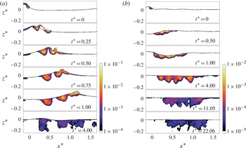
Figure 11. Snapshots of the normalized spanwise-averaged TKE,
 $\overline{k}$
, for (a) P1 (
$\overline{k}$
, for (a) P1 (
 $S=0.54$
) and (b) P3 (
$S=0.54$
) and (b) P3 (
 $S=0.352$
). The reference value is
$S=0.352$
). The reference value is
 $C_{c}^{2}$
.
$C_{c}^{2}$
.
4.3. Energy dissipation
Energy dissipation is one of the least understood components of the near-surface dynamics of the ocean. The breaking-induced dissipation rate is much greater than the other sources of dissipation especially during active breaking. In addition, breaking waves are highly intermittent in both time and space. Thus, the mixing and energy dissipation at the near-surface layer are highly intermittent and are dominated by the individual breaking events, with the background levels of turbulence and dissipation rate being considerably lower (Melville Reference Melville1994). Based on scaling arguments, Duncan (Reference Duncan1983) showed that the wave dissipation per unit length of breaking crest can be written in the form
 $$\begin{eqnarray}\check{{\it\epsilon}}_{total}=b{\it\rho}g^{-1}c_{b}^{5},\end{eqnarray}$$
where
 $g$
is the gravitational acceleration,
$g$
is the gravitational acceleration,
 $c_{b}$
is the phase speed of the breaking wave and
$c_{b}$
is the phase speed of the breaking wave and
 $b$
is a breaking parameter. Phillips (Reference Phillips1985) defined a distribution
$b$
is a breaking parameter. Phillips (Reference Phillips1985) defined a distribution
 ${\it\Lambda}(c_{b})$
so that
${\it\Lambda}(c_{b})$
so that
 ${\it\Lambda}(c_{b})\text{d}c_{b}$
represents the average total length of breaking fronts per unit surface area travelling with velocities in the range
${\it\Lambda}(c_{b})\text{d}c_{b}$
represents the average total length of breaking fronts per unit surface area travelling with velocities in the range
 $(c_{b},c_{b}+\text{d}c_{b})$
. He then formulated the average rate of energy loss for breaking waves with speeds in the range
$(c_{b},c_{b}+\text{d}c_{b})$
. He then formulated the average rate of energy loss for breaking waves with speeds in the range
 $(c_{b},c_{b}+\text{d}c_{b})$
per unit surface area as
$(c_{b},c_{b}+\text{d}c_{b})$
per unit surface area as
 $$\begin{eqnarray}\check{{\it\epsilon}}_{total}(c_{b})\text{d}c_{b}=b{\it\rho}g^{-1}c_{b}^{5}{\it\Lambda}(c_{b})\text{d}c_{b}.\end{eqnarray}$$
This concept is interesting especially for large-scale models with relatively large time scales, e.g. wind–wave models in which a whole breaking event is SGS and needs to be parameterized based on the spectral characteristics. However, as summarized by Drazen et al. (Reference Drazen, Melville and Lenain2008), the available literature shows a large scatter for
 $b$
. In addition, so far only a few published
$b$
. In addition, so far only a few published
 ${\it\Lambda}(c_{b})$
distributions exist, and it may need to be calibrated based on the specific area of interest.
${\it\Lambda}(c_{b})$
distributions exist, and it may need to be calibrated based on the specific area of interest.
In this section, we first examine the bubble- and shear-induced dissipation and their contribution to the total dissipation under a breaking event – the former is commonly ignored in 3D LES simulations of breaking waves. Then, we discuss the time-dependent behaviour of the breaking parameter,
 $b$
. In addition, a scaling law for the time-averaged dissipation rate per unit length of breaking crest is obtained.
$b$
. In addition, a scaling law for the time-averaged dissipation rate per unit length of breaking crest is obtained.
4.3.1. Shear- and bubble-induced dissipation
The dissipation rate of the resolved kinetic energy per unit mass is
 $$\begin{eqnarray}{\it\varepsilon}_{total}={\it\varepsilon}_{r}+{\it\varepsilon}_{sgs},\end{eqnarray}$$
where
 ${\it\varepsilon}_{r}=2{\it\nu}\mathscr{S}_{ij}\mathscr{S}_{ij}={\it\nu}|\mathscr{S}|^{2}$
is the viscous dissipation rate directly from the resolved velocity field, and
${\it\varepsilon}_{r}=2{\it\nu}\mathscr{S}_{ij}\mathscr{S}_{ij}={\it\nu}|\mathscr{S}|^{2}$
is the viscous dissipation rate directly from the resolved velocity field, and
 ${\it\varepsilon}_{sgs}$
represents the rate of transfer of energy from the resolved motions to the SGS motions. In the present study,
${\it\varepsilon}_{sgs}$
represents the rate of transfer of energy from the resolved motions to the SGS motions. In the present study,
 ${\it\varepsilon}_{sgs}=-{\it\tau}_{ij}^{d}\mathscr{S}_{ij}={\it\varepsilon}_{SI}+{\it\varepsilon}_{BI}$
consists of two different dissipation mechanisms. Here,
${\it\varepsilon}_{sgs}=-{\it\tau}_{ij}^{d}\mathscr{S}_{ij}={\it\varepsilon}_{SI}+{\it\varepsilon}_{BI}$
consists of two different dissipation mechanisms. Here,
 ${\it\varepsilon}_{SI}={\it\nu}_{SI}|\mathscr{S}|^{2}$
is a conventional shear-induced dissipation rate similar to a single-phase turbulence. The additional term,
${\it\varepsilon}_{SI}={\it\nu}_{SI}|\mathscr{S}|^{2}$
is a conventional shear-induced dissipation rate similar to a single-phase turbulence. The additional term,
 ${\it\varepsilon}_{BI}={\it\nu}_{BI}|\mathscr{S}|^{2}$
, accounts for turbulent SGS motions generated by the dispersed bubbles and enhances the dissipation rate. At high Reynolds number, with the filter width much larger than the Kolmogorov length scale (typical in LES),
${\it\varepsilon}_{BI}={\it\nu}_{BI}|\mathscr{S}|^{2}$
, accounts for turbulent SGS motions generated by the dispersed bubbles and enhances the dissipation rate. At high Reynolds number, with the filter width much larger than the Kolmogorov length scale (typical in LES),
 ${\it\varepsilon}_{r}$
is usually negligibly small, and if the model resolves most of the TKE, we can approximate the total dissipation rate,
${\it\varepsilon}_{r}$
is usually negligibly small, and if the model resolves most of the TKE, we can approximate the total dissipation rate,
 ${\it\varepsilon}$
, by
${\it\varepsilon}$
, by
 $\overline{{\it\varepsilon}_{sgs}}$
. This is equivalent to assuming that there is a close balance between production and dissipation in the averaged kinetic energy of SGS motions (Pope Reference Pope2000).
$\overline{{\it\varepsilon}_{sgs}}$
. This is equivalent to assuming that there is a close balance between production and dissipation in the averaged kinetic energy of SGS motions (Pope Reference Pope2000).
Figure 12 shows snapshots of the spatial distribution of
 $\overline{{\it\varepsilon}_{sgs}}$
for P1 with and without the inclusion of a dispersed bubble phase. The regions with a high dissipation rate are collocated with the high vorticity and TKE regions. Here,
$\overline{{\it\varepsilon}_{sgs}}$
for P1 with and without the inclusion of a dispersed bubble phase. The regions with a high dissipation rate are collocated with the high vorticity and TKE regions. Here,
 $\overline{{\it\varepsilon}_{sgs}}$
is large,
$\overline{{\it\varepsilon}_{sgs}}$
is large,
 $O(1\ \text{m}^{2}\ \text{s}^{-3})$
, at the jet/splash impact and the bore-front regions. These regions have a relatively high void fraction, and comparing the results of the simulation with and without a bubble phase clearly shows enhancement of the dissipation rate in these bubbly regions. The local values of the dissipation rate decrease quickly. At the end of active breaking, they become at least two orders of magnitude smaller. The corresponding Hinze scale of the bubble radius then can be estimated as
$O(1\ \text{m}^{2}\ \text{s}^{-3})$
, at the jet/splash impact and the bore-front regions. These regions have a relatively high void fraction, and comparing the results of the simulation with and without a bubble phase clearly shows enhancement of the dissipation rate in these bubbly regions. The local values of the dissipation rate decrease quickly. At the end of active breaking, they become at least two orders of magnitude smaller. The corresponding Hinze scale of the bubble radius then can be estimated as
 $a_{H}\cong c({\it\gamma}/{\it\rho})^{3/5}{\it\varepsilon}^{-2/5}\approx 1\ \text{mm}$
, where
$a_{H}\cong c({\it\gamma}/{\it\rho})^{3/5}{\it\varepsilon}^{-2/5}\approx 1\ \text{mm}$
, where
 $c=0.36{-}0.5$
and
$c=0.36{-}0.5$
and
 ${\it\gamma}/{\it\rho}=7.3\times 10^{-5}$
(see Garrett, Li & Farmer Reference Garrett, Li and Farmer2000). This is consistent with our choice of
${\it\gamma}/{\it\rho}=7.3\times 10^{-5}$
(see Garrett, Li & Farmer Reference Garrett, Li and Farmer2000). This is consistent with our choice of
 $a_{H}=1\ \text{mm}$
for the bubble size distribution.
$a_{H}=1\ \text{mm}$
for the bubble size distribution.
Figure 13 shows the integrated viscous as well as shear- and bubble-induced SGS dissipation rates in the breaking region for P1, SP1 and S1. The bubble-induced dissipation is noticeable during the jet/splash cycles at which a large volume of bubbles is entrained. At the end of active breaking, when the bore-like region is formed, bubble-induced dissipation becomes large and comparable with shear-induced dissipation, again. At later times, at which the surface waves have passed the breaking region (
 $t^{\ast }>4$
), the total dissipation rate of the background turbulence seems to decay like
$t^{\ast }>4$
), the total dissipation rate of the background turbulence seems to decay like
 $(t^{\ast })^{n}$
, where
$(t^{\ast })^{n}$
, where
 $n$
is initially approximately
$n$
is initially approximately
 $-2.5$
, but becomes close to the theoretical value for isotropic turbulence,
$-2.5$
, but becomes close to the theoretical value for isotropic turbulence,
 $n=-17/4$
(Gemmrich & Farmer Reference Gemmrich and Farmer2004), for
$n=-17/4$
(Gemmrich & Farmer Reference Gemmrich and Farmer2004), for
 $t^{\ast }>12$
. As we would expect, the viscous dissipation rate is small compared with the SGS dissipation rate.
$t^{\ast }>12$
. As we would expect, the viscous dissipation rate is small compared with the SGS dissipation rate.

Figure 12. Snapshots of the spanwise-averaged SGS dissipation rate,
 $\overline{{\it\varepsilon}_{sgs}}\ (\text{m}^{2}\ \text{s}^{-3})$
, for P1, from the simulation (a) with and (b) without the inclusion of the dispersed bubbles.
$\overline{{\it\varepsilon}_{sgs}}\ (\text{m}^{2}\ \text{s}^{-3})$
, for P1, from the simulation (a) with and (b) without the inclusion of the dispersed bubbles.

Figure 13. Dissipation rate per unit length of crest due to the different mechanisms for (a) P1, (b) SP1 and (c) S1: ——, shear-induced
 $\check{\overline{{\it\varepsilon}_{SI}}}/L_{c}^{2}$
; – – –, bubble-induced
$\check{\overline{{\it\varepsilon}_{SI}}}/L_{c}^{2}$
; – – –, bubble-induced
 $\check{\overline{{\it\varepsilon}_{BI}}}/L_{c}^{2}$
; — ⋅ —, viscous dissipation
$\check{\overline{{\it\varepsilon}_{BI}}}/L_{c}^{2}$
; — ⋅ —, viscous dissipation
 $\check{\overline{{\it\varepsilon}_{r}}}/L_{c}^{2}$
. The dashed lines indicate
$\check{\overline{{\it\varepsilon}_{r}}}/L_{c}^{2}$
. The dashed lines indicate
 $(t^{\ast })^{n}$
, where
$(t^{\ast })^{n}$
, where
 $n$
is the number on the lines.
$n$
is the number on the lines.
The total breaking-induced viscous,
 $\hat{{\it\epsilon}}_{r}$
, and SGS dissipation,
$\hat{{\it\epsilon}}_{r}$
, and SGS dissipation,
 $\hat{{\it\epsilon}}_{sgs}$
, per unit length of crest can be calculated using
$\hat{{\it\epsilon}}_{sgs}$
, per unit length of crest can be calculated using
 $$\begin{eqnarray}\displaystyle \hat{{\it\epsilon}}_{r}(t^{\ast }) & = & \displaystyle \int _{t_{0}^{\ast }}^{t^{\ast }}\int _{A}{\it\epsilon}_{r}\text{d}A\text{d}t^{\ast }=\int _{t_{0}^{\ast }}^{t^{\ast }}\int _{A}\overline{{\it\alpha}{\it\rho}{\it\varepsilon}_{r}}\text{d}A\text{d}t^{\ast },\end{eqnarray}$$
 $$\begin{eqnarray}\displaystyle \hat{{\it\epsilon}}_{sgs}(t^{\ast }) & = & \displaystyle \int _{t_{0}^{\ast }}^{t^{\ast }}\int _{A}{\it\epsilon}_{sgs}\text{d}A\text{d}t^{\ast }=\int _{t_{0}^{\ast }}^{t^{\ast }}\int _{A}\overline{{\it\alpha}{\it\rho}{\it\varepsilon}_{sgs}}\text{d}A\text{d}t^{\ast },\end{eqnarray}$$
 $t_{0}^{\ast }=-0.25$
and
$t_{0}^{\ast }=-0.25$
and
 ${\it\alpha}{\it\rho}$
is the density of the liquid phase at each grid point. Figure 14 shows the results for P1, SP1 and S1. In all the breaker types, most of the energy is dissipated (more that 80 % of the total dissipation) during the first period after breaking, with the bubble-induced dissipation larger than the shear-induced dissipation. Table 6 summarizes the different dissipation contributions predicted by the model and the estimation from LM. Comparing with the experimental estimations, we can conclude that the simulations without the inclusion of the dispersed bubbles underpredict the total dissipation by approximately 35 % in both plunging and spilling breaking. In addition, bubble-induced dissipation accounts for more than 50 % of the total breaking-induced dissipation regardless of the breaker’s type and intensity. We should note that the cavity breakup process is not resolved in our simulations, and may be responsible for an additional dissipation during the initial stage of active breaking.
${\it\alpha}{\it\rho}$
is the density of the liquid phase at each grid point. Figure 14 shows the results for P1, SP1 and S1. In all the breaker types, most of the energy is dissipated (more that 80 % of the total dissipation) during the first period after breaking, with the bubble-induced dissipation larger than the shear-induced dissipation. Table 6 summarizes the different dissipation contributions predicted by the model and the estimation from LM. Comparing with the experimental estimations, we can conclude that the simulations without the inclusion of the dispersed bubbles underpredict the total dissipation by approximately 35 % in both plunging and spilling breaking. In addition, bubble-induced dissipation accounts for more than 50 % of the total breaking-induced dissipation regardless of the breaker’s type and intensity. We should note that the cavity breakup process is not resolved in our simulations, and may be responsible for an additional dissipation during the initial stage of active breaking.

Figure 14. Total breaking-induced dissipation per unit length of crest (
 $\text{J}\ \text{m}^{-1}$
) for (a) P1, (b) SP1 and (c) S1: ——,
$\text{J}\ \text{m}^{-1}$
) for (a) P1, (b) SP1 and (c) S1: ——,
 $\hat{{\it\epsilon}}_{total}=\hat{{\it\epsilon}}_{r}+\hat{{\it\epsilon}}_{sgs}$
; – – –,
$\hat{{\it\epsilon}}_{total}=\hat{{\it\epsilon}}_{r}+\hat{{\it\epsilon}}_{sgs}$
; – – –,
 $\hat{{\it\epsilon}}_{sgs}^{SI}$
; — ⋅ —,
$\hat{{\it\epsilon}}_{sgs}^{SI}$
; — ⋅ —,
 $\hat{{\it\epsilon}}_{sgs}^{BI}$
;
$\hat{{\it\epsilon}}_{sgs}^{BI}$
;
 $\cdots \cdots \,$
,
$\cdots \cdots \,$
,
 $\hat{{\it\epsilon}}_{r}$
;——,
$\hat{{\it\epsilon}}_{r}$
;——,
 $\hat{{\it\epsilon}}_{total}^{nb}$
(the total dissipation from the simulations without the inclusion of the dispersed bubbles).
$\hat{{\it\epsilon}}_{total}^{nb}$
(the total dissipation from the simulations without the inclusion of the dispersed bubbles).
Table 6. Total dissipation in the breaking region. LM approximated the total dissipation by estimating the total energy flux difference between upstream and downstream of the breaking region.

4.3.2. Time-dependent breaking parameter,
 $b$
$b$

Available estimates of the breaking parameter
 $b$
range from
$b$
range from
 $O(10^{-4})$
to
$O(10^{-4})$
to
 $O(10^{-2})$
, depending on the breaking type and intensity, the unsteady or quasi-steady character, and probably the method of defining the breaking parameter. In most of the previous experiments, the total breaking-induced dissipation per unit length of breaking crest,
$O(10^{-2})$
, depending on the breaking type and intensity, the unsteady or quasi-steady character, and probably the method of defining the breaking parameter. In most of the previous experiments, the total breaking-induced dissipation per unit length of breaking crest,
 $\hat{{\it\epsilon}}_{total}$
, was approximated through surface elevation measurements at fixed locations upstream and downstream of the wave breaking and by implementation of a wave theory and a simple control volume analysis. The averaged dissipation rate,
$\hat{{\it\epsilon}}_{total}$
, was approximated through surface elevation measurements at fixed locations upstream and downstream of the wave breaking and by implementation of a wave theory and a simple control volume analysis. The averaged dissipation rate,
 $\overline{\overline{\check{{\it\epsilon}}}}_{total}$
, then, is defined as
$\overline{\overline{\check{{\it\epsilon}}}}_{total}$
, then, is defined as
 $\overline{\overline{\check{{\it\epsilon}}}}_{total}=\hat{{\it\epsilon}}_{total}/{\it\tau}_{b}$
, where
$\overline{\overline{\check{{\it\epsilon}}}}_{total}=\hat{{\it\epsilon}}_{total}/{\it\tau}_{b}$
, where
 ${\it\tau}_{b}$
is a time scale related to the active breaking period and is of the order of the breaking wave period,
${\it\tau}_{b}$
is a time scale related to the active breaking period and is of the order of the breaking wave period,
 $T$
;
$T$
;
 $\hat{(\ )}$
,
$\hat{(\ )}$
,
 $\check{(\ )}$
and
$\check{(\ )}$
and
 $\overline{\overline{(\ )}}$
represent time and space integration, space integration and time averaging, respectively. Finally, the time-averaged breaking parameter,
$\overline{\overline{(\ )}}$
represent time and space integration, space integration and time averaging, respectively. Finally, the time-averaged breaking parameter,
 $\overline{\overline{b}}$
, is defined as
$\overline{\overline{b}}$
, is defined as
 $$\begin{eqnarray}\overline{\overline{b}}=\frac{g\overline{\overline{\check{{\it\epsilon}}}}_{total}}{{\it\rho}c_{b}^{5}}.\end{eqnarray}$$
For example, Drazen et al. (Reference Drazen, Melville and Lenain2008) estimated
 $\hat{{\it\epsilon}}_{total}\approx -{\rm\Delta}F_{b}={\it\rho}gC_{g_{s}}\int _{t_{1}}^{t_{2}}({\it\eta}_{2}^{2}-{\it\eta}_{1}^{2})\text{d}t$
, where
$\hat{{\it\epsilon}}_{total}\approx -{\rm\Delta}F_{b}={\it\rho}gC_{g_{s}}\int _{t_{1}}^{t_{2}}({\it\eta}_{2}^{2}-{\it\eta}_{1}^{2})\text{d}t$
, where
 $C_{g_{s}}$
is the spectrally weighted group velocity. They chose
$C_{g_{s}}$
is the spectrally weighted group velocity. They chose
 ${\it\tau}_{b}$
equal to the acoustically active period as measured by a hydrophone.
${\it\tau}_{b}$
equal to the acoustically active period as measured by a hydrophone.

Figure 15. Different breaking parameters (a)
 $b$
, (b)
$b$
, (b)
 $b/(S-S_{0})$
, (c)
$b/(S-S_{0})$
, (c)
 ${\it\beta}$
and (d)
${\it\beta}$
and (d)
 $\overline{\overline{{\it\beta}}}$
for ——, P1; — ⋅ —, P2; – – –, SP1;
$\overline{\overline{{\it\beta}}}$
for ——, P1; — ⋅ —, P2; – – –, SP1;
 $\cdots \cdots \,$
, S1; ——, P3; - - -, S2.
$\cdots \cdots \,$
, S1; ——, P3; - - -, S2.
Here, we have time-dependent information on the breaking-induced dissipation rate. Thus, the time-dependent breaking parameter,
 $b$
, can be readily calculated as
$b$
, can be readily calculated as
 $$\begin{eqnarray}b=\frac{g\check{{\it\epsilon}}_{total}}{{\it\rho}c_{b}^{5}}.\end{eqnarray}$$
Figure 15(a) shows
 $b$
for the different breakers. For all breakers,
$b$
for the different breakers. For all breakers,
 $b$
decreases by approximately an order of magnitude at the end of active breaking compared with the initial stage of breaking. In addition, it is clear that
$b$
decreases by approximately an order of magnitude at the end of active breaking compared with the initial stage of breaking. In addition, it is clear that
 $b$
is strongly linked to the breaker intensity, e.g. the corresponding
$b$
is strongly linked to the breaker intensity, e.g. the corresponding
 $b$
for P1 is approximately two orders of magnitude greater than that for S2. Intuitively, the most important parameter that can be related to breaker intensity is wave steepness. This is also confirmed by experimental measurements for both constant-amplitude and constant-steepness wavepackets. P1, P2, SP1 and S1 are constant-steepness type packets with
$b$
for P1 is approximately two orders of magnitude greater than that for S2. Intuitively, the most important parameter that can be related to breaker intensity is wave steepness. This is also confirmed by experimental measurements for both constant-amplitude and constant-steepness wavepackets. P1, P2, SP1 and S1 are constant-steepness type packets with
 $S_{0}\approx 0.34$
, while P3 and S2 are constant-amplitude type packets with
$S_{0}\approx 0.34$
, while P3 and S2 are constant-amplitude type packets with
 $S_{0}\approx 0.25$
, where
$S_{0}\approx 0.25$
, where
 $S_{0}$
is the global steepness of incipient breaking. The results reveal that the rate of increase of the breaking-induced dissipation in the packets with
$S_{0}$
is the global steepness of incipient breaking. The results reveal that the rate of increase of the breaking-induced dissipation in the packets with
 $S_{0}=0.34$
is considerably greater than that in the packets with
$S_{0}=0.34$
is considerably greater than that in the packets with
 $S_{0}=0.25$
. Furthermore, linear dependence of the breaking-induced dissipation on
$S_{0}=0.25$
. Furthermore, linear dependence of the breaking-induced dissipation on
 $S-S_{0}$
is observed for the cases with the same
$S-S_{0}$
is observed for the cases with the same
 $S_{0}$
, as shown in figure 15(b). This trend can also be recognized in DM, figure 8, in which the normalized change in energy flux across the control volume increases more noticeably as
$S_{0}$
, as shown in figure 15(b). This trend can also be recognized in DM, figure 8, in which the normalized change in energy flux across the control volume increases more noticeably as
 $S_{0}$
increases slightly. Thus, we define
$S_{0}$
increases slightly. Thus, we define
 $$\begin{eqnarray}b={\it\beta}(S-S_{0})S_{0}^{{\it\alpha}},\end{eqnarray}$$
where
 ${\it\beta}$
is a time-dependent parameter and
${\it\beta}$
is a time-dependent parameter and
 ${\it\alpha}$
is a constant. Figure 15(c) shows the resultant
${\it\alpha}$
is a constant. Figure 15(c) shows the resultant
 ${\it\beta}$
with the choice of
${\it\beta}$
with the choice of
 ${\it\alpha}=4$
, for all the breakers. As we can see, the choice of
${\it\alpha}=4$
, for all the breakers. As we can see, the choice of
 ${\it\alpha}=4$
successfully confines the large variation of breaking parameter for the different breakers (figure 15
a), and the resultant
${\it\alpha}=4$
successfully confines the large variation of breaking parameter for the different breakers (figure 15
a), and the resultant
 ${\it\beta}$
has the same trend and values regardless of the breaker’s type and intensity.
${\it\beta}$
has the same trend and values regardless of the breaker’s type and intensity.
Usually, the use of a time-averaged value of the breaking parameter,
 $\overline{\overline{b}}$
, is more preferable in models with relatively large time scales, e.g. wind–wave models. We define
$\overline{\overline{b}}$
, is more preferable in models with relatively large time scales, e.g. wind–wave models. We define
 $$\begin{eqnarray}\overline{\overline{b}}(t^{\ast })=\frac{1}{t^{\ast }-t_{0}^{\ast }}\int _{t_{0}^{\ast }}^{t^{\ast }}b\text{d}t^{\ast }=\frac{1}{t^{\ast }-t_{0}^{\ast }}\int _{t_{0}^{\ast }}^{t^{\ast }}{\it\beta}(S-S_{0})S_{0}^{4}\text{d}t^{\ast }=\overline{\overline{{\it\beta}}}(t^{\ast })(S-S_{0})S_{0}^{4},\end{eqnarray}$$
where
 $t_{0}^{\ast }=-0.1$
. Figure 15(d) shows that
$t_{0}^{\ast }=-0.1$
. Figure 15(d) shows that
 $\overline{\overline{{\it\beta}}}$
is nearly invariant for the different plunging and spilling breakers, after
$\overline{\overline{{\it\beta}}}$
is nearly invariant for the different plunging and spilling breakers, after
 $t^{\ast }=0.3$
. The appropriate
$t^{\ast }=0.3$
. The appropriate
 $\check{{\it\epsilon}}_{total}$
in (4.8) should represent the averaged dissipation rate per unit length of breaking crest during the active bubble entrainment period, which is of the order of the breaking wave period. Thus, considering
$\check{{\it\epsilon}}_{total}$
in (4.8) should represent the averaged dissipation rate per unit length of breaking crest during the active bubble entrainment period, which is of the order of the breaking wave period. Thus, considering
 $\overline{\overline{{\it\beta}}}(t^{\ast }=0.5{-}1.0)\sim 3$
, the averaged breaking parameter becomes
$\overline{\overline{{\it\beta}}}(t^{\ast }=0.5{-}1.0)\sim 3$
, the averaged breaking parameter becomes
 $$\begin{eqnarray}\overline{\overline{b}}\cong 3(S-S_{0})S_{0}^{4}.\end{eqnarray}$$
Finally, the averaged breaking-induced dissipation rate per unit length of breaking crest in the active breaking period can be approximated as
 $$\begin{eqnarray}\overline{\overline{\check{{\it\epsilon}}}}_{total}\cong 3{\it\rho}g^{-1}c_{b}^{5}(S-S_{0})S_{0}^{4},\quad \text{for }S>S_{0},\end{eqnarray}$$
and for
 $S<S_{0}$
the packet is non-breaking and
$S<S_{0}$
the packet is non-breaking and
 $\overline{\overline{\check{{\it\epsilon}}}}_{total}=0$
.
$\overline{\overline{\check{{\it\epsilon}}}}_{total}=0$
.
4.4. Turbulence modulation by the dispersed bubbles
To examine turbulence modulation by dispersed bubbles, their effects on turbulence production by mean shear and SGS dissipation as well as the work done by the dispersed bubbles on turbulence motions (or turbulence production by dispersed bubbles) should be considered. In this section, the temporal variation of spatially integrated terms in the breaking region will be discussed. First, the comparisons of turbulence production, SGS dissipation and total TKE between the simulations with and without the inclusion of dispersed bubbles are presented. Then, the role of production by dispersed bubbles, which leads to different modulation of the total TKE in plunging and spilling breakers, will be discussed.
In LES, the transport equation for the resolved TKE can be obtained based on the resolved velocity field. Subgrid-scale dissipation contains both shear- and bubble-induced dissipation and typically is much larger than the viscous dissipation (figure 14). In the case of a two-phase flow with a dilute regime (
 ${\it\alpha}\approx 1$
), common practice is to use the conventional single-phase TKE transport equation with an additional term due to a correlation between the fluctuating concentration and the vertical turbulent velocity component,
${\it\alpha}\approx 1$
), common practice is to use the conventional single-phase TKE transport equation with an additional term due to a correlation between the fluctuating concentration and the vertical turbulent velocity component,
 $-{\it\rho}g\overline{{\it\alpha}^{\prime }w^{\prime }}$
, where hereafter
$-{\it\rho}g\overline{{\it\alpha}^{\prime }w^{\prime }}$
, where hereafter
 $\overline{(.)}$
indicates ensemble (spanwise)-averaged. As we have shown, highly turbulent and dissipative regions are collocated with high void fraction regions. Due to a large void fraction (
$\overline{(.)}$
indicates ensemble (spanwise)-averaged. As we have shown, highly turbulent and dissipative regions are collocated with high void fraction regions. Due to a large void fraction (
 ${>}\!10\,\%$
) during the active breaking period, the dilute assumption is not valid anymore, and concentration fluctuations cannot be ignored. The exact resolved TKE transport equation for a two-phase flow is derived in § A.2. The final equation is given by
${>}\!10\,\%$
) during the active breaking period, the dilute assumption is not valid anymore, and concentration fluctuations cannot be ignored. The exact resolved TKE transport equation for a two-phase flow is derived in § A.2. The final equation is given by
 $$\begin{eqnarray}\displaystyle \frac{\partial }{\partial t}({\it\rho}\bar{{\it\alpha}}\bar{k})+\frac{\partial }{\partial x_{j}}({\it\rho}\bar{{\it\alpha}}{\bar{u}}_{j}\bar{k}) & = & \displaystyle T^{k}+P^{k}+B^{k}+E^{k}-({\it\epsilon}_{r}^{k}+{\it\epsilon}_{sgs}^{k})+D^{k}\nonumber\\ \displaystyle & & \displaystyle +\,t_{ex}^{k}+T_{ex}^{k}+P_{ex}^{k}-({\it\epsilon}_{r,ex}^{k}+{\it\epsilon}_{sgs,ex}^{k})+D_{ex}^{k},\end{eqnarray}$$
where
 $k=u_{i}^{\prime }u_{i}^{\prime }/2$
is the resolved TKE. The other terms are given by (A 8) and (A 9) in § A.2. In the case of a single-phase flow,
$k=u_{i}^{\prime }u_{i}^{\prime }/2$
is the resolved TKE. The other terms are given by (A 8) and (A 9) in § A.2. In the case of a single-phase flow,
 $\bar{{\it\alpha}}=1$
and
$\bar{{\it\alpha}}=1$
and
 ${\it\alpha}^{\prime }=\partial {\bar{u}}_{j}/\partial x_{j}=\partial u_{j}^{\prime }/\partial x_{j}=0$
, by which the extra terms become zero and (4.18) reduces to the single-phase classical transport equation for the resolved TKE. The comparison between the estimated total turbulence production and SGS dissipation using (4.18) and the single-phase TKE transport equation, as well as the relative importance of the extra terms due to triple correlations in (4.18), are presented in appendix B.
${\it\alpha}^{\prime }=\partial {\bar{u}}_{j}/\partial x_{j}=\partial u_{j}^{\prime }/\partial x_{j}=0$
, by which the extra terms become zero and (4.18) reduces to the single-phase classical transport equation for the resolved TKE. The comparison between the estimated total turbulence production and SGS dissipation using (4.18) and the single-phase TKE transport equation, as well as the relative importance of the extra terms due to triple correlations in (4.18), are presented in appendix B.
Figure 16 shows the total production rate by mean shear,
 $\check{P}_{total}^{k}$
, and figure 17 shows the total SGS dissipation rate,
$\check{P}_{total}^{k}$
, and figure 17 shows the total SGS dissipation rate,
 $\check{{\it\epsilon}}_{total}^{k}$
, for the simulations both with and without the inclusion of the dispersed bubbles. The presence of dispersed bubbles reduces
$\check{{\it\epsilon}}_{total}^{k}$
, for the simulations both with and without the inclusion of the dispersed bubbles. The presence of dispersed bubbles reduces
 $\check{P}_{total}^{k}$
while enhancing
$\check{P}_{total}^{k}$
while enhancing
 $\check{{\it\epsilon}}_{total}^{k}$
in both plunging and spilling breakers. The total production rate by buoyancy
$\check{{\it\epsilon}}_{total}^{k}$
in both plunging and spilling breakers. The total production rate by buoyancy
 ${\check{E}}_{p}^{k}$
(not shown) is an order of magnitude smaller than that by mean shear and the dispersed bubbles.
${\check{E}}_{p}^{k}$
(not shown) is an order of magnitude smaller than that by mean shear and the dispersed bubbles.

Figure 16. The two-phase total production rate by mean shear,
 $\check{P}_{total}^{k}=\check{P}^{k}+\check{P}_{ex1}^{k}+\check{P}_{ex2}^{k}$
, from simulations —— with and – – – without the inclusion of the dispersed bubbles for (a) P1, (b) SP1 and (c) S1. The reference value is
$\check{P}_{total}^{k}=\check{P}^{k}+\check{P}_{ex1}^{k}+\check{P}_{ex2}^{k}$
, from simulations —— with and – – – without the inclusion of the dispersed bubbles for (a) P1, (b) SP1 and (c) S1. The reference value is
 ${\it\rho}L_{c}^{2}C_{c}^{2}T_{c}^{-1}$
.
${\it\rho}L_{c}^{2}C_{c}^{2}T_{c}^{-1}$
.

Figure 17. The two-phase total SGS dissipation rate by mean shear,
 $\check{{\it\epsilon}}_{total}^{k}=\check{{\it\epsilon}}^{k}+\check{{\it\epsilon}}_{ex1}^{k}+\check{{\it\epsilon}}_{ex2}^{k}$
, from simulations —— with and – – – without the inclusion of the dispersed bubbles for (a) P1, (b) SP1 and (c) S1. The reference value is
$\check{{\it\epsilon}}_{total}^{k}=\check{{\it\epsilon}}^{k}+\check{{\it\epsilon}}_{ex1}^{k}+\check{{\it\epsilon}}_{ex2}^{k}$
, from simulations —— with and – – – without the inclusion of the dispersed bubbles for (a) P1, (b) SP1 and (c) S1. The reference value is
 ${\it\rho}L_{c}^{2}C_{c}^{2}T_{c}^{-1}$
.
${\it\rho}L_{c}^{2}C_{c}^{2}T_{c}^{-1}$
.

Figure 18. Normalized total resolved TKE,
 ${\check{k}}$
, in the breaking region, from simulations —— with and – – – without the inclusion of the dispersed bubbles for (a) P1, (b) SP1 and (c) S1. The reference value is
${\check{k}}$
, in the breaking region, from simulations —— with and – – – without the inclusion of the dispersed bubbles for (a) P1, (b) SP1 and (c) S1. The reference value is
 $L_{c}^{2}C_{c}^{2}(S-S_{0})S_{0}^{4}$
.
$L_{c}^{2}C_{c}^{2}(S-S_{0})S_{0}^{4}$
.

Figure 19. Total spanwise-averaged interfacial forces exerted on the water column by the bubbles,
 $\check{F}_{i,type}^{m}$
, for P1 (
$\check{F}_{i,type}^{m}$
, for P1 (
 $S=0.54$
) in (a) the streamwise direction and (b) the vertical direction: ——, drag force; – – –, virtual mass force; — ⋅ —, lift force. The reference value is
$S=0.54$
) in (a) the streamwise direction and (b) the vertical direction: ——, drag force; – – –, virtual mass force; — ⋅ —, lift force. The reference value is
 ${\it\rho}L_{c}^{2}C_{c}T_{c}^{-1}$
.
${\it\rho}L_{c}^{2}C_{c}T_{c}^{-1}$
.
Figure 18 shows that the dispersed bubbles damp the total TKE by approximately 20–30 % in the plunging breakers and 50 % in the spilling breaker. An exception is for
 $t^{\ast }<0.5$
, where the TKE is damped slightly, or even enhanced in the large plunging case P1. This enhancement of the TKE in the large plunging case as well as the increase of TKE damping by decreasing breaking intensity can be explained through turbulence production by dispersed bubbles,
$t^{\ast }<0.5$
, where the TKE is damped slightly, or even enhanced in the large plunging case P1. This enhancement of the TKE in the large plunging case as well as the increase of TKE damping by decreasing breaking intensity can be explained through turbulence production by dispersed bubbles,
 $B^{k}=-\overline{f_{i}^{\prime }u_{i}^{\prime }}$
. Interfacial momentum transfer and turbulence production by dispersed bubbles through drag, virtual mass and lift forces are discussed in the following section. To summarize, positive
$B^{k}=-\overline{f_{i}^{\prime }u_{i}^{\prime }}$
. Interfacial momentum transfer and turbulence production by dispersed bubbles through drag, virtual mass and lift forces are discussed in the following section. To summarize, positive
 $B^{k}$
contributes to both the reduction of
$B^{k}$
contributes to both the reduction of
 $\check{P}_{total}^{k}$
and enhancement of
$\check{P}_{total}^{k}$
and enhancement of
 $\check{{\it\epsilon}}_{total}^{k}$
to some extent. In P1,
$\check{{\it\epsilon}}_{total}^{k}$
to some extent. In P1,
 $B^{k}$
is large (figure 21
d) during the entrainment stage, leading to the net enhancement of the total TKE for
$B^{k}$
is large (figure 21
d) during the entrainment stage, leading to the net enhancement of the total TKE for
 $t^{\ast }<0.5$
. However, in the spilling breaker, S1, this production by bubbles is relatively weak (figure 22
d) and the TKE is damped approximately half as much as in the simulation without the inclusion of dispersed bubbles. Finally, figure 18 reveals that the total TKE can also be scaled by
$t^{\ast }<0.5$
. However, in the spilling breaker, S1, this production by bubbles is relatively weak (figure 22
d) and the TKE is damped approximately half as much as in the simulation without the inclusion of dispersed bubbles. Finally, figure 18 reveals that the total TKE can also be scaled by
 $(S-S_{0})S_{0}^{4}$
, similarly to the averaged dissipation rate (4.17).
$(S-S_{0})S_{0}^{4}$
, similarly to the averaged dissipation rate (4.17).
4.5. Liquid–bubble momentum exchange and production by dispersed bubbles
Momentum exchange between the dispersed bubble phase and the liquid phase through drag, lift and virtual mass forces (2.19) is examined here. Using (2.17) and (2.18), the total spanwise-averaged forces,
 $\check{F}_{i,type}^{m}$
, exerted on the water column by the bubbles are calculated as
$\check{F}_{i,type}^{m}$
, exerted on the water column by the bubbles are calculated as
 $$\begin{eqnarray}\check{F}_{i,type}^{m}=\mathop{\sum }_{g=1}^{N_{G}}\int _{A}-\bar{f}_{i,type}^{g}\text{d}A,\end{eqnarray}$$
where
 $i$
refers to the
$i$
refers to the
 $x,y$
and
$x,y$
and
 $z$
directions, respectively; and
$z$
directions, respectively; and
 $type$
refers to the drag, virtual mass or lift forces. Figures 19 and 20 show the normalized
$type$
refers to the drag, virtual mass or lift forces. Figures 19 and 20 show the normalized
 $\check{F}_{i,type}^{m}$
for P1 and S1 in the streamwise and vertical directions. The main interphase exchange in the streamwise direction occurs during the bubble entrainment period, with
$\check{F}_{i,type}^{m}$
for P1 and S1 in the streamwise and vertical directions. The main interphase exchange in the streamwise direction occurs during the bubble entrainment period, with
 $|\check{F}_{x,drag}^{m}|\approx |\check{F}_{x,vmass}^{m}|$
. For P1 (figure 19
a), the interphase exchange during jet/splash impact,
$|\check{F}_{x,drag}^{m}|\approx |\check{F}_{x,vmass}^{m}|$
. For P1 (figure 19
a), the interphase exchange during jet/splash impact,
 $0<t^{\ast }<0.6$
, is an order of magnitude larger than that during the rest of the active breaking, when the previously entrained bubbles outgas continuously without any additional entrainment. At
$0<t^{\ast }<0.6$
, is an order of magnitude larger than that during the rest of the active breaking, when the previously entrained bubbles outgas continuously without any additional entrainment. At
 $t^{\ast }\sim 1$
, the bore front is formed and entrains some new bubbles with considerably smaller interphase momentum transfer. Such a strong temporal variation does not exist for the spilling case, S1 (figure 20
a). In the vertical direction, on the other hand, the drag force is the main interfacial feedback, with
$t^{\ast }\sim 1$
, the bore front is formed and entrains some new bubbles with considerably smaller interphase momentum transfer. Such a strong temporal variation does not exist for the spilling case, S1 (figure 20
a). In the vertical direction, on the other hand, the drag force is the main interfacial feedback, with
 $\check{F}_{z,drag}^{m}\gg \check{F}_{z,vmass}^{m}$
, and the spanwise-averaged drag force is noticeable during the whole active breaking period for both cases (figures 19
b and 20
b). Due to a relatively larger acceleration of the newly entrained bubbles compared with their surrounding liquid acceleration, the virtual mass force is mostly positive in the streamwise direction. The negative
$\check{F}_{z,drag}^{m}\gg \check{F}_{z,vmass}^{m}$
, and the spanwise-averaged drag force is noticeable during the whole active breaking period for both cases (figures 19
b and 20
b). Due to a relatively larger acceleration of the newly entrained bubbles compared with their surrounding liquid acceleration, the virtual mass force is mostly positive in the streamwise direction. The negative
 $\check{F}_{x,drag}^{m}$
is due to the negative relative velocity of the entrained bubbles in the streamwise direction compared with the liquid velocity. In the vertical direction, however, the relative velocity is mostly positive and is approximately equal to the rising velocity of the dispersed bubbles, leading to positive
$\check{F}_{x,drag}^{m}$
is due to the negative relative velocity of the entrained bubbles in the streamwise direction compared with the liquid velocity. In the vertical direction, however, the relative velocity is mostly positive and is approximately equal to the rising velocity of the dispersed bubbles, leading to positive
 $\check{F}_{z,drag}^{m}$
during the entire active breaking. Although the local values of the lift force are comparable with the other two forces, the spanwise-averaged lift force is negligibly small compared with the spanwise-averaged drag and virtual mass forces in both cases. The spanwise-averaged forces in the spanwise direction (not shown) are an order of magnitude smaller than those in the other two directions. The actual distribution of the forces is highly 3D; thus, the abovementioned arguments and the results presented in this section should be considered in an averaged sense.
$\check{F}_{z,drag}^{m}$
during the entire active breaking. Although the local values of the lift force are comparable with the other two forces, the spanwise-averaged lift force is negligibly small compared with the spanwise-averaged drag and virtual mass forces in both cases. The spanwise-averaged forces in the spanwise direction (not shown) are an order of magnitude smaller than those in the other two directions. The actual distribution of the forces is highly 3D; thus, the abovementioned arguments and the results presented in this section should be considered in an averaged sense.

Figure 20. Total spanwise-averaged interfacial forces exerted on the water column by the bubbles for S1 (
 $S=0.36$
). The definitions are the same as in figure 19.
$S=0.36$
). The definitions are the same as in figure 19.

Figure 21. The rate of work done on (a) the organized and (b) the turbulent motion by ——, the drag force; – – –, the virtual mass force; and — ⋅ —, the lift force for P1. The total rate of work done on (c) the organized,
 $\check{B}^{m}$
, and (d) the turbulent,
$\check{B}^{m}$
, and (d) the turbulent,
 $\check{B}^{k}$
, motion. The reference value is
$\check{B}^{k}$
, motion. The reference value is
 ${\it\rho}L_{c}^{2}C_{c}^{2}T_{c}^{-1}$
.
${\it\rho}L_{c}^{2}C_{c}^{2}T_{c}^{-1}$
.
The rates of total work done (or the rates of production) by the drag, virtual mass and lift forces on the organized flow,
 $\check{B}_{type}^{m}$
, and the turbulent motions,
$\check{B}_{type}^{m}$
, and the turbulent motions,
 $\check{B}_{type}^{k}$
, are given by
$\check{B}_{type}^{k}$
, are given by
 $$\begin{eqnarray}\check{B}_{type}^{m}=\mathop{\sum }_{i}\mathop{\sum }_{g=1}^{N_{G}}\int _{A}-\bar{f}_{i,type}^{g}{\bar{u}}_{i}\text{d}A,\quad \check{B}_{type}^{k}=\mathop{\sum }_{i}\mathop{\sum }_{g=1}^{N_{G}}\int _{A}-\overline{f_{i,type}^{\prime g}u_{i}^{\prime }}\text{d}A.\end{eqnarray}$$
Figures 21(a,b) and 22(a,b) show normalized
 $\check{B}_{type}^{m}$
and
$\check{B}_{type}^{m}$
and
 $\check{B}_{type}^{k}$
for P1 and S1 respectively. During the entrainment stage, the rates of total work done on the turbulent and organized motions by the virtual mass force,
$\check{B}_{type}^{k}$
for P1 and S1 respectively. During the entrainment stage, the rates of total work done on the turbulent and organized motions by the virtual mass force,
 $\check{B}_{vmass}^{m}$
and
$\check{B}_{vmass}^{m}$
and
 $\check{B}_{vmass}^{k}$
, are positive, while the corresponding rates of total work done by the drag and lift forces are mostly negative in both cases. The rates of total work done on the turbulent and organized motions by the lift force are negligibly small compared with those by the drag and virtual mass forces in both cases.
$\check{B}_{vmass}^{k}$
, are positive, while the corresponding rates of total work done by the drag and lift forces are mostly negative in both cases. The rates of total work done on the turbulent and organized motions by the lift force are negligibly small compared with those by the drag and virtual mass forces in both cases.

Figure 22. The rates of work done on the organized and turbulent motions by the dispersed bubbles for S1. The definitions are the same as in figure 21.
In the transport equations for the TKE and organized flow, the summations of all work done by the interfacial forces on organized,
 $\check{B}^{m}$
, and turbulent motions,
$\check{B}^{m}$
, and turbulent motions,
 $\check{B}^{k}$
, (see appendix A) are given by
$\check{B}^{k}$
, (see appendix A) are given by
 $$\begin{eqnarray}\check{B}^{m}=B_{drag}^{m}+B_{vmass}^{m}+B_{lift}^{m},\quad \check{B}^{k}=B_{drag}^{k}+B_{vmass}^{k}+B_{lift}^{k}.\end{eqnarray}$$
Figures 21(c,d) and 22(c,d) show the temporal variation of
 $\check{B}^{m}$
and
$\check{B}^{m}$
and
 $\check{B}^{k}$
for P1 and S1. During the jet/splash impact in P1,
$\check{B}^{k}$
for P1 and S1. During the jet/splash impact in P1,
 $\check{B}^{m}$
and
$\check{B}^{m}$
and
 $\check{B}^{k}$
are much greater than they are during the rest of the active breaking, with
$\check{B}^{k}$
are much greater than they are during the rest of the active breaking, with
 $\check{B}^{m}<\check{B}^{k}$
due to interaction between the 3D-distributed momentum exchange between two phases and the confused 3D velocity field. In the spilling case S1 and for
$\check{B}^{m}<\check{B}^{k}$
due to interaction between the 3D-distributed momentum exchange between two phases and the confused 3D velocity field. In the spilling case S1 and for
 $t^{\ast }>1$
in P1 at which the bore front is formed, on the other hand, there are nearly uniform production rates, with
$t^{\ast }>1$
in P1 at which the bore front is formed, on the other hand, there are nearly uniform production rates, with
 $\check{B}^{m}>\check{B}^{k}$
. As previously explained, the large positive
$\check{B}^{m}>\check{B}^{k}$
. As previously explained, the large positive
 $\check{B}^{k}$
during the jet/splash impact, which is comparable with the turbulence production by mean shear (figure 16
a), contributes to the enhancement of
$\check{B}^{k}$
during the jet/splash impact, which is comparable with the turbulence production by mean shear (figure 16
a), contributes to the enhancement of
 $\check{{\it\epsilon}}_{total}^{k}$
and the reduction of
$\check{{\it\epsilon}}_{total}^{k}$
and the reduction of
 $\check{P}_{total}^{k}$
by dispersed bubbles. In the spilling case,
$\check{P}_{total}^{k}$
by dispersed bubbles. In the spilling case,
 $\check{B}^{k}$
is much smaller compared with the corresponding
$\check{B}^{k}$
is much smaller compared with the corresponding
 $\check{P}_{total}^{k}$
. Although the structure of the bubble plume and the corresponding momentum exchange, as well as the velocity field behind the bore-front region, are 3D (see figure 3), the resultant
$\check{P}_{total}^{k}$
. Although the structure of the bubble plume and the corresponding momentum exchange, as well as the velocity field behind the bore-front region, are 3D (see figure 3), the resultant
 $\check{B}^{k}$
is relatively small due to very small bubble void fractions in these regions. In the bore-front region, instead, the momentum exchange and velocity field are nearly uniform in the spanwise direction, which leads to more pronounced positive work done on the organized motion in S1 (figures 22
c,d).
$\check{B}^{k}$
is relatively small due to very small bubble void fractions in these regions. In the bore-front region, instead, the momentum exchange and velocity field are nearly uniform in the spanwise direction, which leads to more pronounced positive work done on the organized motion in S1 (figures 22
c,d).
5. Conclusions
A continuum polydisperse two-fluid model was used to study turbulent bubbly flows under laboratory-scale isolated deep water breaking waves imposed by the focused wave method. Bubbles were entrained at the free surface using the bubble entrainment model. The free surface was captured by the second-order VOF interface tracking scheme. Turbulence was simulated using an LES approach with a dynamic Smagorinsky subgrid formulation. The SGS bubble-induced turbulence and dissipation as well as the momentum transfer between the two phases were considered. The main conclusions can be summarized in the following categories.
-
(a) Bubble entrainment and transport: it was shown that the entrainment model can predict the correct volume of entrained bubbles during the jet/splash impacts and in the bore-like region for the plunging and plunging/spilling breakers. The initial cavity entrapment is not a turbulence-related entrainment mechanism and can be captured by the VOF model. Since air entrainment in the spilling cases is mainly due to surface irregularity and bubble entrainment in the bore-like region is the dominant entrainment mechanism, we may expect that the entrainment model will also predict the correct volume of entrained air for spilling breakers during the entire entrainment period. By comparing snapshots of the void fraction distributions, void fraction time series as well as integral properties of the bubble plumes with the corresponding experiments, we can conclude that the model captures the spatial and temporal evolution of entrained bubbles fairly accurately.
-
(b) Dissipation: in all the breaker types, most of the energy (more than 80 % of the total dissipation) was dissipated during the first period after breaking. It was shown that the bubble-induced dissipation accounted for more than 50 % of the total dissipation. The bubble-induced dissipation rate was noticeable during the jet/splash cycles in which a large volume of bubbles was entrained. At the end of the active breaking, when the bore-like region was formed, the bubble-induced dissipation rate became large and comparable with the shear-induced dissipation rate, again.
In addition, the averaged dissipation rate per unit length of breaking crest is usually written as
$b{\it\rho}g^{-1}c_{b}^{5}$
. The breaking parameter,
$b$
, has been poorly constrained by experiments and field measurements. The time-dependent evolution of
$b$
was examined for both constant-steepness and constant-amplitude wavepackets. A scaling law for the averaged breaking parameter was obtained as
$\overline{\overline{b}}\cong 3(S-S_{0})S_{0}^{4}$
, where
$S={\it\Sigma}a_{i}k_{i}$
is the global steepness of the packet and
$S_{0}$
is the global steepness of incipient breaking. -
(c) Turbulence modulation by dispersed bubbles: all of the 3D simulations were repeated without the inclusion of dispersed bubbles, and it was shown that the integrated TKE in the breaking region was damped by the dispersed bubbles by approximately 20 % for the large plunging breaker to 50 % for the spilling breaker. In the plunging breakers, the TKE was damped only slightly or even enhanced during the initial stage of the active breaking. This was explained through the noticeable turbulence production by the dispersed bubbles in the larger plunging breakers during the initial stage of the active breaking.
-
(d) Liquid–bubble momentum exchange: in both spilling and plunging breakers, the drag force was the main interfacial feedback in the vertical direction. In the streamwise direction, the momentum exchange was noticeable during the initial stage of the active breaking with the spanwise-averaged total drag and virtual mass forces of the same order but in the opposite direction. Although the local values of the lift force were comparable with the other two forces, the spanwise-averaged lift force was negligibly small compared with the spanwise-averaged drag and virtual mass forces in both spilling and plunging breakers. The rates of total work done by the drag and lift forces were mostly negative while the rate of work done by the virtual mass force was positive in both the spilling and plunging breakers. In the plunging breakers, the rates of total work done on the organized flow,
$\check{B}^{m}$
, and turbulent motions,
$\check{B}^{k}$
, during the jet/splash impact were much greater than they were during the rest of the active breaking, with
$\check{B}^{m}<\check{B}^{k}$
. In the spilling cases, on the other hand, there were nearly uniform production rates, with
$\check{B}^{m}>\check{B}^{k}$
. -
(e) The two-phase versus single-phase TKE transport equation: due to a large void fraction (
${>}10\,\%$
) during the active breaking, the dilute assumption is not valid anymore, and concentration fluctuations cannot be ignored. It was found that in the high void fraction regions, the SGS dissipation rate was overpredicted by approximately 30 % to 50 % by the single-phase TKE transport equation. The total production rate by mean shear was also overpredicted by the single-phase formulation but the overprediction was smaller than 10 %.


Acknowledgements
This work was supported by The Office of Naval Research, Littoral Geosciences and Optics Program (grants N00014-10-1-0088 and N00014-13-1-0124). This research was supported in part through the use of computational resources provided by Information Technologies at the University of Delaware.
Appendix A. Exact transport equations for turbulent bubbly flow
The Reynolds decomposition of the resolved field
 $\tilde{{\it\phi}}=\langle \tilde{{\it\phi}}\rangle +\tilde{{\it\phi}}^{\prime }$
is used to separate organized and turbulent motions, where
$\tilde{{\it\phi}}=\langle \tilde{{\it\phi}}\rangle +\tilde{{\it\phi}}^{\prime }$
is used to separate organized and turbulent motions, where
 $\langle \ \rangle$
could be ensemble or phase averaging and here is approximated by spanwise averaging given by (2.35). All the variables are the liquid phase resolved quantities and for simplicity we drop
$\langle \ \rangle$
could be ensemble or phase averaging and here is approximated by spanwise averaging given by (2.35). All the variables are the liquid phase resolved quantities and for simplicity we drop
 $\tilde{(\ )}$
and
$\tilde{(\ )}$
and
 $(\ )^{l}$
.
$(\ )^{l}$
.
A.1. Transport equation for the averaged resolved kinetic energy
The resolved kinetic energy per unit mass (
 $e_{k}=u_{i}u_{i}/2$
) equation can be obtained by multiplying the liquid phase momentum equation, (2.14), by
$e_{k}=u_{i}u_{i}/2$
) equation can be obtained by multiplying the liquid phase momentum equation, (2.14), by
 $u_{i}$
,
$u_{i}$
,
 $$\begin{eqnarray}u_{i}\times \left[\underbrace{\frac{\partial ({\it\rho}{\it\alpha}u_{i})}{\partial t}}_{a}+\underbrace{\frac{\partial ({\it\rho}{\it\alpha}u_{i}u_{j})}{\partial x_{j}}}_{b}=\underbrace{-\frac{\partial ({\it\alpha}P)}{\partial x_{j}}{\it\delta}_{ij}}_{c}+\underbrace{{\it\rho}{\it\alpha}g_{i}}_{d}+\underbrace{\frac{\partial }{\partial x_{j}}\left[{\it\rho}{\it\alpha}(2{\it\nu}\mathscr{S}_{ij}-{\it\tau}_{ij}^{d})\right]}_{e}\underbrace{-f_{i}}_{f}\right],\end{eqnarray}$$
where
 $P=p+(2/3){\it\rho}k_{sgs}$
is the modified pressure,
$P=p+(2/3){\it\rho}k_{sgs}$
is the modified pressure,
 $-{\it\tau}_{ij}^{d}=2{\it\nu}_{sgs}\mathscr{S}_{ij}$
is the deviatoric part of the SGS stress tensor and
$-{\it\tau}_{ij}^{d}=2{\it\nu}_{sgs}\mathscr{S}_{ij}$
is the deviatoric part of the SGS stress tensor and
 $f_{i}$
is the hydrodynamic force exerted on the dispersed bubbles. By using the chain rule and
$f_{i}$
is the hydrodynamic force exerted on the dispersed bubbles. By using the chain rule and
 $A(\partial AB/\partial x)=\partial CB/\partial x+C(\partial B/\partial x)$
, where
$A(\partial AB/\partial x)=\partial CB/\partial x+C(\partial B/\partial x)$
, where
 $C=A^{2}/2$
, we obtain
$C=A^{2}/2$
, we obtain
 $$\begin{eqnarray}\displaystyle \left.\begin{array}{@{}l@{}}\displaystyle u_{i}\times a:\frac{\partial {\it\rho}{\it\alpha}e_{k}}{\partial t}+e_{k}\frac{\partial {\it\rho}{\it\alpha}}{\partial t},\\ \displaystyle u_{i}\times b:\frac{\partial {\it\rho}{\it\alpha}u_{j}e_{k}}{\partial x_{j}}+e_{k}\frac{\partial {\it\rho}{\it\alpha}u_{j}}{\partial x_{j}},\\ \displaystyle u_{i}\times c:-\frac{\partial {\it\alpha}Pu_{j}}{\partial x_{j}}+{\it\alpha}P\frac{\partial u_{j}}{\partial x_{j}},\\ u_{i}\times d:{\it\rho}{\it\alpha}g_{i}u_{i},\\ \displaystyle u_{i}\times e:\frac{\partial }{\partial x_{j}}\left[{\it\rho}{\it\alpha}(2{\it\nu}\mathscr{S}_{ij}-{\it\tau}_{ij}^{d})u_{i}\right]-{\it\rho}{\it\alpha}(2{\it\nu}\mathscr{S}_{ij}\mathscr{S}_{ij}-{\it\tau}_{ij}^{d}\mathscr{S}_{ij}),\\ u_{i}\times f:-f_{i}u_{i}.\end{array}\right\} & & \displaystyle\end{eqnarray}$$
Using the continuity equation (2.13) the summation of
 $e_{k}(\partial /\partial )$
terms is equal to zero, and the transport equation of averaged resolved kinetic energy is obtained by averaging the remaining terms of (A 2) as
$e_{k}(\partial /\partial )$
terms is equal to zero, and the transport equation of averaged resolved kinetic energy is obtained by averaging the remaining terms of (A 2) as
 $$\begin{eqnarray}\frac{\partial }{\partial t}({\it\rho}\overline{{\it\alpha}e_{k}})+\frac{\partial }{\partial x_{j}}({\it\rho}\overline{{\it\alpha}u_{j}e_{k}})=T-({\it\epsilon}_{r}+{\it\epsilon}_{sgs})+D+B+E,\end{eqnarray}$$
where
 $$\begin{eqnarray}\displaystyle \left.\begin{array}{@{}rcl@{}}T\, & =\, & \displaystyle -\frac{\partial }{\partial x_{j}}\left[\overline{{\it\alpha}Pu_{j}}-{\it\rho}\overline{{\it\alpha}(2{\it\nu}\mathscr{S}_{ij}-{\it\tau}_{ij}^{d})u_{i}}\right]\quad \\ \, & \, & \text{(rate of work done by pressure and viscous stresses),}\\ {\it\epsilon}_{r}\, & =\, & 2{\it\rho}\overline{{\it\alpha}{\it\nu}\mathscr{S}_{ij}\mathscr{S}_{ij}}\quad \text{(viscous dissipation rate),}\\ {\it\epsilon}_{sgs}\, & =\, & -{\it\rho}\overline{{\it\alpha}{\it\tau}_{ij}^{d}\mathscr{S}_{ij}}\quad \text{(SGS dissipation rate),}\\ D\, & =\, & \overline{{\it\alpha}P\frac{\displaystyle \partial u_{j}}{\displaystyle \partial x_{j}}}\quad \text{(pressure dilatation rate),}\\ B\, & =\, & -\overline{f_{i}u_{i}}\quad \text{(rate of work done by dispersed bubbles),}\\ E\, & =\, & \displaystyle {\it\rho}\overline{{\it\alpha}g_{i}u_{i}}=\frac{\text{D}}{\text{D}t}(-{\it\rho}\overline{{\it\alpha}e_{p}})\quad \\ \, & \, & \text{(rate of the total change of the potential energy),}\end{array}\right\} & & \displaystyle\end{eqnarray}$$
where
 $e_{p}=gz$
is the potential energy per unit mass and
$e_{p}=gz$
is the potential energy per unit mass and
 $g=|g_{3}|$
.
$g=|g_{3}|$
.
A.2. Transport equation for the resolved TKE
The transport equation for the averaged resolved TKE per unit mass,
 $\bar{k}=\overline{u_{i}^{\prime }u_{i}^{\prime }}/2$
, is obtained by multiplying the liquid phase momentum equation by
$\bar{k}=\overline{u_{i}^{\prime }u_{i}^{\prime }}/2$
, is obtained by multiplying the liquid phase momentum equation by
 $u_{i}^{\prime }$
and then performing averaging,
$u_{i}^{\prime }$
and then performing averaging,
 $$\begin{eqnarray}\overline{u_{i}^{\prime }\times \left[\underbrace{\frac{\partial ({\it\rho}{\it\alpha}u_{i})}{\partial t}}_{a}+\underbrace{\frac{\partial ({\it\rho}{\it\alpha}u_{i}u_{j})}{\partial x_{j}}}_{b}=\underbrace{-\frac{\partial ({\it\alpha}P)}{\partial x_{j}}{\it\delta}_{ij}}_{c}+\underbrace{{\it\rho}{\it\alpha}g_{i}}_{d}+\underbrace{\frac{\partial }{\partial x_{j}}\left[{\it\rho}{\it\alpha}(2{\it\nu}\mathscr{S}_{ij}-{\it\tau}_{ij}^{d})\right]}_{e}\underbrace{-f_{i}}_{f}\right]}.\end{eqnarray}$$
The fluctuating part of each term will survive after averaging. By using the chain rule and
 $A(\partial AB/\partial x)=\partial CB/\partial x+C(\partial B/\partial x)$
, where
$A(\partial AB/\partial x)=\partial CB/\partial x+C(\partial B/\partial x)$
, where
 $C=A^{2}/2$
, we can rewrite (A 5) as
$C=A^{2}/2$
, we can rewrite (A 5) as
 $$\begin{eqnarray}\displaystyle \left.\begin{array}{@{}l@{}}\displaystyle \overline{u_{i}^{\prime }\times a}:\overline{u_{i}^{\prime }\frac{\partial }{\partial t}{\it\rho}(\bar{{\it\alpha}}u_{i}^{\prime }+{\it\alpha}^{\prime }{\bar{u}}_{i}+{\it\alpha}^{\prime }u_{i}^{\prime })}=\overline{\frac{\partial {\it\rho}\bar{{\it\alpha}}k}{\partial t}}+\overline{k\frac{\partial {\it\rho}\bar{{\it\alpha}}}{\partial t}}+\overline{{\it\alpha}^{\prime }u_{i}^{\prime }}\frac{\partial {\it\rho}{\bar{u}}_{i}}{\partial t}\\ \hspace{156.0pt}\displaystyle +\,\overline{r\frac{\partial {\it\rho}{\it\alpha}^{\prime }}{\partial t}}+\overline{\frac{\partial {\it\rho}{\it\alpha}^{\prime }k}{\partial t}}+\overline{k\frac{\partial {\it\rho}{\it\alpha}^{\prime }}{\partial t}}\\ \overline{u_{i}^{\prime }\times b}:\overline{u_{i}^{\prime }\frac{\displaystyle \partial }{\displaystyle \partial x_{j}}[{\it\rho}(u_{i}^{\prime }\bar{{\it\alpha}}{\bar{u}}_{j}+\bar{{\it\alpha}}{\bar{u}}_{i}u_{j}^{\prime }+\bar{{\it\alpha}}u_{i}^{\prime }u_{j}^{\prime }+{\it\alpha}^{\prime }{\bar{u}}_{i}{\bar{u}}_{j}+{\bar{u}}_{i}{\it\alpha}^{\prime }u_{j}^{\prime }+{\bar{u}}_{j}{\it\alpha}^{\prime }u_{i}^{\prime }+{\it\alpha}^{\prime }u_{i}^{\prime }u_{j}^{\prime })]}\\ \quad \displaystyle =\overline{\frac{\partial {\it\rho}\bar{{\it\alpha}}{\bar{u}}_{j}k}{\partial x_{j}}}+\overline{k\frac{\partial {\it\rho}\bar{{\it\alpha}}{\bar{u}}_{j}}{\partial x_{j}}}+\overline{r\frac{\partial {\it\rho}\bar{{\it\alpha}}u_{j}^{\prime }}{\partial x_{j}}}+\overline{\bar{{\it\alpha}}u_{i}^{\prime }u_{j}^{\prime }\frac{\partial {\it\rho}{\bar{u}}_{i}}{\partial x_{j}}}+\overline{\frac{\partial {\it\rho}\bar{{\it\alpha}}u_{j}^{\prime }k}{\partial x_{j}}}+\overline{k\frac{\partial {\it\rho}\bar{{\it\alpha}}u_{j}^{\prime }}{\partial x_{j}}}\\ \qquad \displaystyle +\,\overline{r\frac{\partial {\it\rho}{\it\alpha}^{\prime }{\bar{u}}_{j}}{\partial x_{j}}}+\overline{{\bar{u}}_{j}{\it\alpha}^{\prime }u_{i}^{\prime }\frac{\partial {\it\rho}{\bar{u}}_{i}}{\partial x_{j}}}+\overline{r\frac{\partial {\it\rho}{\it\alpha}^{\prime }u_{j}^{\prime }}{\partial x_{j}}}+\overline{{\it\alpha}^{\prime }u_{i}^{\prime }u_{j}^{\prime }\frac{\partial {\it\rho}{\bar{u}}_{i}}{\partial x_{j}}}+\overline{\frac{\partial {\it\rho}{\it\alpha}^{\prime }{\bar{u}}_{j}k}{\partial x_{j}}}\\ \qquad \displaystyle +\,\overline{k\frac{\partial {\it\rho}{\it\alpha}^{\prime }{\bar{u}}_{j}}{\partial x_{j}}}+\overline{\frac{\partial {\it\rho}{\it\alpha}^{\prime }u_{j}^{\prime }k}{\partial x_{j}}}+\overline{k\frac{\partial {\it\rho}{\it\alpha}^{\prime }u_{j}^{\prime }}{\partial x_{j}}}\\ \displaystyle \overline{u_{i}^{\prime }\times c}:-\overline{\frac{\partial \bar{{\it\alpha}}P^{\prime }u_{j}^{\prime }}{\partial x_{j}}}+\overline{\bar{{\it\alpha}}P^{\prime }\frac{\partial u_{j}^{\prime }}{\partial x_{j}}}-\overline{\frac{\partial {\it\alpha}^{\prime }P^{\prime }u_{j}^{\prime }}{\partial x_{j}}}+\overline{{\it\alpha}^{\prime }P^{\prime }\frac{\partial u_{j}^{\prime }}{\partial x_{j}}}-\overline{\frac{\partial \bar{P}{\it\alpha}^{\prime }u_{j}^{\prime }}{\partial x_{j}}}+\overline{\bar{P}{\it\alpha}^{\prime }\frac{\partial u_{j}^{\prime }}{\partial x_{j}}}\\ \overline{u_{i}^{\prime }\times d}:{\it\rho}g_{i}\overline{{\it\alpha}^{\prime }u_{i}^{\prime }}\\ \displaystyle \overline{u_{i}^{\prime }\times e}:\overline{\frac{\partial }{\partial x_{j}}\left[{\it\rho}\bar{{\it\alpha}}(2{\it\nu}\mathscr{S}_{ij}^{\prime }-{\it\tau}_{ij}^{\prime d})u_{i}^{\prime }\right]}-{\it\rho}\bar{{\it\alpha}}(\overline{2{\it\nu}\mathscr{S}_{ij}^{\prime }\mathscr{S}_{ij}^{\prime }}-\overline{{\it\tau}_{ij}^{\prime d}\mathscr{S}_{ij}^{\prime }})\\ \qquad \displaystyle +\displaystyle \,\overline{\frac{\partial }{\partial x_{j}}\left[{\it\rho}(2{\it\nu}{\it\alpha}^{\prime }\mathscr{S}_{ij}^{\prime }-{\it\alpha}^{\prime }{\it\tau}_{ij}^{\prime d})u_{i}^{\prime }\right]}-{\it\rho}(\overline{2{\it\nu}{\it\alpha}^{\prime }\mathscr{S}_{ij}^{\prime }\mathscr{S}_{ij}^{\prime }}-\overline{{\it\alpha}^{\prime }{\it\tau}_{ij}^{\prime d}\mathscr{S}_{ij}^{\prime }})\\ \qquad \displaystyle +\,\displaystyle \overline{\frac{\partial }{\partial x_{j}}\left[{\it\rho}(2{\it\nu}{\it\alpha}^{\prime }u_{i}^{\prime }\bar{\mathscr{S}}_{ij}-{\it\alpha}^{\prime }u_{i}^{\prime }\bar{{\it\tau}}_{ij}^{d})\right]}-{\it\rho}(\overline{2{\it\nu}{\it\alpha}^{\prime }\mathscr{S}_{ij}^{\prime }\bar{\mathscr{S}}_{ij}}-\overline{{\it\alpha}^{\prime }\mathscr{S}_{ij}^{\prime }\bar{{\it\tau}}_{ij}^{d}})\\ \overline{u_{i}^{\prime }\times f}:-\overline{f_{i}^{\prime }u_{i}^{\prime }},\end{array}\right\} & & \displaystyle\end{eqnarray}$$
where
 $r=u_{i}^{\prime }{\bar{u}}_{i}$
. Using the continuity equation, the summation of
$r=u_{i}^{\prime }{\bar{u}}_{i}$
. Using the continuity equation, the summation of
 $\overline{k(\partial /\partial )}$
and
$\overline{k(\partial /\partial )}$
and
 $\overline{r(\partial /\partial )}$
terms is equal to zero; thus, (A 6) simplifies to
$\overline{r(\partial /\partial )}$
terms is equal to zero; thus, (A 6) simplifies to
 $$\begin{eqnarray}\displaystyle \frac{\partial }{\partial t}({\it\rho}\bar{{\it\alpha}}\bar{k})+\frac{\partial }{\partial x_{j}}({\it\rho}\bar{{\it\alpha}}{\bar{u}}_{j}\bar{k}) & = & \displaystyle T^{k}+P^{k}+B^{k}+E^{k}-({\it\epsilon}_{r}^{k}+{\it\epsilon}_{sgs}^{k})+D^{k}\nonumber\\ \displaystyle & & \displaystyle +\,t_{ex}^{k}+T_{ex}^{k}+P_{ex}^{k}-({\it\epsilon}_{r,ex}^{k}+{\it\epsilon}_{sgs,ex}^{k})+D_{ex}^{k},\end{eqnarray}$$
where
 $k=u_{i}^{\prime }u_{i}^{\prime }/2$
is the resolved TKE and
$k=u_{i}^{\prime }u_{i}^{\prime }/2$
is the resolved TKE and
 $$\begin{eqnarray}\displaystyle \left.\begin{array}{@{}rcl@{}}T^{k}\, & =\, & \displaystyle -\frac{\partial }{\partial x_{j}}\left[\bar{{\it\alpha}}\overline{P^{\prime }u_{j}^{\prime }}+{\it\rho}\bar{{\it\alpha}}\overline{u_{j}^{\prime }k}-{\it\rho}\bar{{\it\alpha}}\overline{(2{\it\nu}\mathscr{S}_{ij}^{\prime }-{\it\tau}_{ij}^{\prime d})u_{i}^{\prime }}\right],\quad \\ \, & \, & (\text{pressure, turbulent, viscous and SGS transport rate}),\\ P^{k}\, & =\, & \displaystyle -{\it\rho}\bar{{\it\alpha}}\overline{u_{i}^{\prime }u_{j}^{\prime }}\frac{\partial {\bar{u}}_{i}}{\partial x_{j}},\quad (\text{production rate by mean shear}),\\ B^{k}\, & =\, & -\overline{f_{i}^{\prime }u_{i}^{\prime }},\quad (\text{production rate by the dispersed bubbles}),\\ E^{k}\, & =\, & -{\it\rho}g\overline{{\it\alpha}^{\prime }u_{3}^{\prime }},\quad (\text{production rate by buoyancy}),\\ {\it\epsilon}_{r}^{k}\, & =\, & 2{\it\rho}{\it\nu}\bar{{\it\alpha}}\overline{\mathscr{S}_{ij}^{\prime }\mathscr{S}_{ij}^{\prime }},\quad (\text{viscous dissipation rate}),\\ {\it\epsilon}_{sgs}^{k}\, & =\, & -{\it\rho}\bar{{\it\alpha}}\overline{{\it\tau}_{ij}^{\prime d}\mathscr{S}_{ij}^{\prime }},\quad (\text{SGS dissipation rate}),\\ D^{k}\, & =\, & \displaystyle \bar{{\it\alpha}}\overline{P^{\prime }\frac{\partial u_{j}^{\prime }}{\partial x_{j}}},\quad (\text{pressure dilatation rate}),\end{array}\right\} & & \displaystyle\end{eqnarray}$$
and the extra terms due to the correlation of
 ${\it\alpha}^{\prime }$
with velocity and pressure fluctuations,
${\it\alpha}^{\prime }$
with velocity and pressure fluctuations,
 $$\begin{eqnarray}\displaystyle \left.\begin{array}{@{}rcl@{}}T_{ex}^{k}\, & =\, & \displaystyle -\frac{\partial }{\partial x_{j}}\left[\overline{{\it\alpha}^{\prime }P^{\prime }u_{j}^{\prime }}+\bar{P}\overline{{\it\alpha}^{\prime }u_{j}^{\prime }}+{\it\rho}\overline{{\it\alpha}^{\prime }k}{\bar{u}}_{j}+{\it\rho}\overline{{\it\alpha}^{\prime }u_{j}^{\prime }k}-{\it\rho}\overline{(2{\it\nu}{\it\alpha}^{\prime }\mathscr{S}_{ij}^{\prime }-{\it\alpha}^{\prime }{\it\tau}_{ij}^{\prime d})u_{i}^{\prime }}\right.\\ \, & \, & \left.-\,{\it\rho}(2{\it\nu}\overline{{\it\alpha}^{\prime }u_{i}^{\prime }}\bar{\mathscr{S}}_{ij}-\overline{{\it\alpha}^{\prime }u_{i}^{\prime }}\bar{{\it\tau}}_{ij}^{d})\right]\quad (\text{extra transport rate terms}),\\ t_{ex}^{k}\, & =\, & \displaystyle -\overline{\frac{\partial {\it\rho}{\it\alpha}^{\prime }k}{\partial t}}-\overline{{\it\alpha}^{\prime }u_{i}^{\prime }}\frac{\partial {\it\rho}{\bar{u}}_{i}}{\partial t}\quad (\text{extra transient terms}),\\ P_{ex1}^{k}\, & =\, & \displaystyle -{\it\rho}{\bar{u}}_{j}\overline{{\it\alpha}^{\prime }u_{i}^{\prime }}\frac{\partial {\bar{u}}_{i}}{\partial x_{j}},\quad P_{ex2}^{k}=-{\it\rho}\overline{{\it\alpha}^{\prime }u_{i}^{\prime }u_{j}^{\prime }}\frac{\partial {\bar{u}}_{i}}{\partial x_{j}}\quad (\text{extra production terms}),\\ {\it\epsilon}_{r,ex1}^{k}\, & =\, & 2{\it\rho}{\it\nu}\overline{{\it\alpha}^{\prime }\mathscr{S}_{ij}^{\prime }\mathscr{S}_{ij}^{\prime }},\quad {\it\epsilon}_{r,ex2}^{k}=2{\it\rho}{\it\nu}\overline{{\it\alpha}^{\prime }\mathscr{S}_{ij}^{\prime }}\bar{\mathscr{S}}_{ij}\quad \\ \, & \, & (\text{extra viscous dissipation terms}),\\ {\it\epsilon}_{sgs,ex1}^{k}\, & =\, & -{\it\rho}\overline{{\it\alpha}^{\prime }{\it\tau}_{ij}^{\prime d}\mathscr{S}_{ij}^{\prime }},\quad {\it\epsilon}_{sgs,ex2}^{k}=-{\it\rho}\overline{{\it\alpha}^{\prime }\mathscr{S}_{ij}^{\prime }}\bar{{\it\tau}}_{ij}^{d}\quad \\ \, & \, & (\text{extra SGS dissipation terms}),\\ D_{ex}^{k}\, & =\, & \displaystyle \overline{{\it\alpha}^{\prime }P^{\prime }\frac{\partial u_{j}^{\prime }}{\partial x_{j}}}+\bar{P}\overline{{\it\alpha}^{\prime }\frac{\partial u_{j}^{\prime }}{\partial x_{j}}}\quad (\text{extra pressure dilatation terms}).\end{array}\right\} & & \displaystyle\end{eqnarray}$$
The production terms are identical in the transport equation of organized flow kinetic energy and TKE. In addition,
 $$\begin{eqnarray}{\it\epsilon}_{r}={\it\epsilon}_{r}^{m}+{\it\epsilon}_{r,ex}^{m}+{\it\epsilon}_{r}^{k}+{\it\epsilon}_{r,ex}^{k},\quad {\it\epsilon}_{sgs}={\it\epsilon}_{sgs}^{m}+{\it\epsilon}_{sgs,ex}^{m}+{\it\epsilon}_{sgs}^{k}+{\it\epsilon}_{sgs,ex}^{k}.\end{eqnarray}$$
In the case of a single-phase flow,
 $\bar{{\it\alpha}}=1$
and
$\bar{{\it\alpha}}=1$
and
 ${\it\alpha}^{\prime }=\partial {\bar{u}}_{j}/\partial x_{j}=\partial u_{j}^{\prime }/\partial x_{j}=0$
, by which the extra terms become zero and (A 13) and (A 7) reduce to the classical transport equations of organized flow kinetic energy and TKE, respectively. For example, the single-phase flow SGS dissipation rate and mean shear production rate are given by
${\it\alpha}^{\prime }=\partial {\bar{u}}_{j}/\partial x_{j}=\partial u_{j}^{\prime }/\partial x_{j}=0$
, by which the extra terms become zero and (A 13) and (A 7) reduce to the classical transport equations of organized flow kinetic energy and TKE, respectively. For example, the single-phase flow SGS dissipation rate and mean shear production rate are given by
 $$\begin{eqnarray}{\it\epsilon}_{sgs}^{SP}=-{\it\rho}\overline{{\it\tau}_{ij}^{\prime d}\mathscr{S}_{ij}^{\prime }},\quad P^{SP}={\it\rho}\overline{u_{i}^{\prime }u_{j}^{\prime }\frac{\partial {\bar{u}}_{i}}{\partial x_{j}}}.\end{eqnarray}$$
A.3. Transport equation for the kinetic energy of organized flow
The transport equation for the kinetic energy of organized flow per unit mass (
 $e_{m}=\overline{u_{i}}\;\overline{u_{i}}/2$
) is obtained by multiplying the averaged liquid phase momentum equation by
$e_{m}=\overline{u_{i}}\;\overline{u_{i}}/2$
) is obtained by multiplying the averaged liquid phase momentum equation by
 $\overline{u_{i}}$
,
$\overline{u_{i}}$
,
 $$\begin{eqnarray}\overline{u_{i}}\times \left[\underbrace{\frac{\partial (\overline{{\it\rho}{\it\alpha}u_{i}})}{\partial t}}_{a}+\underbrace{\frac{\partial (\overline{{\it\rho}{\it\alpha}u_{i}u_{j}})}{\partial x_{j}}}_{b}=\underbrace{-\frac{\partial (\overline{{\it\alpha}P})}{\partial x_{j}}{\it\delta}_{ij}}_{c}+\underbrace{\overline{{\it\rho}{\it\alpha}g_{i}}}_{d}+\underbrace{\frac{\partial }{\partial x_{j}}\left[\overline{{\it\rho}{\it\alpha}(2{\it\nu}\mathscr{S}_{ij}-{\it\tau}_{ij}^{d})}\right]}_{e}\underbrace{-\overline{f_{i}}}_{f}\right].\end{eqnarray}$$
By taking the procedure explained in the previous section and using the averaged continuity equation, the transport equation for the kinetic energy of organized flow is given by
 $$\begin{eqnarray}\displaystyle \frac{\partial }{\partial t}({\it\rho}\bar{{\it\alpha}}e_{m})+\frac{\partial }{\partial x_{j}}({\it\rho}\bar{{\it\alpha}}{\bar{u}}_{j}e_{m}) & = & \displaystyle T^{m}-P^{m}-({\it\epsilon}_{r}^{m}+{\it\epsilon}_{sgs}^{m})+D^{m}+B^{m}+E^{m}\nonumber\\ \displaystyle & & \displaystyle +\,t_{ex}^{m}+T_{ex}^{m}-P_{ex}^{m}-({\it\epsilon}_{r,ex}^{m}+{\it\epsilon}_{sgs,ex}^{m})+D_{ex}^{m},\end{eqnarray}$$
where
 $$\begin{eqnarray}\displaystyle \left.\begin{array}{@{}l@{}}\displaystyle T^{m}=-\frac{\partial }{\partial x_{j}}(\bar{{\it\alpha}}\bar{P}{\bar{u}}_{j}-{\it\rho}\bar{{\it\alpha}}(2{\it\nu}\bar{\mathscr{S}}_{ij}+\bar{{\it\tau}}_{ij}^{d}){\bar{u}}_{i}+{\it\rho}\bar{{\it\alpha}}{\bar{u}}_{i}\overline{u_{i}^{\prime }u_{j}^{\prime }}),\quad P^{m}=-{\it\rho}\bar{{\it\alpha}}\overline{u_{i}^{\prime }u_{j}^{\prime }}\frac{\partial {\bar{u}}_{i}}{\partial x_{j}},\\ \displaystyle {\it\epsilon}_{r}^{m}=2{\it\rho}{\it\nu}\bar{{\it\alpha}}\bar{\mathscr{S}}_{ij}\bar{\mathscr{S}}_{ij},\quad {\it\epsilon}_{sgs}^{m}=-{\it\rho}\bar{{\it\alpha}}\bar{{\it\tau}}_{ij}^{d}\bar{\mathscr{S}}_{ij},\quad D^{m}=\bar{{\it\alpha}}\bar{P}\frac{\partial {\bar{u}}_{j}}{\partial x_{j}},\\ \displaystyle B^{m}=-\bar{f}_{i}{\bar{u}}_{i},\quad E^{m}={\it\rho}g_{i}\bar{{\it\alpha}}{\bar{u}}_{i}=\frac{\text{D}}{\text{D}t}(-{\it\rho}\bar{{\it\alpha}}{\bar{e}}_{p}),\end{array}\right\} & & \displaystyle\end{eqnarray}$$
and the extra terms due to
 ${\it\alpha}^{\prime }$
correlation with velocity and pressure fluctuations are
${\it\alpha}^{\prime }$
correlation with velocity and pressure fluctuations are
 $$\begin{eqnarray}\displaystyle \left.\begin{array}{@{}l@{}}T_{ex}^{m}=\displaystyle -\frac{\partial }{\partial x_{j}}(\overline{{\it\alpha}^{\prime }P^{\prime }}{\bar{u}}_{j}-{\it\rho}(2{\it\nu}\overline{{\it\alpha}^{\prime }\mathscr{S}_{ij}^{\prime }}+\overline{{\it\alpha}^{\prime }{\it\tau}_{ij}^{\prime d}}){\bar{u}}_{i}+{\it\rho}\overline{{\it\alpha}^{\prime }u_{i}^{\prime }u_{j}^{\prime }}{\bar{u}}_{i}+{\it\rho}\overline{{\it\alpha}^{\prime }u_{j}^{\prime }}e_{m}+{\it\rho}\overline{{\it\alpha}^{\prime }u_{i}^{\prime }}{\bar{u}}_{i}{\bar{u}}_{j}),\\ t_{ex}^{m}=\displaystyle -\overline{u_{i}}\frac{\partial ({\it\rho}\overline{{\it\alpha}^{\prime }u_{i}^{\prime }})}{\partial t},\quad P_{ex}^{m}=-{\it\rho}{\bar{u}}_{j}\overline{{\it\alpha}^{\prime }u_{i}^{\prime }}\frac{\partial {\bar{u}}_{i}}{\partial x_{j}}-{\it\rho}\overline{{\it\alpha}^{\prime }u_{i}^{\prime }u_{j}^{\prime }}\frac{\partial {\bar{u}}_{i}}{\partial x_{j}},\\ {\it\epsilon}_{r,ex}^{m}=\displaystyle 2{\it\rho}{\it\nu}\overline{{\it\alpha}^{\prime }\mathscr{S}_{ij}^{\prime }}\bar{\mathscr{S}}_{ij},\quad {\it\epsilon}_{sgs,ex}^{m}=-{\it\rho}\overline{{\it\alpha}^{\prime }{\it\tau}_{ij}^{\prime d}}\bar{\mathscr{S}}_{ij},\quad D_{ex}^{m}=\overline{{\it\alpha}^{\prime }P^{\prime }}\frac{\partial {\bar{u}}_{j}}{\partial x_{j}}.\end{array}\!\!\!\right\}\qquad & & \displaystyle\end{eqnarray}$$

Figure 23. Total production rate by mean shear in the breaking region based on the two-phase (——),
 $\check{P}^{k}+\check{P}_{ex1}^{k}+\check{P}_{ex2}^{k}$
, and the single-phase transport equation (– – –),
$\check{P}^{k}+\check{P}_{ex1}^{k}+\check{P}_{ex2}^{k}$
, and the single-phase transport equation (– – –),
 $\check{P}^{SP}$
, for (a) P1, (b) SP1 and (c) S1. The reference value is
$\check{P}^{SP}$
, for (a) P1, (b) SP1 and (c) S1. The reference value is
 ${\it\rho}L_{c}^{2}C_{c}^{2}T_{c}^{-1}$
.
${\it\rho}L_{c}^{2}C_{c}^{2}T_{c}^{-1}$
.

Figure 24. Total SGS dissipation rate in the breaking region based on the two-phase (——),
 $\check{{\it\epsilon}}_{sgs}^{k}+\check{{\it\epsilon}}_{sgs,ex1}^{k}+\check{{\it\epsilon}}_{sgs,ex2}^{k}$
, and the single-phase transport equation (– – –),
$\check{{\it\epsilon}}_{sgs}^{k}+\check{{\it\epsilon}}_{sgs,ex1}^{k}+\check{{\it\epsilon}}_{sgs,ex2}^{k}$
, and the single-phase transport equation (– – –),
 $\check{{\it\epsilon}}_{sgs}^{SP}$
, for (a) P1, (b) SP1 and (c) S1. The reference value is
$\check{{\it\epsilon}}_{sgs}^{SP}$
, for (a) P1, (b) SP1 and (c) S1. The reference value is
 ${\it\rho}L_{c}^{2}C_{c}^{2}T_{c}^{-1}$
.
${\it\rho}L_{c}^{2}C_{c}^{2}T_{c}^{-1}$
.

Figure 25. Different terms in the total production rate by mean shear: ——,
 $\check{P}^{k}$
; – – –,
$\check{P}^{k}$
; – – –,
 $\check{P}_{ex1}^{k}$
; — ⋅ —,
$\check{P}_{ex1}^{k}$
; — ⋅ —,
 $\check{P}_{ex2}^{k}$
; for (a) P1, (b) SP1 and (c) S1. The reference value is
$\check{P}_{ex2}^{k}$
; for (a) P1, (b) SP1 and (c) S1. The reference value is
 ${\it\rho}L_{c}^{2}C_{c}^{2}T_{c}^{-1}$
.
${\it\rho}L_{c}^{2}C_{c}^{2}T_{c}^{-1}$
.
Appendix B. The two-phase versus the single-phase TKE transport equation
Figures 23 and 24 show the corresponding values for the total production rate by mean shear and SGS dissipation in the breaking region using the exact two-phase transport equation and the single-phase transport equation. The total SGS dissipation rate is overpredicted by approximately 30–50 % by (A 11) when the void fractions are high. The total production rate by mean shear is also overpredicted by the single-phase formulation but the overprediction is smaller than 10 %. Figures 25 and 26 show different terms in the total production rate by the mean shear and dissipation rates given by (A 9). The extra terms with triple fluctuating correlation are usually larger than the other extra terms in both the production and SGS dissipation rates. In addition, during the initial stage of the active breaking, they are the dominant terms. The extra terms in the total SGS dissipation rate of the two-phase formulation are noticeable only at the entrainment stages. In the production terms, instead,
 $\check{P}_{ex1}^{k}$
and
$\check{P}_{ex1}^{k}$
and
 $\check{P}_{ex2}^{k}$
are comparable with
$\check{P}_{ex2}^{k}$
are comparable with
 $\check{P}^{k}$
for
$\check{P}^{k}$
for
 $0<t^{\ast }<1$
.
$0<t^{\ast }<1$
.

Figure 26. Different terms in the total SGS dissipation rate: ——,
 $\check{{\it\epsilon}}_{sgs}^{k}$
; – – –,
$\check{{\it\epsilon}}_{sgs}^{k}$
; – – –,
 $\check{{\it\epsilon}}_{sgs,ex1}^{k}$
; — ⋅ —,
$\check{{\it\epsilon}}_{sgs,ex1}^{k}$
; — ⋅ —,
 $\check{{\it\epsilon}}_{sgs,ex2}^{k}$
; for (a) P1, (b) SP1 and (c) S1. The reference value is
$\check{{\it\epsilon}}_{sgs,ex2}^{k}$
; for (a) P1, (b) SP1 and (c) S1. The reference value is
 ${\it\rho}L_{c}^{2}C_{c}^{2}T_{c}^{-1}$
.
${\it\rho}L_{c}^{2}C_{c}^{2}T_{c}^{-1}$
.


