2.1. Problem set-up

The system considered is isothermal and consists of two equal-sized spherical gas bubbles each of radius $\tilde {R}$ that are surrounded by an incompressible power-law liquid of constant density $\tilde {\rho }$, zero-deformation viscosity $\tilde {\mu }_{0}$, characteristic deformation rate $\tilde {\alpha }^{-1}$ and power-law index $0 < n \le 1$. The surface tension of the bubble–ambient liquid interface $\tilde {\sigma }$ is spatially uniform and temporally constant. The effect of gravity is considered to be negligible on the dynamics. As realized in the experiments of Paulsen et al. (Reference Paulsen, Carmigniani, Kannan, Burton and Nagel2014), the two bubbles are brought together sufficiently slowly so that they remain perfectly spherical and the thin sheet of liquid between them drains radially outward from the axis of symmetry connecting their centres. At time $\tilde {t} = 0$, the bubbles just touch and the film ruptures. In this paper, the dynamics that is of interest is that which unfolds at times $\tilde {t} > 0$ as the circular hole – gas bridge – connecting the two bubbles grows from a microscopic to macroscopic size. Due to the inherent symmetries in the problem, it proves convenient to use a cylindrical coordinate system ($\tilde {r}, \theta , \tilde {z}$) with its origin located at the point where the two bubbles come into contact at time $\tilde t = 0$ and where $\tilde r$ is the radial coordinate measured from the axis of symmetry $(\tilde r=0)$, $\tilde z$ is the axial coordinate measured from the origin toward the centre of one of the bubbles ($\tilde z=0$ is the plane of symmetry), and $\theta$ is the angle measured around the axis of symmetry. In what follows, the vectors $\boldsymbol {e}_{r}$ and $\boldsymbol {e}_{z}$ stand for unit vectors in the radial and axial directions.

By identifying the important scales in the problem, we seek to render it in a dimensionless form. We choose the radius of each bubble $\tilde {R}$ as the length scale, the inertio-capillary time $t_{ic} = (\tilde {\rho } \tilde {R}^{3}/\tilde {\sigma })^{1/2}$ as the time scale and $\tilde {\mu }_{0}$ as the viscosity scale. Moreover, we use $\tilde \sigma / \tilde R$ as the pressure scale and $\tilde {\mu }_0/t_{ic}$ as the scale for viscous stress. The coordinates and variables in the problem are made dimensionless by expressing them as real multiples of their respective scales. From here on, all quantities represented with a tilde over them (example, $\tilde {z}$) are dimensional, and those without (example, $z$, where $z \equiv \tilde z/\tilde R$) are their dimensionless counterparts.

As the interfaces of the two bubbles touch, the thin fluid sheet between them ruptures, forming a hole of radius $R_{min}$ which increases with time $t$ as the sheet recedes. The high in-plane curvature at the rim of the hole, or the tip ($R_{min}\le r \le R_{E}$, see figure 1), produces a large pressure which pushes the liquid radially outward, thus driving the coalescence process. The flows generated in this manner encounter viscous resistance and decay as one moves radially outward from the axis of symmetry. Thus, at sufficiently large distances from the axis of symmetry, the fluid velocity eventually dies out, which leads to the far-field condition that

(2.1)\begin{equation} \boldsymbol{v}(r ,z,t) \rightarrow \textbf{{0}}, \quad h(r, t > 0) \approx h(r, t = 0) , \quad \mbox{valid when} \ r \gg R_{min}. \end{equation}

From the theoretical work by Munro et al. (Reference Munro, Anthony, Basaran and Lister2015) and the numerical simulations of Anthony et al. (Reference Anthony, Kamat, Thete, Munro, Lister, Harris and Basaran2017), we note that the full problem of two bubbles coalescing in an infinite expanse of an outer liquid may be reduced to simply that of a receding axisymmetric liquid sheet of large but finite extent between the two bubbles following the instant of rupture at $t = 0$. The far-field condition (2.1) is directly imposed in the analysis over this so-called truncated domain at a radius $R_{trunc} \gg R_{min}$ that is sufficiently far away from the singularity so that its actual value has no effect whatsoever on the temporal evolution of the growing gas bridge connecting the bubbles and the retracting thin sheet separating them.

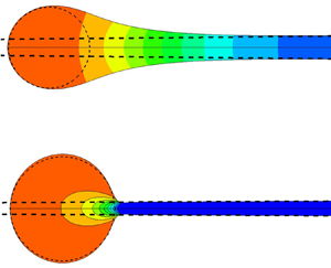
Figure 1. Schematic showing the dimensionless 3-D axisymmetric or 2-D problem of bubbles coalescing in an infinite pool of a power-law liquid. Inset: magnified detail of the liquid film between the coalescing bubbles. (Shaded inset: the computational domain used in the 3-D axisymmetric or 2-D numerical simulations.) The interface representation $z = h(r,t)$ requires the interface to be single valued, and is only used in the analysis relying on the thin-film approximation as described in § 3.

A schematic showing the complete dimensionless problem of two coalescing bubbles, and its reduction to the receding sheet problem is presented in figure 1. Anthony et al. (Reference Anthony, Kamat, Thete, Munro, Lister, Harris and Basaran2017) have performed numerical simulations over the entire problem domain and shown that the results up to $R_{min} \approx 4 \times 10^{-2}$ obtained by solving the full problem are identical to those obtained via a truncated film domain as described here. On account of the validation that has already been presented by Anthony et al. (Reference Anthony, Kamat, Thete, Munro, Lister, Harris and Basaran2017), and also due to the drastic computational savings afforded by use of the truncated domain approach, we obtain all the results to be reported in this work by numerical simulations that are carried out over a truncated domain. Additional details on this procedure are presented in § 4.

2.2. Governing equations

The isothermal, incompressible flow in the liquid film $V$ is governed by the equation of continuity and the Cauchy momentum equation

(2.2a)\begin{gather} \boldsymbol{\nabla} \boldsymbol{\cdot} \boldsymbol{v} = 0 \quad \mbox{in} \ V, \end{gather}

(2.2b)\begin{gather}\frac{\partial \boldsymbol{v}}{\partial t} + \boldsymbol{v}\boldsymbol{\cdot} \boldsymbol{\nabla} \boldsymbol{v} = \boldsymbol{\nabla} \boldsymbol{\cdot} \boldsymbol{\mathsf{T}} \quad \mbox{in}\ V, \end{gather}

where $\boldsymbol {v} = u \boldsymbol {e}_{r} + v \boldsymbol {e}_{z}$ is the fluid velocity, with $u$ and $v$ standing for the radial and axial components of the velocity, and $\boldsymbol{\mathsf{T}}$ is the Cauchy stress tensor given by

(2.3)\begin{equation} \boldsymbol{\mathsf{T}} = -p \boldsymbol{I} + Oh \, \mu \left[ \boldsymbol{\nabla} \boldsymbol{v} + (\boldsymbol{\nabla}\boldsymbol{v})^{\intercal} \right], \end{equation}

where $p$ is the local pressure in the liquid, $Oh = \tilde {\mu }_{0}/(\tilde {\rho } \tilde {R} \tilde {\sigma })^{1/2}$ is the Ohnesorge number and $\mu$ is the local value of the viscosity function. $Oh$ is an important dimensionless number in free-surface flows as it expresses the preponderance of the viscous forces over the inertio-capillary forces in the domain. The dimensionless deformation-rate-dependent viscosity function $\mu$ for a power-law fluid is

(2.4)\begin{equation} \mu= \left| \alpha \dot{\gamma} \right|^{n - 1} \quad \mbox{in}\ V, \end{equation}

where $\alpha ^{-1}$ is the dimensionless characteristic deformation rate, and $\dot {\gamma }$ is twice the second invariant of the rate-of-deformation tensor ${\boldsymbol {\varGamma }}$. The magnitude of the deformation rate, as defined here, is $\dot {\gamma } = [2 ({\boldsymbol {\varGamma }}:{\boldsymbol {\varGamma }})]^{1/2}$ which, in cylindrical coordinates, is given by (see, e.g. Deen Reference Deen2012)

(2.5)\begin{equation} \dot{\gamma} = \left[ 2 \left ( \frac{\partial u}{\partial r}\right )^{2} + 2 \left(\frac{u}{r} \right)^{2} + \left( \frac{\partial u}{\partial z} + \frac{\partial v}{\partial r} \right)^{2} + 2 \left (\frac{\partial v}{\partial z}\right )^{2} \right]^{1/2}. \end{equation}

The free surface $S_{FS}$ separating the liquid – the retracting film – from the gas – the bubbles – is free from tangential stresses as surface tension is constant. Therefore, the traction boundary condition at the free surface is (see, e.g. Scriven Reference Scriven1960; Aris Reference Aris1989; Deen Reference Deen2012)

(2.6)\begin{equation} \boldsymbol{n} \boldsymbol{\cdot} \boldsymbol{\mathsf{T}} = 2\mathcal{H} \boldsymbol{n} \quad \mbox{on}\ S_{FS}, \end{equation}

where $\boldsymbol {n}$ is the unit normal vector pointing outward from the liquid phase, and $2\mathcal {H} = -\nabla _{s}\boldsymbol \cdot \boldsymbol {n}$ is twice the local mean curvature of the free surface $S_{FS}$. Here, $\nabla _{s} = \boldsymbol {\nabla } - \boldsymbol {n}(\boldsymbol {n}\boldsymbol {\cdot }\boldsymbol {\nabla })$ is the surface gradient operator. In addition to the traction boundary condition, the kinematic boundary condition also applies at the interface

(2.7)\begin{equation} \boldsymbol{n} \boldsymbol{\cdot} (\boldsymbol{v} - \boldsymbol{v}_{s}) = 0 \quad \mbox{on}\ S_{FS}, \end{equation}

where $\boldsymbol {v}_{s}$ is the velocity of the free surface in the $(r, z)$-plane.

As the system is symmetric about the $z = 0$ plane ($S_{SYM}$), the flow field there should obey

(2.8a)\begin{gather} \boldsymbol{n} \boldsymbol{\cdot} \boldsymbol{v} = 0 \quad \mbox{on}\ S_{SYM}, \end{gather}

(2.8b)\begin{gather}\boldsymbol{n} \boldsymbol{\cdot} \boldsymbol{\mathsf{T}} \boldsymbol{\cdot} \boldsymbol{t} = 0 \quad \mbox{on}\ S_{SYM}, \end{gather}

where $\boldsymbol {n} = - \boldsymbol {e}_{z}$ is the outward-pointing unit normal vector, and $\boldsymbol {t} = \boldsymbol {e}_{r}$ is the unit tangent vector to $S_{SYM}$.

Far away from the singularity ($r \gg R_{min}$), we expect to observe the far-field flow conditions given by (2.1). These conditions are applied at the boundary $r = R_{trunc}$ where the film is truncated.

2.3. Choice of dimensionless parameters

The non-dimensionalization of the problem as described in § 2.1 results in three important dimensionless parameters that govern the flow: the Ohnesorge number $Oh$, the power-law index $n \le 1$ and the reciprocal of the characteristic deformation rate $\alpha$.

In this work, attention is focused on power-law fluids that are slightly viscous or nearly inviscid when the deformation rate is vanishingly small, i.e. fluids with small values of $\tilde {\mu }_{0}$. Therefore, the study is confined to small Ohnesorge numbers ($Oh \ll 1$). This condition is well met by focusing on situations where, with the exception of a handful of cases, $Oh = 0.01$ and which, as will be demonstrated later on in the paper, allow the observation of virtually the full range of dynamical effects that is possible in the nearly inviscid limit.

The choice of predominantly focusing on $Oh=0.01$ is also reinforced by the fact that the pre-factors obtained by Anthony et al. (Reference Anthony, Kamat, Thete, Munro, Lister, Harris and Basaran2017) at this value of $Oh$ differed from those in the limit of $Oh \to 0$ by about $2.5\,\%$. Consequently, the majority of the results to be presented have been obtained when $Oh = 0.01$ unless it is stated otherwise.

In the equations of this paper, it may be observed that $Oh$ and $\alpha$ appear in combination as $Oh \, \alpha ^{n-1}$. However, as shown in appendix A, it is important to note that the appearance of these two parameters together in this form only occurs as an artifact of employing the power-law limit of the full Carreau model ($\beta \to 0$, $\tilde {\alpha } \tilde {\dot {\gamma }} \gg 1$) in combination with the use of the inertio-capillary time $t_{ic}$ as the characteristic scale for time (as is appropriate when $Oh \ll 1$). In the remainder of the paper, the value of the reciprocal of the dimensionless characteristic deformation rate is held fixed at $\alpha = 1$ in all simulations for ease of comparison with bubble coalescence in a Newtonian fluid of the same $Oh$$(\ll 1)$ as the power-law fluid and in order to observe more clearly trends and variations in the reduced phase space comprised of ($n, R_{min}$).

3.1. Film: thin-film approximation

In the thin-film approximation, the free-surface height is a single-valued function of the radial distance from the axis of symmetry, viz. $z = h(r,t)$, as shown in figure 1, and as the extent of the film in the $r$-direction is much larger than that in the $z$-direction, the radial velocity $u$ and the pressure $p$ are expanded in Taylor series in even powers of $z$ due to symmetry across the plane $z=0$ (the approach presented here follows that used by Eggers (Reference Eggers1993) in the derivation of slender-jet equations and Savva & Bush (Reference Savva and Bush2009) in that of equations governing the retraction of thin sheets in planar and axisymmetric geometries for Newtonian fluids)

(3.1)\begin{gather} u(r, z, t) = u_{0}(r,t) + u_{2}(r,t) z^{2} + {O} (z^{4}) , \end{gather}

(3.2)\begin{gather}p(r, z, t) = p_{0}(r,t) + p_{2}(r,t) z^{2} + {O} (z^{4}) . \end{gather}

In the radial thin-film approximation used here, the axial velocity $v$ can then be determined simply by substituting the expansion for the radial velocity $u$ from (3.1) in the equation of continuity

(3.3)\begin{equation} v(r,z,t) = -\frac{1}{r} \frac{\partial}{\partial r}\left [ r u_0(r,t) \right] z - \frac{1}{r}\frac{\partial}{\partial r} \left [ r u_2(r,t) \right ] \frac{z^3}{3} - {O} (z^{5}). \end{equation}

It should be noted that, to leading order, the axial velocity is of O($z$) and is much smaller than the radial velocity which is of O(1).

These expansions for $u$, $v$ and $p$ are then substituted into the system of (2.2a)–(2.7). Retaining only the O($1$) terms yields a set of evolution equations for the leading-order term in the radial velocity, $u_{0}(r,t)$, and the film thickness $h(r,t)$. Before summarizing those equations, we note that the pressure no longer appears in them because at leading-order it can be expressed through the use of the normal-stress boundary condition in terms of other variables, viz. the radial velocity, velocity gradients and the curvature, as

(3.4)\begin{equation} p_0(r,t) = -2\, Oh\, \mu \frac{1}{r}\frac{\partial}{\partial r} \left [ r u_0(r,t) \right ] - 2\mathcal{H}, \end{equation}

where $\mu$ is the viscosity function at O(1) (see below).

The kinematic boundary condition, combined with the equation of continuity, yields a local mass conservation equation that describes the evolution in time of $h$. Dropping the subscript ‘0’ in the leading-order terms, the 1-D mass balance or mass conservation constraint may be written as

(3.5)\begin{equation} \frac{\partial h}{\partial t} + \frac{1}{r} \frac{\partial }{\partial r} (urh) = 0 , \end{equation}

where $u(r, t)\equiv u_{0}(r,t)$. The 1-D momentum equation describing the evolution in time of $u(r,t) \equiv u_{0}(r, t)$ is

(3.6)\begin{equation} h( u_{t} + u u_{r}) = h\frac{\partial} {\partial r} \left( 2\mathcal{H} \right) + 4 \,{\textit{Oh}} \left\{ \frac{\partial}{\partial r} \left[ \mu h \frac{(r u)_{r}}{r} \right] - \frac{1}{2} \frac{u (\mu h)_{r}}{r} \right\}, \end{equation}

where $2\mathcal {H} = (r h_{r})_{r}/{r}$ to the leading order. Here, and in the text that follows, the subscripts ‘$r$’ and ‘$t$’ denote partial derivatives ${\partial }/{\partial r}$ and ${\partial }/{\partial t}$, respectively, and these notations will henceforward be used interchangeably based on representational convenience. In the 1-D approximation, the viscosity function $\mu$ reduces to

(3.7)\begin{equation} \mu = \left| 2 \alpha \sqrt{\left (\frac{\partial u}{\partial r}\right)^{2} + \left( \frac{u}{r} \right)^{2} + \frac{u}{r} \frac{\partial u}{\partial r}} \right|^{n - 1}. \end{equation}

We note that when $r \gg 1$, the three previous equations reduce to those governing the dynamics of planar films of power-law fluids given in Thete et al. (Reference Thete, Anthony, Basaran and Doshi2015).

The thin-film model is applicable only to the slender sheet that occupies the region $r \ge R_{E}$. In this region, the scales of the forces at play, which are of course those that are due to inertia ($I$), viscous resistance ($V$) and surface tension or capillarity ($C$), can be estimated from (3.6) as

(3.8a)\begin{gather} I \sim h u u_{r} , \end{gather}

(3.8b)\begin{gather}V \sim {\textit{Oh}} \left[ \mu h (u_{r} + u/r) \right]_{r} \sim {\textit{Oh}} \,\alpha^{n-1} h u_{r}^{n-1} u_{rr} , \quad \textrm{and} \end{gather}

(3.8c)\begin{gather}C \sim h h_{rrr} . \end{gather}

Additionally, for the mass conservation constraint (3.5) to be satisfied at the edge of the sheet, the velocity scale must be

(3.9)\begin{equation} u = \frac{\textrm{d} R_{E}}{\textrm{d}t} \sim R_{E}/t \quad \mbox{at} \ r = R_{E} . \end{equation}

To satisfy the matching criterion with the rounded tip at $R=R_{E}$, the thin-film shape function $h$ must equal the maximum height of the tip

(3.10)\begin{equation} h = h_{E} \quad \mbox{at} \ r = R_{E} . \end{equation}

3.2. Tip: force balance

Munro et al. (Reference Munro, Anthony, Basaran and Lister2015) assumed that the film solution terminates at $r = R_{E}$ in a rounded cap of (in-plane) radius $h_{E}$. The large in-plane curvature $1/h_{E}$ of the tip causes a large capillary pressure there and thereby drives the entire flow field within the thin film adjacent to it. The flow that is thereby generated thus gives rise to inertial and viscous forces that affect the overall film shape and other self-similar features of the dynamics in the entire domain. Although an exact solution describing the dynamics in the tip region can be obtained by rigorous asymptotic analysis as has been done by Eggers (Reference Eggers2014) for a retracting thread and Howell et al. (Reference Howell, Scheid and Stone2010) for a spinning sheet, and which can then be matched with the solution in the retracting thin sheet, we follow the heuristic but physically based approach of Munro et al. (Reference Munro, Anthony, Basaran and Lister2015) who approximated the leading-order effects using a generalized force balance $F_{net, tip} = \int _{S_{Tip}} \boldsymbol {n} \boldsymbol {\cdot } \boldsymbol{\mathsf{T}} \,\textrm {d}S$. Munro & Lister (Reference Munro and Lister2018) have rigorously demonstrated the validity of this approach in the creeping flow limit by solving without approximation the Stokes equations in the situation in which the edge of a thin sheet (film) is retracting while the sheet is simultaneously and uniformly being stretched edgewise, i.e. in the direction perpendicular to that of retraction, a problem that is a close analogue of the axisymmetrically growing rim in the bubble coalescence problem analysed in this paper.

The leading-order force balance over a section of the rim is given by

(3.11)\begin{equation} \frac{\textrm{D}u}{\textrm{D}t} \frac{{\rm \pi} h_{E}^{2}}{4} = 1 + h_{E} \left[ 2\mathcal{H} + 2 \,{\textit{Oh}}\, \mu \left( 2\frac{\partial u}{\partial r} + \frac{u}{r} \right) \right]_{r = R_{E}}, \end{equation}

and encapsulates the interplay between the driving capillary force (the first term on the right side) and the two retarding forces – one due to inertia (the term on the left side) and the other to viscosity at $r = R_{E}$ (the term inside the brackets that is multiplied by $Oh$). Equation (3.11) allows estimation of the scales of the principal forces in the tip region as

(3.12a)\begin{gather} I_{tip} \sim h_{E}^{2} u u_{r}, \end{gather}

(3.12b)\begin{gather}V_{tip} \sim {\textit{Oh}} \,\alpha^{n-1} h_{E}u_{r}^{n} \quad \textrm{and} \end{gather}

(3.12c)\begin{gather}C_{tip} \sim 1. \end{gather}

Note that in the estimation of the viscous force $V_{tip}$, we neglect the small capillary contribution to the net visco-capillary resistance ($2\mathcal {H}_{r = R_{E}} \ll 1$).

4.1. Initial condition

Bubble coalescence begins at the exact point in time and space at which the liquid sheet ruptures ($t = 0$, $R_{min} = 0$), but this state is not realizable in a numerical simulation (Anthony, Harris & Basaran Reference Anthony, Harris and Basaran2020) without an a priori knowledge of the full nature of the singularity. Moreover, since the limit of continuum mechanics is approximately 10 nm, simulations have to begin from an initial state in which a small but finite hole or a gas bridge of radius $R_{min}(t)$, where $0< R_{0} \equiv R_{min}(t = 0) \ll 1$, has already formed. In the same vein, we begin with a 2-D shape profile of a perfect circle for the bubble free surface $h(r, 0)$ with a circular cap, to close the curve, at $R_{E} (t=0) = R_{0} + Z_{0}$, where $Z_{0} = R_{0}^{2} = h(R_{E}(0),0)$. Moreover, the simulations are begun with an initially quiescent fluid where the velocity $\boldsymbol {v} = 0$ over the entire domain. Once the simulations start, at extremely early times, the dynamics, on account of being universal, transitions from the initially quiescent state into one that bears no dependence on or retains no imprint of the imposed initial condition. This independence is clearly demonstrated in figure 2 where results from simulations using different values of $R_{0}$, but while holding fixed the dimensionless parameters $Oh$, $\alpha$ and $n$, can be seen to tend towards a universal profile of $R_{min}(t)$ versus $t$ once sufficient time has elapsed and all initial transients have died out. The reader is referred to Anthony et al. (Reference Anthony, Kamat, Thete, Munro, Lister, Harris and Basaran2017) for a more detailed discussion on this subject.

Figure 2. The variation of the minimum neck radius $R_{min}$ with time $t$ when $Oh = 0.01$ and $n = 0.85$ obtained from two simulations with distinct initial conditions: $R_{0} = 10^{-5}$ (green) and $R_0 = 10^{-4}$ (blue). After the initial transients have died out, both cases are seen to follow universal scaling. Here, $Z_{0} = R_{0}^{2}$ in both simulations. The effect of varying the initial half-height of the bridge $Z_{0}$ is discussed in depth by Anthony et al. (Reference Anthony, Kamat, Thete, Munro, Lister, Harris and Basaran2017).

4.2. Truncation point

The reduction of the full problem to that of the truncated film necessitates the imposition of a far-field condition at a radial distance $R_{trunc}$ sufficiently far away from the singularity. Munro et al. (Reference Munro, Anthony, Basaran and Lister2015) and Anthony et al. (Reference Anthony, Kamat, Thete, Munro, Lister, Harris and Basaran2017) show that the flows generated by the retracting tip typically decay by an order of magnitude over a radial distance $\Delta r \propto Oh\, R_{min}$ when $Oh \ll 1$, and over ${\rm \Delta} r \propto R_{min}$ when $Oh \gg 1$. Consequently, stopping our simulations when $R_{min}$ reaches a value of $0.1R_{trunc}$ makes our results independent of the initial value of $R_{trunc}$ as the far-field condition is always satisfied at $r = R_{trunc}$. In this work, all our results have been obtained using $R_{trunc} = 1000 R_{0}$ unless otherwise stated.

4.3. Tracking of scales

To analyse the dynamics of the receding film, we track the dominant scales that have an impact on the overall force balance in the tip and film regions. To do so, we first need to determine the location where the tip and film join ($r = R_{E}$). In the rounded tip, the magnitude of $h_{r} \equiv \partial h/\partial r$ is large except in the vicinity of where the tip merges with the film and where $h_{r} \equiv \partial h/\partial r$ becomes negligible. Moreover, monitoring the value of $h_{r}$ allows us to pinpoint the location of where the radius of the tip is a maximum as when it bulges, which has been shown to occur for $Oh \ll 1$ by Munro et al. (Reference Munro, Anthony, Basaran and Lister2015) and Anthony et al. (Reference Anthony, Kamat, Thete, Munro, Lister, Harris and Basaran2017). In the 2-D simulations, we track the value of the derivative of the axial coordinate $z$ with respect to arclength along the free surface

(4.1)\begin{equation} \partial z/\partial s = \frac{h_{r}}{(1+h_{r}^{2})^{1/2}}, \end{equation}

where $s$ is the arclength measured from the tip ($R_{min}, 0$). At each time step, starting from the tip, we march along the free surface towards the film, and mark the radial position where $\partial z/\partial s$ has dropped from its value of unity at the tip to some small value ($5 \times 10^{-2}$) as the matching point $R_{E}$. The height of the film at this radial location is then set equal to $h_{E}$. The length or radial extent of the tip is denoted by ${\rm \Delta} r_{tip} = R_{E} - R_{min}$. As capillary forces tend to keep the tip ($r < R_{E}$) circular, it is expected based on intuition that ${\rm \Delta} r_{tip} \approx h_{E}$. That this is indeed the case is demonstrated in figure 3(a) which shows for the situation in which $Oh = 0.01$ and $n = 0.85$ that the profiles depicting the evolution in time $t$ of $h_{E}$ and ${\rm \Delta} r_{tip}$ lie on top of each other over a time period that spans five orders of magnitude. Figure 3(b) shows that as a consequence of ${\rm \Delta} r_{tip} \approx h_{E}$, combined with the fact that $h_{E} \ll R_{min}$ (discussed in § 6), the scaling of $R_{min}$ and that of $R_{E}$ with $t$ are indistinguishable. It is important to note that the results depicted in figure 3 justify the ansatz of a rounded tip in the 1-D analysis of Munro et al. (Reference Munro, Anthony, Basaran and Lister2015), i.e. these authors assume that $R_{min} \approx R_{E}$ while reporting the scaling of $R_{E}$ with $t$. Munro & Lister (Reference Munro and Lister2018) have demonstrated through their rigorous analysis the validity of the nearly rounded tip ansatz for the edge of retracting stretched viscous films ($Oh^2 \gg 1$) but not for the nearly inviscid ($Oh \ll 1$) films that are under study in this paper.

Figure 3. Comparison when $Oh = 0.01$ and $n = 0.85$ of the temporal evolution of (a) $h_{E}$ (thick green line) and ${\rm \Delta} r_{tip} = R_{E}-R_{min}$ (thin black line), and (b) $R_{min}$ (thick green line) and $R_{E}$ (thin black line). (a) shows that the tip is indeed circular as its radial and axial extents remain approximately equal, viz. ${\rm \Delta} r_{tip} \approx h_{E}$, during coalescence. Also, as $h_{E} \ll R_{min}$ (see § 6), $R_{min}$ and $R_{E}= R_{min} + {\rm \Delta} r_{tip}$ exhibit the same scaling with respect to time, as shown in (b).

In the rounded tip, we determine the important forces $I_{tip}$, $V_{tip}$ and $C_{tip}$ from their first-principle definitions that involve calculation of either a surface or a volume integral and thereby infer the dominant balance of forces (see § 6). To analyse all the relevant scales that are involved, we track $u$ and $u_{r}$ in the tip at the location $r = (R_{min}+R_{E})/2$ on the symmetry plane ($z = 0$). In what follows, we denote these values by $u_{tip}$ and $u_{r, tip}$ respectively.

In the thin film, we track the maximum absolute values of $u$ and $u_{r}$, and the minimum value of $\mu$ along with their radial locations on the symmetry plane $S_{SYM}$. How the film thickness $h$ scales with time $t$ in the film is determined by monitoring the instantaneous value of $h$ at the location $r = R_{E} + {\rm \Delta} r_{tip}$ to ensure that the evaluation is made outside of the tip but within the compressional boundary layer in the film. To estimate the scales of the velocity gradients, it is important to track the two important length scales $L_{u}$ – the radial distance over which $u$ drops by an order of magnitude from its maximum value at the tip, and $L_{ur}$ – the radial distance from the tip over which $u_{r}$ attains its maximum value. Therefore, we estimate the radial velocity gradients as

(4.2a)\begin{gather} u_{r} \sim u/L_{u}, \quad \textrm{and} \end{gather}

(4.2b)\begin{gather}u_{rr} \sim u_{r} / L_{ur}. \end{gather}

These scale definitions have been used to obtain all the results presented in the following sections.

6.1. Velocity and velocity derivative scaling, and implications for tip forces

Simulations show that in the tip, the radial velocity $u_{tip}$ and its radial derivative $u_{r, tip}$ scale in accordance with the scaling estimates obtained from the mass conservation constraint (3.9), viz. $u_{tip}$ scales as $R_{min}/t \sim R_{min}^{-1}$ and $u_{r, tip}$ scales as $u_{tip}/R_{min} \sim R_{min}^{-2}$. This is demonstrated in figure 5 for the situation in which $Oh=0.01$ and ${\textit {n}} = 0.9$. Based on these scales, we now seek to arrive at a universal scaling law for $h_{E}$ by balancing the dominant forces in the tip (3.12), i.e.

(6.1)\begin{gather} I_{tip} \sim h_E^2 R_{min}^{-3} \end{gather}

(6.2)\begin{gather}V_{tip} \sim Oh \, h_E \, R_{min}^{-2n} \end{gather}

(6.3)\begin{gather}C_{tip} \sim 1. \end{gather}

Figure 5. Simulation results on the scaling of (a) the velocity $u_{tip}$ and (b) the derivative of the velocity $u_{r, tip}$ in the tip with minimum neck radius $R_{min}$ when $Oh = 0.01$ and ${\textit {n}} = 0.9$ (thick green lines/curves). The computed results obey the theoretical scaling predictions that $u_{tip} \sim R_{min}^{-1}$ and $u_{r, tip} \sim R_{min}^{-2}$ (shown as black lines of slopes $-1$ and $-2$ in (a) and (b)).

6.2. Asymptotic tip conditions

The capillary force in the tip $C_{tip}$ which is responsible for driving the coalescence process is balanced by (i) the viscous resistance $V_{tip}$ at $r = R_{E}$, (ii) the inertia of the tip $I_{tip}$ or (iii) a combination of viscous resistance and inertia (see (3.11)). It will be shown below that the latter balance, case (iii) where $C_{tip} \sim V_{tip} \sim I_{tip}$, leads to an inconsistency or impossibility unless $n=3/4$. Therefore, in general, the tip must be predominantly either viscous (case (i) where $C_{tip} \sim V_{tip}$) or inertial (case (ii) where $C_{tip} \sim I_{tip}$).

Case (i): in the viscous tip limit, balancing viscous and capillary forces from (6.2) and (6.3), we arrive at the scaling prediction that

(6.4)\begin{equation} h_{E} \sim \frac {1}{Oh} R_{min}^{2n} \sim R_{min}^{2n} \end{equation}

In their study of bubble coalescence in Newtonian fluids, Munro et al. (Reference Munro, Anthony, Basaran and Lister2015) assumed this balance to always hold, thereby arriving at $h_{E} \sim R_{min}^{2}$ (for $n = 1$). When $n=1$, we find from the new simulations that the dominant balance is indeed between capillary and viscous forces. This is demonstrated by the results obtained when $Oh=0.01$ from the first-principles force-balance calculation that are shown in figure 6(a). We further find in this case where $n=1$ and $Oh=0.01$ that the scaling relation given in (6.4) where $h_E$ varies quadratically with $R_{min}$ is indeed correct for small values of $R_{min}$ as shown in figure 7(a). When the liquid surrounding the two bubbles is a power-law fluid of $n=0.9$ and $Oh=0.05$, figure 6(b) shows that the balance is once again between viscous and capillary forces. Furthermore, the simulations in this case (figure 7b) predict that $h_E \sim R_{min}^{1.8}$, in accord with (6.4).

Figure 6. Variation with the minimum hole radius $R_{min}$ of the forces in the tip that have been determined from first-principle calculations when: (a) $Oh = 0.01$, $n=1$, (b) $Oh = 0.05$, $n=0.9$ and (c) $Oh = 0.01$, $n = 0.8$. The different forces are colour coded as: $I_{tip}$, blue; $V_{tip}$, red; and $C_{tip}$, black. The force balance demonstrates the viscous tip condition $V_{tip}\sim C_{tip}$ in cases (a,b), and the inertial tip condition $I_{tip}\sim C_{tip}$ in case (c).

Figure 7. Computed variation of (half) film thickness $h$ with $R_{min}$ determined from simulations when: (a) $Oh=0.01$, $n=1$; (b) $Oh=0.05$, $n=0.9$; (c) $Oh=0.01$, $n=0.9$; and (d) $Oh=0.01$, $n=0.8$. The thick coloured lines are the simulation results and the thin black lines, as indicated, are lines of slope $2n$ or 3/2. For the cases with $Oh = 0.01$ (a,c,d), over the range of values of $R_{min}$ shown, the scaling exponent in the relationship between $h$ and $R_{min}$ changes from 2 in the Newtonian case, (a), to 3/2 in the power-law cases, (c,d), as $n$ is reduced from its Newtonian value of 1, indicating that the importance of inertia in the tip rises as $n$ falls.

Case (ii): in the inertial tip limit, balancing inertial and capillary forces from (6.1) and (6.3), we arrive at the scaling prediction that

(6.5)\begin{equation} h_{E} \sim R_{min}^{3/2} .\end{equation}

Simulations for a power-law fluid of $n=0.8$ when $Oh=0.01$ as highlighted by the results of first-principles force-balance calculations that are shown in figure 6(c) indicate that the balance is between inertial and capillary forces. Moreover, scaling results depicting the variation of $h_E$ with $R_{min}$ obtained from simulations for two different power-law fluids of different values of the power-law exponent of $n=0.9$ and $n=0.8$ but at the same value of $Oh=0.01$ shown in figures 7(c) and 7(d) indicate that the exponent in the scaling law relating $h_{E}$ to $R_{min}$ equals the inertial exponent of 3/2, in accordance with (6.5).

Therefore, the dominant balance of forces in the tip in the immediate aftermath of the coalescence singularity is always between viscous and capillary forces when the liquid surrounding the bubbles is Newtonian but it may be between either viscous and capillary forces or inertial and capillary forces when the liquid is a power-law fluid. The maximum height of the tip $h_E$, on the other hand, has been found to scale at early times as the minimum radius $R_{min}$ raised to the $2n$ power when the tip is viscous but $R_{min}$ raised to the 3/2 power when the tip is inertial. However, the differences that are observed in the dominant balance of forces and the values of the scaling exponents relating $h_{E}$ to $R_{min}$ for different values of $n$ and $Oh$ at early times tell only a part of the complete story. We return to these matters below after we have discussed case (iii) and the implications of the scaling of $h_E$ to the scaling of film thickness.

Case (iii): if all three forces are important, it follows from comparing (6.4) and (6.5) that this can only happen in the special situation when $n=3/4$. We refer to this special case as the inertial–viscous limit.

Combining the result on the scaling of $h_{E}$ with the tip film matching condition (3.10) and using the self-similarity ansatz in the film, we have thus uncovered the universal, self-similar scaling for (half) the film thickness $h$. In the simulations, we measure $h$ at $r = R_{E} + {\rm \Delta} r_{tip}$, where ${\rm \Delta} r_{tip} = R_{E} - R_{min}$, to ensure that the measurement always remains outside of but also adjacent to the tip. Figure 8 shows the computed scaling of $h$ with $R_{min}$ obtained from simulations for the case of a Newtonian fluid ($n = 1$) of $Oh = 0.01$. These results clearly show that $h$ undergoes a scaling transition from the viscous tip scaling where $h \sim R_{min}^{2}$ to the inertial tip scaling where $h \sim R_{min}^{3/2}$ when the minimum neck radius reaches a critical value of $R_{min} \approx 4 \times 10^{-4}$. We will next discuss the cause of this transition, and similar ones that occur for power-law fluids, and theoretically predict the transition point(s).

Figure 8. Simulation results showing the computed variation of (half) film thickness $h$ with hole radius $R_{min}$ when $Oh = 0.01$ and $n = 1$. The results show that a transition takes place in the dynamics as $R_{min}$ increases from where the tip is viscous (with a scaling exponent of 2) to one where the tip is inertial (with a scaling exponent of 3/2). In the figure, results from three different simulations (indicated by the coloured data points) starting with different initial hole radii of $R_{0} = 10^{-6}$, $10^{-5}$ and $10^{-4}$ have been superimposed to cover a wide range of $R_{min}$ as discussed in Anthony et al. (Reference Anthony, Kamat, Thete, Munro, Lister, Harris and Basaran2017). Straight lines of slope 2 and 3/2 are shown to highlight where the tip dynamics is viscous and where it is inertial, and to emphasize that the transition between them occurs when $R_{min} \approx 4 \times 10^{-4}$.

6.3. Magnitudes of forces, regimes and transition points

First, it is instructive to calculate the scaling of the inertial force in the viscous tip limit that is by assumption negligible in this limit. From (6.1), it follows that

(6.6)\begin{equation} I_{tip} \sim \frac {1}{Oh^2}\, R_{min}^{4n-3} .\end{equation}

Therefore, as $R_{min} \rightarrow 0$ or in the immediate aftermath of the singularity, we see that inertia is negligible and the tip is viscous provided that $3/4 < n \le 1$.

Next, we determine the scaling of the viscous force in the inertial limit that is now by assumption negligible in this limit. From (6.2), it follows that

(6.7)\begin{equation} V_{tip} \sim Oh \, R_{min}^{(3-4n)/2} .\end{equation}

Therefore, as $R_{min} \rightarrow 0$ or in the immediate aftermath of the singularity, we see that viscous force is negligible provided that $n < 3/4$.

However, we also note from (6.6) that inertia can become important as $R_{min}$ or time increases when $3/4 < n \le 1$ and that according to (6.6), $I_{tip} \to \infty$ as $R_{min} \to 0$ when $n<3/4$. We further note from (6.7) that viscous force can become important as $R_{min}$ or time increases when $3/4 < n$ and that according to (6.7), $V_{tip} \to \infty$ as $R_{min} \to 0$ when $3/4 < n \le 1$. Therefore, not only the assumption that the inertial or viscous force always be small for all times or all values of $n$ is incorrect, but the possibility exists for a change of scaling or regime as coalescence proceeds.

To determine any transitions, we note that since $V_{tip} \sim h_E \,Oh\, R_{min}^{-2n}$ and $I_{tip} \sim h_E^2 R_{min}^{-3}$, when these forces become comparable and transition from a viscous (inertial) tip to an inertial (viscous) tip regime is possible

(6.8)\begin{equation} h_E \sim Oh \,R_{min}^{3-2n}. \end{equation}

Thus, when $3/4 < n \le 1$, coalescence begins in the viscous tip regime. However, as time advances and hole radius grows, inertia can eventually become significant and comparable to viscous force. The point of transition from the viscous tip regime to the inertial tip regime can then be determined by substituting the viscous tip scaling law $h_E \sim R_{min}^{2n}/Oh$ into (6.8)

(6.9)\begin{equation} R_{min} \sim Oh^{2/(4n-3)} \quad {\text{(viscous to inertial transition)}}. \end{equation}

Such a transition is clearly possible as the value of the critical minimum radius predicted by (6.9) is smaller than one since $Oh<1$ and $n>3/4$.

If, however, $0 < n < 3/4$, coalescence begins in the inertial tip regime. As time advances and hole radius grows, viscous force can grow and eventually may become comparable to inertial force. The point of transition from the inertial tip to the viscous tip regime can be determined by substituting the inertial tip scaling law $h_E \sim R_{min}^{3/2}$ into (6.8)

(6.10)\begin{equation} R_{min} \sim Oh^{2/(4n-3)} \quad {\text{(inertial to viscous transition)}}. \end{equation}

Although (6.10) is identical to (6.9), a transition from the inertial tip to the viscous tip regime is impossible because the minimum radius (whose value is always much smaller than one) at the transition predicted by (6.10) would be larger than one since $Oh<1$ and $n<3/4$.

A more detailed analysis and calculation can be carried out to estimate the prefactor in the expressions for the critical value of the minimum radius for transition and yields

(6.11)\begin{equation} R_{min}^{tip} \approx 1.807 \left[ \frac{3^{(n-1)/2} \, 4 \, Oh\, \alpha^{n-1}}{\sqrt{1.807 {\rm \pi}}} \right]^{2/(4n - 3)}. \end{equation}

Therefore, when $3/4 < n \le 1$, coalescence begins in the viscous tip regime. However, as the hole radius grows, a transition can take place from the viscous tip to the inertial tip regime.

For $n = 1$, (6.9) shows that the value of the minimum radius at the transition scales as $Oh^2$ and (6.11) predicts the point of transition to be $R_{min} \approx 5.09 \, Oh^{2}$. When $Oh = 0.01$, figure 8 shows that the minimum radius for the transition to occur determined from simulations is $R_{min} \approx 4 \times 10^{-4}$, a value that is close to that given by the theoretical prediction from (6.11). However, as we reduce $n$, the value of $R_{min}^{tip}$ drops precipitously below numerically accessible values. For example, when $n=0.8$ and $Oh = 0.01$, the tip transition is estimated or predicted to take place at $R_{min} \approx 10^{-18}$ which, in a real system, would lie well below the continuum limit. However, if the power-law index and the Ohnesorge number are both increased so that $n = 0.9$ and $Oh=0.05$, the value of the minimum radius $R_{min}^{tip}$ for transition increases to $3.9 \times 10^{-4}$ which is sufficiently large so that viscous tip scaling (6.4) can be observed in the simulations as shown in figure 7(b).

This analysis also helps to completely rationalize many of the main results reported in figures 6 and 7 when $Oh=0.01$. For the Newtonian case ($n=1$), the values of the minimum radius are sufficiently small in these figures so that the tip is viscous such that $V_{tip} \sim C_{tip} \gg I_{tip}$ and $h_E \sim R_{min}^2$. Moreover, as expected, we see that $V_{tip}$ is falling and that $I_{tip}$ is rising as $R_{min}$ is increasing in figure 6(a). When $n=0.8$ and 0.9, the values of the transition radii are approximately $10^{-18}$ and $10^{-6}$, respectively. Thus, the dynamics has already transitioned into the inertial regime where $I_{tip} \sim C_{tip} \gg V_{tip}$ and $h_E \sim R_{min}^{3/2}$, as shown in figure 6(c) and figures 7(c) and 7(d) where results are plotted for values of $R_{min} \ge 10^{-5}$.

Additionally, (6.11) suggests that, as we move towards $n = 3/4$, the transition point will asymptotically tend to $R_{min} \rightarrow 0$ where $h$ scales as $R_{min}^{3/2}$. Such a criticality has also been observed for power-law fluids with $Oh \ll 1$ in the context of other singularities that arise during thread breakup (Doshi et al. Reference Doshi, Suryo, Yildirim, McKinley and Basaran2003; Suryo & Basaran Reference Suryo and Basaran2006) and film rupture (Thete et al. Reference Thete, Anthony, Basaran and Doshi2015) where, as in the present problem, the flow behaviour transitions from that of a slightly viscous state to one representing a purely inviscid state.

Furthermore, when $0 < n < 3/4$, coalescence begins in the inertial tip regime. However, as the hole radius grows, the tip continues to remain inertial as a transition from an inertial tip to a viscous tip regime is not possible. Once again, a similar outcome has also been observed in the previously cited studies on thread breakup and film rupture. It would be appropriate to summarize in a phase diagram (figure 17) the physics that has been uncovered in this section on the dynamics that occurs in the immediate aftermath of the coalescence singularity and any transitions that may arise between dynamical regimes as time increases. As it will be shown in the next couple of sections, however, it proves advantageous to postpone the presentation of such a phase diagram until after an analysis has been carried out of the dynamics in the thin film (sheet).

8.1. Relation between $L$ and $2h_{E}$

Figure 11 makes plain that the self-similar flow in the film is nearly unidirectional in nature and has a characteristic length scale which is larger than twice the tip height ($L > 2h_{E}$). This flow regime within the film is realized regardless of which of the tip conditions discussed in § 6 applies. Therefore, the scaling $L \sim R_{min}^{2/n -1}$ holds true with either a viscous tip, for which $h_{E} \sim R_{min}^{2n}$, or an inertial tip, for which $h_{E} \sim R_{min}^{3/2}$. However, as $n$ is lowered, the argument that has just been presented may be violated and this is a point that we return to below.

Figure 12(a) shows the computed variation of $L$ (hollow green squares) and $2h_{E}$ (solid blue line) with $R_{min}$ for the situation in which $Oh = 0.01$ and $n = 0.85$. The simulation results show that at small times, $L$ scales as $R_{min}^{2/n - 1}$ (dashed red line). However, the simulations also show that near a critical value of the minimum hole radius, and at which point $L \approx 2 h_E$, a transition takes place and thereafter the dynamical evolution of $L$ clearly deviates from the dashed line marked as $R_{min}^{2/n - 1}$ and instead follows the solid line marked as $L = 2 h_E$. Therefore, the instant where $L \approx 2h_{E}$ signals the departure of the dynamics from the self-similar description given in § 7 and its transition to a new regime where $L = 2h_{E} \sim R_{min}^{3/2}$.

Figure 12. Simulation results showing the transition from the self-similar regime to Keller's regime when $Oh = 0.01$ and $n = 0.85$. (a) Variation of $L$ with $h_E$. $L$ (green hollow squares) initially scales as $R_{min}^{2/n - 1}$ (red dashed line) and is larger than $2h_E$. Once $L=2h_E$, $L$ undergoes a transition such that thereafter $L \equiv 2h_E$ where $2 h_{E} \sim R_{min}^{3/2}$ (solid blue line). Flows near the tip (b) before and (c) after the transition to Keller's regime. Both the radial and the axial coordinates have been normalized as discussed in the text.

From the profiles shown in figure 11, it is clear that the tip and the part of the film within a radial distance $L$ from it bulge out from continual accumulation of fluid. As the bulging gets more pronounced, fluid is preferentially driven toward this region due to the negative in-plane curvature of the free surface near the tail end (hereafter referred to as the ‘tail’) of the tip as it connects to the thin film downstream. This low-pressure zone is clearly visible near the tail in figure 12(b) which presents a snapshot of the dynamics before the $L = 2h_{E}$ condition is met.

Indeed, the tail region connects the highest point of the tip (where $h = h_E$) to the thin-film region (where $h \sim r^2$) over the radial distance $L - {\rm \Delta} r_{tip}$ ($\approx L - h_E$; see figure 3a). The magnitude of the negative in-plane curvature in this region therefore grows as $h_{E}$ continues to rise faster than $L$ for times leading up to the transition point.

Once $L \approx 2h_{E}$, the profile of the bulge, i.e. the tip plus the tail, becomes nearly a perfect circle, and this region is hereafter referred to as the blob. The corner-like profile of the interface at the location where the blob joins the thin film guarantees the continued existence of a large negative in-plane curvature in that locale. The negative Laplace (capillary) pressures generated there are sufficiently large in magnitude that they cause fluid to flow from the film toward the corner. Thus, as shown in figure 12(c), where $L$ has already undergone the critical transition to thereafter equal $2 h_{E}$, the flow in the bulge toward increasing $r$ and the flow in the film in the direction of decreasing $r$ collide, leading to the formation of a stagnation zone and completely arresting the flow of liquid from exiting the bulge.

We show in figure 13 the flow field within the tip and a portion of the film at an instant in time in a situation where this transition has taken place to further highlight the difference in the flow fields before (cf. figure 11) and after this transition. Moreover, we note that we return below again to this important issue once we have had the chance to discuss certain physical ramifications of this transition. It is noteworthy that once the transition occurs, the stagnation zone flows ensure that the $L = 2 h_{E}$ condition is never overshot, i.e. $L$ never falls below $2h_E$, and prevent overturning of the free surface and/or rupturing of the film beyond this point.

Figure 13. Instantaneous profiles of flow fields within the tip and a portion of the film near the tip for the situation in which $Oh = 0.01$ and $n = 0.8$ at the instant when $R_{min} = 1.021 \times 10^{-3}$. Here, the horizontal coordinate or the abscissa represents the radial distance from the tip $r - R_{min}$. The instantaneous streamlines have been marked with black arrows to indicate the direction of flow and overlaid on top of the contours of the radial velocity $u$ (values of the coloured contours of $u$ are shown in the legend). Inset: a zoomed in view of the region where the tip and the film join and the interface has a corner-like appearance. Clearly visible are the stagnation zone underneath the corner and the weak recirculations in the film.

8.2. Keller's limit

Reassuringly, the formation of the stagnation zone as has just been demonstrated provides strong justification for and is reminiscent of the assumption that Keller (Reference Keller1983) made in his now famous analysis of retraction of edges or filaments of inviscid fluids. Keller assumed that at any time $t'$, all the liquid that is initially contained in the film over $0 < r < R_{min}(t')$ at the onset of the space–time singularity ($t = 0$) accumulates in a growing toroidal ring of instantaneous radius $R_{min}(t')$. For this to occur, the fluid exiting the blob must be arrested, viz. this physical effect may only be produced by a stagnation zone that is created by the formation of the low-pressure corner region where the blob joins the thin film. Based on this assumption, Keller conducted a simple force balance by equating the driving capillary force on the blob to its inertia (in a way that is similar to the inertial tip condition discussed in § 6) to obtain the radial scaling

(8.1)\begin{equation} R_{min} = (32/3)^{1/4}\, t^{1/2}, \end{equation}

where $(32/3)^{1/4} \approx 1.807$, the same prefactor as that obtained for bubble coalescence in nearly inviscid liquids ($Oh \ll 1$) of Newtonian fluids (Munro et al. Reference Munro, Anthony, Basaran and Lister2015; Anthony et al. Reference Anthony, Kamat, Thete, Munro, Lister, Harris and Basaran2017) and power-law fluids (this work).

Although not done by Keller, it is possible to obtain the scaling for $h_{E}$ by equating the mass gathered by the blob with the volume of a toroidal ring with a circular cross-section of radius $h_{E}$ (assuming that the cross-section of the blob in the $(r,z)$-plane is perfectly circular)

(8.2)\begin{equation} \int\limits_{0}^{R_{min}(t)} 2{\rm \pi} r[2h_{0}(r)]\,\mathrm{d} r = 2{\rm \pi} \, R_{min}(t)[{\rm \pi} h_{E}^{2}(t)], \end{equation}

where $h_{0}(r) \approx r^{2}$ is the profile of half the film height at $t = 0$. Evaluation of the integral in the previous equation yields the required expression for $h_{E}(t)$

(8.3)\begin{equation} h_{E} = \frac{1}{2\,\sqrt{\rm \pi}}\, R_{min}^{3/2}. \end{equation}

This finding leads to an expected conclusion: once the tip has transitioned to Keller's regime – from a state where either the viscous tip condition or the inertial tip condition held – the tip thereafter either assumes or retains its inertial character, respectively.

We call the condition where $L = 2h_{E}$ Keller's limit as it is directly linked to the breakdown of the nearly unidirectional flow that occurs after the formation of a perfectly circular blob which joins the outer film, giving rise to a corner at the matching location which results in the creation of a stagnation zone (figure 12c). We show in figure 14 simulation results that clearly differentiate the dynamics before and after Keller's insightful assumption is met.

Figure 14. Contrast between the dynamics of bubble coalescence before (a) and after (b) Keller's limit. The contours represent the normalized radial velocity of the fluid in the reference frame of the tip, $u'=u/U_{tip} - 1$. In both cases, the dashed lines represent the film shape at $t = 0$ and the dash-dot lines correspond to the plane of symmetry $z=0$. During the period of the dynamics prior to Keller's limit (a), it can be seen that not all of the film swept up by the tip (contained in $r < R_{min}(t)$) accumulates in the tip (shown as a dashed circle); a portion of that volume instead accumulates in the compressional boundary layer whose height in the $z$-direction is larger than the downstream film thickness. In the aftermath of the Keller limit (b), the fluid swept up by the tip has now fully accumulated in the tip, thereby exactly satisfying Keller's original assumption. In the latter case (b), the incorporation of the film into the tip also occurs at a speed equal to that of the tip, i.e. $u' = -1$ where the film meets the tip. This is made possible by the stagnation zone that is set up at the corner connecting the tip to the film where the radial velocity now equals zero ($u=0$), a condition that is not satisfied prior to Keller's limit as can clearly be seen in (a). As the stagnation zone persists after it forms, its persistence ensures that beyond Keller's limit, Keller's assumption will continue to remain satisfied for any arbitrary time period $t_1$ to $t_2 > t_1$ during the remainder of the coalescence process.

Given how $L$ varies with $R_{min}$ from (7.2) and equating $L$ with twice $h_E$ obtained from (8.3) yields that the transition value of the minimum radius should scale as $Oh^{2/(5n-4)}$. To be able to predict this limit more quantitatively, we let $\psi (n)$ be the prefactor associated with the scaling for $L$ (7.2) and repeat the procedure that has just been described to deduce that the critical value of $R_{min}$ is given by

(8.4)\begin{equation} R_{min}^{KI} \approx \left( \psi(n) \sqrt{\rm \pi} \right)^{2n/(5n - 4)} \alpha^{2(n-1)/(5n - 4)} \,Oh^{2/(5n - 4)} ,\end{equation}

where the transition to Keller's regime will take place with an inertial tip. The values of $\psi (n)$ and $R_{min}^{KI}$ obtained directly from numerical simulations when $Oh = 0.01$ are listed in table 1. The value of $R_{min}^{KI}$ given in the table for $n = 0.85$, $1.02 \times 10^{-2}$, is in excellent agreement with our simulation results shown in figure 12(a) where the value of the minimum radius for transition from the initial self-similar regime to Keller's regime is shown to be $1.02 \times 10^{-2}$.

Table 1. Values of the prefactor for $L$ scaling ($\psi (n)$) and transition points – hole radius at which a transition occurs from a viscous tip to an inertial tip ($R_{min}^{tip}$), an inertial tip to Keller's limit ($R_{min}^{KI}$) and a viscous tip to Keller's limit ($R_{min}^{KV}$) – when $Oh = 0.01$ for different values of the power-law index $n$ obtained from 2-D simulations.

Table 1 also lists $R_{min}^{KV}$ which is the value of the minimum hole radius where a system will undergo the same type of transition as that just discussed albeit from a viscous tip for which $h_{E} \sim R_{min}^{2n}/Oh$. Carrying out the same sort of balance as that in the previous paragraph yields

(8.5)\begin{equation} R_{min}^{KV} \approx \left( \frac{ \psi(n) \, 1.807^{2n} \, \alpha^{(n^{2} - 1)/n}}{2 \cdot 3^{(1-n)/2}} \right)^{n/(2n^{2} + n - 2)}Oh^{(n+1)/(2n^{2}+n-2)}. \end{equation}

Transition into Keller's regime directly from the viscous tip condition is possible only when $R_{min}^{KV} < R_{min}^{tip}$. From the values of the minimum hole radii for transitions that are listed in table 1, it is clear that the tip transitions from viscous to inertial before Keller's limit is reached for all of the cases listed except for the one when $Oh=0.01$ and $n=0.8$. However, as shown in the table, this transition from a viscous tip to Keller's regime can only occur in this case when the minimum radius $R_{min} (= R_{min}^{KV}) = 1.08\times 10^{-22}$, a value that is orders of magnitude below the continuum limit. The values of $R_{min}^{KV}$ and $R_{min}^{tip}$ given in table 1 for the situation in which $Oh=0.01$ and $n=0.8$ can be extrapolated to situations when $n=0.85$ and $0.9$ to determine the values of $Oh$ that are needed to observe a direct transition from a viscous tip to Keller's limit. By way of example, for the particular case of $n=0.9$, comparison of the relative values of $R_{min}^{tip}$ and $R_{min}^{KV}$ reveals that entrance into Keller's regime directly from the viscous tip condition, i.e. $R_{min}^{KV} < R_{min}^{tip}$, is only possible at extremely small values of both $R_{min}$ (${\lesssim }{O}(10^{-15})$) and $Oh$ (${\lesssim } {O}(10^{-5})$). Consequently, such direct transitions from a viscous tip to Keller's regime are both rare over the parameter space and difficult to observe numerically.

In the Newtonian limit ($n = 1$), it can be shown that $\psi (n)$ has a weak dependence on $Oh$: its value rises from 10.45 (see table 1) when $Oh = 0.01$ to approximately 13.45 when $Oh$ is reduced to 0.003. Considering this range of $\psi$, the critical values of the minimum hole radius for transitions are

(8.6a)\begin{gather} R_{min}^{tip} \approx 5.09\, Oh^{2}, \end{gather}

(8.6b)\begin{gather}R_{min}^{KV} \approx (19.51 \pm 2.45) \, Oh^{2}, \quad \textrm{and} \end{gather}

(8.6c)\begin{gather}R_{min}^{KI} \approx 300 (1.52 \pm 0.38) \, Oh^{2}. \end{gather}

Comparison of the values of the prefactors make plain that when $0 < Oh \ll 1$, bubble coalescence in a Newtonian liquid will exhibit only two transitions: the tip transition from viscous to inertial (8.6a) which would then be followed by the breakdown of unidirectionality as the system transitions into Keller's limit (8.6c).

8.3. Lowering the power-law index $n$

When the power-law index $n$ is lowered from its Newtonian value of 1 to 0.8, the simulations clearly show that $L$ scales as $R_{min}^{2/n - 1}$ (7.2) in all cases (see figure 9). When $n = 0.8$, the exponent $2/n - 1 = 3/2$ is identical to the inertial tip scaling exponent for $h_{E}$ (8.3). Moreover, from the value of $\psi (0.8)$ given in table 1, one can show that the pre-factor for $L$ ($\psi (0.8)\, Oh^{1/0.8} = 0.55$) is approximately twice that of $h_{E}$ ($1/(2\sqrt {{\rm \pi} }) = 0.28$), thereby indicating that the dynamics when $n = 0.8$ always lies in Keller's regime where $L = 2h_{E}$.

Figure 15 shows the $L$ scaling obtained from simulations for the situations in which $n = 0.7$, $0.75$ and $0.8$ when $Oh = 0.01$. Also shown in the figure is the solid black line representing the relationship $L = 2 h_{E}$ as derived from Keller's assumption (8.3). Figure 15 makes it clear that cases for which $n \le 0.8$ lie in Keller's regime where $L \sim R_{min}^{3/2}$, thereby making $n = 0.8$ the critical value of the power-law index above which self-similar film solutions (as detailed in § 7) exist. Therefore, for $n \le 0.8$ when $Oh=0.01$, self-similar film solutions do not exist and the hole grows following Keller's solution during the entire period of its evolution.

Figure 15. Simulation results showing the variation of $L_u \equiv L$ with $R_{min}$ when $Oh = 0.01$ for $n = 0.7$ (orange squares), $0.75$ (purple squares) and $0.8$ (red squares). The data make plain that the scaling in each case follows Keller's scaling of $R_{min}^{3/2}$ (black line).

Although figure 15 shows the exponent in the scaling law for $L$ to equal Keller's value of 3/2 ($L \sim h_{E}$), it is worth noting that for the situations in which $n = 0.7$ and $0.75$, $L > 2 h_{E}$. The reason for this inequality is made clear by figure 16 which shows the shape of the tip and that of the film near the tip along with the streamlines and contours of the viscosity function $\mu$ within them for the situation in which $n = 0.7$ and $Oh = 0.01$. Here, we see that the blob is no longer a perfect circle: it is instead elongated radially and both the tip and the film display signs of capillary waves along their interfaces. Based on the viscosity contours, we may conclude that due to a drastically reduced viscous character, the blob is unable to sustain its inertia while maintaining a circular cross-section. The stagnation flows near the corner formed at the intersection between the blob and the film indicate that despite the inequality between $L$ and $2h_{E}$, this case nevertheless does indeed satisfy the key assumption on which Keller's model is based.

Figure 16. Instantaneous profiles of and flow fields within the tip and a portion of the film near the tip when $R_{min} \approx 1.35 \times 10^{-4}$ for the situation in which $Oh = 0.01$ and $n = 0.7$. Viscosity contours are shown in the upper half of the receding tip/filament while the instantaneous streamlines, which have been marked with black arrows to indicate the direction of flow, are shown in the bottom half. Inset: a zoomed-in view of the region where the tip and the film join shows the noticeable corner region characteristic of the Keller regime. Clearly visible here are the stagnation flows in the film and the capillary waves along the free surface the amplitudes of which decrease with radial distance $r$.

9.1. Scaling of the hole radius $R_{min}$ with time

A significant outcome of the 2-D simulations is that they have shown unequivocally that when $Oh \ll 1$, the scaling with time of the instantaneous value of the minimum hole radius $R_{min} = 1.807 \, t^{1/2}$ holds regardless of the value of the power-law index $n \le 1$. Despite its significance, this result is not surprising as this scaling law had already been shown to be true for both inviscid (Keller Reference Keller1983) and nearly inviscid (Munro et al. Reference Munro, Anthony, Basaran and Lister2015; Anthony et al. Reference Anthony, Kamat, Thete, Munro, Lister, Harris and Basaran2017) fluids in the Newtonian limit ($n = 1$). As the systematic reduction of ${\textit {n}}$ results in further lowering of the viscosity of the receding film, imparting a power-law character on the outer liquid tends to enhance its inviscid-like character and makes the cardinal feature of the dynamics, i.e. the scaling of $R_{min}$ with time $t$, but not all of its other features, indistinguishable from that of an inviscid fluid.

9.2. The rounded tip

The tip condition has been shown to be of critical importance in determining the scaling for (half) the film thickness $h$. By contrast, Munro et al. (Reference Munro, Anthony, Basaran and Lister2015) carried out their scaling analysis with the a priori assumption of a viscous tip, thereby neglecting the tip inertia. In this paper, it has been shown that the viscous tip condition is not sustained indefinitely throughout coalescence but that the dynamics undergoes a transition to an inertial tip condition when the value of the hole radius $R_{min} \approx R_{min}^{tip}$. Results of numerical simulations performed for $n > 3/4$ have been shown to be in excellent agreement with this prediction. It has further been shown in this paper that the tip exhibits a reversal in character for $n < 3/4$ where it is inertial at the singularity. It is theoretically possible that an inertial tip should undergo a transition to a viscous tip when $R_{min} \approx R_{min}^{tip}$ (6.11). However, it has been shown that in the limit of $Oh \ll 1$ and for $n < 3/4$, the transition point $R_{min}^{tip}>1$ and hence such a transition cannot occur during the course of coalescence. Therefore, the viscous tip condition is never encountered when $Oh < 1$ for $n < 3/4$.

9.3. Transition to the truly inviscid regime of bubble coalescence

The dominant length scale $L$ in the thin film, identified from simulations, was used to estimate radial velocity gradients in the domain. As in the Newtonian case, a balance between inertial and viscous forces, i.e. an inertio-viscous balance, is also possible in a power-law film which, in turn, yielded the scaling $L \sim R_{min}^{2/n - 1}$. This scaling, as well as the dominant balance of forces, was confirmed by our simulations a posteriori for $0.8 \le n \le 1$ when $Oh = 0.01$. Simulations further showed a transition from the latter scaling to one where $L \approx 2h_{E}$.

Careful scrutiny of the 2-D flows near the time of the previously discussed transition point led us to conclude that this is a geometrical limit caused by the interface adopting a corner-like profile at the junction of the tip and the circular tip or blob, and where the pressure is severely lowered on account of the large negative planar curvature that exists in that locale. The low-pressure zone underneath the corner gives rise to a stagnation zone thereby preventing fluid from exiting the growing blob – a condition necessary for satisfying Keller's assumption – as well as disrupting the purely unidirectional nature of the self-similar flow in the film – a fact that is readily appreciated by the recirculations that are visible in the film.

In this paper, this transition is termed Keller's limit. Its point of occurrence was theoretically predicted based on the inertial tip condition ($R_{min}^{KI}$) as well as the viscous tip condition ($R_{min}^{KV}$). The former limit was shown to be significantly more common across the parameter space as well as lying within numerically observable ranges of parameter values. The latter limit, on the other hand, could be observed before the dynamics could undergo a transition at $R_{min}^{tip}$ only if $Oh$ and $R_{min}$ could take on unrealistically small values. For example, for a fluid of $n=0.9$, the Ohnesorge number $Oh$ would have to be O($10^{-5}$) and the value of the minimum radius $R_{min}$ would have to be of O($10^{-15}$) for this limit to arise. It was also shown here that a direct transition from a viscous tip to Keller's regime (as hinted by Munro et al. (Reference Munro, Anthony, Basaran and Lister2015)) cannot theoretically occur in the Newtonian limit ($n = 1$) as the tip would instead transition to being inertial before such a transition could take place, viz. $R_{min}^{tip} \ll R_{min}^{KV}$.

Upon further lowering of the power-law index, it was shown that Keller's assumption remains satisfied throughout the coalescence process when $n$ lies below 0.8. Such dynamics entails that the scaling relations $R_{min} = 1.807\, t^{1/2}$, $h_{E} \sim R_{min}^{3/2}$ and $L \sim h_{E}$ hold for all times when $n < 0.8$. Theoretically, however, it is known that when $0.75 < n \le 0.8$, the tip is viscous in the immediate aftermath of the singularity or as $R_{min} \to 0$. From the functional form of $R_{min}^{KV}$, it is readily seen that this quantity tends to zero when $n \approx 0.78$. Therefore, when $n \,\widetilde{<}\, 0.78$, a direct transition from a viscous tip to Keller's limit cannot occur. Thus, for $0.75 < n \,\widetilde{<}\, 0.78$, the tip first transitions from viscous to inertial at a value of the minimum hole radius given by $R_{min} = R_{min}^{tip}$. However, as soon as the tip is inertial, Keller's assumption is satisfied (for $n = 0.8$, $R_{min}^{KI} \to 0)$. Thus, transition to Keller's limit effectively occurs when $R_{min} = R_{min}^{tip}$. On the other hand, for $0.78 \,\widetilde{<}\, n \le 0.8$, because $R_{min}^{KV} > 0$, one of the following two transitions can occur. First, there can be a transition from a viscous tip to Keller's limit when $R_{min} = R_{min}^{KV}$. Alternatively, there can be a transition from a viscous tip to an inertial tip when $R_{min} = R_{min}^{tip}$. In the latter case, Keller's assumption is satisfied as soon as the tip becomes inertial. Therefore, when $0.78 \,\widetilde{<}\, n \le 0.8$, transition into Keller's regime must occur at the smaller of the two values of the hole radius corresponding to $R_{min}^{KV}$ and $R_{min}^{tip}$. These transitions are not numerically accessible, but occur as a natural extension of the theoretical framework supported strongly by numerical simulations.

9.4. Ranges of values of the power-law index for real fluids

Given the drastically different dynamical responses that arise for different values of the power-law index $n$ as shown in the phase diagram figure 17, it is important to address the question as to what values of $n$ are commonly encountered in applications. Ariffin, Yahya & Husin (Reference Ariffin, Yahya and Husin2016) have determined from experiments the values of the power-law index for mixtures of water and light crude oil. These authors have reported that $n=0.93$ when the mixture is 30 % water by volume but that the value drops down to $n=0.21$ when the water fraction is increased to 40 %. In their studies of pinch-off of filaments of diverse fluids, Huisman et al. (Reference Huisman, Friedman and Taborek2012), Savage et al. (Reference Savage, Caggioni, Spicer and Cohen2010) and Dinic, Jimenez & Sharma (Reference Dinic, Jimenez and Sharma2017) have reported values of the power-law index for nearly two dozen common household products as well as less common fluids. For example, the index $n=0.66$ for a conductive ink used in inkjet printing. Bird, Stewart & Lightfoot (Reference Bird, Stewart and Lightfoot1960) have reported values of the power-law index that range between 0.2 and nearly 1 for a variety of industrially important fluids. Based on these works and others not cited here, it is clear that values of $n$ spanning the entire possible range of values between one and zero commonly arise in applications, thereby rendering the entire phase diagram shown in figure 17 of interest rather than just certain portions of it.

9.5. Future directions

9.5.1. Extension to the full range of $Oh$

In this work, attention has been focused entirely on elucidating the dynamics of bubble coalescence in the limit in which $Oh \ll 1$ but where the power-law index $0 < n \le 1$ is arbitrary. The limit in which $Oh \gg 1$ has also been studied albeit for situations in which the liquid exterior to the bubbles is Newtonian ($n=1$) (Munro et al. Reference Munro, Anthony, Basaran and Lister2015; Anthony et al. Reference Anthony, Kamat, Thete, Munro, Lister, Harris and Basaran2017). Both papers have reported that in such highly viscous Newtonian fluids, the radial scaling differs from that for slightly viscous Newtonian fluids and is given by

(9.1)\begin{equation} R_{min} = 0.8908 \, (t/Oh)^{1/2}. \end{equation}

In their theoretical study, Munro et al. (Reference Munro, Anthony, Basaran and Lister2015) have taken the tip to be viscous and that the same inertio-viscous balance holds in the adjoining film as when $Oh \ll 1$. The validity of the former assumption is readily confirmed by examination of the expression for $R_{min}^{tip}$ (6.11) as $R_{min}^{tip} \propto Oh^{2} \gg 1$ in this limit when the exterior liquid is Newtonian ($n=1$). However, the same ansatz of a viscous tip may fail when the exterior liquid is a power-law fluid ($n < 1$). Furthermore, Munro et al. (Reference Munro, Anthony, Basaran and Lister2015) have shown that for a highly viscous Newtonian liquid ($Oh \gg 1$), the length scale in the radial or lateral direction $L \propto R_{min}$, indicating that the compressional stresses penetrate much deeper into the film when $Oh \gg 1$ as compared to when $Oh \ll 1$. It is reasonable to expect the limit of $Oh \gg 1$ to show increasing inertial character as $n$ is reduced from its Newtonian value of one. Clearly, the resulting dynamics can thus exhibit more complexity than that reported in this paper which has limited its scope to situations in which $Oh \ll 1$. We leave the study of coalescence in a power-law fluid of $Oh \gg 1$ as an open problem in fluid mechanics and which we intend to report on in the future.