


1. Introduction
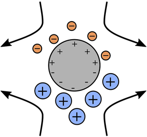
Induced-charge electro-osmosis (ICEO) refers to the fluid flow around a polarizable surface (e.g. a metal) in an electrolyte solution under an external electric field (Squires & Bazant Reference Squires and Bazant2010). The basic mechanism in ICEO is that the applied field induces an inhomogeneous distribution of polarization charges on the surface, resulting in the formation of a volumetric distribution of ionic charge density adjacent to it. The ions in this ‘Debye layer’ screen the polarization charge, such that the fluid elements at a distance of several Debye lengths from the surface are essentially uncharged, or electro-neutral. In most practical situations the Debye length is much smaller than the characteristic length scale of the surface, a scenario known as the ‘thin-Debye-layer’ limit. The applied field exerts an electric stress on (charged) fluid elements in the Debye layer, the component of which tangent to the local surface is compensated by a hydrodynamic stress to maintain mechanical equilibrium; thus, a (electro-osmotic) fluid flow occurs. This flow appears as a ‘slip velocity’ boundary condition at the length scale of the particle, which animates flow throughout the electroneutral ‘bulk’ electrolyte. Since the external field induces the Debye layer and then promotes the electric stress within it, the flow is nonlinear in the applied field strength, scaling as the square of the field strength for sufficiently weak fields. Importantly, this means that time-averaged, or rectified, flows can be driven by alternating (ac) external fields, which is attractive for pumping and mixing in microfluidic devices (Squires & Bazant Reference Squires and Bazant2004a). ICEO is related to ac electro-osmosis (ACEO), in which flows are also generated around polarizable surfaces, the prototypical scenario there being a pair of co-planar electrodes addressed by an ac voltage (Ramos et al. Reference Ramos, Morgan, Green and Castellanos1999). In ACEO flow is animated atop the driving electrodes, whereas in ICEO flow can be driven around an electrically isolated object, such as a metal post.
Interest in ICEO in the West was sparked just over 15 years ago by the work of Squires & Bazant (Reference Squires and Bazant2004a,Reference Squires and Bazantb). Those authors noted, however, that similar flows had previously been studied, theoretically and experimentally, in the Russian literature (Gamayunov, Murtsovkin & Dukhin Reference Gamayunov, Murtsovkin and Dukhin1986; Gamayunov, Mantrov & Murtsovkin Reference Gamayunov, Mantrov and Murtsovkin1992). Squires & Bazant (Reference Squires and Bazant2004b) analysed in detail the ICEO flow around an infinitely long, ideally polarizable circular cylinder in a binary, symmetric electrolyte. Here, ‘ideally polarizable’ means that the cylinder cannot support electrochemical reactions at its surface; consequently, no current flows through it. The time-averaged ICEO flow is quadrupolar and directed from the ‘polar’ axis of the cylinder that is parallel to the applied field to the ‘equatorial’ axis that is perpendicular to the field. Experiments by Levitan et al. (Reference Levitan, Devasenathipathy, Studer, Ben, Thorsen, Squires and Bazant2005) confirmed this flow pattern around a platinum wire in a KCl solution. An oppositely directed (equator-to-pole) flow was observed around a spherical tin particle in distilled water by Gamayunov et al. (Reference Gamayunov, Mantrov and Murtsovkin1992), which they attributed to current flow across the particle surface; i.e. that particle was not ideally polarizable. Squires & Bazant (Reference Squires and Bazant2006) predicted that ‘breaking symmetries’ in ICEO – via inhomogeneous shape or surface properties – implies net pumping of fluid past fixed objects or motion of freely suspended particles. The former effect has been harnessed to fabricate ICEO ‘micropumps’ (Paustian et al. Reference Paustian, Pascall, Wilson and Squires2014). The latter effect is termed induced-charge electrophoresis (ICEP) and was observed in experiments by Gangwal et al. (Reference Gangwal, Cayre, Bazant and Velev2008) on (partially) gold-coated spheres of polystyrene latex in NaCl under ac fields.
In this article, we consider another ‘broken symmetry’ in ICEO; the symmetry of the cations and anions in the electrolyte. Almost all theoretical works on ICEO have assumed a binary, symmetric electrolyte, where the cations and anions have equal magnitude of valences and equal diffusion coefficients. An exception is the recent work by Hashemi Amrei, Miller & Ristenpart (Reference Hashemi Amrei, Miller and Ristenpart2020), of which more will be said later. Here, we analyse ICEO in binary electrolytes with cations and anions of equal valence but unequal diffusion coefficients, focusing on the prototypical case of a circular cylinder in the weak-field and thin-Debye-layer limits. All electrolytes have unequal ionic diffusion coefficients to some extent: perhaps the closest commonplace example of a symmetric electrolyte is KCl, for which the ratio of anion to cation diffusion coefficients, which we shall denote by  $\gamma$, equals
  $1.038$ (Vanýsek Reference Vanýsek and Haynes2012). Feng et al. (Reference Feng, Huang, Wong and Duan2018) observed ICEO around a gold-coated stainless steel cylinder in an ac field: in the weak-field regime at a frequency of
  $1.5$ kHz and electrolyte concentration of 1 mM, the measured flow velocity in an NaCl (
 $\gamma =1.523$) solution was around twice as strong as in NaDS (sodium dodecyl sulphate,
  $\gamma =0.479$), and approximately four times as much as in measurements on KCl by Canpolat, Qian & Beskok (Reference Canpolat, Qian and Beskok2013). Further, it has been shown that an asymmetry in ion diffusion coefficients is a necessary ingredient, along with Faradaic reactions and the presence of a Stern layer at the electrode surface, to predict flow reversals in ACEO over electrode arrays addressed by a travelling-wave voltage (García-Sánchez et al. Reference García-Sánchez, Ramos, González, Green and Morgan2009; González et al. Reference González, Ramos, García-Sánchez and Castellanos2010). This provides further motivation for the present study. We will find that an inequality in ionic diffusion coefficients fundamentally changes the ‘standard model’ of ICEO outlined by Squires & Bazant (Reference Squires and Bazant2004b): chiefly, for
  $\gamma \neq 1$, gradients in ion concentration, or concentration polarization, arises in the bulk electrolyte in the form of diffusive travelling waves. Whilst this concentration polarization has zero time average, it alters the rectified electro-osmotic slip velocity at the cylinder surface and drives rectified body forces in the bulk fluid, thereby affecting the time-averaged flow around the cylinder. A similar effect of concentration polarization was recently analysed by García-Sánchez, Loucaides & Ramos (Reference García-Sánchez, Loucaides and Ramos2017) for ACEO; specifically, see their equation (36). A key finding of our study, then, is that for any real electrolyte one cannot predict the rectified ICEO flow by only considering the flow due to electro-osmotic slip.
In § 2 the equations governing ICEO in an electrolyte with unequal diffusion coefficients are formulated and then specialized to the weak-field and thin-Debye-layer limits. In § 3 the system is solved and our results are compared against experimental studies. A conclusion is offered in § 4.
2. Problem formulation
An infinitely long circular cylinder of cross-sectional radius  $a^*$ is immersed in an unbounded binary electrolyte solution containing fully dissociated ions. Above, and henceforth, dimensional variables will be decorated with an asterisk superscript. The cations have valence
  $+\mathcal {Z}$ and diffusion coefficient
  $D^*_+$, and the anions have valence
  $-\mathcal {Z}$ and diffusion coefficient
  $D^*_-$. The cylinder is an ideally polarizable conductor that is initially uncharged. A spatially uniform, alternating electric field
  $\boldsymbol {E}^*\cos (\omega ^*t^*)$ is applied normal to the axis of cylinder. Here,
  $t^*$ denotes time;
  $\omega ^*$ is angular frequency; and
  $\boldsymbol {E}^*$ is a constant vector whose magnitude,
  $E^*$, specifies the field strength. The applied field induces polarization charges on the surface of the cylinder, which, in turn, are enveloped by a Debye layer of ions. The spatial extent of this layer is characterized (for dilute electrolytes) by the Debye length
 \begin{equation} \kappa^{*-1}=\sqrt{\frac{\epsilon^*k^*T^*}{2\mathcal{Z}^2e^{*2}n^{*}}}, \end{equation}
where  $\epsilon ^*$ is the solution permittivity;
  $k^*$ is Boltzmann's constant;
  $T^*$ is the absolute temperature;
  $e^{*}$ is charge on a proton; and
  $n^{*}$ is the equilibrium number concentration of cations and anions. We adopt the standard electrokinetic equations for dilute electrolytes (Saville Reference Saville1977). The ion concentrations satisfy the conservation law
 \begin{equation} \frac{\partial n^*_{\pm}}{\partial t^*}+\nabla^{*}\boldsymbol{\cdot}\boldsymbol{j}^*_{\pm}=0, \end{equation}
where  $n^*_{\pm }$ is the ion concentration, with the plus sign taken for cations, and the minus sign for anions. The ionic flux density
 \begin{equation} \boldsymbol{j}^*_{\pm}=\mp\frac{D^*_{\pm}\mathcal{Z}e^*}{k^*T^*}n^*_{\pm} \nabla^*\phi^*-D^*_{\pm}\nabla^*n^*_{\pm}+\boldsymbol{u}^*n^*_{\pm}, \end{equation}
which is a combination of electro-migration in a gradient of electric potential  $\phi ^*$ (the first term); diffusion (the second term); and advection with the fluid velocity
  $\boldsymbol {u}^*$. The potential satisfies the Poisson equation
 \begin{equation} -\epsilon^*\nabla^{*2}\phi^*=\mathcal{Z}e^*(n^*_+-n^*_-). \end{equation}
The fluid flow is governed by the Stokes equations,
 \begin{equation} \mu^*\nabla^{*2}\boldsymbol{u}^*-\boldsymbol{\nabla}^*p^*+\epsilon^*(\nabla^{*2}\phi^*)\nabla^*\phi^*=0 \quad \textrm{and}\quad \boldsymbol{\nabla}^{*}\boldsymbol{\cdot}\boldsymbol{u}^*=0, \end{equation}
where  $p^*$ is the dynamic pressure and
  $\mu ^*$ is the viscosity. In (2.5a,b), the first equation is a momentum balance on an inertialess fluid element accounting for an electric (Coulomb) body force, and the second equation stipulates that the fluid is incompressible.
We introduce polar coordinates  $(r^*,\theta ,z^*)$, where
  $r^*$ is the distance from the axis of the cylinder;
  $z^*$ is the distance along the axis; and
  $\theta$ is the angle from the direction of the applied field, measured anti-clockwise. Thus, far from the cylinder
 \begin{align} \boldsymbol{u}^*\to 0,\quad p^*\to 0,\quad n^*_{\pm}\to n^*\quad \textrm{and}\quad \phi^*\to -E^*r^*\cos\theta\cos(\omega^*t^*)\quad \textrm{as}\ r^*\to\infty. \end{align}
The first condition states that the velocity disturbance due to the (freely suspended) cylinder decays at large distances. We are at liberty to assert that the pressure approaches zero since it is defined up to an additive constant for an incompressible fluid. The remaining conditions state that the ion concentrations approach their equilibrium value and the electric field approaches the applied field. At the surface of the cylinder,  $r^*=a^*$, we impose
 \begin{equation} \boldsymbol{u}^*= 0,\quad \phi^*=0\quad \textrm{and}\quad \boldsymbol{e}_r\boldsymbol{\cdot}\boldsymbol{j}^*_{\pm}=0, \end{equation}
where  $\boldsymbol {e}_r$ is the unit normal vector along the
  $r^*$ direction. The first condition in (2.7a–c) imposes no slip and no fluid penetration at the cylinder surface. The second condition represents continuity of potential, where the conducting cylinder is an equipotential surface whose potential is chosen as zero. The third condition asserts an ideally polarizable surface that cannot admit an ionic flux. Finally, Gauss's law requires
  $q^*=-\epsilon ^*\boldsymbol {e}_{r}\boldsymbol {\cdot }\boldsymbol {\nabla }^*\phi ^*$ at
  $r^*=1$, where
  $q^*$ is the surface charge density. As noted by Schnitzer & Yariv (Reference Schnitzer and Yariv2012), Gauss's law does not represent an additional boundary condition; rather, it enables calculation of
  $q^*$ from knowledge of
  $\phi ^*$. Since the cylinder has no net charge the integral of
  $q^*$ over its cross-section is zero at all times.
The problem is now made dimensionless. We normalize distance with  $a^*$; time by
  $1/\omega ^*$; ion concentration by
  $n^*$; and electrical potential by the ‘thermal voltage’
  $\phi _T^*=k^*T^*/\mathcal {Z}e^*$, which is approximately
  $26\ \textrm {mV}$ at
  $T^*=298\ \textrm {K}$ for a univalent electrolyte. Balancing electric and viscous stresses in (2.5a,b) yields the velocity and pressure scales
  $\epsilon ^*\phi _T^{*2}/\mu ^*a^*$ and
  $\epsilon ^*\phi _T^{*2}/a^{*2}$, respectively. Therefore, the conservation laws (2.2) along with ionic fluxes (2.3) give the dimensionless equations
 \begin{equation} \frac{a^{*2}\omega^{*}}{D^*_{\pm}}\frac{\partial n_{\pm}}{\partial t}\mp\boldsymbol{\nabla}\boldsymbol{\cdot}(n_{\pm}\boldsymbol{\nabla}\phi)-\nabla^2n_{\pm}+m_{\pm} \boldsymbol{u}\boldsymbol{\cdot}\boldsymbol{\nabla} n_{\pm}=0. \end{equation}
Note, to derive (2.8) we have used the continuity condition. In (2.8), and henceforth, the lack of an asterisk superscript on a variable indicates that it is the dimensionless counterpart of the appropriate dimensional variable: for instance, the dimensionless time  $t=\omega ^*t^*$. The quantities
  $m_{\pm }=\epsilon ^*\phi _T^{*2}/\mu ^*D^*_{\pm }$ are dimensionless ionic drag coefficients with a value of around 0.5 for univalent aqueous electrolytes at room temperature (Dukhin Reference Dukhin1993; Schnitzer & Yariv Reference Schnitzer and Yariv2012). The dimensionless version of Poisson's equation reads
 \begin{equation} \delta^2\nabla^2\phi=-\tfrac{1}{2}(n_+-n_-), \end{equation}
in which  $\delta =1/(\kappa ^*a^*)$ is the (small) ratio of the Debye length to cylinder radius. The dimensionless Stokes equations are
 \begin{equation} \nabla^2\boldsymbol{u}-\boldsymbol{\nabla} p+(\nabla^2\phi)\boldsymbol{\nabla}\phi=0\quad \textrm{and}\quad \boldsymbol{\nabla}\boldsymbol{\cdot}\boldsymbol{u}=0. \end{equation}
At large distances the dimensionless boundary conditions read
 \begin{equation} \boldsymbol{u}\to 0,\quad p\to 0,\quad n_{\pm}\to 1\quad \textrm{and}\quad \phi\to -\beta r\cos\theta\cos t\quad \textrm{as}\ r\to\infty, \end{equation}
where  $\beta =E^*a^*/\phi _T^*$ is the ratio of the applied voltage across the cylinder relative to the thermal voltage. Using (2.3), the dimensionless boundary conditions at the surface of the cylinder are
 \begin{equation} \boldsymbol{u}=0,\quad \phi=0\quad \textrm{and}\quad \boldsymbol{e}_r\boldsymbol{\cdot}(\mp n_{\pm}\boldsymbol{\nabla}\phi-\boldsymbol{\nabla} n_{\pm})=0\quad \textrm{at}\ r=1. \end{equation}
The dimensionless version of Gauss's law is  $q=-\delta \boldsymbol {e}_r\boldsymbol {\cdot }\boldsymbol {\nabla }\phi$ at
  $r=1$, where the surface charge density has been normalized with
  $\epsilon ^*\kappa ^*\phi _T^*$.
The dimensionless groups  $a^{*2}\omega ^*/D^*_{\pm }$ naturally emerge from the normalization process: these are ratios of the ion diffusion times over the cross-sectional radius,
  $a^{*2}/D^*_{\pm }$, to the time scale on which the field oscillates,
  $1/\omega ^*$. We define
  $\gamma =D_-^*/D_+^*$ as the ratio of the anion to cation diffusion coefficients and
  $\alpha =a^{*2}\omega ^*/D^*_-$. Hence,
  $a^{*2}\omega ^*/D^*_+=\gamma \alpha$. Thus, the Debye-layer charging under the alternating field and, consequently, the time-averaged ICEO flow, are governed by four dimensionless groups:
  $\alpha$,
  $\beta$,
  $\gamma$ and
  $\delta$.
It is useful to work with the dimensionless mean ‘salt’ concentration  $c={\frac {1}{2}}(n_++n_-)$ and dimensionless mean charge density
  $\rho ={\frac {1}{2}}(n_+-n_-)$. From (2.8) these quantities satisfy
 \begin{align} &\frac{\alpha(\gamma+1)}{2}\frac{\partial c}{\partial t}+\frac{\alpha(\gamma-1)}{2}\frac{\partial\rho}{\partial t}-\boldsymbol{\nabla}\boldsymbol{\cdot}(\rho\boldsymbol{\nabla}\phi)-\nabla^2c+\frac{m_++m_-}{2}\boldsymbol{u} \boldsymbol{\cdot}\boldsymbol{\nabla} c\nonumber\\ &\quad +\frac{m_+-m_-}{2}\boldsymbol{u}\boldsymbol{\cdot}\boldsymbol{\nabla}\rho=0, \end{align}
 \begin{align} &\frac{\alpha(\gamma+1)}{2}\frac{\partial \rho}{\partial t}+\frac{\alpha(\gamma-1)}{2} \frac{\partial c}{\partial t}-\boldsymbol{\nabla}\boldsymbol{\cdot}(c\boldsymbol{\nabla}\phi)-\nabla^2 \rho+\frac{m_++m_-}{2}\boldsymbol{u}\boldsymbol{\cdot}\boldsymbol{\nabla} \rho\nonumber\\ &\quad +\frac{m_+-m_-}{2}\boldsymbol{u}\boldsymbol{\cdot}\boldsymbol{\nabla} c=0. \end{align}
In the far field we require from (2.11)
 \begin{equation} c\to 1\quad \textrm{and}\quad \rho\to 0\quad \textrm{as}\ r\to\infty, \end{equation}
and at the surface of the cylinder from (2.12) we have
 \begin{equation} \boldsymbol{e}_r\boldsymbol{\cdot}(\rho\boldsymbol{\nabla}\phi+\boldsymbol{\nabla} c)=0 \quad \textrm{and}\quad \boldsymbol{e}_r\boldsymbol{\cdot} (c\boldsymbol{\nabla}\phi+\boldsymbol{\nabla} \rho)=0\quad \textrm{at}\ r=1. \end{equation}
Additionally, we define the dimensionless salt flux  $\boldsymbol {j}=\boldsymbol {j}_++\boldsymbol {j}_-$, where
  $\boldsymbol {j}_+$ and
  $\boldsymbol {j}_-$ are the dimensionless flux of cations and anions normalized on
  $n^*D_+/a^*$. It is readily shown from (2.8) that
 \begin{equation} \boldsymbol{j}=(\gamma-1)c\boldsymbol{\nabla}\phi-(\gamma+1)\rho\boldsymbol{\nabla}\phi-(\gamma+1)\boldsymbol{\nabla} c+(\gamma-1)\boldsymbol{\nabla}\rho+2m_+\boldsymbol{u}c. \end{equation}
Similarly, let  $\boldsymbol {i}=\boldsymbol {j}_+-\boldsymbol {j}_-$ denote the dimensionless current density, normalized by
  $\mathcal {Z}e^*D_+^*n^*/a^*$. From (2.8) we have
 \begin{equation} \boldsymbol{i}=-(\gamma+1)c\boldsymbol{\nabla}\phi+(\gamma-1)\rho\boldsymbol{\nabla}\phi+(\gamma-1)\boldsymbol{\nabla} c-(\gamma+1)\boldsymbol{\nabla}\rho+2m_+\boldsymbol{u}\rho. \end{equation}
The discussion in this section has furnished a mathematical model for ICEO around a cylinder for a binary electrolyte with unequal ionic diffusivities. The governing equations are coupled and nonlinear; a numerical solution must be sought in general. Moving forward we make assumptions to enable analytical progress; importantly, these assumptions are experimentally relevant.
2.1. Thin-Debye-layer limit
Experiments are typically conducted with micron-scale posts or particles in electrolytes at milli-molar concentration, for which the thin-Debye-layer limit,  $\delta \ll 1$, is pertinent. In this situation, the electrolyte can be conceptually partitioned into two regions: (i) a bulk region corresponding to
  $r=O(1)$; and a thin Debye layer with
  $r-1=O(\delta )$. From (2.9), the charge density
  $\rho$ in the bulk electrolyte is zero to leading-order in
  $\delta$; the bulk is electroneutral. Thus, from (2.13a) and (2.13b) the leading-order bulk ion transport equations are
 \begin{gather} \frac{\alpha(\gamma+1)}{2}\frac{\partial c}{\partial t}+\frac{m_++m_-}{2}\boldsymbol{u} \boldsymbol{\cdot}\boldsymbol{\nabla} c=\nabla^2c, \end{gather}
 \begin{gather}\frac{\alpha(\gamma-1)}{2}\frac{\partial c}{\partial t}+\frac{m_+-m_-}{2} \boldsymbol{u}\boldsymbol{\cdot}\boldsymbol{\nabla} c=\boldsymbol{\nabla}\boldsymbol{\cdot}(c\boldsymbol{\nabla}\phi) . \end{gather}
The bulk salt flux and current are from (2.16) and (2.17), respectively,
 \begin{gather} \boldsymbol{j}=(\gamma-1)c\boldsymbol{\nabla}\phi-(\gamma+1)\boldsymbol{\nabla} c+2m_+\boldsymbol{u}c, \end{gather}
 \begin{gather}\boldsymbol{i}=-(\gamma+1)c\boldsymbol{\nabla}\phi+(\gamma-1)\boldsymbol{\nabla} c. \end{gather}
Evidently, in an electroneutral electrolyte with unequal ionic diffusion coefficients: (i) a gradient in salt concentration drives bulk current; and (ii) an electric field drives a bulk salt flux. This does not happen in a symmetric electrolyte.
The ion transport within the Debye layer can be analysed by defining an inner radial coordinate  $R=(r-1)/\delta$ with
  $R=O(1)$ as
  $\delta \to 0$. Introducing this rescaling into (2.13a) and (2.13b), it is readily shown that the ion concentrations vary in
  $R$, at leading order, according to a quasi-equilibrium Boltzmann distribution provided that
  $\delta ^2\alpha \ll 1$. The restriction that
  $\delta ^2\alpha \ll 1$ suffices for anions and cations since
  $\gamma$ is typically
  $O(1)$ for aqueous electrolytes. Since
  $\delta ^2\alpha =\omega ^*/D_-^*\kappa ^{*2}$, this means that the Debye layer charges quasi-steadily provided that the time period for variations in the field (
 $1/\omega ^*$) is much smaller than the Debye relaxation time (
 $1/D_-^*\kappa ^{*2}$). Again, this is indeed the case for ICEO experiments. The variation of ion concentrations, electric potential, and fluid flow in a quasi-equilibrium Debye layer have been analysed thoroughly in several works: see e.g. Khair & Squires (Reference Khair and Squires2008), Olesen, Bazant & Bruus (Reference Olesen, Bazant and Bruus2010) and Schnitzer & Yariv (Reference Schnitzer and Yariv2012). Thus, we need not repeat such a discussion here. However, to proceed we recall that the effect of the flow in the Debye layer on the bulk velocity field can be represented as a ‘slip velocity’ boundary condition. Let
  $\boldsymbol {u}=u\boldsymbol {e}_r+v\boldsymbol {e}_{\theta }$ denote the fluid velocity vector in cylindrical coordinates, where
  $\boldsymbol {e}_{\theta }$ is a unit vector in the
  $\theta$ direction. For ICEO the dimensionless slip velocity is (Schnitzer & Yariv Reference Schnitzer and Yariv2012)
 \begin{equation} u=0\quad \textrm{and}\quad v=-\phi\frac{\partial\phi}{\partial\theta}+2\ln\left[1-\tanh^2\left( \frac{\phi}{4}\right)\right]\frac{\partial\ln c}{\partial\theta}\quad \textrm{at}\ r=1. \end{equation}
In (2.20) the location  $r=1$ should be interpreted as at the outer edge of the Debye layer, which is, of course, indistinguishable from the actual surface of the cylinder on lengths
  $r=O(1)$. Further,
  $-\phi$ represents the (spatially non-uniform) dimensionless zeta potential; hence, the first term in
  $v$ is identified as electro-osmosis and the second as diffusio-osmosis. Additionally, the Debye-layer analysis employed in the above-mentioned works yields effective boundary conditions on the bulk salt and potential fields, to be applied at
  $r=1$. A discussion of these conditions is postponed until after the limit of a weak applied field is invoked, which is done next.
2.2. Weak-field expansion
The bulk ion transport and flow equations are now considered in the weak-field regime,  $\beta \ll 1$. The limit
  $\beta \to 0$ is regular, as opposed to the singular limit
  $\delta \to 0$; hence, there is no issue with taking the former limit after the latter. We pose the expansions
  $c=1+\beta c_1$,
  $\phi =\beta \phi _1$,
  $\boldsymbol {u}=\beta ^2\boldsymbol {u}_1$ and
  $p=\beta ^2p_1$, where the quadratic leading-order scaling of velocity and pressure is obtained from the electro-osmotic contribution to the slip velocity (2.20). Therefore, the linearized ion transport equations become from (2.18a) and (2.18b)
 \begin{gather} \frac{\partial c_1}{\partial t}=\frac{2}{\alpha(1+\gamma)}\nabla^2c_1, \end{gather}
 \begin{gather}\nabla^2\phi_1=\frac{\alpha(\gamma-1)}{2}\frac{\partial c_1}{\partial t}. \end{gather}
From (2.10a,b), the leading-order bulk flow satisfies
 \begin{equation} \nabla^2\boldsymbol{u}_1-\boldsymbol{\nabla} p_1+\frac{\alpha(\gamma-1)}{2}\frac{\partial c_1}{\partial t}\boldsymbol{\nabla}\phi_1=0\quad \textrm{and}\quad \boldsymbol{\nabla}\boldsymbol{\cdot}\boldsymbol{u}_1=0, \end{equation}
where we have used (2.21b) in rewriting the Coulomb body force. The linearized equations are subject to
 \begin{equation} \boldsymbol{u}_1\to 0,\quad p_1\to 0,\quad c_1\to 0\quad \textrm{and}\quad \phi_1\to -r\cos\theta\cos t\quad \textrm{as}\ r\to\infty. \end{equation}
Using (2.20), the fluid velocity satisfies the slip condition
 \begin{equation} u_1=0\quad \textrm{and}\quad v_1=-\phi_1\frac{\partial\phi_1}{\partial\theta}\quad \textrm{at}\ r=1. \end{equation}
Evidently, the leading-order, i.e.  $O(\beta ^2)$, slip is solely due to electro-osmosis; a diffusio-osmotic contribution arises first at
  $O(\beta ^3)$.
To complete the linearized bulk equations we need boundary conditions for (2.21a) and (2.21b) at  $r=1$. This requires an analysis of ion accumulation within the Debye layer, driven by transport from (or to) the bulk and transport along the layer. The latter effect, known as ‘surface conduction’, is negligible for ICEO provided
  $\delta \textrm {e}^{\beta }\ll 1$ (Schnitzer & Yariv Reference Schnitzer and Yariv2012); this inequality is obviously satisfied in the weak-field limit. Further, to first order in
  $\beta$ the Debye layer behaves as a linear capacitor, i.e. with a capacitance that is independent of the (local) zeta potential, for which the (local) dimensional surface charge density
  $q^*=-\epsilon ^*\kappa ^*\phi _T^*\beta \phi _1$ (Squires & Bazant Reference Squires and Bazant2004b). The time variation of
  $q^*$ arises due to the current supplied by the bulk electrolyte; hence, we have from charge conservation
  $\partial q^*/\partial t^*=\boldsymbol {i}^*\boldsymbol {\cdot }\boldsymbol {e}_r$, where
  $\boldsymbol {i}^*$ is the dimensional bulk current density. From (2.19b),
 \begin{equation} \boldsymbol{i}^*=\frac{\mathcal{Z}e^*D_+^*n^*}{a^*}([(\gamma-1)\boldsymbol{\nabla} c_1-(\gamma+1)\boldsymbol{\nabla}\phi_1]\beta+O(\beta^2)). \end{equation}
Hence, the linearized, dimensionless charge conservation condition yields
 \begin{equation} 2\gamma\alpha\delta\frac{\partial\phi_1}{\partial t}=(\gamma+1)\frac{\partial\phi_1}{\partial r}-(\gamma-1)\frac{\partial c_1}{\partial r}\quad \textrm{at}\ r=1. \end{equation}
A second consequence of the Debye layer acting as a linear capacitor is that it does not uptake a net amount of ‘salt’ from the bulk. Said differently, at every station in  $\theta$ the Debye layer expels as many co-ions as it takes up counter-ions. Therefore, the linearized mean salt flux
  $\boldsymbol {j}$ must vanish at
  $r=1$. Now, from (2.19a) we have
 \begin{equation} \boldsymbol{j}=\left[(\gamma-1)\boldsymbol{\nabla}\phi_1-(\gamma+1)\boldsymbol{\nabla} c_1\right]\beta +O(\beta^2), \end{equation}
and requiring  $\boldsymbol {j}$ to vanish at
  $O(\beta )$ yields the boundary condition
 \begin{equation} \frac{\partial c_1}{\partial r}=\frac{\gamma-1}{\gamma+1}\frac{\partial \phi_1}{\partial r}\quad \textrm{at}\ r=1. \end{equation}
In summary, (2.21a), (2.21b) and (2.22a,b), along with boundary conditions (2.23), (2.24), (2.26) and (2.28), govern the weak-field ICEO around a cylinder in an electrolyte with unequal ionic diffusivities. The fact that  $\gamma \neq 1$ has two important consequences. First, the bulk ion concentration is non-uniform in an alternating field, or any unsteady field for that matter. This transient ‘concentration polarization’ occurs to ensure there is no net salt uptake in the Debye layer during its charging. Second, the concentration polarization results in a body force density in the bulk fluid; consequently, the bulk flow around the cylinder is not solely animated by electro-osmotic slip (as it would be for a symmetric electrolyte).
The factor  $\alpha \delta =(a^*/D_-^*\kappa ^*)/(1/\omega ^*)$ appearing in (2.26) represents the ratio of an ‘
 $RC$’ time,
  $a^*/D_-^*\kappa ^*$, to the time period of the alternating field. It is over this
  $RC$ scale that the Debye layer charges. Consequently, the concentration polarization varies on the
  $RC$ time also, as opposed to the much longer bulk diffusion time
  $a^{*2}/D_-^*$. Indeed, for slow oscillations
  $\omega ^*\sim 1/(a^{*2}/D_-^*)$ we have
  $\alpha \delta \sim \delta$, implying that the left-hand side of (2.26) is negligibly small. On dropping this term, the resulting system of equations admits a solution with a uniform salt concentration,
  $c_1=0$. Hence, there is negligible concentration polarization under sufficiently slow oscillations and, therefore, zero concentration polarization in a steady (direct current) field. Finally, our assumption of quasi-steady Stokes flow (2.5a,b) requires that the momentum diffusion time
  $a^{*2}/\nu ^*$, where
  $\nu ^*$ is the kinematic viscosity of the fluid, is much smaller than the
  $RC$ time. This can be invalidated in experiments on ICEO in ac fields (Canpolat et al. Reference Canpolat, Qian and Beskok2013); hence, a proper description of the time-dependent flow would require the unsteady Stokes equations. However, our focus is on the rectified flow for which (2.5a,b) suffices, since the time average of a periodic, unsteady Stokes flow solves the quasi-steady Stokes equations under the time-averaged body force density.
3. Results and comparison to experiments
The system of equations developed in the preceding section is now solved. We first demonstrate that our analysis recovers the standard picture of ICEO in a symmetric electrolyte (Squires & Bazant Reference Squires and Bazant2004b), before moving to asymmetric electrolytes. Our interest is in describing the long-time ion transport and fluid flow under ac forcing; we do not consider how this state is attained upon initiation of the field.
3.1. Symmetric electrolyte,  $\gamma =1$

For a symmetric electrolyte (2.28) reduces to  $\partial c_1/\partial r=0$ at
  $r=1$. Thus, the trivial solution
  $c_1=0$ is obtained; the salt concentration is not perturbed from its equilibrium value. Physically, for a symmetric electrolyte the applied field does not generate a bulk salt flux, since the ions have equal mobilities; consequently, a compensating salt gradient is not required to ensure that the Debye layer has no net salt uptake. Since
  $c_1=0$, the potential
  $\phi _1$ is a harmonic function. Prompted by the far-field boundary condition on
  $\phi _1$ (2.23), we seek a solution of the form
 \begin{equation} \phi_1=\left[-r\cos t+\frac{1}{r}\textrm{Re}(\mathcal{D}\textrm{e}^{\textrm{i} t})\right]\cos\theta, \end{equation}
where Re denotes the real part, and  $\textrm {i}=\sqrt {-1}$. The applied field represents an oscillating dipole ‘at infinity,’ and the disturbance due to the cylinder is a dipole at the origin. Application of (2.26) yields the dipole strength
 \begin{equation} \mathcal{D}=\frac{\alpha\delta\textrm{i}-1}{\alpha\delta\textrm{i}+1}. \end{equation}
Hence, from (2.24) the slip velocity is
 \begin{equation} v_1=2\sin(2\theta)\left[\textrm{Re}\left(\frac{\textrm{e}^{\textrm{i} t}}{1+\alpha\delta\textrm{i}}\right)\right]^2\quad \textrm{at}\ r=1, \end{equation}
which consists of frequency-doubled (relative to the ac forcing) and rectified components. The latter is readily found as
 \begin{equation} \langle v_1\rangle = \frac{\sin (2\theta)}{1+(\alpha\delta)^2}\quad \textrm{at}\ r=1, \end{equation}
where  $\langle \cdots \rangle$ denotes a time average over one period of the field oscillation. The magnitude of the slip velocity decreases with increasing frequency due to the insufficient time for the Debye layer to charge up during the time period of the field oscillation. The rectified slip velocity animates a steady bulk flow that is conveniently represented by a streamfunction
  $\langle \psi \rangle$, which is related to the velocity field components via
 \begin{equation} \langle u_1\rangle=\frac{1}{r}\frac{\partial\langle\psi\rangle}{\partial\theta}\quad \textrm{and}\quad \langle v_1\rangle=-\frac{\partial\langle\psi\rangle}{\partial r}. \end{equation}
The streamfunction satisfies the biharmonic equation  $\nabla ^4\langle \psi \rangle =0$. A straightforward calculation using (3.4) yields
 \begin{equation} \langle\psi\rangle=\frac{1}{2[1+(\alpha\delta)^2]}\left(\frac{1}{r^2}-1\right)\sin (2\theta). \end{equation}
Equation (3.6) describes a quadrupolar flow, where the fluid velocity is directed toward the cylinder along the polar axis ( $\theta =0$) and away from the cylinder along the equatorial axis (
 $\theta ={\rm \pi} /2$). At large distances, the flow appears as a (two-dimensional) stresslet, with a radial velocity decaying like
  $\langle u_1\rangle \sim 1/r$. We reiterate that the results in this subsection were derived by Squires & Bazant (Reference Squires and Bazant2004b); the purpose of this presentation is to serve as a contrast to the case of an asymmetric electrolyte, discussed next.
3.2. Asymmetric electrolyte, $\gamma \neq 1$

The linearized salt perturbation satisfies the diffusion equation (2.21a), to which a solution  $c_1=\textrm {Re}[\,f(r) \, \textrm {e}^{\textrm {i} t}]\cos \theta$ is sought, corresponding to a dipolar salt distribution. Substituting this ansatz into (2.21a) yields
 \begin{equation} \frac{\textrm{d}^2f}{\textrm{d}r^2}+\frac{1}{r}\frac{\textrm{d}f}{\textrm{d}r}- \left[\frac{1}{r^2}+m^2\right]f=0, \end{equation}
where  $m=\sqrt {\alpha (1+\gamma )\textrm {i}/2}$. The solutions of this equation are the first-order modified Bessel functions
  $I_1(mr)$ and
  $K_1(mr)$. The function
  $I_1(mr)$ diverges exponentially at large
  $r$ and is thus discarded, whereas
  $K_1(mr)$ decays exponentially. Thus, we have
 \begin{equation} c_1=\textrm{Re}[\mathcal{A}K_1(mr)\,\textrm{e}^{\textrm{i} t}]\cos\theta, \end{equation}
where  $\mathcal {A}$ is a complex-valued constant. At distances
  $|m|r\gg 1$ (3.8) has the asymptotic form
 \begin{equation} c_{1} \sim\textrm{Re}\left[\frac{\mathcal{A}}{m^{1/2}}\textrm{e}^{\textrm{i}(t-r/\mathcal{L})}\right] \textrm{e}^{-r/\mathcal{L}}\left(\frac{\rm \pi}{2r^{1/2}}\right)\cos\theta, \end{equation}
which describes damped travelling waves of concentration polarization that propagate from the cylinder with wavelength and attenuation distance  $\mathcal {L}=\sqrt {4/[\alpha (1+\gamma )]}$. The amplitude factor
  $r^{-1/2}$ arises due to the curvature of the cylinder. The equivalent dimensional length scale is
  $\mathcal {L}^*=a^*\mathcal {L}=(2D^*_a/\omega ^*)^{1/2}$, where
  $D_a^*=2D_+^*D_-^*/(D_+^*+D_-^*)$ is the ambipolar diffusion coefficient of the electrolyte. The frequency scaling
  $\mathcal {L}^*\sim \omega ^{*-1/2}$ has been identified in several studies of Debye layers under ac forcing (Shilov & Dukhin Reference Shilov and Dukhin1970; Chew & Sen Reference Chew and Sen1982; DeLacey & White Reference DeLacey and White1982; González et al. Reference González, Ramos, García-Sánchez and Castellanos2010; García-Sánchez et al. Reference García-Sánchez, Loucaides and Ramos2017; Hashemi Amrei et al. Reference Hashemi Amrei, Bukosky, Rader, Ristenpart and Miller2018). For oscillations at the ‘ambipolar
  $RC$’ frequency,
  $\omega ^*=O(\kappa ^*D^*_a/a^*)$, we have
  $\mathcal {L}^*/a^*=O(\delta ^{1/2})$; this is a distinguished limit in which the concentration polarization is confined to a ‘diffusion layer’ atop the Debye layer. The one-dimensional transport between planar, parallel electrodes under strong ac forcing at such frequencies was analysed by Olesen et al. (Reference Olesen, Bazant and Bruus2010) for a symmetric electrolyte.
The potential is written as  $\phi _1=\phi _1^H+\phi _1^P$, where the harmonic homogenous solution,
  $\phi _1^H$, is again (3.1), although now the value of the dipole strength
  $\mathcal {D}$ is different, by virtue of the salt perturbation. Hence, even though there is no diffusio-osmotic contribution to the slip velocity, the salt field still influences the slip through its effect on
  $\mathcal {D}$, which, in turn, affects the electro-osmotic slip. The particular solution satisfies from (2.21b)
 \begin{equation} \nabla^2\phi_1^P=\frac{\alpha(\gamma-1)}{2}\textrm{Re}[\textrm{i} \mathcal{A}K_1(mr)\,\textrm{e}^{\textrm{i} t}]\cos\theta. \end{equation}
Hence, we pose  $\phi _1^P=\textstyle {\frac {1}{2}}\alpha (\gamma -1)\textrm {Re}[\textrm {i}\mathcal {A}g(r) \, \textrm {e}^{\textrm {i} t}]\cos \theta$. Substituting this ansatz into (3.10) yields
 \begin{equation} \frac{\textrm{d}^2g}{\textrm{d}r^2}+\frac{1}{r}\frac{\textrm{d}g}{\textrm{d}r}- \frac{g}{r^2}=K_1(mr). \end{equation}
The solution to this equation is found by variation of parameters as  $g=K_1(mr)/m^2$. Therefore, the potential is
 \begin{equation} \phi_1=\left[-r\cos t+\frac{1}{r}\textrm{Re}(\mathcal{D}\textrm{e}^{\textrm{i} t})+\frac{\gamma-1}{\gamma+1}\textrm{Re}[\mathcal{A}K_1(mr)\,\textrm{e}^{\textrm{i} t}]\right]\cos\theta. \end{equation}
The constants  $\mathcal {A}$ and
  $\mathcal {D}$ are found from the boundary conditions (2.26) and (2.28). Some straightforward, but tedious, working returns
 \begin{equation} \mathcal{D}=\frac{\textrm{i}\alpha\delta(1-\mathcal{Q})-\dfrac{\gamma+1}{2\gamma}}{ \textrm{i}\alpha\delta(1+\mathcal{Q})+\dfrac{\gamma+1}{2\gamma}}, \end{equation}
where
 \begin{equation} \mathcal{Q}=\frac{(\gamma-1)^2}{2\gamma}\frac{K_1(m)}{m[K_0(m)+K_2(m)]}, \end{equation}
and  $K_0(m)$ and
  $K_2(m)$ are zeroth- and second-order modified Bessel functions. Notice that
  $\mathcal {D}$ reduces to (3.2) for
  $\gamma =1$. The real and imaginary parts of
  $\mathcal {D}$ are plotted in figure 1 versus the rescaled frequency
  $\delta \alpha _{{a}}$ for KCl (
 $\delta =1.038$), NaOH (
 $\delta =3.953$) and HCl (
 $\delta =0.218$). The values of
  $\delta$ are obtained from measurements of ionic diffusion coefficients at infinite dilution (Vanýsek Reference Vanýsek and Haynes2012). Here
  $\alpha _a=\omega ^{*2}a^{*2}/D^*_a=(1+\gamma )\alpha /2$ is the oscillation frequency normalized on the ambipolar diffusion coefficient. This is the most appropriate dimensionless frequency to use, since the value of
  $\mathcal {D}$ at fixed
  $\alpha _a$ does not change under the transformation
  $\gamma \to 1/\gamma$; that is, it does not matter if the cations are more mobile than the anions, or vice versa, as long as the ratio of the mobilities is constant. At high frequency (
 $\delta \alpha _{{a}}\gg 1$) the double layer does not have time to charge and the bulk field lines look like those around a conducting cylinder, for which
  $\textrm {Re}(\mathcal {D})=1$. In contrast, at low frequency the double layer almost completely charges; hence, the bulk field does not penetrate the Debye layer and the field lines resemble those around an insulating cylinder, for which
  $\textrm {Re}(\mathcal {D})=-1$. The imaginary part of
  $\mathcal {D}$ decays at both extremes of frequency, like
  $1/(\delta \alpha _{a})^2$, where the Debye-layer charging is essentially in phase with the applied field. The maximal out-of-phase response is at
  $\delta \alpha _{{a}}=O(1)$. The influence of a difference in diffusion coefficients is noticeable: for instance, at
  $\delta \alpha _{{a}}=1$ the sign of
  $\textrm {Re}(\mathcal {D})$ is positive for KCl but negative for NaOH and HCl. Finally, the constant
  $\mathcal {A}$ is then
 \begin{equation} \mathcal{A}=\frac{(\gamma+1)(\gamma-1)}{2\gamma}\frac{1+\mathcal{D}}{m[K_0(m)+K_2(m)]}. \end{equation}
Having determined the linearized potential and salt concentration, we now turn to the resulting fluid flow. The rectified streamfunction is split as  $\langle \psi \rangle =\langle \psi ^H\rangle +\langle \psi ^P\rangle$ Here, from (2.22a,b), the ‘homogenous streamfunction’ satisfies the unforced Stokes equations with the slip condition (2.24), whereas the ‘particular streamfunction’ satisfies the Stokes equations with a body force density arising from transient concentration polarization, and a zero velocity boundary condition at
  $r=1$. We consider
  $\langle \psi _H\rangle$ first. To that end, using (3.12), the slip velocity is
 \begin{equation} v_1^H=\tfrac{1}{2}\sin(2\theta)\left[\textrm{Re}(\varPhi_0\,\textrm{e}^{\textrm{i} t})\right]^2\quad \textrm{at}\ r=1, \end{equation}
in which
 \begin{equation} \varPhi_0=-\frac{\dfrac{\gamma+1}{\gamma}}{\textrm{i}\alpha\delta(1+\mathcal{Q})+\dfrac{\gamma+1}{2\gamma}}. \end{equation}
The rectified slip velocity
 \begin{equation} \langle v_1^H\rangle=\tfrac{1}{4}\left[(\textrm{Re}[\varPhi_0])^2+(\textrm{Im}[\varPhi_0])^2\right] \sin(2\theta)\quad \textrm{at}\ r=1, \end{equation}
where Im denotes the imaginary part. The variation of the magnitude of the slip velocity with frequency  $\delta \alpha _a$ for KCl, NaOH and HCl is shown in figure 2. The magnitude monotonically decreases with increasing
  $\delta \alpha _a$, due to a diminished tangential component of the field with increasing
  $\delta \alpha _a$, since field lines are instead drawn into the Debye layer to charge it. The decay in slip velocity is like
  $1/(\delta \alpha _a)^2$ at
  $\delta \alpha _a\gg 1$ for all three electrolytes. The slip animates a rectified flow represented by the streamfunction
 \begin{equation} \langle\psi^H\rangle=\frac{1}{8}\left[(\textrm{Re}[\varPhi_0])^2+(\textrm{Im}[\varPhi_0])^2\right] \left(\frac{1}{r^2}-1\right)\sin (2\theta). \end{equation}
Evidently, this flow is always directed from the pole to equator, regardless of the value of  $\gamma$.

Figure 1. (a) Real and (b) imaginary parts of the dipole strength  $\mathcal {D}$ for three electrolytes versus
  $\delta \alpha _a$. The number in parentheses gives the value of
  $\delta$ for each electrolyte.

Figure 2. Variation of the magnitude of the slip velocity versus rescaled frequency  $\delta \alpha _a$ for three electrolytes.
To determine  $\langle \psi _P\rangle$ we take the curl of (2.22a,b) to obtain
 \begin{equation} \nabla^2\boldsymbol{\omega}_1^P=-\frac{\alpha(\gamma-1)}{2}\frac{\partial\boldsymbol{\nabla} c_1}{\partial t}\wedge\boldsymbol{\nabla}\phi_1, \end{equation}
where  $\boldsymbol {\omega }_1^P=\boldsymbol {\nabla }\wedge \boldsymbol {u}_1^P$ is the vorticity of the velocity field,
  $\boldsymbol {u}_1^P$, generated by the body force density in (2.22a,b). This vorticity can also be written
  $\boldsymbol {\omega }_1^P=-\nabla ^2\psi ^P\boldsymbol {e}_z$, where
  $\psi ^P$ is the streamfunction associated with
  $\boldsymbol {u}_1^P$, whose time average equals
  $\langle \psi ^P\rangle$. Here,
  $\boldsymbol {e}_z$ is a unit vector along the axis of the cylinder. Therefore, from (3.20),
  $\psi ^P$ satisfies the forced biharmonic equation
 \begin{equation} \nabla^4\psi^P=\frac{\alpha(\gamma-1)}{2r}\left(\frac{\partial\phi_1}{\partial\theta}\frac{\partial^2c_1}{\partial t\partial r}-\frac{\partial\phi_1}{\partial r}\frac{\partial^2c_1}{\partial t\partial \theta}\right). \end{equation}
From (3.8) we define  $\partial ^2c_1/\partial \theta \partial t=\textrm {Re}[\varPhi _1(r) \, \textrm {e}^{\textrm {i} t}]\sin \theta$ and
  $\partial ^2c_1/\partial r\partial t=\textrm {Re}[\varPhi _2(r) \, \textrm {e}^{\textrm {i} t}]\cos \theta$, where
 \begin{equation} \varPhi_1=-\textrm{i} \mathcal{A}K_1(mr)\quad \textrm{and}\quad \varPhi_2=-\frac{m}{2}\textrm{i} \mathcal{A}[K_0(mr)+K_2(mr)]. \end{equation}
From (3.12) we define  $\partial \phi _1/\partial \theta =\textrm {Re}[\varPhi _3(r) \, \textrm {e}^{\textrm {i} t}]\sin \theta$ and
  $\partial \phi _1/\partial r=\textrm {Re}[\varPhi _4(r) \, \textrm {e}^{\textrm {i} t}]\cos \theta$, where
 \begin{equation} \varPhi_3=r-\frac{\mathcal{D}}{r}-\mathcal{A}\frac{\gamma-1}{\gamma+1}K_1(mr) \quad \textrm{and}\quad \varPhi_4=-1-\frac{\mathcal{D}}{r^2}-\frac{m}{2}\mathcal{A}\frac{\gamma-1}{\gamma+1}[K_0(mr)+K_2(mr)]. \end{equation}
Therefore, we have
 \begin{align} &\frac{\partial\phi_1}{\partial\theta}\frac{\partial^2c_1}{\partial t\partial r}-\frac{\partial\phi_1}{\partial r} \frac{\partial^2c_1}{\partial t\partial \theta}\nonumber\\ &\quad =\frac{\sin(2\theta)}{2}\left[\left(\textrm{Re}[\varPhi_3]\cos t- \textrm{Im}[\varPhi_3]\sin t\right)\left(\textrm{Re}[\varPhi_2]\cos t-\textrm{Im}[\varPhi_2] \sin t\right)\right]\nonumber\\ &\qquad -\left(\textrm{Re}[\varPhi_4]\cos t-\textrm{Im}[\varPhi_4]\sin t \right)\left(\textrm{Re}[\varPhi_1]\cos t-\textrm{Im}[\varPhi_1]\sin t\right), \end{align}
which is expanded out as
 \begin{align} \frac{\partial\phi_1}{\partial\theta}\frac{\partial^2c_1}{\partial t\partial r}-\frac{\partial\phi_1}{\partial r}\frac{\partial^2c_1}{\partial t\partial \theta}& =\frac{\sin(2\theta)}{4}\left(\textrm{Re}[\varPhi_3]\textrm{Re}[\varPhi_2]+ \textrm{Im}[\varPhi_3]\textrm{Im}[\varPhi_2]\right.\nonumber\\ &\quad\left. -\textrm{Re}[\varPhi_4]\textrm{Re}[\varPhi_1]- \textrm{Im}[\varPhi_4]\textrm{Im}[\varPhi_1]\right)+\cdots, \end{align}
where  $\cdots$ indicates terms that average to zero over an oscillation cycle. Therefore, using (3.25) in (3.21) yields
 \begin{align} \nabla^4\langle\psi^P\rangle& =\frac{\alpha(\gamma-1)}{8r}\left[ \textrm{Re}(\varPhi_3)\textrm{Re}(\varPhi_2)+\textrm{Im}(\varPhi_3)\textrm{Im} (\varPhi_2)-\textrm{Re}(\varPhi_4)\textrm{Re}(\varPhi_1)\right.\nonumber\\ &\quad \left.-\textrm{Im}(\varPhi_4) \textrm{Im}(\varPhi_1)\right]\sin(2\theta). \end{align}
To proceed we let  $\langle \psi ^P\rangle ={\frac {1}{8}}\alpha (\gamma -1)Q(r)\sin (2\theta )$, and from (3.26) the function
  $Q(r)$ satisfies
 \begin{align} \frac{\textrm{d}^4Q}{\textrm{d}r^4}&+\frac{2}{r}\frac{\textrm{d}^3Q}{\textrm{d}r^3}- \frac{9}{r^2}\frac{\textrm{d}^2Q}{\textrm{d}r^2}+\frac{9}{r^3}\frac{\textrm{d}Q}{\textrm{d}r}=\frac{1}{r}[\textrm{Re}(\varPhi_3)\textrm{Re}(\varPhi_2)\nonumber\\ &+\textrm{Im}(\varPhi_3) \textrm{Im}(\varPhi_2)-\textrm{Re}(\varPhi_4)\textrm{Re}(\varPhi_1)-\textrm{Im}(\varPhi_4) \textrm{Im}(\varPhi_1)], \end{align}
subject to
 \begin{equation} Q=0,\quad \frac{\textrm{d}Q}{\textrm{d}r}=0\quad \textrm{at}\ r=1,\quad \textrm{and} \quad \frac{Q}{r}\to 0,\quad \frac{\textrm{d}Q}{\textrm{d}r}\to0\quad \textrm{as}\ r\to\infty. \end{equation}
The boundary conditions at  $r=1$ specify zero fluid velocity at the surface of the cylinder, and the conditions as
  $r\to \infty$ specify attenuation of the velocity at large distances. The appropriate homogenous solutions to (3.27) are
  $1/r^2$ and
  $r^0$. Thus, we write
  $Q(r)=c_1+c_2/r^2+Q^P(r)$, where
  $c_1$ and
  $c_2$ are constants, and
  $Q^P(r)$ is the particular solution to (3.27). Equation (3.27) is then solved numerically by integrating back from a distance
  $r_{{out}}$ to
  $r=1$ and choosing
  $c_1$ and
  $c_2$ to enforce the boundary conditions there. The value of
  $r_{{out}}$ is chosen to be a distance of several
  $\mathcal {L}$ from
  $r=1$. This gives
  $c_2={\frac {1}{2}}({\textrm {d}Q^P}/{\textrm {d}r})|_{r=1}$ and
  $c_1=-c_2-Q^P|_{r=1}$, where the values of
  $Q^P|_{r=1}$ and
  ${\textrm {d}Q^P}/{\textrm {d}r}|_{r=1}$ are determined from the numerical integration.
The forcing in (3.27) is exponentially small at  $|m|r\gg 1$; hence, the far-field flow is dominated by the homogenous solution and asymptotes to the stresslet field
 \begin{equation} \langle \boldsymbol{u}^P_1\rangle = \frac{c_1\alpha(\gamma-1)}{4}\frac{\cos(2\theta)}{r}\boldsymbol{e}_r+O(r^{-3}) \quad \textrm{as}\ r\to\infty. \end{equation}
Likewise, the far-field flow due to the slip velocity is readily calculated from (3.19). Thus, the total far-field flow takes the form  $\langle \boldsymbol {u}_1\rangle \sim \mathcal {S}\cos (2\theta )/r$, where the stresslet strength
 \begin{equation} \mathcal{S}=\tfrac{1}{4}\left(c_1\alpha(\gamma-1)-\left[(\textrm{Re}[\varPhi_0])^2+(\textrm{Im}[\varPhi_ 0])^2\right]\right) \end{equation}
provides a convenient measure of the flow magnitude and direction. A flow directed from the pole to equator requires  $\mathcal {S}<0$. This is not evident from (3.30), as the sign of
  $c_1$ is unknown a priori; however, it is observed that
  $\mathcal {S}<0$ from our numerical calculations (figure 3). That is, we do not find that unequal ionic diffusion coefficients alone lead to large-scale flow reversal, i.e. equator-to-pole flow. This is consistent with analysis of ACEO in the weak-field regime, for which flow reversal requires Faradaic reactions and a Stern layer at the electrodes in addition to unequal diffusion coefficients (González et al. Reference González, Ramos, García-Sánchez and Castellanos2010).

Figure 3. Variation of the stresslet strength  $\mathcal {S}$ versus rescaled frequency
  $\delta \alpha _a$ for three electrolytes.
3.3. Comparison to experiments
Feng et al. (Reference Feng, Huang, Wong and Duan2018) measured the ICEO flow around a gold-coated stainless steel cylinder with a cross-sectional radius of  $a=175\ \mathrm {\mu } \textrm {m}$. Figure 5 in their paper reports the maximum flow velocity along the polar axis of the cylinder as a function of field strength in NaCl (
 $\gamma =1.523$), NaDS (
 $\gamma =0.479$), KCl (
 $\gamma =1.038$) and
  $\textrm {CaCl}_2$ at a frequency of 1.5 kHz and electrolyte concentration of 1 mM. Note,
  $\textrm {CaCl}_2$ is an electrolyte with unequal cationic and anionic valences and therefore outside the scope of the present work. The flow velocity is observed to increase with the square of the field strength, as predicted in the weak-field limit. Under these conditions,
  $\delta =5.6\times 10^{-5}$ and
  $\alpha =1.42\times 10^5$ for NaCl and
  $\alpha =4.51\times 10^5$ for NaDS; hence,
  $\delta \alpha _a=10.0$ for NaCl and
  $\delta \alpha _a=18.7$ for NaDS. The inset to their figure 5 shows that the ratio of maximum flow velocity to the field strength squared in NaCl is approximately
  $9\times 10^3\ \mathrm {\mu } \textrm {m} \ \textrm {s}^{-1}/\textrm {V}^{2} \ \textrm {cm}^{-2}$ and approximately
  $4.5\times 10^3 \ \mathrm {\mu } \textrm {m} \ \textrm {s}^{-1}/\textrm {V}^2 \ \textrm {cm}^{-2}$ in NaDS. That is, the maximum flow speed is approximately twice as much in NaCl as compared to NaDS. In comparison, our theory predicts a stresslet coefficient of
  $\mathcal {S}=-0.011$ for NaCl and
  $\mathcal {S}=-0.004$ for NaDS; suggesting the far-field flow in NaCl is approximately 2.8 times larger than in NaDS. The ratio of maximum flow velocity to the field strength squared in KCl is reported as approximately
  $2.5\times 10^3\ \mathrm {\mu } \textrm {m} \ \textrm {s}^{-1}/\textrm {V}^2 \ \textrm {cm}^{-2}$. This value is taken from experiments by Canpolat et al. (Reference Canpolat, Qian and Beskok2013) who measured ICEO around a gold-coated stainless steel cylinder of
  $a=335\ \mathrm {\mu } \textrm {m}$ (see figure 6 in that paper). Thus, for KCl we have
  $\delta =2.9\times 10^{-5}$,
  $\alpha =5.20\times 10^5$ and
  $\delta \alpha _a=15.4$, for which we predict
  $\mathcal {S}=-0.004$, i.e. the same value as in NaDS, whereas the experiments suggest a slower flow in KCl than in NaDS. As noted by Feng et al. (Reference Feng, Huang, Wong and Duan2018), however, their measurements were conducted in a microfluidic device with different dimensions to that of Canpolat et al. (Reference Canpolat, Qian and Beskok2013), which could contribute to the discrepancy with our theory, which, additionally, assumes an unbounded electrolyte. In summary, we view our predictions as being in fair agreement with these measurements.
4. Conclusion
We considered ICEO around a cylinder subject to an ac electric field in a binary electrolyte with unequal ionic diffusion coefficients. Our analysis was conducted in the limits of a weak applied field and thin Debye layer. The inequality of the diffusion coefficients results in concentration polarization waves in the bulk electrolyte, which alter the time-averaged fluid flow around the cylinder. The appropriate time scale on which the Debye layer charges, and hence the flow develops, was identified as the ambipolar  $RC$ time
  $a^*/\kappa ^*D_a^*$. The ambipolar diffusivity
  $D_a^*$ is weighted toward the ion with the lower diffusion coefficient; hence, it is the slow ion that is the rate-limiting species for Debye-layer charging, as expected. The ‘standard model’ of ICEO in the weak-field and thin-Debye-layer limits assumes an ohmic bulk electrolyte with no concentration gradients, wherein the potential is a harmonic function, and the fluid flow is solely animated by electro-osmotic slip (Squires & Bazant Reference Squires and Bazant2004b). These assumptions do not hold for an electrolyte with unequal diffusion coefficients: concentration polarization results in a non-ohmic bulk in which Coulomb body forces contribute to the time-averaged flow. The standard model is valid under a steady field, since the concentration polarization we predict is transient. However, note that most experiments use ac fields and, of course, all experiments use electrolytes with unequal diffusion coefficients. Therefore, it may prove useful to summarize our findings in terms of an ‘extended standard model’ for ICEO, valid for an arbitrary (fixed) geometry in the weak field and thin-Debye-layer limits. To that end, recall that
  $\phi =\beta \phi _1$ and
  $c=1+\beta c_1$ are the dimensionless potential and salt concentration to first order in field strength
  $\beta$. From (2.21a) and (2.21b) these quantities satisfy
 \begin{equation} \alpha_a\frac{\partial c_1}{\partial t}=\nabla^2c_1\quad \textrm{and}\quad \nabla^2\phi_1=\alpha_a\frac{\gamma-1}{\gamma+1}\frac{\partial c_1}{\partial t}, \end{equation}
where, recall,  $\alpha _a=\omega ^*a^{*2}/D_a^*$. The leading-order velocity and pressure,
  $\boldsymbol {u}=\beta ^2\boldsymbol {u}_1$ and
  $p=\beta ^2p_1$, respectively, satisfy, from (2.22a,b),
 \begin{equation} \nabla^2\boldsymbol{u}_1-\boldsymbol{\nabla} p_1+\alpha_a\frac{\gamma-1}{\gamma+1}\frac{\partial c_1}{\partial t}\boldsymbol{\nabla}\phi_1=0\quad \textrm{and}\quad \boldsymbol{\nabla}\boldsymbol{\cdot}\boldsymbol{u}_1=0. \end{equation}
At large distances  $c_1$,
  $\boldsymbol {u}_1$, and
  $p_1$ all vanish, while
  $\phi _1$ approaches the imposed field. Let
  $\boldsymbol {n}$ denote the outward unit normal vector to the surface. Then the Debye-layer charging and zero salt flux conditions, (2.26) and (2.28), respectively, generalize to
 \begin{gather} \frac{4\gamma\alpha_a\delta}{1+\gamma}\frac{\partial\phi_1}{\partial t}= (\gamma+1)\boldsymbol{n}\boldsymbol{\cdot}\boldsymbol{\nabla}\phi_1-(\gamma-1) \boldsymbol{n}\boldsymbol{\cdot}\boldsymbol{\nabla} c_1, \end{gather}
 \begin{gather}\boldsymbol{n}\boldsymbol{\cdot}\boldsymbol{\nabla} c_1= \frac{\gamma-1}{\gamma+1}\boldsymbol{n}\boldsymbol{\cdot} \boldsymbol{\nabla} \phi_1. \end{gather}
Finally, the fluid velocity is subject to the electro-osmotic slip condition  $\boldsymbol {u}=-\phi _1\boldsymbol {\nabla }_s\phi _1$, where
  $\boldsymbol {\nabla }_s=(\boldsymbol {I}-\boldsymbol {n}\boldsymbol {n})\boldsymbol {\cdot }\boldsymbol {\nabla }$ is the surface gradient operator, in which
  $\boldsymbol {I}$ is the identity tensor.
Recently, Hashemi Amrei et al. (Reference Hashemi Amrei, Miller and Ristenpart2020) analysed how unequal ionic diffusivities (and valences) affect ICEO around a charged, conducting cylinder. They considered a scenario where the (electrically isolated and hence fixed charge) cylinder is located between two planar, parallel electrodes subject to an oscillatory potential difference. The cylinder is assumed small enough that the ion transport between the electrodes is not affected by its presence. As predicted in earlier numerical work from this group (Hashemi Amrei et al. Reference Hashemi Amrei, Bukosky, Rader, Ristenpart and Miller2018), an inequality in the ionic diffusion coefficients results in a steady component to the electric potential in the electrolyte, which persists to a distance from each electrode that varies with the inverse square root of the field frequency (cf. our discussion of the diffusion layer in § 2). This was termed as an ‘asymmetric rectified electric field’ or ‘AREF’ for short. The magnitude of the AREF affects the time-averaged flow around the cylinder; notably, a flow reversal is seen under the transformation  $\gamma \to 1/\gamma$. Hashemi Amrei et al. (Reference Hashemi Amrei, Miller and Ristenpart2020) used the standard model for ICEO, thereby neglecting concentration polarization, which we have shown is inexorable in an electrolyte with unequal diffusion coefficients. It would be interesting to see how concentration polarization affects the ICEO flow due to an AREF.
Finally, our work points to other interesting questions: for instance, how does a difference in diffusion coefficients affect ICEP or ‘dipolophoresis’ (i.e. the combination of ICEP and dielectrophoresis) in ac fields? What about multicomponent electrolytes with unequal valences, or other time varying fields (e.g. a suddenly applied field)? It would also be interesting to relax the weak-field constraint. Experiments by Peng et al. (Reference Peng, Lazo, Shiyanovskii and Lavrentovich2014) have observed a time-averaged concentration polarization in ICEO flow around an immobilized metal cylinder. Our calculations predict zero time-averaged concentration polarization; thus, we expect that those observations are due to processes (e.g. surface conduction) that are operative at larger field strengths. However, as noted by Schnitzer & Yariv (Reference Schnitzer and Yariv2012), going beyond the weak-field limit would entail a complicated mathematical analysis, arising in part from the now nonlinear capacitance of the Debye layer. For instance, this implies that the concentration polarization occurs at multiple frequency overtones of the ac forcing, where the amplitude of each overtone is a nonlinear function of field strength.
Acknowledgements
We acknowledge support from the National Science Foundation through grant no. CBET-2002120.
Declaration of interests
The authors report no conflict of interest.


