3.1. Kirchhoff–Helmholtz integral

For this, we adapt the approach used for the Laplace and Helmholtz equations; see, for example, Lighthill (Reference Lighthill1986, § 8.1), Jackson (Reference Jackson1999, § 1.8), Martin (Reference Martin2006, § 5.6) and Pierce (Reference Pierce2019, § 4.6). For two arbitrary functions $f$ and $g$ we write

(3.1)\begin{equation} f(N^2\nabla_{{h}}^2-\omega^2\nabla^2)g-g(N^2\nabla_{{h}}^2-\omega^2\nabla^2)f = \boldsymbol{\nabla}\boldsymbol{\cdot}[f(N^2\boldsymbol{\nabla}_{{h}}-\omega^2\boldsymbol{\nabla})g-g(N^2\boldsymbol{\nabla}_{{h}}-\omega^2\boldsymbol{\nabla})f], \end{equation}

which upon integration inside a volume $V$ delimited by the surface $S$ of outward normal $\boldsymbol {n}$, and application of the divergence theorem, gives

(3.2)\begin{align} & \int_V [f(N^2\nabla_{{h}}^2-\omega^2\nabla^2)g - g(N^2\nabla_{{h}}^2-\omega^2\nabla^2)f] \,\mathrm{d}^3x \nonumber\\ &\quad = \int_S \left[ f \left( N^2\frac{\partial}{\partial n_{{h}}}- \omega^2\frac{\partial}{\partial n} \right) g - g \left(N^2\frac{\partial}{\partial n_{{h}}}- \omega^2\frac{\partial}{\partial n} \right) f \right] \mathrm{d}^2S, \end{align}

where $\partial /\partial n = \boldsymbol {n}\boldsymbol {\cdot }\boldsymbol {\nabla }$ and $\partial /\partial n_{{h}} = \boldsymbol {n}\boldsymbol {\cdot }\boldsymbol {\nabla }_{{h}}$.

We apply this Green's theorem to the volume $V_+$ exterior to the oscillating body, delimited internally by the surface $S$ of the body (with outward normal $-\boldsymbol {n}$) and externally by a surface $S_\infty$ at infinity, as shown in figure 1. The volume interior to the body is denoted as $V_-$. We choose a fixed observation point $\boldsymbol {x}$ in either $V_+$ or $V_-$, and denote the variable integration point in $V_+$ as $\boldsymbol {x}'$. We take for $f$ the internal potential $\psi (\boldsymbol {x}')$ at $\boldsymbol {x}'$, and for $g$ the propagator $G(\boldsymbol {x}-\boldsymbol {x}')$ from $\boldsymbol {x}'$ to $\boldsymbol {x}$. Here, $G$ is the Green's function of the wave equation, corresponding to unit point forcing and satisfying

(3.3)\begin{equation} (N^2\nabla_{{h}}^2-\omega^2\nabla^2)G(\boldsymbol{x}) = \delta(\boldsymbol{x}), \end{equation}

with $\delta$ the Dirac delta function, together with the causality condition that $G$ be analytic in the upper half of the complex $\omega$-plane. We assume that both $G$ and $\psi$ decay fast enough at infinity for the contribution of $S_\infty$ to vanish, and will come back to this assumption later in § 8. We obtain the Kirchhoff–Helmholtz integral

(3.4a)\begin{align} & \int_S \left[G(\boldsymbol{x}-\boldsymbol{x}')\left(N^2\frac{\partial}{\partial n'_{{h}}}- \omega^2\frac{\partial}{\partial n'}\right)\psi(\boldsymbol{x}')-\psi(\boldsymbol{x}') \left(N^2\frac{\partial}{\partial n'_{{h}}}- \omega^2\frac{\partial}{\partial n'}\right) G(\boldsymbol{x}-\boldsymbol{x}')\right]\mathrm{d}^2S' \nonumber\\ &\quad = \psi(\boldsymbol{x})\quad (\boldsymbol{x} \in V_+), \end{align}

(3.4b)\begin{align} &\quad = 0\quad (\boldsymbol{x} \in V_-), \end{align}

where $\partial /\partial n' = \boldsymbol {n}'\boldsymbol {\cdot }\boldsymbol {\nabla }'$ and $\partial /\partial n'_{{h}} = \boldsymbol {n}'\boldsymbol {\cdot }\boldsymbol {\nabla }'_{{h}}$, with $\boldsymbol {n}' = \boldsymbol {n}(\boldsymbol {x}')$.

Figure 1. Surfaces for the derivation of the Kirchhoff–Helmholtz integral.

Letting now $\boldsymbol {x}$ approach $S$ from within $V_+$, we obtain

(3.5)\begin{equation} \varPsi(\boldsymbol{x})+\int_S\varPsi(\boldsymbol{x}')\left(N^2\frac{\partial}{\partial n'_{{h}}}- \omega^2\frac{\partial}{\partial n'}\right)G(\boldsymbol{x}-\boldsymbol{x}')\,\mathrm{d}^2S' =\int_SU_n(\boldsymbol{x}')G(\boldsymbol{x}-\boldsymbol{x}')\,\mathrm{d}^2S', \end{equation}

an integral relation between the surface values $\varPsi$ of the internal potential (hence the pressure) and $U_n$ of the normal velocity, to be satisfied for all $\boldsymbol {x}$ on the outer side $S_+$ of $S$. Given the pressure this provides an integral equation of the first kind for the velocity, and given the velocity an equation of the second kind for the pressure. Once it is solved, the waves are expressed through the fluid, for $\boldsymbol {x} \in V_+$, as

(3.6)\begin{equation} \psi(\boldsymbol{x})=\int_S\left[U_n(\boldsymbol{x}')G(\boldsymbol{x}-\boldsymbol{x}')- \varPsi(\boldsymbol{x}')\left(N^2\frac{\partial}{\partial n'_{{h}}}- \omega^2\frac{\partial}{\partial n'}\right)G(\boldsymbol{x}-\boldsymbol{x}')\right]\mathrm{d}^2S'. \end{equation}

This expression combines two terms: a single-layer potential

(3.7)\begin{equation} \psi_{{s}}(\boldsymbol{x}) =\int_S \sigma(\boldsymbol{x}')G(\boldsymbol{x}-\boldsymbol{x}')\,\mathrm{d}^2S', \end{equation}

generated by the surface distribution of monopoles

(3.8)\begin{equation} q_{{s}}(\boldsymbol{x}) =\sigma(\boldsymbol{x})\delta_S(\boldsymbol{x}), \end{equation}

with density

(3.9)\begin{equation} \sigma(\boldsymbol{x}) = U_n(\boldsymbol{x}), \end{equation}

where $\delta _S$ is the Dirac delta function of support $S$, such that, if $S(\boldsymbol {x}) = 0$ is the equation of the surface, $\delta _S(\boldsymbol {x}) = |\boldsymbol {\nabla } S|\delta [S(\boldsymbol {x})]$; and a double-layer potential

(3.10)\begin{equation} \psi_{{d}}(\boldsymbol{x})=\int_S \mu(\boldsymbol{x}')\left(N^2\frac{\partial}{\partial n'_{{h}}}- \omega^2\frac{\partial}{\partial n'}\right)G(\boldsymbol{x}-\boldsymbol{x}')\,\mathrm{d}^2S', \end{equation}

generated by the surface distribution of dipoles

(3.11)\begin{equation} q_{{d}}(\boldsymbol{x})={-}\left(N^2\frac{\partial}{\partial n_{{h}}}- \omega^2\frac{\partial}{\partial n}\right)[\mu(\boldsymbol{x})\delta_S(\boldsymbol{x})], \end{equation}

with density

(3.12)\begin{equation} \mu(\boldsymbol{x}) ={-}\varPsi(\boldsymbol{x}). \end{equation}

See, for example, Jackson (Reference Jackson1999, § 1.6) for the introduction of such potentials in electrostatics, and Martin (Reference Martin2006, § 5.3) for non-dispersive waves.

The forcing is thus represented by the equivalent source

(3.13)\begin{equation} q(\boldsymbol{x}) =U_n(\boldsymbol{x})\delta_S(\boldsymbol{x})+\left(N^2\frac{\partial}{\partial n_{{h}}}- \omega^2\frac{\partial}{\partial n}\right)[\varPsi(\boldsymbol{x})\delta_S(\boldsymbol{x})]. \end{equation}

Such representation allows the extension of (3.6) to a viscous fluid, once the spectrum

(3.14)\begin{equation} q(\boldsymbol{k}) = \int q(\boldsymbol{x})\exp(-\mathrm{i}\boldsymbol{k}\boldsymbol{\cdot}\boldsymbol{x})\,\mathrm{d}^3x \end{equation}

is known, namely

(3.15)\begin{equation} q(\boldsymbol{k}) = \int_S[U_n(\boldsymbol{x})+ \mathrm{i}\boldsymbol{n}\boldsymbol{\cdot}(N^2\boldsymbol{k}_{{h}}-\omega^2\boldsymbol{k})\varPsi(\boldsymbol{x})] \exp(-\mathrm{i}\boldsymbol{k}\boldsymbol{\cdot}\boldsymbol{x})\,\mathrm{d}^2S, \end{equation}

with $\boldsymbol {k}$ the wave vector and $\boldsymbol {k}_{{h}}$ its horizontal projection. The extension follows the lines laid by Lighthill (Reference Lighthill1978, § 4.10), Hurley & Keady (Reference Hurley and Keady1997) and Voisin (Reference Voisin2020); it will be discussed further in § 6.2.

3.2. Green's function

To determine the Green's function we use the technique introduced by Bryan (Reference Bryan1889) for inertial waves and Hurley (Reference Hurley1972) for internal waves. In the frequency range $\omega > N$ of evanescent waves, (3.3), rewritten as

(3.16)\begin{equation} \left[(\omega^2-N^2)\frac{\partial^2}{\partial x^2}+ (\omega^2-N^2)\frac{\partial^2}{\partial y^2}+ \omega^2\frac{\partial^2}{\partial z^2}\right] G(\boldsymbol{x}) ={-}\delta(\boldsymbol{x}), \end{equation}

is elliptic. Stretching the coordinates according to

(3.17a–c)\begin{equation} x_\star = \frac{\omega}{N}x,\quad y_\star = \frac{\omega}{N}y,\quad z_\star = \left(\frac{\omega^2}{N^2}-1\right)^{1/2}z \end{equation}

transforms it into a Poisson equation, of known Green's function (Bleistein Reference Bleistein1984, § 6.2). Causality allows the continuation of the solution to the frequency range $0 < \omega < N$ of propagating waves. Continuation is implemented via Reference LighthillLighthill's (Reference Lighthill1978, § 4.9) radiation condition, namely by adding to the frequency a small positive imaginary part $\epsilon$ which is later allowed to tend to $0$; in other words, by performing the replacement

(3.18)\begin{equation} \omega \to \omega+\mathrm{i}0 = \lim_{\epsilon \to 0_+}(\omega+\mathrm{i}\epsilon). \end{equation}

The Green's function is obtained in three dimensions as

(3.19)\begin{equation} G(\boldsymbol{x}) = \frac{1}{4{\rm \pi} N(\omega^2-N^2)^{1/2}|\boldsymbol{x}_\star|}, \end{equation}

that is in unstretched coordinates

(3.20)\begin{equation} G(\boldsymbol{x}) =\frac{1}{4{\rm \pi}(\omega^2-N^2)^{1/2}(\omega^2r^2-N^2z^2)^{1/2}}, \end{equation}

with associated velocity

(3.21)\begin{equation} \boldsymbol{u}_G(\boldsymbol{x}) = (N^2\boldsymbol{\nabla}_{{h}}-\omega^2\boldsymbol{\nabla})G = \frac{\omega^2(\omega^2-N^2)^{1/2}\boldsymbol{x}}{4{\rm \pi}(\omega^2r^2-N^2z^2)^{3/2}}. \end{equation}

Similarly, in two dimensions, when the waves are independent of the horizontal coordinate $y$, the Green's function is

(3.22)\begin{equation} G(\boldsymbol{x}) ={-}\frac{\ln|\boldsymbol{x}_\star|}{2{\rm \pi}\omega(\omega^2-N^2)^{1/2}}. \end{equation}

Knowing the Green's function we can now solve (3.5) for prototypal oscillating bodies, namely an elliptic cylinder in two dimensions and a spheroid in three dimensions, in the next two sections.

4.1. Solution for $\omega > N$ and $(a/b)^2+(N/\omega )^2 > 1$

For $(a/b)^2+(N/\omega )^2 > 1$, the stretched ellipse has its foci along the horizontal axis, at $(x_\star = \pm c, z_\star = 0)$, with

(4.3)\begin{equation} c = (a_\star^2-b_\star^2)^{1/2}= \left[\frac{\omega^2}{N^2}a^2+\left(1-\frac{\omega^2}{N^2}\right)b^2\right]^{1/2}. \end{equation}

We introduce elliptic coordinates $(\xi ,\eta$) defined by

(4.4a,b)\begin{equation} x_\star = c\cosh\xi\cos\eta,\quad z_\star = c\sinh\xi\sin\eta, \end{equation}

with $0 \leqslant \xi < \infty$ and $0 \leqslant \eta < 2{\rm \pi}$. This definition is inverted in terms of the distances to the foci,

(4.5)\begin{equation} r_\pm = [(x_\star\pm c)^2+z_\star^2]^{1/2} = c(\cosh\xi\pm\cos\eta), \end{equation}

as

(4.6a,b)\begin{equation} \cosh\xi = \frac{r_+ + r_-}{2c},\quad \cos\eta = \frac{r_+{-}r_-}{2c}; \end{equation}

see Happel & Brenner (Reference Happel and Brenner1983, Appendix A) or Landau & Lifshitz (Reference Landau and Lifshitz1984, § 4). The spatial derivatives become

(4.7a)$$\begin{gather} c\frac{\partial}{\partial x_\star}= \frac{1}{\sinh^2\xi+\sin^2\eta} \left(\sinh\xi\cos\eta\frac{\partial}{\partial\xi}- \cosh\xi\sin\eta\frac{\partial}{\partial\eta}\right), \end{gather}$$

(4.7b)$$\begin{gather}c\frac{\partial}{\partial z_\star}= \frac{1}{\sinh^2\xi+\sin^2\eta}\left(\cosh\xi\sin\eta\frac{\partial}{\partial\xi}+ \sinh\xi\cos\eta\frac{\partial}{\partial\eta} \right), \end{gather}$$

where $\sinh ^2\xi +\sin ^2\eta = \sinh (\xi +\mathrm {i}\eta )\sinh (\xi -\mathrm {i}\eta )$.

At the ellipse, $\xi = \xi _0$ with

(4.8a,b)\begin{equation} a_\star = c\cosh\xi_0,\quad b_\star = c\sinh\xi_0, \end{equation}

so that

(4.9)\begin{equation} \xi_0 = \operatorname{arctanh}\left(\frac{b_\star}{a_\star}\right) = \operatorname{arctanh}\left[\frac{b}{a}\left(1-\frac{N^2}{\omega^2}\right)^{1/2}\right]. \end{equation}

There, $\eta$ reduces to the eccentric angle for the original ellipse, such that

(4.10a,b)\begin{equation} x = a\cos\eta,\quad z = b\sin\eta; \end{equation}

see Sommerville (Reference Sommerville1933, § IV.10) or Milne-Thomson (Reference Milne-Thomson1968, § 6.32). The arc length element follows as

(4.11)\begin{equation} \mathrm{d}l = (a^2\sin^2\eta+b^2\cos^2\eta)^{1/2}\,\mathrm{d}\eta, \end{equation}

and the outward normal as

(4.12)\begin{equation} \boldsymbol{n} =\frac{b\boldsymbol{e}_x\cos\eta+a\boldsymbol{e}_z\sin\eta} {(a^2\sin^2\eta+b^2\cos^2\eta)^{1/2}}, \end{equation}

where $\boldsymbol {e}_x$ and $\boldsymbol {e}_z$ are unit vectors along the $x$- and $z$-axes, respectively. The boundary integral equation (3.5) becomes

(4.13)\begin{equation} 2{\rm \pi}\varPsi(\eta)+\int_0^{2{\rm \pi}} \left[\varPsi(\eta')\frac{\partial}{\partial\xi'}+ \frac{(a^2\sin^2\eta'+b^2\cos^2\eta')^{1/2}}{\omega(\omega^2-N^2)^{1/2}} U_n(\eta')\right]\ln|\boldsymbol{x}_\star{-}\boldsymbol{x}'_\star|\,\mathrm{d}\eta'= 0, \end{equation}

where $\xi = \xi _0+0 > \xi ' = \xi _0$.

To solve it, we adapt the procedure used by Gorodtsov & Teodorovich (Reference Gorodtsov and Teodorovich1982) for the potential flow around a circular cylinder. The normal velocity $U_n(\eta )$ is expanded in circular functions as

(4.14)\begin{equation} (a^2\sin^2\eta+b^2\cos^2\eta)^{1/2} U_n(\eta)= c\sum_{m=0}^\infty[U_m^{(\mathrm{c})}\cos(m\eta)+U_m^{(\mathrm{s})}\sin(m\eta)], \end{equation}

with

(4.15)\begin{equation} cU_m^{(\mathrm{c},\mathrm{s})} =\frac{\epsilon_m}{2{\rm \pi}} \int_0^{2{\rm \pi}}(a^2\sin^2\eta+b^2\cos^2\eta)^{1/2}U_n(\eta) (\cos,\sin)(m\eta)\,\mathrm{d}\eta, \end{equation}

and the surface potential $\varPsi (\eta )$ as

(4.16)\begin{equation} \varPsi(\eta)=\sum_{m=0}^\infty[\varPsi_m^{(\mathrm{c})}\cos(m\eta)+\varPsi_m^{(\mathrm{s})}\sin(m\eta)], \end{equation}

with

(4.17)\begin{equation} \varPsi_m^{(\mathrm{c},\mathrm{s})} =\frac{\epsilon_m}{2{\rm \pi}} \int_0^{2{\rm \pi}}\varPsi(\eta)(\cos,\sin)(m\eta)\,\mathrm{d}\eta. \end{equation}

Here, $\epsilon _m = 1$ for $m = 0$ and $2$ for $m \geqslant 1$ is the Neumann factor. The Green's function has been shown by Morse & Feshbach (Reference Morse and Feshbach1953, p. 1202) to admit of the expansion

(4.18)\begin{align} \ln|\boldsymbol{x}_\star{-}\boldsymbol{x}'_\star| &= \xi_> + \ln\left(\frac{c}{2}\right)-\sum_{m=1}^\infty \frac{2}{m}\exp({-}m\xi_>)[\cosh(m\xi_<)\cos(m\eta)\cos(m\eta') \nonumber\\ &\quad +\sinh(m\xi_<)\sin(m\eta)\sin(m\eta')], \end{align}

where $\xi _< = \min (\xi ,\xi ')$ and $\xi _> = \max (\xi ,\xi ')$. Use of these expansions turns (4.13) into a diagonal (infinite) linear system, of solution

(4.19a)$$\begin{gather} \varPsi_0^{(\mathrm{c})} ={-}\frac{c}{\omega(\omega^2-N^2)^{1/2}} \xi_0U_0^{(\mathrm{c})},\quad \varPsi_0^{(\mathrm{s})} = 0, \end{gather}$$

(4.19b)$$\begin{gather}\varPsi_m^{(\mathrm{c},\mathrm{s})} = \frac{c}{\omega(\omega^2-N^2)^{1/2}} \frac{U_m^{(\mathrm{c},\mathrm{s})}}{m}\quad (m \ne 0). \end{gather}$$

Evaluation of the convolution integral (3.6), followed by differentiation according to (2.4), yields

(4.20)\begin{equation} p = \mathrm{i}\rho_0c(\omega^2-N^2)^{1/2}\left\{U_0^{(\mathrm{c})}\xi-\frac{1}{2} \sum_\pm\sum_{m=1}^\infty[U_m^{(\mathrm{c})}\pm\mathrm{i}U_m^{(\mathrm{s})}] \frac{\exp[{-}m(\xi-\xi_0\pm\mathrm{i}\eta)]}{m}\right\} \end{equation}

for the pressure, and

(4.21)\begin{equation} \boldsymbol{u} = \frac{1}{2}\sum_\pm \frac{(\omega^2-N^2)^{1/2}\boldsymbol{e}_x\pm\mathrm{i}\omega\boldsymbol{e}_z} {N\sinh(\xi\pm\mathrm{i}\eta)}\sum_{m=0}^\infty [U_m^{(\mathrm{c})}\pm\mathrm{i}U_m^{(\mathrm{s})}] \exp[{-}m(\xi-\xi_0\pm\mathrm{i}\eta)] \end{equation}

for the velocity.

4.2. Solution for $\omega > N$ and $(a/b)^2+(N/\omega )^2 < 1$

These results are continued analytically to $(a/b)^2+(N/\omega )^2 < 1$ by applying (3.18). The stretched ellipse has its foci along the vertical axis, at $(x_\star = 0,z_\star = \pm c')$, with

(4.22)\begin{equation} c' = \mathrm{i}c = \left[\left(\frac{\omega^2}{N^2}-1\right)b^2-\frac{\omega^2}{N^2}a^2\right]^{1/2}. \end{equation}

This prompts the introduction of elliptic coordinates $(\xi ',\eta )$, defined by

(4.23a,b)\begin{equation} x_\star = c'\sinh\xi'\cos\eta,\quad z_\star = c'\cosh\xi'\sin\eta, \end{equation}

where $0 \leqslant \xi ' < \infty$ and $0 \leqslant \eta < 2{\rm \pi}$. Writing

(4.24a,b)\begin{equation} x_\star = c\cosh\left(\xi'+\mathrm{i}\frac{\rm \pi}{2}\right)\cos\eta,\quad z_\star = c\sinh\left(\xi'+\mathrm{i}\frac{\rm \pi}{2}\right)\sin\eta, \end{equation}

the solution of the problem is seen to follow immediately from that in § 4.1, by replacing $\xi$ by $\xi '+\mathrm {i}{\rm \pi} /2$ and $c$ by $-\mathrm {i}c'$ throughout.

4.3. Solution for $\omega < N$

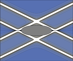
In the frequency range $0 < \omega < N$, the waves propagate at the angle $\theta _0 = \arccos (\omega /N)$ to the vertical. The semi-focal distance of the stretched ellipse becomes

(4.25)\begin{equation} c = (a^2\cos^2\theta_0+b^2\sin^2\theta_0)^{1/2}, \end{equation}

a quantity interpreted by Hurley (Reference Hurley1997) as the half-width of the wave beams delimited by the critical wave rays tangential to the ellipse on either side. The semi-axes become

(4.26a,b)\begin{equation} a_\star = a\cos\theta_0 = c\cos\eta_0,\quad b_\star = \mathrm{i}b\sin\theta_0 = \mathrm{i}c\sin\eta_0, \end{equation}

where

(4.27)\begin{equation} \eta_0 = \arctan\left(\frac{b}{a}\tan\theta_0\right) \end{equation}

is the eccentric angle of the critical points at which the critical rays are tangential to the ellipse. Both definitions are illustrated in figure 2.

Figure 2. Geometry for the beams of waves propagating (a) upward to the right and downward to the left, and (b) downward to the right and upward to the left.

The stretched elliptic coordinates $\xi$ and $\eta$ become complex, with $\xi$ taking the value $\xi _0 = \mathrm {i}\eta _0$ at the ellipse. The greatest difficulty here is the expression of $\xi$ and $\eta$ in more comprehensible coordinates. For a sphere or spheroid, Sarma & Krishna (Reference Sarma and Krishna1972) expressed the associated stretched spheroidal coordinates in terms of algebraic functions of the Cartesian coordinates, but did not consider the determination of these multivalued functions explicitly. Hendershott (Reference Hendershott1969) and Voisin (Reference Voisin1991) set the determination in the far field. Appleby & Crighton proceeded differently, for both the circular cylinder (Reference Appleby and Crighton1986) and the sphere (Reference Appleby and Crighton1987), decomposing the wave field into zones delimited by the critical rays, and investigating the properties of the stretched coordinates in each zone, concluding for the sphere that ‘this illustrates the difficulty of working in more comprehensible coordinates’. Davis (Reference Davis2012) combined the two approaches together for the sphere, expressing, in each zone, the stretched coordinates in terms of real algebraic functions of the Cartesian coordinates.

In actuality, Lighthill's radiation condition (3.18) allows both the stretched coordinates to be expressed in terms of the characteristic coordinates

(4.28a,b)\begin{equation} x_\pm = x\cos\theta_0\mp z\sin\theta_0,\quad z_\pm = \pm x\sin\theta_0+z\cos\theta_0, \end{equation}

shown in figure 2, and the associated multivalued functions to be determined unequivocally. The inversion formulae (4.5)–(4.6) are not convenient for this purpose. We proceed instead from (3.17), (4.3) and (4.4), writing

(4.29a,b)\begin{align} \cosh\xi\cos\eta = \frac{\omega x}{[\omega^2a^2+(N^2-\omega^2)b^2]^{1/2}},\quad \sinh\xi\sin\eta = \frac{(\omega^2-N^2)^{1/2}z}{[\omega^2a^2+(N^2-\omega^2)b^2]^{1/2}}. \end{align}

Expanding these for $\omega = N\cos \theta _0+\mathrm {i}\epsilon$, with $0 < \epsilon /N \ll 1$, we get

(4.30a,b)\begin{align} \cosh\xi\cos\eta \sim \frac{x}{c} \left(\cos\theta_0+\mathrm{i}\frac{\epsilon}{N}\frac{b^2}{c^2}\right),\quad \sinh\xi\sin\eta \sim \mathrm{i}\frac{z}{c} \left(\sin\theta_0-\mathrm{i}\frac{\epsilon}{N}\frac{a^2}{c^2}\cot\theta_0\right), \end{align}

so that

(4.31)\begin{equation} \cosh(\xi\pm\mathrm{i}\eta) \sim \frac{x_\pm}{c} \pm\mathrm{i}\frac{\epsilon}{N}\frac{\zeta_\pm}{c}\frac{d}{c\sin\theta_0}. \end{equation}

In addition to the quantities associated with the wave beams, namely their angle $\theta _0$ to the vertical, their half-width $c$ and the coordinates $(x_\pm ,z_\pm )$ perpendicular to and along them, respectively, this expression involves also quantities associated with the critical segments joining, for each beam, the opposite critical points on either side of the ellipse, namely their angle

(4.32)\begin{equation} \chi_0 = \arctan\left(\frac{b^2}{a^2}\tan\theta_0\right) \end{equation}

to the horizontal, their half-length

(4.33)\begin{equation} d = \frac{(a^4\cos^2\theta_0+b^4\sin^2\theta_0)^{1/2}}{c}, \end{equation}

and the coordinates

(4.34a,b)\begin{equation} \xi_\pm = x\cos\chi_{0} \mp z\sin\chi_0,\quad \zeta_\pm = \pm x\sin\chi_0+z\cos\chi_0 \end{equation}

along and perpendicular to them, respectively. These quantities, introduced by Voisin (Reference Voisin2020), are represented in figure 2.

We may then write

(4.35)\begin{equation} \xi\pm\mathrm{i}\eta = \operatorname{arccosh}\frac{x_\pm}{c} = \ln\left[\frac{x_\pm}{c}+\left(\frac{x_\pm^2}{c^2}-1\right)^{1/2}\right], \end{equation}

on the understanding that the determination of the square roots is set by the replacement

(4.36)\begin{equation} x_\pm \to x_\pm\pm \mathrm{i}0\operatorname{sign}\zeta_\pm, \end{equation}

so that, in particular,

(4.37a)\begin{align} (x_\pm^2-c^2)^{1/2} &= |x_\pm^2-c^2|^{1/2}\operatorname{sign} x_\pm \quad (|x_\pm| > c), \end{align}

(4.37b)\begin{align} &=\pm \mathrm{i} |x_\pm^2-c^2|^{1/2}\operatorname{sign}\zeta_\pm \quad (|x_\pm| < c). \end{align}

This determination, shown in figure 3, coincides with those in figures 3–4 of Hurley (Reference Hurley1972) for a circular cylinder and figure 3 of Hurley (Reference Hurley1997) for an elliptic cylinder.

Figure 3. (a) Determinations of $(x_+^2-c^2)^{1/2}$ and (b) determinations of $(x_-^2-c^2)^{1/2}$.

It thus follows that

(4.38)$$\begin{gather} \xi = \frac{1}{2}\ln\left[\frac{x_-}{c}+\left(\frac{x_-^2}{c^2}-1\right)^{1/2}\right] +\frac{1}{2}\ln\left[\frac{x_+}{c}+\left(\frac{x_+^2}{c^2}-1\right)^{1/2}\right], \end{gather}$$

(4.39)$$\begin{gather}\eta = \frac{\mathrm{i}}{2}\ln\left[\frac{x_-}{c}+\left(\frac{x_-^2}{c^2}-1\right)^{1/2}\right] -\frac{\mathrm{i}}{2}\ln\left[\frac{x_+}{c}+\left(\frac{x_+^2}{c^2}-1\right)^{1/2}\right], \end{gather}$$

leading for the pressure to the expansion

(4.40)\begin{align} p &= \frac{1}{2}\rho_0Nc\sin\theta_0\sum_\pm \left\{U_0^{(\mathrm{c})} \ln\left[\frac{x_\pm}{c}-\left(\frac{x_\pm^2}{c^2}-1\right)^{1/2}\right]\right. \nonumber\\ &\quad \left.+\sum_{m=1}^\infty \frac{\exp(\mathrm{i}m\eta_0)}{m} \left[U_m^{(\mathrm{c})}\pm\mathrm{i}U_m^{(\mathrm{s})}\right] \left[\frac{x_\pm}{c}-\left(\frac{x_\pm^2}{c^2}-1\right)^{1/2}\right]^m\right\}, \end{align}

and for the velocity to

(4.41)\begin{align} \boldsymbol{u} ={-}\frac{1}{2} \sum_\pm \frac{\boldsymbol{e}_{z_\pm}}{(x_\pm^2/c^2-1)^{1/2}} \sum_{m=0}^\infty\exp(\mathrm{i}m\eta_0) \left[(U_m^{(\mathrm{s})}\mp\mathrm{i}U_m^{(\mathrm{c})}\right] \left[\frac{x_\pm}{c}-\left(\frac{x_\pm^2}{c^2}-1\right)^{1/2}\right]^m, \end{align}

with $\boldsymbol {e}_{z_\pm } = \pm \boldsymbol {e}_x\sin \theta _0+\boldsymbol {e}_z\cos \theta _0$ a unit vector along the $z_\pm$-axis. Both expansions are of the form anticipated by Barcilon & Bleistein (Reference Barcilon and Bleistein1969) and Hurley (Reference Hurley1972) for a circular cylinder.

At the ellipse (of contour $C$ with outer side $C_+$), the pressure becomes

(4.42)\begin{equation} p(\boldsymbol{x} \in C_+) = \rho_0Nc\sin\theta_0\left[-\mathrm{i}U_0^{(\mathrm{c})}\eta_0+ \sum_{m=1}^\infty\frac{U_m^{(\mathrm{c})}\cos(m\eta)+U_m^{(\mathrm{s})}\sin(m\eta)}{m}\right], \end{equation}

and the velocity becomes

(4.43)\begin{align} \boldsymbol{u}(\boldsymbol{x} \in C_+) &= \frac{1}{2}\left\{\left[\frac{\boldsymbol{e}_{z_+}}{\sin(\eta+\eta_0)}+ \frac{\boldsymbol{e}_{z_-}}{\sin(\eta-\eta_0)}\right]\sum_{m=0}^\infty [U_m^{(\mathrm{c})}\cos(m\eta)+U_m^{(\mathrm{s})}\sin(m\eta)]\right. \nonumber\\ &\quad \left. +\mathrm{i}\left[\frac{\boldsymbol{e}_{z_+}}{\sin(\eta+\eta_0)}- \frac{\boldsymbol{e}_{z_-}}{\sin(\eta-\eta_0)}\right]\sum_{m=0}^\infty [U_m^{(\mathrm{s})}\cos(m\eta)-U_m^{(\mathrm{c})}\sin(m\eta)]\right\}. \end{align}

Both the pressure and the normal velocity are regular, the latter being equal to its prescribed value $U_n$. The tangential velocity is singular at the critical points $\eta = \eta _0$, ${\rm \pi} -\eta _0$, ${\rm \pi} +\eta _0$ and $2{\rm \pi} -\eta _0$; there, even at vanishingly small viscosity, the actual no-slip boundary condition will come into play, giving rise to the boundary-layer eruption predicted by Kerswell (Reference Kerswell1995) and Le Dizès & Le Bars (Reference Le Dizès and Le Bars2017).

4.4. Particular cases

We consider now, as is usually done in acoustics, the simplest types of oscillations, associated with the lowest values of $m$; see Lighthill (Reference Lighthill1978, § 1.11) or Pierce (Reference Pierce2019, §§ 4.1–2).

Monopolar oscillations, for which $m = 0$, correspond to radial pulsations at the velocity $\boldsymbol {U} = U\boldsymbol {x}/c$, such that

(4.44a,b)\begin{equation} U_0^{(\mathrm{c})} = U\frac{ab}{c^2},\quad U_0^{(\mathrm{s})} = 0. \end{equation}

The associated pressure is uniform at the cylinder, with value

(4.45)\begin{equation} p(\boldsymbol{x} \in C_+) ={-}\mathrm{i}\rho_0NU\frac{ab}{c}\sin\theta_0\arctan \left(\frac{b}{a}\tan\theta_0\right). \end{equation}

This mode of oscillation, which in the presence of viscosity gives the lowest rate of decrease of the wave amplitude with distance away from the cylinder, is the least studied in the laboratory, having only been considered by Makarov, Neklyudov & Chashechkin (Reference Makarov, Neklyudov and Chashechkin1990) and Machicoane et al. (Reference Machicoane, Cortet, Voisin and Moisy2015) for a circular cylinder.

Dipolar oscillations, for which $m = 1$, correspond to back-and-forth vibrations of a rigid cylinder at the velocity $\boldsymbol {U} = U\boldsymbol {e}_x+W\boldsymbol {e}_z$, such that

(4.46a,b)\begin{equation} U_1^{(\mathrm{c})} = U\frac{b}{c},\quad U_1^{(\mathrm{s})} = W\frac{a}{c}. \end{equation}

The pressure varies linearly with the Cartesian coordinates at the cylinder, in the form

(4.47)\begin{equation} p(\boldsymbol{x} \in C_+) = \rho_0N\sin\theta_0\left(\frac{b}{a}Ux+\frac{a}{b}Wz\right). \end{equation}

This configuration is the most studied in the laboratory, from the visualizations of Mowbray & Rarity (Reference Mowbray and Rarity1967) up to the quantitative measurements of Sutherland et al. (Reference Sutherland, Dalziel, Hughes and Linden1999) and Zhang, King & Swinney (Reference Zhang, King and Swinney2007) for a circular cylinder and Sutherland & Linden (Reference Sutherland and Linden2002) for elliptic cylinders of aspect ratios $a/b = 1$, $2$ and $3$.

The expressions of the pressure and velocity at propagating frequencies $0 < \omega < N$ are given in table 3. For the vibrating cylinder they involve the notation

(4.48)\begin{equation} \alpha_\pm = \frac{\exp(\mathrm{i}\eta_0)}{2}\left(W\frac{a}{c}\mp\mathrm{i}U\frac{b}{c}\right) = \frac{(a\cos\theta_0+\mathrm{i}b\sin\theta_0)(aW\mp\mathrm{i}bU)}{2c^2}, \end{equation}

introduced by Hurley (Reference Hurley1997). They are accompanied by the limits $a \to 0$, corresponding to the horizontal vibrations of a vertical knife edge, considered theoretically by Llewellyn Smith & Young (Reference Llewellyn Smith and Young2003) and experimentally by Peacock, Echeverri & Balmforth (Reference Peacock, Echeverri and Balmforth2008), and $b \to 0$, corresponding to the vertical vibrations of a horizontal knife edge.

Table 3. Pressure and velocity in the propagating frequency range $0 < \omega < N$. The determination of the square roots is set according to (4.36), becoming $x_\pm \to x_\pm +\mathrm {i}\operatorname {sign} x$ and $x_\pm \to x_\pm \pm \mathrm {i}\operatorname {sign} z$ for vertical and horizontal knife edges, respectively.

5.1. Solution for $\omega > N$ and $(a/b)^2+(N/\omega )^2 > 1$

For $(a/b)^2+(N/\omega )^2 > 1$, the coordinate stretching (3.17) transforms the original spheroid into an oblate one, of semi-axes $a_\star$ and $b_\star$ given by (4.2), and focal circle $(r_\star = c,z_\star = 0)$. Here, $r_{{h}} = (x^2+y^2)^{1/2}$ is the horizontal radial distance, stretched as $r_\star = (x_\star ^2+y_\star ^2)^{1/2}$, and $c$ is given by (4.3). We introduce oblate spheroidal coordinates $(\xi ,\eta ,\phi )$ defined by

(5.2a,b)\begin{equation} r_\star = c\cosh\xi\sin\eta,\quad z_\star = c\sinh\xi\cos\eta, \end{equation}

where $0 \leqslant \xi < \infty$ and $0 \leqslant \eta \leqslant {\rm \pi}$, with $0 \leqslant \phi < 2{\rm \pi}$ the usual azimuthal angle, such that

(5.3a,b)\begin{equation} x_\star = r_\star\cos\phi,\quad y_\star = r_\star\sin\phi. \end{equation}

In a given azimuthal plane, this definition is inverted in terms of the distances to the two foci in this plane,

(5.4)\begin{equation} r_\pm = [(r_\star\pm c)^2+z_\star^2]^{1/2} = c(\cosh\xi\pm\sin\eta), \end{equation}

as

(5.5a,b)\begin{equation} \cosh\xi = \frac{r_+ + r_-}{2c},\quad \sin\eta = \frac{r_+-r_-}{2c}; \end{equation}

see Happel & Brenner (Reference Happel and Brenner1983, Appendix A) or Landau & Lifshitz (Reference Landau and Lifshitz1984, § 4). Differentiation is expressed as

(5.6a)$$\begin{gather} c\frac{\partial}{\partial x_\star} = \frac{\cos\phi}{\sinh^2\xi+\cos^2\eta}\left(\sinh\xi\sin\eta\frac{\partial}{\partial\xi}+ \cosh\xi\cos\eta\frac{\partial}{\partial\eta}\right)- \frac{\sin\phi}{\cosh\xi\sin\eta} \frac{\partial}{\partial\phi}, \end{gather}$$

(5.6b)$$\begin{gather}c\frac{\partial}{\partial y_\star} = \frac{\sin\phi}{\sinh^2\xi+\cos^2\eta} \left(\sinh\xi\sin\eta\frac{\partial}{\partial\xi}+ \cosh\xi\cos\eta\frac{\partial}{\partial\eta} \right)+ \frac{\cos\phi}{\cosh\xi\sin\eta} \frac{\partial}{\partial\phi}, \end{gather}$$

(5.6c)$$\begin{gather}c\frac{\partial}{\partial z_\star} = \frac{1}{\sinh^2\xi+\cos^2\eta} \left(\cosh\xi\cos\eta\frac{\partial}{\partial\xi}- \sinh\xi\sin\eta\frac{\partial}{\partial\eta} \right), \end{gather}$$

where $\sinh ^2\xi +\cos ^2\eta = \cosh (\xi +\mathrm {i}\eta )\cosh (\xi -\mathrm {i}\eta )$.

At the spheroid, $\xi = \xi _0$ with $\xi _0$ given by (4.9), and

(5.7a,b)\begin{equation} r_{{h}} = a\sin\eta,\quad z = b\cos\eta, \end{equation}

implying that ${\rm \pi} /2-\eta$ is Legendre's (Reference Legendre1806) reduced latitude and Cayley's (Reference Cayley1870) parametric latitude. The surface area element follows as

(5.8)\begin{equation} \mathrm{d}^2S = a(a^2\cos^2\eta+b^2\sin^2\eta)^{1/2}\,\mathrm{d}\varOmega, \end{equation}

with $\mathrm {d}\varOmega = \sin \eta \,\mathrm {d}\eta \,\mathrm {d}\phi$ the solid angle element, and the outward normal as

(5.9)\begin{equation} \boldsymbol{n} = \frac{b\boldsymbol{e}_{r_{{h}}}\sin\eta+a\boldsymbol{e}_z\cos\eta} {(a^2\cos^2\eta+b^2\sin^2\eta)^{1/2}}, \end{equation}

where $\boldsymbol {e}_{r_{{h}}} = \boldsymbol {e}_x\cos \phi +\boldsymbol {e}_y\sin \phi$ and $\boldsymbol {e}_\phi = -\boldsymbol {e}_x\sin \phi +\boldsymbol {e}_y\cos \phi$ are unit vectors along the radial and azimuthal horizontal directions, respectively, with $\boldsymbol {e}_y$ a unit vector along the $y$-axis. The boundary integral equation (3.5) becomes

(5.10)\begin{align} 4{\rm \pi}\frac{N}{\omega}\varPsi(\eta)=\int \left[\varPsi(\eta',\phi')\frac{\partial}{\partial\xi'}+ \frac{(a^2\cos^2\eta'+b^2\sin^2\eta')^{1/2}}{\omega(\omega^2-N^2)^{1/2}} U_n(\eta',\phi')\right] \frac{a\,\mathrm{d}\varOmega'}{|\boldsymbol{x}_\star{-}\boldsymbol{x}'_\star|}, \end{align}

where $\xi = \xi _0+0 > \xi ' = \xi _0$.

To solve it, we adapt the procedure used by Gorodtsov & Teodorovich (Reference Gorodtsov and Teodorovich1982) for the potential flow around a sphere. The normal velocity $U_n(\eta ,\phi )$ is expanded in spherical harmonics as

(5.11)\begin{equation} (a^2\cos^2\eta+b^2\sin^2\eta)^{1/2}U_n(\eta,\phi) = c\sum_{l=0}^\infty\sum_{m={-}l}^lU_{lm}Y_l^m(\eta,\phi), \end{equation}

with

(5.12)\begin{equation} cU_{lm} = \int(a^2\cos^2\eta+b^2\sin^2\eta)^{1/2} U_n(\eta,\phi)\overline{Y_l^m(\eta,\phi)}\,\mathrm{d}\varOmega, \end{equation}

where an overbar denotes a complex conjugate, and the surface potential $\varPsi (\eta ,\phi )$ as

(5.13)\begin{equation} \varPsi(\eta,\phi)=\sum_{l=0}^\infty\sum_{m={-}l}^l \varPsi_{lm}Y_l^m(\eta,\phi), \end{equation}

with

(5.14)\begin{equation} \varPsi_{lm} = \int\varPsi(\eta,\phi) \overline{Y_l^m(\eta,\phi)}\,\mathrm{d}\varOmega. \end{equation}

The expansion of the Green's function has been given by Morse & Feshbach (Reference Morse and Feshbach1953, p. 1296) and Hobson (Reference Hobson1931, § 251), in both cases with typos: an extraneous factor $2$ for the former, and a missing factor $\mathrm {i}$ for the latter. Accordingly, the expansion has been rederived by an adaptation of the procedure of Jackson (Reference Jackson1999, § 3.9), to get

(5.15)\begin{align} \frac{c}{|\boldsymbol{x}_\star{-}\boldsymbol{x}'_\star|}= 4\mathrm{i}{\rm \pi}\sum_{l=0}^\infty\sum_{m={-}l}^l ({-}1)^m\frac{(l-m)!}{(l+m)!}P_l^m(\mathrm{i}\sinh\xi_<)Q_l^m(\mathrm{i}\sinh\xi_>) Y_l^m(\eta,\phi)\overline{Y_l^m(\eta',\phi')}, \end{align}

where $\xi _< = \min (\xi ,\xi ')$ and $\xi _> = \max (\xi ,\xi ')$. The solution of (5.10) is then straightforward, in the form

(5.16)\begin{equation} \varPsi_{lm} ={-}\frac{c}{\omega(\omega^2-N^2)^{1/2}} \frac{U_{lm}Q_l^m(\mathrm{i}\sinh\xi_0)} {Q_l^{m+1}(\mathrm{i}\sinh\xi_0)+m\tanh\xi_0Q_l^m(\mathrm{i}\sinh\xi_0)}. \end{equation}

Convolution according to (3.6), followed by differentiation according to (2.4), yields

(5.17)\begin{equation} p = \mathrm{i}\rho_0c(\omega^2-N^2)^{1/2}\sum_{l=0}^\infty\sum_{m={-}l}^l \frac{U_{lm}Q_l^m(\mathrm{i}\sinh\xi)Y_l^m(\eta,\phi)} {Q_l^{m+1}(\mathrm{i}\sinh\xi_0)+m\tanh\xi_0Q_l^m(\mathrm{i}\sinh\xi_0)} \end{equation}

for the pressure, and

(5.18)\begin{align} \boldsymbol{u} &= \sum_{l=0}^\infty\sum_{m={-}l}^l \frac{U_{lm}Q_l^m(\mathrm{i}\sinh\xi)Y_l^m(\eta,\phi)} {Q_l^{m+1}(\mathrm{i}\sinh\xi_0)+m\tanh\xi_0Q_l^m(\mathrm{i}\sinh\xi_0)} \left\{ m\left(1-\frac{N^2}{\omega^2}\right)^{1/2} \frac{\boldsymbol{e}_{r_{{h}}}+\mathrm{i}\boldsymbol{e}_\phi}{\cosh\xi\sin\eta}\right. \nonumber\\ &\quad + \left. \frac{1}{2}\sum_\pm \frac{(\omega^2-N^2)^{1/2}\boldsymbol{e}_{r_{{h}}}\mp\mathrm{i}\omega\boldsymbol{e}_z} {N\cosh(\xi\pm\mathrm{i}\eta)}\left[\frac{\operatorname{P}_l^{m+1}(\cos\eta)}{\operatorname{P}_l^m(\cos\eta)} \pm\mathrm{i}\frac{Q_l^{m+1}(\mathrm{i}\sinh\xi)}{Q_l^m(\mathrm{i}\sinh\xi)}\right]\right\} \end{align}

for the velocity.

5.2. Solution for $\omega > N$ and $(a/b)^2+(N/\omega )^2 < 1$

For $(a/b)^2+(N/\omega )^2 < 1$, we proceed as in § 4.2. The stretched spheroid becomes prolate, having foci at $(r_\star = 0,z_\star = \pm c')$, with $c'$ given by (4.22). This leads to the introduction of prolate spheroidal coordinates $(\xi ',\eta ,\phi )$ defined by

(5.19a,b)\begin{equation} r_\star = c'\sinh\xi'\sin\eta,\quad z_\star = c'\cosh\xi'\cos\eta, \end{equation}

with $0 \leqslant \xi ' < \infty$ and $0 \leqslant \eta \leqslant {\rm \pi}$, so that

(5.20a,b)\begin{equation} r_\star = c\cosh\left(\xi+\mathrm{i}\frac{\rm \pi}{2}\right)\sin\eta,\quad z_\star = c\sinh\left(\xi+\mathrm{i}\frac{\rm \pi}{2}\right)\cos\eta. \end{equation}

Accordingly, the waves follow from those in § 5.1, by replacing $\xi$ by $\xi '+\mathrm {i}{\rm \pi} /2$ and $c$ by $-\mathrm {i}c'$ throughout.

5.3. Solution for $\omega < N$

For $0 < \omega < N$, the waves propagate in beams inclined at the angle $\theta _0 = \arccos (\omega /N)$ to the vertical. The beams have half-width $c$ given by (4.25), and are delimited by the critical rays tangential to the spheroid above and below, forming two double cones grazing the spheroid at critical circles of reduced latitude $\eta _0$ given by (4.27). The spheroid becomes the surface $\xi = \mathrm {i}\eta _0$, and the waves are deduced by applying the transformation (3.18) to (5.17)–(5.18), writing $\xi _0 \to \mathrm {i}\eta _0+0$ so that

(5.21)$$\begin{gather} P_l^m(\mathrm{i}\sinh\xi_0) \to P_l^m(-\sin\eta_0+\mathrm{i}0) = ({-}1)^l\mathrm{i}^m\operatorname{P}_l^m(\sin\eta_0), \end{gather}$$

(5.22)$$\begin{gather}Q_l^m(\mathrm{i}\sinh\xi_0) \to Q_l^m(-\sin\eta_0+\mathrm{i}0) = ({-}1)^{l+1}\mathrm{i}^m\left(\operatorname{Q}_l^m+\mathrm{i}\frac{\rm \pi}{2}\operatorname{P}_l^m\right)(\sin\eta_0). \end{gather}$$

For the complex coordinates $\xi$ and $\eta$ we proceed as in § 4.3, writing

(5.23a,b)\begin{align} \cosh\xi\sin\eta \sim \frac{r_{{h}}}{c} \left(\cos\theta_0+\mathrm{i}\frac{\epsilon}{N}\frac{b^2}{c^2}\right),\quad \sinh\xi\cos\eta \sim \mathrm{i}\frac{z}{c} \left(\sin\theta_0-\mathrm{i}\frac{\epsilon}{N}\frac{a^2}{c^2}\cot\theta_0\right), \end{align}

and thence

(5.24)\begin{equation} \sin(\eta\pm\mathrm{i}\xi) \sim \frac{x_\pm}{c} \pm\mathrm{i}\frac{\epsilon}{N}\frac{\zeta_\pm}{c}\frac{d}{c\sin\theta_0}, \end{equation}

where

(5.25a,b)\begin{equation} x_\pm = r_{{h}}\cos\theta_0\mp z\sin\theta_0,\quad z_\pm = \pm r_{{h}}\sin\theta_0+z\cos\theta_0 \end{equation}

are the characteristic coordinates associated with the wave beams, and

(5.26a,b)\begin{equation} \xi_\pm = r_{{h}}\cos\chi_0\mp z\sin\chi_0,\quad \zeta_\pm = \pm r_{{h}}\sin\chi_0+z\cos\chi_0 \end{equation}

are the coordinates associated with the truncated double cone joining the two critical circles at the surface of the spheroid. Here, $\chi _0$, given by (4.32), is the angle of the generatrices of the double cone to the horizontal (in other words, the critical latitude), and $d$, given by (4.33), their half-length.

We then write

(5.27)\begin{equation} \xi\pm\mathrm{i}\left(\frac{\rm \pi}{2}-\eta\right)= \operatorname{arccosh}\frac{x_\pm}{c} = 2\ln\left[\left(\frac{x_\pm + c}{2c}\right)^{1/2}+\left(\frac{x_\pm{-}c}{2c}\right)^{1/2}\right], \end{equation}

where the determination of the square roots is set by the replacement (4.36), yielding the combinations

(5.28)$$\begin{gather} \cosh\xi = \frac{1}{2} \left[\left(\frac{x_+}{c}+1\right)^{1/2}\left(\frac{x_-}{c}+1\right)^{1/2}+ \left(\frac{x_+}{c}-1\right)^{1/2}\left(\frac{x_-}{c}-1\right)^{1/2}\right], \end{gather}$$

(5.29)$$\begin{gather}\sinh\xi = \frac{1}{2} \left[\left(\frac{x_+}{c}+1\right)^{1/2}\left(\frac{x_-}{c}-1\right)^{1/2}+ \left(\frac{x_+}{c}-1\right)^{1/2}\left(\frac{x_-}{c}+1\right)^{1/2}\right], \end{gather}$$

(5.30)$$\begin{gather}\cos\eta = \frac{\mathrm{i}}{2} \left[\left(\frac{x_+}{c}+1\right)^{1/2}\left(\frac{x_-}{c}-1\right)^{1/2}- \left(\frac{x_+}{c}-1\right)^{1/2}\left(\frac{x_-}{c}+1\right)^{1/2}\right], \end{gather}$$

(5.31)$$\begin{gather}\sin\eta = \frac{1}{2} \left[\left(\frac{x_+}{c}+1\right)^{1/2}\left(\frac{x_-}{c}+1\right)^{1/2}- \left(\frac{x_+}{c}-1\right)^{1/2}\left(\frac{x_-}{c}-1\right)^{1/2}\right], \end{gather}$$

consistent with the determinations in § 4 of Davis (Reference Davis2012). The pressure is obtained as

(5.32)\begin{align} p &={-}\mathrm{i}\rho_0Nc\sin\theta_0 \nonumber\\ &\quad \times \sum_{l=0}^\infty\sum_{m={-}l}^l \frac{({-}1)^l({-}i)^mU_{lm}Q_l^m(\mathrm{i}\sinh\xi)Y_l^m(\eta,\phi)} {\left(\operatorname{Q}_l^{m+1}+\mathrm{i}\dfrac{\rm \pi}{2}\operatorname{P}_l^{m+1}\right) (\sin\eta_0)+ m\tan\eta_0\left(\operatorname{Q}_l^m+\mathrm{i}\dfrac{\rm \pi}{2}\operatorname{P}_l^m\right)(\sin\eta_0)}, \end{align}

and the velocity as

(5.33)\begin{align} \boldsymbol{u} &={-}\frac{\mathrm{i}}{2}\sum_{l=0}^\infty\sum_{m={-}l}^l \frac{({-}1)^l({-}i)^mU_{lm}Q_l^m(\mathrm{i}\sinh\xi)Y_l^m(\eta,\phi)} {\left(\operatorname{Q}_l^{m+1}+\mathrm{i}\dfrac{\rm \pi}{2}\operatorname{P}_l^{m+1}\right) (\sin\eta_0)+ m\tan\eta_0\left(\operatorname{Q}_l^m+\mathrm{i}\dfrac{\rm \pi}{2}\operatorname{P}_l^m\right)(\sin\eta_0)} \nonumber\\ &\quad \times \sum_\pm\left\{ m\frac{\boldsymbol{e}_\phi\sin\theta_0\mp\mathrm{i}\boldsymbol{e}_{z_\pm}} {\cosh\xi\sin\eta}+\frac{\boldsymbol{e}_{z_\pm}}{(x_\pm^2/c^2-1)^{1/2}} \left[\frac{\operatorname{P}_l^{m+1}(\cos\eta)}{\operatorname{P}_l^m(\cos\eta)}\mp\mathrm{i} \frac{Q_l^{m+1}(\mathrm{i}\sinh\xi)}{Q_l^m(\mathrm{i}\sinh\xi)}\right]\right\}, \end{align}

where $\boldsymbol {e}_{z_\pm } = \pm \boldsymbol {e}_{r_{{h}}}\sin \theta _0+\boldsymbol {e}_z\cos \theta _0$ is a unit vector along the $z_\pm$-axis. The three- dimensional geometry breaks the relative simplicity of two-dimensional waves: the waves can no longer be separated into two components, one depending exclusively on $x_+$ and the other on $x_-$; instead, they are expressed in terms of the combinations (5.28)–(5.31), each of which involves both $x_+$ and $x_-$.

5.4. Particular cases

The simplest mode of oscillation of the spheroid is radial pulsations at the velocity $\boldsymbol {U} = U\boldsymbol {x}/c$. Such monopolar forcing is of degree $l = 0$, with

(5.34)\begin{equation} U_{00} = \sqrt{4{\rm \pi}}U\frac{ab}{c^2}. \end{equation}

The expressions of the pressure and velocity at propagating frequencies $0 < \omega < N$ are given in table 4. They are consistent with Hendershott (Reference Hendershott1969), Appleby & Crighton (Reference Appleby and Crighton1987), Voisin (Reference Voisin1991), Martin & Llewellyn Smith (Reference Martin and Llewellyn Smith2012) and Davis (Reference Davis2012) for a sphere. The pressure is uniform at the spheroid,

(5.35)\begin{equation} p(\boldsymbol{x} \in S_+) = \rho_0NU\frac{a^2b}{c^2}\sin\theta_0\cos\theta_0 \left[\frac{\rm \pi}{2}-\mathrm{i}\operatorname{arcsinh}\left(\frac{b}{a}\tan\theta_0\right)\right], \end{equation}

as is expected for pulsations.

Table 4. Pressure and velocity in the propagating frequency range $0 < \omega < N$. The determination of the square roots is set according to (4.36), becoming $x_\pm \to x_\pm \pm \mathrm {i}\operatorname {sign} z$ for the horizontal disc.

When the spheroid is rigid and vibrates back-and-forth with velocity $\boldsymbol {U} = U\boldsymbol {e}_x+V\boldsymbol {e}_y+W\boldsymbol {e}_z$, the forcing is dipolar and of degree $l = 1$, with

(5.36a,b)\begin{equation} U_{10} = \sqrt{\frac{4{\rm \pi}}{3}}W\frac{a}{c},\quad U_{1,\pm1} = \sqrt{\frac{2{\rm \pi}}{3}}(\mathrm{i}V\mp U)\frac{b}{c}. \end{equation}

Introducing the ratio $\varUpsilon = \tanh \xi _0$, that is

(5.37a,b)\begin{equation} \varUpsilon= \frac{b}{a}\left(1-\frac{N^2}{\omega^2}\right)^{1/2} \quad (\omega > N),\quad \mathrm{i}\frac{b}{a}\tan\theta_0 \quad (0 < \omega < N), \end{equation}

and the combination $D(\varUpsilon ) = \cosh ^2\xi _0(1-\sinh \xi _0\operatorname {arccot}\sinh \xi _0)$, that is

(5.38a)\begin{align} D(\varUpsilon) &= \frac{1}{1-\varUpsilon^2} \left[1-\frac{\varUpsilon}{(1-\varUpsilon^2)^{1/2}}\arccos\varUpsilon\right]\quad (\omega > N \text{ and } \varUpsilon < 1), \end{align}

(5.38b)\begin{align} &= \frac{1}{1-\varUpsilon^2}\left[1-\frac{\varUpsilon}{(\varUpsilon^2-1)^{1/2}}\operatorname{arccosh}\varUpsilon\right] \quad (\omega > N \text{ and } \varUpsilon > 1), \end{align}

(5.38c)\begin{align} &= \frac{1}{1+|\varUpsilon|^2} \left[1-\frac{|\varUpsilon|}{(1+|\varUpsilon|^2)^{1/2}} \left(\mathrm{i}\frac{\rm \pi}{2}+\operatorname{arcsinh}|\varUpsilon|\right) \right]\quad (0 < \omega < N), \end{align}

the pressure and velocity become as given in table 4 for $0 < \omega < N$. They are consistent with Sarma & Krishna (Reference Sarma and Krishna1972) and Lai & Lee (Reference Lai and Lee1981) for a spheroid, and Appleby & Crighton (Reference Appleby and Crighton1987), Martin & Llewellyn Smith (Reference Martin and Llewellyn Smith2012) and Davis (Reference Davis2012) for a sphere. Their relation to the experiments of Flynn, Onu & Sutherland (Reference Flynn, Onu and Sutherland2003), King, Zhang & Swinney (Reference King, Zhang and Swinney2009), Voisin et al. (Reference Voisin, Ermanyuk and Flór2011) and Ghaemsaidi & Peacock (Reference Ghaemsaidi and Peacock2013) for a sphere will be discussed in § 6.2. At the spheroid, the pressure exhibits linear variations with the Cartesian coordinates,

(5.39)\begin{equation} p(\boldsymbol{x} \in S_+) ={-}\mathrm{i}\rho_0N\sin\theta_0 \left[\frac{1-D(\varUpsilon)}{1+D(\varUpsilon)}(Ux+Vy)\cot\theta_0- \frac{D(\varUpsilon)}{1-D(\varUpsilon)}Wz\tan\theta_0\right]. \end{equation}

The limit $a \to 0$ of the vibrating spheroid corresponds to a vertical needle, which generates no waves, and the limit $b \to 0$ to the heaving oscillations of a horizontal circular disc, considered theoretically by Sarma & Krishna (Reference Sarma and Krishna1972), Martin & Llewellyn Smith (Reference Martin and Llewellyn Smith2011) and Davis (Reference Davis2012) in an inviscid fluid and Davis & Llewellyn Smith (Reference Davis and Llewellyn Smith2010) in a viscous fluid, and experimentally by Bardakov, Vasil'ev & Chashechkin (Reference Bardakov, Vasil'ev and Chashechkin2007). For the disc, we have

(5.40)\begin{equation} D(\varUpsilon) \sim 1-\frac{\rm \pi}{2}\frac{b}{a}\left(1-\frac{N^2}{\omega^2}\right)^{1/2}, \end{equation}

yielding the pressure and velocity in table 4.

6.1. Layer potentials

Investigations so far have been based on the Kirchhoff–Helmholtz integral (3.4), combining the single-layer potential (3.7) and the double-layer potential (3.10). All the quantities involved are physically meaningful, either internal potential (hence pressure) inside the fluid in $V_+$, or internal potential and normal velocity on the side $S_+$ of the surface $S$ of the body in contact with the fluid. By contrast, the layer potentials are purely mathematical entities, defined not only in the fluid but also inside the oscillating body in $V_-$. For each potential, the associated source density involves values of the potential and its derivative on both sides of $S$, inner for $S_-$ and outer for $S_+$.

Specifically, the single-layer potential satisfies the differential equation

(6.1)\begin{equation} (N^2\nabla_{{h}}^2-\omega^2\nabla^2)\psi_{{s}} = \sigma\delta_S, \end{equation}

implying (Schwartz Reference Schwartz1966, § II.2.3) continuity of the potential and discontinuity of its modified normal derivative at $S$, namely

(6.2a)$$\begin{gather} \psi_{{s}}(\boldsymbol{x} \in S_+) = \psi_{{s}}(\boldsymbol{x} \in S_-), \end{gather}$$

(6.2b)$$\begin{gather}\left( N^2\frac{\partial}{\partial n_{{h}}}- \omega^2\frac{\partial}{\partial n} \right) \psi_{{s}}(\boldsymbol{x} \in S_+)- \left( N^2\frac{\partial}{\partial n_{{h}}}- \omega^2\frac{\partial}{\partial n} \right) \psi_{{s}}(\boldsymbol{x} \in S_-) = \sigma(\boldsymbol{x}). \end{gather}$$

As a consequence, the monopole density

(6.3)\begin{equation} \sigma(\boldsymbol{x}) = [\boldsymbol{u}_{{s}}(\boldsymbol{x} \in S_+)-\boldsymbol{u}_{{s}}(\boldsymbol{x} \in S_-)]\boldsymbol{\cdot}\boldsymbol{n} \end{equation}

is equal to the discontinuity of the normal velocity at $S$, going from $S_-$ to $S_+$. Similarly, the double-layer potential satisfies

(6.4)\begin{equation} (N^2\nabla_{{h}}^2-\omega^2\nabla^2)\psi_{{d}} ={-} \left(N^2\frac{\partial}{\partial n_{{h}}}- \omega^2\frac{\partial}{\partial n}\right)(\mu\delta_S), \end{equation}

implying its discontinuity and the continuity of its modified normal derivative at $S$, with

(6.5a)$$\begin{gather} \psi_{{d}}(\boldsymbol{x} \in S_+)-\psi_{{d}}(\boldsymbol{x} \in S_-) ={-}\mu(\boldsymbol{x}), \end{gather}$$

(6.5b)$$\begin{gather}\left( N^2\frac{\partial}{\partial n_{{h}}}- \omega^2\frac{\partial}{\partial n} \right) \psi_{{d}}(\boldsymbol{x} \in S_+) = \left( N^2\frac{\partial}{\partial n_{{h}}}- \omega^2\frac{\partial}{\partial n} \right) \psi_{{d}}(\boldsymbol{x} \in S_-). \end{gather}$$

As a consequence, the dipole density

(6.6)\begin{equation} \mu(\boldsymbol{x}) ={-}[\psi_{{d}}(\boldsymbol{x} \in S_+)-\psi_{{d}}(\boldsymbol{x} \in S_-)] \end{equation}

is opposite to the discontinuity of the internal potential at $S$, going from $S_-$ to $S_+$.

By imagining the oscillating body to be filled with fluid, it is possible to give physical meaning to each layer potential and to consider representing the motion of the whole fluid by this potential alone, without the other. For this, we adapt the procedure described for the Laplace and Helmholtz equations by Lamb (Reference Lamb1932, §§ 57, 58 and 290) and Copley (Reference Copley1968). The volume $V_-$ of the body is replaced by fictitious stratified fluid, of the same buoyancy frequency $N$ as the real fluid outside. Applying Green's theorem (3.2) inside $V_-$, we obtain for the internal potential $\psi _{{f}}$ the Kirchhoff–Helmholtz integral

(6.7a)\begin{align} & \int_S \left[G(\boldsymbol{x}-\boldsymbol{x}')\left(N^2\frac{\partial}{\partial n'_{{h}}}- \omega^2\frac{\partial}{\partial n'}\right)\psi_{{f}}(\boldsymbol{x}') -\psi_{{f}}(\boldsymbol{x}')\left(N^2\frac{\partial}{\partial n'_{{h}}}- \omega^2\frac{\partial}{\partial n'}\right)G(\boldsymbol{x}-\boldsymbol{x}')\right]\mathrm{d}^2S' \nonumber\\ &\quad = 0\quad (\boldsymbol{x} \in V_+), \end{align}

(6.7b)\begin{align} &\quad ={-}\psi_{{f}}(\boldsymbol{x})\quad (\boldsymbol{x} \in V_-), \end{align}

which combined with (3.4) gives

(6.8a)\begin{align} & \int_S \left[G(\boldsymbol{x}-\boldsymbol{x}')\left(N^2\frac{\partial}{\partial n'_{{h}}}- \omega^2\frac{\partial}{\partial n'}\right)(\psi-\psi_{{f}})(\boldsymbol{x}')\right. \nonumber\\ &\quad \left. -(\psi-\psi_{{f}})(\boldsymbol{x}') \left(N^2\frac{\partial}{\partial n'_{{h}}}- \omega^2\frac{\partial}{\partial n'}\right)G(\boldsymbol{x}-\boldsymbol{x}')\right]\mathrm{d}^2S' =\psi(\boldsymbol{x})\quad (\boldsymbol{x} \in V_+), \end{align}

(6.8b)\begin{align} &\qquad \qquad \qquad \qquad \qquad \qquad \qquad \qquad \qquad \qquad \qquad \ =\psi_{{f}}(\boldsymbol{x})\quad (\boldsymbol{x} \in V_-). \end{align}

The imposition of the boundary condition $\psi _{{f}} = \psi$ at $S$ yields a single-layer field of monopole density

(6.9)\begin{equation} \sigma(\boldsymbol{x}) = [\boldsymbol{u}(\boldsymbol{x} \in S_+)-\boldsymbol{u}_{{f}}(\boldsymbol{x} \in S_-)]\boldsymbol{\cdot}\boldsymbol{n}, \end{equation}

and similarly the condition $\boldsymbol {u}_{{f}}\boldsymbol {\cdot }\boldsymbol {n} = \boldsymbol {u}\boldsymbol {\cdot }\boldsymbol {n}$ yields a double-layer field of dipole density

(6.10)\begin{equation} \mu(\boldsymbol{x}) ={-}[\psi(\boldsymbol{x} \in S_+)-\psi_{{f}}(\boldsymbol{x} \in S_-)]. \end{equation}

In both cases the wave field is described by $\psi$ outside $S$ and $\psi _{{f}}$ inside it.

A calculation of the waves based on the Kirchhoff–Helmholtz integral (3.4) is called direct, and a calculation based on the single-layer potential (3.7) or double-layer potential (3.10) is called indirect. The legitimacy of direct approaches follows from the derivation of the Kirchhoff–Helmholtz integral in § 3.1, but the legitimacy of indirect approaches remains to be seen. Paraphrasing Lamb (Reference Lamb1932, § 290), it would be wrong to assume that, as in the case of the ordinary potential, a function $\psi _{{f}}$ necessarily exists which satisfies the wave equation (2.3) throughout the finite region $V_-$, and also fulfils the condition that $\psi _{{f}}$ or its modified normal derivative shall assume arbitrarily prescribed values over the boundary $S$.

6.2. Equivalent source

We consider the single layer (3.7), associated with the equivalent source (3.8). The boundary condition (2.5) yields for this source the integro-differential equation

(6.11)\begin{equation} U_n(\boldsymbol{x}) =\left(N^2\frac{\partial}{\partial n_{{h}}}- \omega^2\frac{\partial}{\partial n}\right) \int_S \sigma(\boldsymbol{x}')G(\boldsymbol{x}-\boldsymbol{x}')\,\mathrm{d}^2S', \end{equation}

to be satisfied for all $\boldsymbol {x}\in S_+$.

In two dimensions, for the elliptic cylinder of § 4, the equation becomes

(6.12)\begin{equation} 2{\rm \pi} U_n(\eta) =\frac{\partial}{\partial\xi}\int_0^{2{\rm \pi}} \left(\frac{a^2\sin^2\eta'+b^2\cos^2\eta'}{a^2\sin^2\eta+b^2\cos^2\eta}\right)^{1/2} \sigma(\eta')\ln|\boldsymbol{x}_\star{-}\boldsymbol{x}'_\star|\,\mathrm{d}\eta', \end{equation}

where $\xi = \xi _0+0 > \xi ' = \xi _0$. Expanding the source density $\sigma (\eta )$ as

(6.13)\begin{equation} (a^2\sin^2\eta+b^2\cos^2\eta)^{1/2}\sigma(\eta) = c\sum_{m=0}^\infty \left[\sigma_m^{(\mathrm{c})}\cos(m\eta)+\sigma_m^{(\mathrm{s})}\sin(m\eta)\right], \end{equation}

and the normal velocity $U_n(\eta )$ as (4.14), the solution is obtained immediately as

(6.14a,b)\begin{equation} \sigma_m^{(\mathrm{c})} = [1+\tanh(m\xi_0)]U_m^{(\mathrm{c})},\quad \sigma_m^{(\mathrm{s})} = [1+\coth(m\xi_0)]U_m^{(\mathrm{s})}.\end{equation}

The waves (4.20)–(4.21) then follow from (3.7) and (2.4).

The cylinder is thus equivalent to the source

(6.15)\begin{equation} q(\boldsymbol{x}) = \frac{c}{ab}\delta\left[\left(\frac{x^2}{a^2}+\frac{z^2}{b^2}\right)^{1/2}-1\right] \sum_{m=0}^\infty[\sigma_m^{(\mathrm{c})}\cos(m\eta)+\sigma_m^{(\mathrm{s})}\sin(m\eta)], \end{equation}

of spectrum

(6.16)\begin{equation} q(\boldsymbol{k}) = 2{\rm \pi} c\sum_{m=0}^\infty(-\mathrm{i})^m\operatorname{J}_m[(k_x^2a^2+k_z^2b^2)^{1/2}] [\sigma_m^{(\mathrm{c})}\cos(m\eta_k)+\sigma_m^{(\mathrm{s})}\sin(m\eta_k)], \end{equation}

where $\operatorname {J}_m$ denotes a cylindrical Bessel function, $\boldsymbol {k} = (k_x,k_z)$ the wave vector and $\eta _k$ the angle such that

(6.17a,b)\begin{equation} k_xa = \left(k_x^2a^2+k_z^2b^2\right)^{1/2}\cos\eta_k,\quad k_zb = \left(k_x^2a^2+k_z^2b^2\right)^{1/2}\sin\eta_k.\end{equation}

The knowledge of this spectrum provides an alternative expression of the waves, into which the effect of viscous attenuation can be added following Lighthill (Reference Lighthill1978, § 4.10) at large distance from the source, and Voisin (Reference Voisin2020) at arbitrary distance from it.

We use the latter. In an inviscid fluid, the velocity outside a source of mass $q(x,z)$ of support the elliptic domain $x^2/a^2+z^2/b^2 < 1$ is given in the propagating frequency range $0 < \omega < N$ by

(6.18)\begin{equation} \boldsymbol{u} = \frac{1}{4{\rm \pi}}\sum_\pm\boldsymbol{e}_{z_\pm}\operatorname{sign}\zeta_\pm \int_0^\infty q_\pm(k_{x_\pm} =\pm \kappa\operatorname{sign}\zeta_\pm,k_{z_\pm} = 0) \exp(\pm \mathrm{i}\kappa x_\pm\operatorname{sign}\zeta_\pm)\,\mathrm{d}\kappa, \end{equation}

where

(6.19a,b)\begin{equation} k_{x_\pm} = k_x\cos\theta_0\mp k_z\sin\theta_0,\quad k_{z_\pm} =\pm k_x\sin\theta_0+k_z\cos\theta_0, \end{equation}

and $q_\pm (k_{x_\pm },k_{z_\pm }) = q(k_x,k_z)$. For the cylinder, the spectrum (6.16) becomes

(6.20)\begin{equation} q_\pm(k_{x_\pm},k_{z_\pm} = 0) = 2{\rm \pi} c\sum_{m=0}^\infty (-\mathrm{i})^m\exp(\mathrm{i}m\eta_0)\left[U_m^{(\mathrm{c})}\pm\mathrm{i}U_m^{(\mathrm{s})}\right] \operatorname{J}_m(k_{x_\pm}c),\end{equation}

so that

(6.21)\begin{align} \boldsymbol{u} &= c\sum_\pm\boldsymbol{e}_{z_\pm}\sum_{m=0}^\infty ({\mp}\mathrm{i}\operatorname{sign}\zeta_\pm)^m\exp(\mathrm{i}m\eta_0) \left[U_m^{(\mathrm{c})}\pm\mathrm{i}U_m^{(\mathrm{s})}\right] \nonumber\\ &\quad \times \int_0^\infty\operatorname{J}_m(\kappa c)\exp(\pm \mathrm{i}\kappa x_\pm\operatorname{sign}\zeta_\pm)\,\mathrm{d}\kappa. \end{align}

Using the transform

(6.22)\begin{equation} \int_0^\infty\operatorname{J}_m(k)\exp(\mathrm{i}kx)\,\mathrm{d}k =\mathrm{i}^{m+1} \frac{\{x-[(x+\mathrm{i}0)^2-1]^{1/2}\}^m}{[(x+\mathrm{i}0)^2-1]^{1/2}},\end{equation}

taken from table 5 of Voisin (Reference Voisin2003), the velocity (4.41) is recovered. Viscosity, at large Stokes number $\omega c^2/\nu \gg 1$ with $\nu$ the kinematic viscosity, adds an exponential attenuation factor inside the integrand of (6.21), transforming it into

(6.23)\begin{align} \boldsymbol{u} &= c\sum_\pm\boldsymbol{e}_{z_\pm}\sum_{m=0}^\infty ({\mp}\mathrm{i}\operatorname{sign}\zeta_\pm)^m\exp(\mathrm{i}m\eta_0) \left[U_m^{(\mathrm{c})}\pm\mathrm{i}U_m^{(\mathrm{s})}\right] \nonumber\\ &\quad \times\int_0^\infty\operatorname{J}_m(\kappa c) \exp\left(-\beta\kappa^3\frac{d}{c}|\zeta_\pm|\right) \exp(\pm \mathrm{i}\kappa x_\pm\operatorname{sign}\zeta_\pm)\,\mathrm{d}\kappa, \end{align}

with $\beta = \nu /(2N\sin \theta _0)$.

In three dimensions, for the spheroid of § 5, the integro-differential equation (6.11) becomes

(6.24)\begin{equation} 4{\rm \pi}\frac{N}{\omega}U_n(\eta,\phi)={-} \frac{\partial}{\partial\xi}\int \left(\frac{a^2\cos^2\eta'+b^2\sin^2\eta'}{a^2\cos^2\eta+b^2\sin^2\eta}\right)^{1/2} \sigma(\eta',\phi')\frac{a\,\mathrm{d}\varOmega'}{|\boldsymbol{x}_\star{-}\boldsymbol{x}'_\star|}, \end{equation}

where $\xi = \xi _0+0 > \xi ' = \xi _0$. Expanding $\sigma (\eta ,\phi )$ as

(6.25)\begin{equation} (a^2\cos^2\eta+b^2\sin^2\eta)^{1/2}\sigma(\eta,\phi) = c\sum_{l=0}^\infty\sum_{m={-}l}^l\sigma_{lm}Y_l^m(\eta,\phi), \end{equation}

and $U_n(\eta ,\phi )$ as (5.11), we obtain

(6.26)\begin{equation} \sigma_{lm} = \mathrm{i}\frac{(l+m)!}{(l-m)!}\frac{({-}1)^m}{P_l^m(\mathrm{i}\sinh\xi_0)} \frac{U_{lm}}{\cosh\xi_0Q_l^{m+1}(\mathrm{i}\sinh\xi_0)+m\sinh\xi_0Q_l^m(\mathrm{i}\sinh\xi_0)}, \end{equation}

which leads to the waves (5.17)–(5.18). The spheroid is thus represented by the source

(6.27)\begin{equation} q(\boldsymbol{x}) = \frac{c}{ab}\delta\left[\left(\frac{r_{{h}}^2}{a^2}+\frac{z^2}{b^2} \right)^{1/2}-1\right] \sum_{l=0}^\infty\sum_{m={-}l}^l\sigma_{lm}Y_l^m(\eta,\phi). \end{equation}

Its spectrum is obtained using (A14) as

(6.28)\begin{equation} q(\boldsymbol{k}) = 4{\rm \pi} ac\sum_{l = 0}^\infty (-\mathrm{i})^l\operatorname{j}_l[(\kappa_{{h}}^2a^2+k_z^2b^2)^{1/2}] \sum_{m={-}l}^l\sigma_{lm}Y_l^m(\eta_k,\phi_k), \end{equation}

where $\operatorname {j}_l$ denotes a spherical Bessel function, $\boldsymbol {k} = (k_x,k_y,k_z)$ the wave vector, of horizontal modulus $\kappa _{{h}} = (k_x^2+k_y^2)^{1/2}$, and the angles $(\eta _k,\phi _k)$ are such that

(6.29a,b)\begin{equation} \kappa_{{h}}a = \left(\kappa_{{h}}^2a^2+k_z^2b^2\right)^{1/2}\sin\eta_k,\quad k_zb = \left(\kappa_{{h}}^2a^2+k_z^2b^2\right)^{1/2}\cos\eta_k, \end{equation}

and

(6.30a,b)\begin{equation} k_x = \kappa_{{h}}\cos\phi_k,\quad k_y = \kappa_{{h}}\sin\phi_k, \end{equation}

respectively.

The equivalent sources for the particular cases of §§ 4.4 and 5.4 are gathered in table 5. For line sources in two dimensions, obtained as the limit of an ellipse of zero thickness perpendicular to the line, and for plane sources in three dimensions, obtained as the limit of a spheroid of zero thickness perpendicular to the plane, the opposite single layers on either side of the line or plane collapse into a double layer as the thickness goes to zero.

Table 5. Equivalent sources and associated spectra for the oscillating bodies considered in §§ 4.4 and 5.4, with $\varUpsilon$ and $D(\varUpsilon )$ defined in (5.37)–(5.38).

For a vibrating circular cylinder, adding viscous attenuation according to (6.23), the same waves are obtained as in Hurley & Keady (Reference Hurley and Keady1997), compared satisfactorily with experiment by Sutherland et al. (Reference Sutherland, Dalziel, Hughes and Linden1999) and Zhang et al. (Reference Zhang, King and Swinney2007). For a vibrating elliptic cylinder and a vertical knife edge, the sources have been shown by Voisin (Reference Voisin2020) to be consistent with the measurements of Sutherland & Linden (Reference Sutherland and Linden2002) and Peacock et al. (Reference Peacock, Echeverri and Balmforth2008), respectively. For a vibrating sphere, the source has been used by Voisin et al. (Reference Voisin, Ermanyuk and Flór2011) to propose an expression of the waves which compares successfully with the experiments of Flynn et al. (Reference Flynn, Onu and Sutherland2003), King et al. (Reference King, Zhang and Swinney2009), Voisin et al. (Reference Voisin, Ermanyuk and Flór2011) and Ghaemsaidi & Peacock (Reference Ghaemsaidi and Peacock2013).

6.3. Relation to the direct approach

Now, the direct approach also leads to an equivalent source (3.13), of spectrum (3.15). Writing, for the elliptic cylinder,

(6.31)\begin{align} \boldsymbol{n}\boldsymbol{\cdot}(N^2k_x\boldsymbol{e}_x-\omega^2\boldsymbol{k}) &= N^2\frac{c^2}{ab}\left(\frac{k_x^2a^2+k_z^2b^2}{a^2\sin^2\eta+b^2\cos^2\eta}\right)^{1/2} (\sinh^2\xi_0\cos\eta\cos\eta_k \nonumber\\ &\quad +\cosh^2\xi_0\sin\eta\sin\eta_k), \end{align}

and using (4.19), we obtain, after some algebra,

(6.32)\begin{align} q(\boldsymbol{k}) &= 2{\rm \pi} c \sum_{m=0}^\infty (-\mathrm{i})^m\operatorname{J}_m[(k_x^2a^2+k_z^2b^2)^{1/2}] \nonumber\\ &\quad \times\left\{U_m^{(\mathrm{c})} \left[\cos(m\eta_k)-\frac{\sin\eta_k\cos\eta_k}{\sinh\xi_0\cosh\xi_0}\sin(m\eta_k)\right] \right. \nonumber\\ &\quad +\left.U_m^{(\mathrm{s})} \left[\sin(m\eta_k)+\frac{\sin\eta_k\cos\eta_k}{\sinh\xi_0\cosh\xi_0}\cos(m\eta_k)\right]\right\} \nonumber\\ &\quad +{\rm \pi} c\frac{\sinh\xi_0^2+\sin^2\eta_k}{\sinh\xi_0\cosh\xi_0} (k_x^2a^2+k_z^2b^2)^{1/2}\left\{2\operatorname{J}_1[(k_x^2a^2+k_z^2b^2)^{1/2}]\xi_0U_0^{(\mathrm{c})} \vphantom{\sum_{m=1}^\infty}\right. \nonumber\\ &\quad -\left.\sum_{m=1}^\infty(\operatorname{J}_{m+1}-\operatorname{J}_{m-1})[(k_x^2a^2+k_z^2b^2)^{1/2}] \frac{U_m^{(\mathrm{c})}\cos(m\eta_k)+U_m^{(\mathrm{s})}\sin(m\eta_k)}{m}\right\}, \end{align}

a result significantly more complicated than (6.16). The two spectra coincide at the wave vectors satisfying the dispersion relation $\omega ^2(k_x^2+k_z^2) = N^2k_x^2$, that is $\sinh \xi _0^2+\sin ^2\eta _k = 0$, namely $\eta _k = \pm \mathrm {i}\xi _0$, which alone contribute to wave radiation. Accordingly, the effect of the indirect approach is to filter out, in the spectrum of the oscillating body, the wave vectors that do not play a role in its wave radiation.

However, the direct approach is not always possible. This can be seen with the example of an inclined vibrating elliptic cylinder, of major axis making the angle $\phi _0$ to the horizontal. The results of Hurley (Reference Hurley1997), combined with the theory of Voisin (Reference Voisin2020), imply a spectrum of the form given in table 5 for a cylinder of horizontal and vertical axes, but with the angle $\theta _0$ replaced, in the definition (5.37b) of $\varUpsilon$, by $\theta _0+\phi _0$ for the beams of waves propagating upward to the right and downward to the left, and $\theta _0-\phi _0$ for the beams propagating downward to the right and upward to the left. Such different spectra for the different wave beams cannot be achieved with the indirect approach, and require the switch to the direct approach.

In a related way, Hurley & Keady (Reference Hurley and Keady1997, Appendix B) considered the representation of the cylinder by line distributions of point vortices, and also obtained two different distributions, one per beam, where the vortices are distributed along the critical segment $\zeta _\pm = 0$ joining, for this beam, the critical points on either side of the cylinder; see figures 2 and 3.

The limitation of indirect approaches becomes more explicit for an inclined knife edge, making the angle $\phi _0$ to the horizontal. Introducing inclined coordinates

(6.33a,b)\begin{equation} x_0 = x\cos\phi_0+z\sin\phi_0,\quad z_0 ={-}x\sin\phi_0+z\cos\phi_0, \end{equation}

the imposed normal velocity at the knife edge at $z_0 = 0$ induces a pressure discontinuity across it, $2p_0(x_0) = p(x_0,z_0 = +0)-p(x_0,z_0 = -0)$. Elementary manipulation of the equations of motion for $0 < \omega < N$ yields a velocity divergence, hence a source of mass,

(6.34)\begin{equation} q(\boldsymbol{x}) = 2\mathrm{i}\frac{p_0(x_0)\delta'(z_0)\cos(\theta_0+\phi_0) \cos(\theta_0-\phi_0)+ p'_0(x_0)\delta(z_0)\sin\phi_0\cos\phi_0}{\rho_0N\sin^2\theta_0\cos\theta_0}. \end{equation}

When the knife edge is either horizontal ($\phi _0 = 0$) or vertical ($\phi _0 = {\rm \pi}/2$), a double layer is obtained, consistent with table 5. But when the knife edge is truly inclined, a combination of single and double layers is obtained.

Accordingly, the possibility of using an indirect representation of an oscillating body for generation problems is seen to require some degree of symmetry of the body with respect to the horizontal and the vertical. By contrast, Martin & Llewellyn Smith (Reference Martin and Llewellyn Smith2012) showed that a double layer suffices for scattering problems, irrespective of the shape of the scatterer.

7.1. Kirchhoff–Helmholtz integral

We adapt here Sobolev's and Kapitonov's procedure to monochromatic internal waves, on the implicit assumption that $\omega > N$. For this, we revisit first the Kirchhoff–Helmholtz integral (3.4), derived in § 3.1 by distribution theory, applying classical function theory to the volume delimited by the surface $S$ of the body, the surface $S_\infty$ at infinity and, if $\boldsymbol {x}$ is situated outside the body, a circular cylinder $S_\epsilon$ of centre at $\boldsymbol {x}$, vertical axis, height $2h$ and horizontal radius $\epsilon \to 0$, shown in figure 4(a). For simplicity all lengths are assumed non-dimensional, based on some length scale of the forcing. Sobolev (Reference Sobolev1954) kept $h$ finite, while Kapitonov (Reference Kapitonov1980) set $h = \epsilon ^{3/4}$; we keep $h$ finite for now, and will see later how the necessity arises to set $h \to 0$ while preserving $\epsilon /h = o(1)$.

Figure 4. Small cylindrical surface $S_\epsilon$ around a point $P$ situated either (a) outside or (b) at the surface $S$, for the calculation of the Kirchhoff–Helmholtz integral at $P$.

When $\boldsymbol {x}$ is situated inside $S$, the derivation is exactly the same as before, yielding (3.4b). When $\boldsymbol {x}$ is situated outside $S$, we write

(7.1)\begin{align} & \left(\int_{S_\epsilon}+\int_S\right) \left[ G(\boldsymbol{x}-\boldsymbol{x}') \left(N^2\frac{\partial}{\partial n'_{{h}}}- \omega^2 \frac{\partial}{\partial n'} \right) \psi(\boldsymbol{x}') \right. \nonumber\\ &\quad \left. - \psi(\boldsymbol{x}') \left( N^2\frac{\partial}{\partial n'_{{h}}}- \omega^2\frac{\partial}{\partial n'} \right) G(\boldsymbol{x}-\boldsymbol{x}') \right]\mathrm{d}^2S' = 0, \end{align}

that is

(7.2)\begin{equation} \left(\int_{S_\epsilon}+\int_S\right)[\boldsymbol{u}(\boldsymbol{x}')\boldsymbol{\cdot}\boldsymbol{n}' G(\boldsymbol{x}'-\boldsymbol{x})-\psi(\boldsymbol{x}')\boldsymbol{u}_G(\boldsymbol{x}'-\boldsymbol{x})\boldsymbol{\cdot}\boldsymbol{n}']\,\mathrm{d}^2S' = 0. \end{equation}

On $S_\epsilon$ we introduce cylindrical polar coordinates $(r''_{{h}},\phi '',z'')$ for the position $\boldsymbol {x}'' = \boldsymbol {x}'-\boldsymbol {x}$ relative to $\boldsymbol {x}$, as shown in figure 4(a). On the horizontal part $S_\epsilon ^{({h})}$ of $S_\epsilon$, we have

(7.3a–e)\begin{equation} 0 < r''_{{h}} < \epsilon, \quad 0 < \phi'' < 2{\rm \pi}, \quad z'' =\pm h, \quad \boldsymbol{n}' =\pm \boldsymbol{e}_{z''}, \quad \mathrm{d}^2S' = r''_{{h}}\,\mathrm{d}r''_{{h}}\,\mathrm{d}\phi'', \end{equation}

yielding

(7.4a)$$\begin{gather} \int_{S_\epsilon^{({h})}}G(\boldsymbol{x}'')\,\mathrm{d}^2S' = \frac{h}{\omega^2} \left[ \left( 1+\frac{\omega^2}{\omega^2-N^2}\frac{\epsilon^2}{h^2} \right)^{1/2} -1 \right] \sim \frac{\epsilon^2}{2(\omega^2-N^2)h}, \end{gather}$$

(7.4b)$$\begin{gather}\int_{S_\epsilon^{({h})}}\boldsymbol{u}_G(\boldsymbol{x}'')\boldsymbol{\cdot}\boldsymbol{n}'\,\mathrm{d}^2S' = 1- \left(1+\frac{\omega^2}{\omega^2-N^2}\frac{\epsilon^2}{h^2}\right)^{{-}1/2} \sim \frac{\omega^2\epsilon^2}{2(\omega^2-N^2)h^2}. \end{gather}$$

With $\psi$ and $u_{z''}$ bounded over $S_\epsilon ^{({h})}$, the contribution of $S_\epsilon ^{({h})}$ is seen to vanish as $\epsilon \to 0$. On the vertical part $S_\epsilon ^{({v})}$ of $S_\epsilon$, we have

(7.5a–e)\begin{equation} r''_{{h}} = \epsilon,\quad 0 < \phi'' < 2{\rm \pi},\quad -h < z'' < h,\quad \boldsymbol{n}' = \boldsymbol{e}_{r''_{{h}}},\quad \mathrm{d}^2S' = \epsilon\,\mathrm{d}\phi''\,\mathrm{d}z'', \end{equation}

yielding

(7.6a)$$\begin{gather} \int_{S_\epsilon^{({v})}}G(\boldsymbol{x}'')\,\mathrm{d}^2S' = \frac{\epsilon}{\omega^2-N^2}\operatorname{arcsinh} \left[\frac{(\omega^2-N^2)^{1/2}}{\omega}\frac{h}{\epsilon}\right] \sim \frac{\epsilon}{\omega^2-N^2}\ln\frac{h}{\epsilon}, \end{gather}$$

(7.6b)$$\begin{gather}\int_{S_\epsilon^{({v})}}\boldsymbol{u}_G(\boldsymbol{x}'')\boldsymbol{\cdot}\boldsymbol{n}'\,\mathrm{d}^2S' = \left(1+\frac{\omega^2}{\omega^2-N^2}\frac{\epsilon^2}{h^2}\right)^{{-}1/2} \sim 1-\frac{\omega^2\epsilon^2}{2(\omega^2-N^2)h^2}. \end{gather}$$

An additional assumption $h \to 0$ is required, so that not only $\psi$ and $u_{r''_{{h}}}$ are bounded on $S_\epsilon ^{({v})}$, but also $\psi (\boldsymbol {x}')$ may be made as close to $\psi (\boldsymbol {x})$ as desired, while ensuring $\epsilon /h = o(1)$ so that the preceding derivations remain valid. In other words, we require $\epsilon \ll h \ll 1$, a possible choice being $h = \epsilon ^{3/4}$, as picked by Kapitonov (Reference Kapitonov1980). The contribution of $S_\epsilon ^{({v})}$ reduces to $-\psi (\boldsymbol {x})$, and we finally obtain

(7.7)\begin{align} & \lim_{\epsilon \to 0}\int_{S_\epsilon} \left[ G(\boldsymbol{x}-\boldsymbol{x}') \left(N^2\frac{\partial}{\partial n'_{{h}}}- \omega^2 \frac{\partial}{\partial n'} \right) \psi(\boldsymbol{x}') \right. \nonumber\\ &\quad \left. - \psi(\boldsymbol{x}') \left( N^2\frac{\partial}{\partial n'_{{h}}}- \omega^2\frac{\partial}{\partial n'}\right) G(\boldsymbol{x}-\boldsymbol{x}') \right]\mathrm{d}^2S' ={-}\psi(\boldsymbol{x}), \end{align}

yielding (3.4a).

When $\boldsymbol {x}$ is situated on $S$, we write

(7.8)\begin{align} & \left(\int_{S_\epsilon}+\int_{S\setminus D_\epsilon}\right) \left[G(\boldsymbol{x}-\boldsymbol{x}') \left( N^2\frac{\partial}{\partial n'_{{h}}}- \omega^2\frac{\partial}{\partial n'} \right) \psi(\boldsymbol{x}') \right. \nonumber\\ &\quad \left. -\psi(\boldsymbol{x}') \left( N^2\frac{\partial}{\partial n'_{{h}}}- \omega^2\frac{\partial}{\partial n'} \right) G(\boldsymbol{x}-\boldsymbol{x}') \right]\mathrm{d}^2S' = 0, \end{align}

where $S_\epsilon$ is the part of the preceding small cylinder situated outside $S$, up to its intersection with $S$, delimiting a small domain $D_\epsilon$ on $S$, and $S\setminus D_\epsilon$ is the rest of $S$ with $D_\epsilon$ removed, as shown in figure 4(b).

We introduce Cartesian coordinates $(x'',y'',z'')$ on $S_\epsilon$, with the $x''$-axis in the vertical plane containing the line of steepest ascent through $\boldsymbol {x}$ on $S$, and the $y''$-axis along the level line. Assuming for definiteness the outward normal $\boldsymbol {n}$ at $\boldsymbol {x}$ to be directed upward at the angle $\theta$ the vertical, the tangent plane has the equation $z'' = - x''\tan \theta = -r''_{{h}}\tan \theta \cos \phi ''$. The integral over $S_\epsilon ^{({h})}$ is unchanged, while the integral over $S_\epsilon ^{({v})}$ comprises two parts: one for $z''$ varying from $0$ to $h$, and the other for $z''$ varying from $-r''_{{h}}\tan \theta \cos \phi ''$ to $0$. This second part cancels out by integration over $\phi ''$, and we obtain half the integral over the complete small cylinder, namely

(7.9)\begin{align} & \lim_{\epsilon \to 0}\int_{S_\epsilon} \left[ G(\boldsymbol{x}-\boldsymbol{x}') \left(N^2\frac{\partial}{\partial n'_{{h}}}- \omega^2 \frac{\partial}{\partial n'} \right) \psi(\boldsymbol{x}') \right. \nonumber\\ &\quad \left. - \psi(\boldsymbol{x}') \left( N^2\frac{\partial}{\partial n'_{{h}}}- \omega^2\frac{\partial}{\partial n'} \right) G(\boldsymbol{x}-\boldsymbol{x}') \right]\mathrm{d}^2S' ={-}\frac{1}{2}\psi(\boldsymbol{x}). \end{align}

Alternatively, we might simply point out, as did Kapitonov (Reference Kapitonov1980), that the tangent plane divides the complete cylinder into two parts which are mirror images of each other through the horizontal plane; given the symmetry of the integrand, this implies that the integral over each part is equal to half its value for the complete cylinder.

To evaluate the integral over $S\setminus D_\epsilon$, we adapt the procedure of Martin (Reference Martin2006, § 5.5 and Appendix F). On $D_\epsilon$, we have

(7.10a–c)\begin{equation} 0 < r''_{{h}} < \epsilon,\quad 0 < \phi'' < 2{\rm \pi},\quad \mathrm{d}^2S' = \frac{r''_{{h}}\,\mathrm{d}r''_{{h}}\,\mathrm{d}\phi''}{\cos\theta}. \end{equation}

As $\epsilon \to 0$, hence $r''_{{h}} \to 0$, the domain $D_\epsilon$ reduces, to leading order, to a small elliptic disc on the tangent plane to $S$ at $\boldsymbol {x}$. To the next order, we write

(7.11a–c)\begin{equation} z'' ={-}r''_{{h}}\tan\theta\cos\phi''+O(r_{{h}}^{\prime\prime 2}),\quad \boldsymbol{n}' = \boldsymbol{n}+O(r''_{{h}}),\quad \boldsymbol{x}''\boldsymbol{\cdot}\boldsymbol{n}' = O(r_{{h}}^{\prime\prime 2}), \end{equation}

so that

(7.12a,b)\begin{equation} G(\boldsymbol{x}'') = O(1/r''_{{h}}),\quad \boldsymbol{u}_G(\boldsymbol{x}'')\boldsymbol{\cdot}\boldsymbol{n}' = O(1/r''_{{h}}). \end{equation}

The integral over $D_\epsilon$ is seen to converge at $r''_{{h}} = 0$ and to vanish as $\epsilon \to 0$. The integral over $S\setminus D_\epsilon$ becomes one over the entirety of $S$ and, though improper, converges at $\boldsymbol {x}' = \boldsymbol {x}$.

We thus obtain

(7.13)\begin{align} & \int_S \left[G(\boldsymbol{x}-\boldsymbol{x}')\left(N^2\frac{\partial}{\partial n'_{{h}}}- \omega^2\frac{\partial}{\partial n'}\right)\psi(\boldsymbol{x}')- \psi(\boldsymbol{x}')\left(N^2\frac{\partial}{\partial n'_{{h}}}- \omega^2\frac{\partial}{\partial n'}\right)G(\boldsymbol{x}-\boldsymbol{x}')\right]\mathrm{d}^2S' \nonumber\\ &\quad = \frac{1}{2}\psi(\boldsymbol{x})\quad (\boldsymbol{x} \in S). \end{align}

Since the integral is convergent, the factor $1/2$ on the right-hand side is independent of the shape of the small vicinity of $\boldsymbol {x}$ involved in its derivation, either hemispherical for Martin & Llewellyn Smith (Reference Martin and Llewellyn Smith2012) or cylindrical here. Indeed, the complicated factor derived by Martin & Llewellyn Smith may be shown numerically, if not analytically, to evaluate to $0.5$ for any values of the frequency ratio $\omega /N > 1$ and inclination $\theta$ of the normal $\boldsymbol {n}$ to the vertical, as seen in Appendix C.

7.2. Layer potentials

This result for the Kirchhoff–Helmholtz integral may be extended to the layer potentials by the method of Courant & Hilbert (Reference Courant and Hilbert1962, § IV.1.4). For this, we consider the double-layer potential (3.10) and continue the dipole density $\mu$ as a twice continuously differentiable function into $V_+$, subject to the condition that $(N^2\partial /\partial n_{{h}}-\omega ^2\partial /\partial n)\mu = 0$ on $S$; we then apply Green's theorem (3.2) inside $V_+$, choosing $f = \mu (\boldsymbol {x}')$ and $g = G(\boldsymbol {x}-\boldsymbol {x}')$. We obtain

(7.14a)\begin{align} & \int_{V_+}G(\boldsymbol{x}-\boldsymbol{x}')(N^2\nabla_{{h}}'^2-\omega^2\nabla'^2) \mu(\boldsymbol{x}')\,\mathrm{d}^3x' \nonumber\\ &\quad =\mu(\boldsymbol{x})+\psi_{{d}}(\boldsymbol{x})\quad (\boldsymbol{x} \in V_+), \end{align}

(7.14b)\begin{align} &\quad = \frac{1}{2}\mu(\boldsymbol{x})+\int_S\mu(\boldsymbol{x}') \left(N^2\frac{\partial}{\partial n'_{{h}}}- \omega^2\frac{\partial}{\partial n'}\right)G(\boldsymbol{x}-\boldsymbol{x}')\,\mathrm{d}^2S'\quad (\boldsymbol{x} \in S), \end{align}

(7.14c)\begin{align} &\quad =\psi_{{d}}(\boldsymbol{x})\quad (\boldsymbol{x} \in V_-). \end{align}

The volume integral on the left-hand side is a continuous function of $\boldsymbol {x}$ across $S$, implying, as $\boldsymbol {x}$ approaches $S$ from either $V_+$ or $V_-$, that

(7.15)\begin{equation} \psi_{{d}}(\boldsymbol{x} \in S_\pm) ={\mp}\frac{1}{2}\mu(\boldsymbol{x})+ \int_S\mu(\boldsymbol{x}')\left(N^2\frac{\partial}{\partial n'_{{h}}}- \omega^2\frac{\partial}{\partial n'}\right)G(\boldsymbol{x}-\boldsymbol{x}')\,\mathrm{d}^2S', \end{equation}

consistent with (6.6).

We proceed in the same way for the single-layer potential (3.7), continuing the monopole density $\sigma$ as a twice continuously differentiable function into $V_+$, subject to the condition that $(N^2\partial /\partial n_{{h}}-\omega ^2\partial /\partial n)\sigma = 0$ on $S$, then applying (3.2) inside $V_+$ with $f = \sigma (\boldsymbol {x}')$ and $g = G(\boldsymbol {x}-\boldsymbol {x}')$. Taking the derivative $N^2\partial /\partial n_{{h}}-\omega ^2\partial /\partial n$ of both sides of the result, and letting $\boldsymbol {x}$ approach $S$ from either $V_+$ or $V_-$, we obtain

(7.16)\begin{align} & \left(N^2\frac{\partial}{\partial n_{{h}}}- \omega^2\frac{\partial}{\partial n}\right) \psi_{{s}}(\boldsymbol{x} \in S_\pm) =\pm \frac{1}{2}\sigma(\boldsymbol{x}) \nonumber\\ &\quad -\int_S\sigma(\boldsymbol{x}')\left(N^2\frac{\partial}{\partial n'_{{h}}}- \omega^2\frac{\partial}{\partial n'}\right)G(\boldsymbol{x}-\boldsymbol{x}')\,\mathrm{d}^2S', \end{align}

consistent with (6.3).