


1. Introduction
Thermal convection is important for nature and engineering applications. An idealized system to study thermal convection is Rayleigh–Bénard convection (RBC), where a fluid layer is heated from below and cooled from above. Despite tremendous progress achieved in the understanding of RBC over the years (Ahlers, Grossmann & Lohse Reference Ahlers, Grossmann and Lohse2009; Lohse & Xia Reference Lohse and Xia2010; Chillà & Schumacher Reference Chillà and Schumacher2012; Xia Reference Xia2013; Verma, Kumar & Pandey Reference Verma, Kumar and Pandey2017), there remain several major issues that are not settled fully. One of them is the existence of the so-called Bolgiano–Obukhov (BO) scaling.
As a generalization to the structure function theory for isotropic turbulence (Monin & Yaglom Reference Monin and Yaglom1975; Frisch Reference Frisch1995), the BO theory was proposed initially for density stratified turbulence (Bolgiano Reference Bolgiano1959; Obukhov Reference Obukhov1959). In the BO scenario, the  $n$th-order structure functions for the velocity and temperature fields can be expressed as (with intermittency ignored)
 \begin{equation} S^u_n(r) = \overline{\delta u^n} \sim r^{3n/5} \quad \mathrm{and} \quad S^{\theta}_n(r) = \overline{\delta \theta^n} \sim r^{n/5}, \end{equation}
where  $\delta u$ and
  $\delta \theta$ are the velocity and temperature increments with a separation
  $r$, respectively. These scaling relations are distinctive from those based on the celebrated Kolmogorov–Obukhov (KO) theory (Kolmogorov Reference Kolmogorov1941; Obukhov Reference Obukhov1949), in which the scaling exponents in the non-intermittent case are equal to
  $n/3$ for both velocity and temperature structure functions.
Although the BO scaling was developed originally for stably stratified turbulence, the experimental work on temperature power spectra in turbulent RBC by Wu et al. (Reference Wu, Kadanoff, Libchaber and Sano1990) led to some theoretical arguments that the BO scaling can also be observed in unstably stratified convective turbulence (L'vov Reference L'vov1991; Yakhot Reference Yakhot1992). Since then, numerous efforts have been devoted to the search for the BO scaling in turbulent RBC, but its existence is still debatable (for review, see Lohse & Xia Reference Lohse and Xia2010). According to the most recent understandings (Lohse & Xia Reference Lohse and Xia2010; Ching Reference Ching2014; Kunnen & Clercx Reference Kunnen and Clercx2014), there are several factors that prevent the observation of the BO scaling in a canonical RBC system. (a) The impact of the wall makes the convection inhomogeneous, so the statistics of velocity and temperature are different in different locations of the convection system (Camussi & Verzicco Reference Camussi and Verzicco2004; Sun, Zhou & Xia Reference Sun, Zhou and Xia2006; Li et al. Reference Li, He, Tian, Hao and Huang2021a,Reference Li, Huang, Ni and Xiab). (b) The turbulent flow is anisotropic, which in part is also caused by the wall. More intrinsically, RBC is driven by buoyancy along the vertical direction, while the buoyancy effect in the horizontal direction is absent. Even though the bulk flow at the centre of RBC has been found to be isotropic (Zhou, Sun & Xia Reference Zhou, Sun and Xia2008; Ni, Huang & Xia Reference Ni, Huang and Xia2011), no buoyancy effect is manifested in that region. (c) There exist large-scale circulations in wall-bounded systems, which modify the turbulent dynamics and thus contaminate the small-scale statistics (Kunnen et al. Reference Kunnen, Clercx, Geurts, van Bokhoven, Akkermans and Verzicco2008; Li et al. Reference Li, Huang, Ni and Xia2021b). To disentangle the mixed flow dynamics, one should decompose the perturbation and mean flow (Mashiko et al. Reference Mashiko, Tsuji, Mizuno and Sano2004) or analyse the data via conditional statistics (Ching Reference Ching2007; Ching et al. Reference Ching, Tsang, Fok, He and Tong2013). (d) The last factor is the almost impossibility of fulfilling the condition of scale separation that gives the distinct inertial range of BO cascade scenario (Grossmann & Lohse Reference Grossmann and Lohse1991, Reference Grossmann and Lohse1992). Thanks to detailed numerical studies (Kunnen et al. Reference Kunnen, Clercx, Geurts, van Bokhoven, Akkermans and Verzicco2008; Kaczorowski & Xia Reference Kaczorowski and Xia2013; Kaczorowski, Chong & Xia Reference Kaczorowski, Chong and Xia2014; Kunnen & Clercx Reference Kunnen and Clercx2014), this fundamental obstacle has become more evident in the past decade.
To avoid the impact of the walls, which contribute to the first three complicating factors mentioned above, some approaches have been proposed to explore the BO scaling in RBC under more ideal conditions. For example, Calzavarini, Toschi & Tripiccione (Reference Calzavarini, Toschi and Tripiccione2002) employed a lattice Boltzmann scheme to simulate RBC directly with the lateral boundaries being periodic and the top/bottom boundaries being stress-free. These numerical settings allow us to maintain the flow homogeneity along horizontal directions, and reduce the effects of viscous shear near the walls. However, due to the limited resolution of their simulations, no evident scaling range can be detected in the structure functions. Instead, they resorted to the extended self-similarity analysis (Benzi et al. Reference Benzi, Ciliberto, Tripiccione, Baudet, Massaioli and Succi1993) to test the BO phenomenology indirectly. Moreover, although Calzavarini et al. (Reference Calzavarini, Toschi and Tripiccione2002) found a BO-like scaling near the top/bottom walls, they cannot distinguish the effects of buoyancy and viscous shear, as the stress-free boundary condition does not suppress the viscous boundary layers completely. Thus they suggested that it is helpful to perform simulations with periodic boundary conditions in all directions, i.e. homogeneous RBC (Lohse & Toschi Reference Lohse and Toschi2003).
This sort of homogeneous convection system was first investigated by Borue & Orszag (Reference Borue and Orszag1997), who adopted hyperviscosity to eliminate the unpleasant ‘elevator modes’ (Calzavarini et al. Reference Calzavarini, Doering, Gibbon, Lohse, Tanabe and Toschi2006). Through simulating RBC computationally in a triply periodic box driven by a constant vertical temperature gradient, Borue & Orszag (Reference Borue and Orszag1997) found that the scaling laws of the second-order correlation functions favour the KO picture rather than the BO one. The most important reason for the absence of the BO scaling in homogeneous RBC is that the Bolgiano scale, only above which the buoyancy becomes dominant and thus the BO scaling is expected to hold, is of the order of the system size (Borue & Orszag Reference Borue and Orszag1997; Biferale et al. Reference Biferale, Calzavarini, Toschi and Tripiccione2003). The lack of a wide separation of length scales (i.e. factor (d) aforementioned), which is also valid for canonical RBC and horizontally periodic RBC, seems to imply that detecting the BO scaling in RBC is unrealistic.
The situations discussed above are based on RBC in three dimensions. To obtain a wide inertial range for the BO scaling, a two-dimensional (2-D) configuration may be considered by taking advantage of its intrinsic feature of inverse kinetic energy cascade (Kraichnan Reference Kraichnan1967). This phenomenology was first considered by Chertkov (Reference Chertkov2003) in the study of another kind of buoyancy-driven turbulent flows, namely the Rayleigh–Taylor (RT) turbulence (see Boffetta & Mazzino (Reference Boffetta and Mazzino2017) and Zhou (Reference Zhou2017) for reviews of this subject). According to Chertkov (Reference Chertkov2003), while the three-dimensional (3-D) RT turbulence follows the KO picture, the BO scaling can be expected for the 2-D case. These predictions have been confirmed numerically and extended to the cases with intermittency effects (Celani, Mazzino & Vozella Reference Celani, Mazzino and Vozella2006; Boffetta et al. Reference Boffetta, Mazzino, Musacchio and Vozella2009; Zhou Reference Zhou2013). The relation between the scaling properties in 3-D and 2-D RT systems is revealed further by the study in the quasi-2-D case. By using a configuration with strong confinement in one horizontal direction, Boffetta et al. (Reference Boffetta, De Lillo, Mazzino and Musacchio2012) observed the coexistence of KO and BO scaling regimes separated by the Bolgiano scale. In particular, due to the geometrical constraint, the flow at scales larger than the Bolgiano scale behaves like 2-D turbulence. This interesting finding brought about a conjecture that the BO phenomenology could be observed whenever an upscale energy transfer is induced in the turbulent flow, but its validation in RBC has not been checked as far as we know.
As RT turbulence and homogeneous RBC, both being free of physical boundaries, are dynamically similar (Mazzino Reference Mazzino2017), one would expect that the phenomenological model for RT turbulence is equally applicable to homogeneous RBC. Indeed, the realization of the BO scaling in 2-D homogeneous RBC has been confirmed numerically for lower-order structure functions (Celani, Mazzino & Vergassola Reference Celani, Mazzino and Vergassola2001; Celani et al. Reference Celani, Matsumoto, Mazzino and Vergassola2002). It is further found in these studies that the velocity structure functions at higher orders still closely follow the BO prediction, but the temperature ones show strongly intermittent effects, which is in line with the observations in quasi-equilibrium RT turbulence (Celani et al. Reference Celani, Mazzino and Vozella2006). In a similar numerical study by Biskamp, Hallatschek & Schwarz (Reference Biskamp, Hallatschek and Schwarz2001), which investigated the scaling properties of 2-D homogeneous RBC less directly, the BO scaling is also found to be approximately valid, though their previous work using a lower numerical resolution precluded the BO scaling even for the second-order structure functions (Biskamp & Schwarz Reference Biskamp and Schwarz1997). Note that all these studies were limited to the statistics of isotropic structure functions (Mazzino Reference Mazzino2017). Thus there remains a question of whether the isotropic and anisotropic structure functions are independent. If not, then there should be an impact of anisotropy on the scaling properties, making the latter differ from the predictions of the isotropic theory.
The simulations in 2-D RBC have stimulated some innovative 2-D convection experiments using soap films/bubbles driven by a temperature gradient (Zhang & Wu Reference Zhang and Wu2005; Zhang, Wu & Xia Reference Zhang, Wu and Xia2005; Seychelles et al. Reference Seychelles, Amarouchene, Bessafi and Kellay2008, Reference Seychelles, Ingremeau, Pradere and Kellay2010). These experiments also observed a BO-like scaling when the temperature gradient is large enough (Zhang & Wu Reference Zhang and Wu2005; Seychelles et al. Reference Seychelles, Ingremeau, Pradere and Kellay2010). However, while the probability density functions (p.d.f.s) of the velocity increment in these studies show exponential tails that manifest intermittent effects, the p.d.f.s of the temperature increment are nearly Gaussian (i.e. non-intermittent), which contradicts the observation in the simulations of 2-D homogeneous RBC (Biskamp et al. Reference Biskamp, Hallatschek and Schwarz2001; Celani et al. Reference Celani, Mazzino and Vergassola2001). Although the reason for this discrepancy remains unknown, it is clear that the flow fields in these convection experiments are neither homogeneous nor isotropic (Zhang et al. Reference Zhang, Wu and Xia2005; Seychelles et al. Reference Seychelles, Amarouchene, Bessafi and Kellay2008), and only horizontal velocity structure functions were examined in the study by Seychelles et al. (Reference Seychelles, Ingremeau, Pradere and Kellay2010). These complicating factors will undoubtedly affect the scaling properties, as we discussed at the beginning of this Introduction.
The motivation of this paper is to explore the BO scaling in a situation where all the non-ideal conditions are absent. This requires us to avoid the impact of inhomogeneity, anisotropy and large-scale circulations, and to generate a long inertial range for energy cascade. Therefore, we constructed an isotropic convection system by introducing a horizontal buoyancy field to RBC in a 2-D periodic domain. This isotropic system will be introduced in § 2, followed by a theoretical argument on the BO scenario and the accordingly obtained expressions of statistical quantities in § 3. Then we will perform numerical simulations in § 4 to justify the isotropy of the system and examine the corresponding statistical quantities. These results will be compared with those obtained in the canonical anisotropic RBC. Finally, we summarize and discuss our findings in § 5. Appendix A presents the structure functions of some non-traditional quantities brought about by the presence of the newly introduced horizontal buoyancy field.
2. Formulation
We start from the 2-D RBC with the governing equations
 $$\begin{gather} \nabla^2\psi_t + \mathcal{J}(\psi,\nabla^2\psi) - g\beta\theta_x= \nu_0\,\nabla^4 \psi, \end{gather}$$
 $$\begin{gather}\theta_t + \mathcal{J}\left(\psi,\theta\right) - \bar{\theta}_z\psi_x= \kappa_0\,\nabla^2 \theta, \end{gather}$$
where  $\psi$ is the streamfunction such that
  $(u,w)=(-\partial _{z}\psi,\partial _{x}\psi )$,
  $g$ is gravity,
  $\beta$ is the expansion coefficient,
  $\theta$ is the temperature,
  $\bar {\theta }_z$ is the background temperature stratification that leads to linear instability, and
  $\nu _0$ and
  $\kappa _0$ are viscosity and thermal diffusivity, respectively.
The governing equations above are inherently anisotropic, which brings about complications to justify the isotropic theory of BO. In addition, simulations of RBC in a doubly periodic domain will generate elevator modes that modify drastically the statistically steady states (Calzavarini et al. Reference Calzavarini, Doering, Gibbon, Lohse, Tanabe and Toschi2006). To prevent these effects, we construct an isotropic convection system by adding an additional buoyancy component subjected to a ‘horizontal gravity’:
 $$\begin{gather} \nabla^2\psi_t + \mathcal{J}(\psi,\nabla^2\psi) - g\beta\theta_x + g\beta \sigma_z = \nu_0\,\nabla^4 \psi, \end{gather}$$
 $$\begin{gather}\sigma_t + \mathcal{J}\left(\psi,\sigma\right) + \bar{\sigma}_x\psi_z = \kappa_0\,\nabla^2 \sigma, \end{gather}$$
 $$\begin{gather}\theta_t + \mathcal{J}\left(\psi,\theta\right) - \bar{\theta}_z\psi_x = \kappa_0\,\nabla^2 \theta. \end{gather}$$
Here,  $\sigma$ is the new horizontal buoyancy. To ensure the isotropy of the system, we further set the background gradients to be
  $\bar {\theta }_z = \bar {\sigma }_x$, and the diffusivity of the two buoyancy fields are also taken to be the same.
As we focus on the inertial range dynamics in statistically steady states, to extend the inertial range with fixed resolutions, we replace the normal viscosity (diffusivity) with the hyperviscosity (hyperdiffusivity), and introduce the hypoviscosity and hypodiffusivity to absorb the upscale energy flux (cf. Celani et al. Reference Celani, Matsumoto, Mazzino and Vergassola2002). Thus (2.2a)–(2.2c) become
 $$\begin{gather} \nabla^2\psi_t + \mathcal{J}(\psi,\nabla^2\psi) - g\beta\theta_x + g\beta \sigma_z = \nu^*\,\nabla^8 \psi + \alpha^* \psi, \end{gather}$$
 $$\begin{gather}\sigma_t + \mathcal{J}\left(\psi,\sigma\right) + \bar{\sigma}_x\psi_z = \kappa^*\,\nabla^6 \sigma + \mu^* \varDelta^{{-}1} \sigma, \end{gather}$$
 $$\begin{gather}\theta_t + \mathcal{J}\left(\psi,\theta\right) - \bar{\theta}_z\psi_x = \kappa^*\,\nabla^6 \theta + \mu^* \varDelta^{{-}1} \theta. \end{gather}$$
Through introducing the non-dimensionalization
 \begin{equation} t \to \frac{1}{\sqrt{g \beta \bar{\theta}_z } }\,t, \quad \boldsymbol{x}\to L\boldsymbol{x}, \quad \psi \to \sqrt{ g\beta \bar{\theta}_z }\,L^2\psi \quad \mathrm{and} \quad (\theta,\sigma) \to \bar{\theta}_z L (\theta,\sigma), \end{equation}
where  $L$ is a characteristic length of the domain size, (2.3a)–(2.3c) become
 $$\begin{gather} \nabla^2\psi_t + \mathcal{J}\left(\psi,\nabla^2\psi\right) - \theta_x + \sigma_z = \nu\,\nabla^8 \psi + \alpha \psi, \end{gather}$$
 $$\begin{gather}\sigma_t + \mathcal{J}\left(\psi,\sigma\right) + \psi_z = \kappa\,\nabla^6 \sigma + \mu \varDelta^{{-}1} \sigma, \end{gather}$$
 $$\begin{gather}\theta_t + \mathcal{J}\left(\psi,\theta\right) - \psi_x = \kappa\,\nabla^6 \theta + \mu \varDelta^{{-}1} \theta, \end{gather}$$
with
 \begin{equation} \nu = \frac{\nu^*}{L^6\sqrt{g \beta \bar{\theta}_z }}, \quad \kappa = \frac{\kappa^*}{L^6\sqrt{g \beta \bar{\theta}_z }}, \quad \alpha = \frac{\alpha^*L^2}{\sqrt{g \beta \bar{\theta}_z }} \quad \mathrm{and} \quad \mu = \frac{\mu^*L^2}{\sqrt{g \beta \bar{\theta}_z }}. \end{equation}
These non-dimensional parameters can be linked to the oft-used control parameters of canonical RBC, namely the Rayleigh ( ${{Ra}}$) and Prandtl (
 ${{Pr}}$) numbers, through the definitions
 \begin{equation} {{Ra}} = \frac{1}{\nu\kappa} = \frac{g \beta \bar{\theta}_z L^{12}}{\nu^*\kappa^*} \quad \mathrm{and} \quad {{Pr}} = \frac{\kappa}{\nu} = \frac{\kappa^*}{\nu^*}. \end{equation}
Here, the definition of  ${{Pr}}$ shares the same form as the usual definition, except that
  $\nu ^*$ and
  $\kappa ^*$ are hyperviscosity and hyperdiffusivity, respectively.
It is noteworthy that because of the hyperviscosity and hyperdiffusivity used, we may not compare directly the above-defined  ${{Ra}}$ with the oft-used one based on normal viscosity and diffusivity. Nevertheless, for curiosity and also a better understanding of the present isotropic system, we can consider a virtual canonical RBC where the dissipation scale and the potential energy dissipation rate are the same as those in the system given by (2.5a)–(2.5c). For this virtual system, the normal diffusivity can be expressed as
  $\mu _{virtual} \sim \mu ^{1/4} \epsilon _P^{1/4}$, with
  $\epsilon _P$ being the small-scale potential energy dissipation rate. Then, with other quantities fixed, the corresponding
  ${{Ra}}$ in the virtual system scales as
  ${{Ra}}_{virtual}\sim {{Ra}}^{1/4}$. In other words, a value
  ${{Ra}} = 10^{32}$ based on the present definition is equivalent to an order of
  $10^{8}$ in the usual case.
With the above construction, we obtain an isotropic system described by (2.5a)–(2.5c). If we rotate the  $x$- and
  $z$-coordinates by an angle
  $\gamma$ via the transformation
 \begin{equation} x' = x\cos\gamma - z\sin \gamma \quad \mathrm{and} \quad z' = x\sin \gamma + z\cos \gamma, \end{equation}
introduce
 \begin{equation} \psi'(x',z') = \psi(x,z), \end{equation}
and define new scalars
 \begin{equation} \sigma' = \sigma\cos\gamma - \theta\sin \gamma \quad \mathrm{and} \quad \theta' = \sigma\sin \gamma + \theta\cos \gamma, \end{equation}
then this system is invariant. Note that this isotropic convection system resembles the isotropic inertia-gravity-wave system studied by Xie & Bühler (Reference Xie and Bühler2019b), which consists of two stably stratified buoyancy fields.
For a single Fourier mode,  $\exp ({\lambda t-1{\rm i}(kx+mz)})$, the linear growth rate
  $\lambda$ with respect to the zero state of (2.5a)–(2.5c) is
 \begin{equation} \lambda = \frac{1}{2} \left( -(\nu+\kappa)K^6-(\alpha+\mu)K^{{-}2} + \sqrt{ 4 + \left[ (\nu-\kappa)K^6+(\alpha-\mu)K^{{-}2} \right]^2 } \right), \end{equation}
where  $K=\sqrt {k^2+m^2}$, with
  $k$ and
  $m$ the horizontal and vertical wavenumbers, respectively. The linear growth rate inherits the isotropy of system governed by (2.2a)–(2.2c), which differs from the canonical RBC system described by (2.1a)–(2.1b) that has an anisotropic linear growth rate.
3. Theoretical argument for the existence of BO scaling
Since the system described by (2.5a)–(2.5c) is isotropic, and if we consider the situation with no external forcing, it will develop into a statistically homogeneous isotropic steady state, which is the focus of the present paper. We can explore the statistical properties using two-point structure functions.
3.1. Derivation of the Kármán–Howarth–Monin equations
Consider two measured points located at  $\boldsymbol {x}$ and
  $\boldsymbol {x}'=\boldsymbol {x}+\boldsymbol {r}$, where
  $\boldsymbol {r}$ is the displacement of these two points. We denote the quantities evaluated at
  $\boldsymbol {x}'$ with a prime, e.g.
  $u' = u(\boldsymbol {x}') = u(\boldsymbol {x}+\boldsymbol {r})$. Homogeneity implies that for two-point statistical quantities, the spatial derivatives follow
 \begin{equation} \boldsymbol{\nabla} ={-}\boldsymbol{\nabla}' ={-}\boldsymbol{\nabla}_{\boldsymbol{r}}, \end{equation}
where  $\boldsymbol {\nabla }'$ and
  $\boldsymbol {\nabla }_{\boldsymbol {r}}$ denote the gradients taken with respect to
  $\boldsymbol {x}'$ and
  $\boldsymbol {r}$, respectively.
For statistically steady states, by multiplying  $\psi '$,
  $\sigma '$ and
  $\theta '$ to (2.5a), (2.5b) and (2.5c), and then adding the corresponding conjugate equations, respectively, we obtain the Kármán–Howarth–Monin (KHM) equations (cf. Monin & Yaglom Reference Monin and Yaglom1975; Frisch Reference Frisch1995) for (2.5a)–(2.5c):
 $$\begin{gather} {-}\frac{1}{2}\boldsymbol{\nabla}\boldsymbol{\cdot}\overline{\delta \boldsymbol{u} \left( \delta u^2 + \delta w^2 \right)} + \left( \overline{u\sigma'} + \overline{u'\sigma} - \overline{w\theta'} - \overline{w'\theta} \right) = D_\psi, \end{gather}$$
 $$\begin{gather}{-}\frac{1}{2}\boldsymbol{\nabla}\boldsymbol{\cdot}\overline{\delta \boldsymbol{u}\,\delta \sigma^2 } + \left( \overline{u\sigma'} + \overline{u'\sigma} \right) = D_\sigma, \end{gather}$$
 $$\begin{gather}{-}\frac{1}{2}\boldsymbol{\nabla}\boldsymbol{\cdot}\overline{\delta \boldsymbol{u}\,\delta \theta^2 } - \left( \overline{w\theta'} + \overline{w'\theta} \right) = D_\theta, \end{gather}$$
where
 $$\begin{gather} D_\psi ={-}2\nu\,\overline{\nabla^4\psi\,\nabla'^4\psi'} - 2\alpha \overline{\psi\psi'}, \end{gather}$$
 $$\begin{gather}D_\sigma ={-}2\kappa\,\overline{\nabla^3\sigma\,\nabla'^3\sigma'} - 2\mu \overline{\varDelta^{1/2}\sigma\varDelta'^{1/2}\sigma'}, \end{gather}$$
 $$\begin{gather}D_\theta ={-}2\kappa\,\overline{\nabla^3\theta\,\nabla'^3\theta'} - 2\mu \overline{\varDelta^{1/2}\theta\varDelta'^{1/2}\theta'}, \end{gather}$$
are the effects of dissipation and diffusivity. Note that  $D_\psi |_{\boldsymbol {r}=\boldsymbol {0}}$,
  $D_\sigma |_{\boldsymbol {r}=\boldsymbol {0}}$ and
  $D_\theta |_{\boldsymbol {r}=\boldsymbol {0}}$ are all negative.
For the present isotropic convection system, we know qualitatively that the instability brings about energy injection through the buoyancy terms, i.e. the quadratic terms on the left-hand sides of (3.2a)–(3.2c), then the nonlinear advection transfers energy across scales, and finally, the energy is dissipated due to dissipation and diffusivity. Since an important feature of the BO theory is the interaction between the potential energy and kinetic energy, this physical picture inspires us to argue the BO scaling from the energy transfer processes.
3.2. Argument based on energy flux
Taking the Fourier transform of the KHM equations (3.2a)–(3.2c), we obtain the spectral energy equation, which can be written symbolically as
 $$\begin{gather} \partial_{K} F_K + B = D_K, \end{gather}$$
 $$\begin{gather}\partial_{K} F_P + B = D_P, \end{gather}$$
where  $F$ is the energy flux across scales,
  $B$ is the buoyancy effect that injects energy into the system,
  $D$ is the dissipation, and the subindices
  $K$ and
  $P$ denote the kinetic and potential energy, respectively.
We now argue the existence of BO scaling based on the transfer directions of the kinetic and potential energy. To be specific, we assume that for the present 2-D isotropic system, the kinetic energy transfers upscale, while the potential energy transfers downscale. This assumption is based on the 2-D turbulence's upscale energy transfer (Kraichnan Reference Kraichnan1967) and the forward cascade of temperature field in a turbulent velocity field (Obukhov Reference Obukhov1949; Corrsin Reference Corrsin1951). Although in some cases, the existence of potential parts may lead to a downscale flux of the kinetic energy in two dimensions (Xie & Bühler Reference Xie and Bühler2019b), in § 4 we will demonstrate numerically the validity of this assumption for the present system.
The potential energy transfers downscale, so if the buoyancy generation is a power function of wavenumber (i.e. a simple cascade picture), say  $B\sim K^{-a}$ (
 $a>1$), then the potential energy flux can be expressed as
 \begin{equation} F_P \propto \int_{K_0}^{K} \tilde K^{{-}a} \,\mathrm{d} \tilde K = K_0^{{-}a+1} - K^{{-}a+1}, \end{equation}
where  $K_0$ is the large-scale dissipation wavenumber. This formula immediately implies that a constant potential energy flux is seen at small scales when
  $K/K_0\gg 1$. We can also obtain the relative importance of the constant flux and the energy injection by comparing
  $F_P$ and
  $K\,\partial _{K}F_P$:
 \begin{equation} \left| \frac{F_P}{K\,\partial_{K}F_P} \right| = \frac{1}{a-1}\left( \left( \frac{K_0}{K} \right)^{1-a} - 1 \right), \end{equation}
which tends to infinity, implying that the flux is dominant as  $K\to \infty$. Therefore, the BO scaling induced by constant potential energy flux should be observed at small scales.
For the kinetic energy, which transfers upscale, we have
 \begin{equation} F_K \propto \int_{-\infty}^{K} \tilde K^{{-}a} \,\mathrm{d} \tilde K ={-}\frac{1}{1-a}\,K^{{-}a+1}. \end{equation}
Note that because of the opposite directions of energy transfer, the integration directions in (3.7) and (3.5) are opposite. Similarly, we have
 \begin{equation} \left| \frac{F_K}{K\,\partial_{K}F_K} \right| = \frac{1}{a-1}, \end{equation}
implying a balance between the transfer and injection of kinetic energy, which completes the BO scenario.
It is noteworthy that because of the inverse cascade of kinetic energy, the Bolgiano scale is not important in the 2-D case. To be specific, we can estimate the Bolgiano scale using the expression (cf. Lohse & Xia Reference Lohse and Xia2010)
 \begin{equation} l_B = \epsilon_K^{5/4}\epsilon_P^{{-}3/4}(\beta g)^{{-}3/2}, \end{equation}
where  $\epsilon _K$ and
  $\epsilon _P$ are the small-scale kinetic and potential energy dissipation rates, respectively. Because
  $\epsilon _K$ is approximately zero as the downscale energy flux is negligibly small in 2-D turbulence, we have
  $l_B=0$ theoretically, which in numerical simulations is approximately equal to the smallest resolved length scale (Celani et al. Reference Celani, Matsumoto, Mazzino and Vergassola2002). The negligibly small
  $l_B$ also implies the non-existence of the KO scaling in the present 2-D system.
3.3. Scalings of structure functions
From the perspective of the KHM equations (3.2a)–(3.2c), the BO scaling is consistent with the knowledge of 2-D and 3-D turbulence, which transfers energy upscale and downscale, respectively. The key is the link between the direction of energy flux and the anomaly's influence on the procedure of obtaining the expressions for the third-order structure functions. Specifically, in 3-D turbulence, where the kinetic energy transfers downscale and dissipates, we can ignore the effect of energy injection, and take the leading-order approximation of the dissipation as the energy dissipation in the KHM equations to obtain the Kolmogorov  $4/5$-law (Kolmogorov Reference Kolmogorov1941; Frisch Reference Frisch1995). While for 2-D turbulence, where the kinetic energy transfers upscale, we need to subtract the leading-order constant energy dissipation from the dissipation term in the KHM equations (Lindborg Reference Lindborg1999; Xie & Bühler Reference Xie and Bühler2018).
Therefore, assuming that the buoyancy potential energy transfers downscale, following the argument of 3-D turbulence, (3.2b) implies
 \begin{equation} \boldsymbol{\nabla}\boldsymbol{\cdot}\overline{\delta \boldsymbol{u}\,\delta \sigma^2 } = {\rm constant}. \end{equation}
Similarly, as the kinetic energy transfers upscale in our 2-D system, after subtracting the leading-order energy injection by buoyancy terms and the constant energy dissipation, (3.2a) results in
 \begin{equation} -\frac{1}{2}\boldsymbol{\nabla}\boldsymbol{\cdot}\overline{\delta \boldsymbol{u} (\delta u^2 + \delta w^2 )} + f(-\overline{\delta u\,\delta \sigma} + \overline{\delta w\,\delta\theta}) = 0. \end{equation}
Combining (3.10) and (3.11), and invoking the dimensional analysis, we obtain the third- and second-order structure functions
 $$\begin{gather} V_K^{(1)} \equiv \overline{\delta u( \delta u^2 + \delta w^2 )} \sim r^{9/5}, \end{gather}$$
 $$\begin{gather}V_P^{(1)} \equiv \overline{\delta u(\delta \sigma^2 + \delta \theta^2)} \sim{-}r, \end{gather}$$
 $$\begin{gather}\overline{\delta u^2} \sim \overline{\delta w^2} \sim r^{6/5}, \end{gather}$$
 $$\begin{gather}\overline{\delta \sigma^2} \sim \overline{\delta \theta^2} \sim r^{2/5}, \end{gather}$$
which are exactly the predictions of the BO theory. Here, the upper index  $^{(1)}$ denotes the horizontal component of the structure function vector, and correspondingly, we define
  $V_K^{(2)} \equiv \overline {\delta w\left ( \delta u^2 + \delta w^2 \right )}$ and
  $V_P^{(2)} \equiv \overline {\delta w\left ( \delta \sigma ^2 + \delta \theta ^2 \right )}$ for the vertical components. The signs of the third-order structure functions correspond to the direction of energy flux. The positive and negative signs correspond to the downscale and upscale fluxes, respectively (Cho & Lindborg Reference Cho and Lindborg2001; Xie & Bühler Reference Xie and Bühler2019a). Note that to obtain (3.12b), we do not need to invoke the dimensional analysis, so it is more robust compared with other relations. Also, in above derivation we make use of the inverse cascade of kinetic energy to obtain (3.11), therefore we claim that the BO scaling coexists with the inverse kinetic energy cascade, which is supported by our numerical results shown in § 4.
The high-order structure functions may also be power functions of the two-point distance, i.e.
 \begin{equation} \overline{\delta u^n} \sim r^{\zeta_u} \quad \mathrm{and} \quad \overline{\delta \theta^n} \sim r^{\zeta_\theta}, \end{equation}
where  $\zeta _u$ and
  $\zeta _\theta$ are both functions of
  $n$. In a non-intermittent situation, the BO scenario implies
 \begin{equation} \zeta_u = \tfrac{3}{5}n \quad \mathrm{and} \quad \zeta_\theta = \tfrac{1}{5}n. \end{equation}
4. Numerical simulations
In this section, we perform numerical simulations of the isotropic convection system based on (2.5a)–(2.5c) to justify the above theoretical argument. The simulations use a Fourier pseudospectral method with  $2/3$ de-aliasing in space, resolutions up to
  $2048\times 2048$, and a fourth-order explicit Runge–Kutta scheme in time, in which the nonlinear terms are treated explicitly and linear terms implicitly using an integrating factor method. Since we focus on the scales away from the impact of dissipation and diffusivity, we do not study the influence of
  ${{Pr}}$ and thus take
  $\nu =\kappa$. Also, we take
  $\alpha =\mu$. In the simulations,
  $\nu$ ranges from
  $10^{-12}$ to
  $10^{-16}$, and
  $\alpha =2$ is fixed. This parameter setting results in a hyperviscosity-based
  ${{Ra}}$ range
  $10^{24}$–
 $10^{32}$, equivalent to a range
  $10^6$–
 $10^8$ based on the usual definition. In the simulation with resolution
  $2048\times 2048$, to obtain trustable statistics, we run the simulation to a statistically steady state and maintain for
  $5\times 10^4$ eddy turnover time, which is calculated as the inverse of the mean square vorticity.
To extend the inertial range, we apply hyperviscosity instead of the ordinary viscosity. The impact of hyperviscosity has been studied before; e.g. Jimenez (Reference Jimenez1994) found that hyperviscosity brings about oscillatory tails to vortices. As the order of hyperviscosity increases, the Navier–Stokes equation behaves more like the truncated Euler equation, and the energy spectrum scales as  $k^{2}$ instead of the Kolmogorov scaling
  $k^{-5/3}$ in 3-D turbulence (Frisch et al. Reference Frisch, Kurien, Pandit, Pauls, Ray, Wirth and Zhu2008; Agrawal et al. Reference Agrawal, Alexakis, Brachet and Tuckerman2020). Despite the above-mentioned differences between ordinary and hyperviscous flows, Haugen & Brandenburg (Reference Haugen and Brandenburg2004) justified that in 3-D isotropic hyperviscous turbulence, particularly with the viscous operator
  $\nabla ^6$, scalings of structure functions up to 8th order are consistent with those obtained in ordinary viscous turbulence, therefore we use the hyperviscous operator
  $\nabla ^6$ in our model (2.5a)–(2.5c).
4.1. Turbulent fields
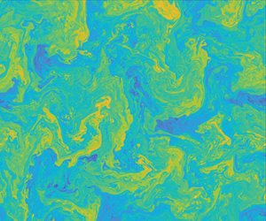
We first present some important features of the turbulent fields using the numerical results with  $\nu =10^{-16}$. Figure 1 shows snapshots of vorticity
  $\nabla ^2 \psi$ and two buoyancy fields. It is seen that the vertical buoyancy field
  $\theta$, which contains up- and down-moving plumes, just resembles the temperature field in the 2-D homogeneous RBC system (Celani et al. Reference Celani, Lanotte, Mazzino and Vergassola2000). However, it differs from the horizontal buoyancy field
  $\sigma$, where left- and right-moving plumes are present. Their difference can be seen from the asymmetry of sharp interfaces: in the
  $\theta$ field, the horizontal sharp interfaces prefer negative gradients of
  $\theta$, while the vertical interfaces consist of nearly symmetric positive and negative gradient of
  $\theta$; and vice versa for the
  $\sigma$ field. Thus the combination of
  $\theta$ and
  $\sigma$ leads to the present isotropic convection.

Figure 1. Snapshots of  $\nabla ^2\psi$,
  $\sigma$ and
  $\theta$ at a statistically steady state.
The isotropic feature of the turbulent fields is illustrated further in figure 2, where the second- and third-order isotropic fields, including  $\overline {\delta u^2}+\overline {\delta w^2}$,
  $\overline {\delta \sigma ^2}+\overline {\delta \theta ^2}$,
  $\boldsymbol {\nabla }\boldsymbol {\cdot } V_{K}$ and
  $\boldsymbol {\nabla }\boldsymbol {\cdot } V_{P}$, are plotted separately. As expected, all these fields show isotropic behaviours, which will be confirmed quantitatively later. Although anisotropy is present at large scales, owing to the effect of the square periodic box, the flows at these scales are dominated by large-scale damping and therefore do not affect the statistics at scales where BO scaling presents.

Figure 2. Isotropic fields of  $\overline {\delta u^2}+\overline {\delta w^2}$,
  $\overline {\delta \sigma ^2}+\overline {\delta \theta ^2}$,
  $\boldsymbol {\nabla }\boldsymbol {\cdot } V_{K}$ and
  $\boldsymbol {\nabla }\boldsymbol {\cdot } V_{P}$.
4.2. Low-order structure functions
In § 3.2, we discussed that the key for the BO scenario is associated with the transfer directions of the potential and kinetic energy. Here, we present the numerical evidence. Figure 3 shows the kinetic and potential energy fluxes, and their difference is also presented because the buoyancy terms in the kinetic and potential energy equations cancel. It is seen that the potential energy transfers downscale and the kinetic energy transfers upscale, thus supporting the assumption proposed in § 3.2. And the wide plateau appearing in their difference justifies not only the negligible effects of dissipation and diffusivity, but also the correctness of our simulations. We also compare the potential energy fluxes in simulations with different  $\nu$. It is seen that decreasing the hyperviscosity results in a wider range for the approximately constant potential energy flux, and therefore extends the possible range for detecting the BO scaling. In other words, the present isotropic convection system would exhibit the BO scaling more evidently with smaller hyperviscosities (equivalently, at larger
  ${{Ra}}$ values).

Figure 3. Kinetic ( $F_{K}$) and potential (
 $F_{P}$) energy fluxes, as well as their difference. Potential energy fluxes with different hyperviscosities are also plotted for comparison.
To verify the above discussion quantitatively, and most importantly the scaling relations (3.12) derived in § 3.3, we now check in figure 4 the third-order structure functions corresponding to the kinetic and potential energy fluxes. There exists a wide range of length scales in which the data closely follow the BO scaling. Moreover, the results in figure 4(b) show that the BO scaling range extends much further as the hyperviscosity decreases, confirming the discussion above. Here, the isotropic features of the present system are verified quantitatively by comparing the results in different directions. Similarly, the second-order structure functions shown in figure 5 also follow the BO scalings. In addition, the well-collapsed data for different directions and components further demonstrate the isotropy of the flow fields. Thus combining the information of figures 4 and 5, we can conclude safely that the BO scaling is well observed in the low-order structure functions of the present isotropic convection system.

Figure 4. The third-order structure functions corresponding to the kinetic and potential energy fluxes at different directions. The BO scalings are plotted for reference. Again, the data with different hyperviscosities are plotted in panel (b) for comparison.

Figure 5. The second-order structure functions of (a) velocity and (b) temperature fields for different components and directions. The BO scalings are plotted for reference.
4.3. High-order structure functions
In this section, we study the high-order structure functions. Because the flow fields well satisfy the isotropic condition, we focus on the statistics of the horizontal velocity  $u$ and the temperature field
  $\theta$. In figure 6, we plot the structure functions of
  $\delta u$ and
  $\delta \theta$ from order
  $2$ to order
  $9$, and the corresponding scaling exponents
  $\zeta _u$ and
  $\zeta _\theta$ (cf. (3.13a,b)) in the inertial range are also shown. Note that only the absolute values of
  $S_n^\theta$ are exhibited, as the high-order structure functions of
  $\theta$ can be negative. Figures 6(c,d) show the compensated plots of the ninth-order structure functions of
  $u$ and
  $\theta$, to show the quality of scaling behaviour. The compensated scaling
  $r^{27.3/5}$ in the velocity structure function is very close to the BO scaling
  $r^{27/5}$. A bottleneck effect (cf. Frisch et al. Reference Frisch, Kurien, Pandit, Pauls, Ray, Wirth and Zhu2008) is seen in the structure function of
  $\theta$, but the scaling recalls similar behaviour observed in 3-D isotropic turbulence by Haugen & Brandenburg (Reference Haugen and Brandenburg2004). The bottleneck effect is not seen in the velocity structure function; this is because the kinetic cascades upscale while the potential energy cascades downscale. The high-order structure functions do have power-function dependence on two-point distance. The non-intermittent BO scaling
  $\zeta _u = 3n/5$ (cf. (3.14a,b)) well captures the behaviour of the high-order velocity structure functions, but the temperature structure functions show strong intermittency. It is seen that the scaling exponent
  $\zeta _\theta$ deviates from the BO prediction (i.e.
  $\zeta _\theta = n/5$) and saturates to value 0.75 as
  $n\geq 5$, which is similar to the results in 2-D homogeneous RBC (Celani et al. Reference Celani, Matsumoto, Mazzino and Vergassola2002). However, an interesting observation is that
  $\overline {\delta \theta ^3} \sim r^{3/5}$, which was not shown in previous studies.

Figure 6. (a,b) Structure functions  $S_n^u$ and
  $S_n^\theta$ with
  $n=2,3,4,5,6,7,8,9$. The curves are shifted vertically. (c,d) Compensated ninth-order structure functions of
  $u$ and
  $\theta$, where the horizontal dashed lines are presented for reference. The power-function fittings to the data in the BO scaling range are also presented. (e, f) Corresponding scaling exponents
  $\zeta _u$ and
  $\zeta _\theta$.
The intermittent effects can be also observed in the p.d.f.s of, for example, the normalized longitudinal velocity increment  $\delta u_L$ and temperature increment
  $\delta \theta _L$, as shown in figure 7. Here,
  $\delta u_L$ is evaluated with the
  $x$-direction displacement, and
  $\delta \theta _L$ is evaluated with the
  $z$-direction displacement. It is seen that the p.d.f.s of
  $\delta u_L$ for different scales are well collapsed and all Gaussian-like, though the upscale energy transfer brings about positive skewness, which resembles that in the inverse cascade range of 2-D turbulence (cf. Boffetta, Celani & Vergassola Reference Boffetta, Celani and Vergassola2000; Boffetta & Ecke Reference Boffetta and Ecke2012). However, the p.d.f.s of
  $\delta \theta _L$ for different scales do not fall on top of each other, and their departure from the Gaussian distribution becomes much stronger at smaller scales, manifesting the effects of intermittency (Celani et al. Reference Celani, Mazzino and Vergassola2001).

Figure 7. P.d.f.s of normalized  $\delta u_L$ and
  $\delta \theta _L$;
  $r$ is the distance between two measured points. The black dashed line is the normal distribution for reference.
Figure 8 shows the integration kernels for the sixth- and eighth-order structure functions of  $u$ and
  $\theta$, which justify the convergence of high-order structure functions. Figures 8(a,b) show a larger probability of the positive velocity difference, which is in consistent with the positive third-order structure function
  $\overline {\delta u_L^3} > 0$ corresponding to an upscale kinetic energy flux shown in figure 3. This contrasts with the integration kernels observed in 3-D RBC with a forward kinetic energy cascade (cf. Sun et al. Reference Sun, Zhou and Xia2006). The collapse of integration kernels with different displacements again shows the non-intermittency of velocity differences. The integration kernels of temperature structure functions shown in figures 8(c,d) show a preference of negative values, which is in accord with the plumes structures (cf. figure 1). The hot plumes travel upwards and cold plumes travel downwards, so collisions of plumes give strong negative and weak positive
  $\theta$ gradients in the vertical direction. This negative-value preference is also observed in 3-D RBC (Sun et al. Reference Sun, Zhou and Xia2006). Different from the integration kernels of velocity difference, those of temperature difference with different displacements do not collapse, indicating strong intermittency, which is consistent with figure 7(b).

Figure 8. Integration kernels for the sixth- and eighth-order longitudinal structure functions of  $u$ and
  $\theta$ with different displacements of two measured points.
4.4. RBC in a periodic domain
To gain a better understanding of the present isotropic convection system, we compare it with the homogeneous RBC system, i.e. the canonical anisotropic RBC in a periodic domain. The simulation uses the same algorithm as for the isotropic system with  $\nu =10^{-16}$, but without the horizontal component in the buoyancy field. To obtain trustable statistics, we run the simulation to a statistically steady state and maintain for
  $8\times 10^4$ eddy turnover time, which is calculated as the inverse of the mean square vorticity. The convergence of the statistics has also been checked by calculating the integral kernels of structure functions (not shown here) as in figure 8.
Figure 9 shows some statistical quantities of the homogeneous RBC, which are the counterparts of those shown in figure 2. It is seen that even the second-order statistics have exhibited obvious anisotropic features, which elongate along the vertical direction as expected. When it comes to the third-order statistics, the anisotropy is more dramatic, resulting in the longitudinal and transversal structure functions being distinctive.

Figure 9. Isotropic fields of  $\overline {\delta u^2}+\overline {\delta w^2}$,
  $\overline {\delta \theta ^2}$,
  $\boldsymbol {\nabla }\boldsymbol {\cdot } V_{K}$ and
  $\boldsymbol {\nabla }\boldsymbol {\cdot } V_{P}$ in 2-D homogeneous (but anisotropic) RBC.
To further illustrate the impact of anisotropy, we show in figure 10 the third-order structure functions corresponding to kinetic and potential energy fluxes in different directions in the anisotropic RBC, which are the counterparts of those shown in figure 4. Figure 10(a) shows that both the horizontal and vertical components of the kinetic energy structure function deviate from the BO scaling, with a steeper scaling for the horizontal component and a shallower scaling for the vertical component. For the potential energy structure function, the vertical component is close to the BO scaling, while the horizontal component is shallower. The anisotropic behaviour of both the kinetic and potential energy third-order structure functions, which differ from the isotropic structure functions of our isotropic system (cf. figure 4), shows the anisotropic energy flux phenomenon in the homogeneous RBC.

Figure 10. The third-order structure functions corresponding to the kinetic and potential energy fluxes at different directions in anisotropic RBC. The BO scalings are plotted for reference.
The anisotropy traces back to instability, which drives the turbulent dynamics. In homogeneous RBC, the linear growth rate  $\lambda _{RBC}$ with respect to the zero state of (2.1a)–(2.1b) reads
 \begin{equation} \lambda_{RBC} = \frac{1}{2} \left( -(\nu_0+\kappa_0) K^2 + \sqrt{ (\nu_0+\kappa_0)^2 K^4 - 4\nu_0\kappa_0K^4 + \frac{4 g\beta k ^2}{K^2} } \right), \end{equation}
which is anisotropic. For horizontal modes with  $\boldsymbol {k} = (0,m)$, the growth rate
  $\lambda _{RBC}$ is negative, therefore these modes are linearly stable and do not inject energy into the system, while the most unstable mode is a so-called elevator mode with
  $m=0$. Therefore, it is expected to observe more flow structures – plumes – propagating vertically. So in figures 9(c,d), the divergence of third-order structure functions, which correspond to energy sources and sinks, concentrate around locations with zero vertical displacement. Considering that in the spectral space the nonlinear advection transfers energy from sources, where the modes are unstable, to sinks, the anisotropic growth rate (cf. (4.1)) leads to anisotropic energy transfer (cf. figure 10), which further leads to anisotropic structure functions in inertial ranges. It is this anisotropic energy transfer that contaminates the scaling behaviour in the canonical RBC. Note that an alternative way to analyse the anisotropy in turbulent flows is by examining structure functions with different symmetry (cf. Biferale & Procaccia Reference Biferale and Procaccia2005), which is beyond the scope of this paper.
5. Summary and discussion
In this paper, we construct a 2-D isotropic convection system in a doubly periodic domain, aiming to explore the BO scaling in a situation without any complicating factor that contaminates the scaling properties. The periodic domain avoids the impact of the walls and the large-scale circulations, and the 2-D formulation with upscale kinetic energy flux enables the observation of a long inertial range for the BO scenario. These advantages are shared with previous studies of 2-D homogeneous RBC (Biskamp & Schwarz Reference Biskamp and Schwarz1997; Biskamp et al. Reference Biskamp, Hallatschek and Schwarz2001; Celani et al. Reference Celani, Mazzino and Vergassola2001; Mazzino Reference Mazzino2017) and RT turbulence (Chertkov Reference Chertkov2003; Boffetta et al. Reference Boffetta, De Lillo, Mazzino and Musacchio2012). However, the turbulent fields in those systems are still anisotropic, making the scaling properties of structure functions depend on the evaluated direction, as we demonstrated in § 4.4. By introducing an extra buoyancy field subjected to horizontal gravity, we successfully obtain an isotropic convection system, which makes the structure functions directional-independent, and thus it is perfect to explore the BO scenario.
Based on the downscale flux of the potential energy and the upscale flux of the kinetic energy, we derive structure function relations from the KHM equations for the present isotropic convection system. And invoking self-similarity, these structure function relations lead directly to the BO scaling, which is checked with direct numerical simulations. It is found that the second- and third-order structure functions of velocity and buoyancy all follow the BO scaling. For high-order structure functions, the velocity field shows no intermittency, but the buoyancy field shows strong intermittency with the scaling exponent  $\zeta _\theta \to 0.75$ as the order
  $n \ge 5$. These results for high-order structure functions are similar to those observed in 2-D homogeneous RBC (Celani et al. Reference Celani, Matsumoto, Mazzino and Vergassola2002; Mazzino Reference Mazzino2017), while in 2-D RBC,
  $\zeta _\theta$ tends to a value (
 ${\sim }0.8$) slightly larger than
  $0.75$. The major difference is that the third-order structure function of buoyancy in the isotropic convection follows the BO scaling perfectly, contradicting the result in homogeneous RBC. We believe that this difference stems from the isotropy as discussed in § 4.4.
We end this paper by noting the key for detecting the BO scaling, which has been conjectured to be associated with the inverse kinetic energy cascade (Boffetta et al. Reference Boffetta, De Lillo, Mazzino and Musacchio2012). Although some RBC experiments on soap films/bubbles have reported BO-like scaling, the direction of the kinetic energy flux in these studies was unclear (Zhang & Wu Reference Zhang and Wu2005; Seychelles et al. Reference Seychelles, Ingremeau, Pradere and Kellay2010). Thus our theoretical argument and numerical results provide direct support for the validity of this conjecture in RBC. While the present 2-D isotropic convection is physically unrealizable, the realization of inverse kinetic energy cascade in a laboratory is quite feasible. One promising approach is to use geometrical confinement, i.e. a quasi-2-D system, as Boffetta et al. (Reference Boffetta, De Lillo, Mazzino and Musacchio2012) did in the study of RT turbulence. Some recent studies of quasi-2-D RBC have observed the condensation of turbulent structures (Huang et al. Reference Huang, Kaczorowski, Ni and Xia2013; Chong et al. Reference Chong, Huang, Kaczorowski and Xia2015), which is an intriguing feature due to the inverse kinetic energy cascade (Xia et al. Reference Xia, Byrne, Falkovich and Shats2011). In this context, the present 2-D system is also worthwhile to extend to its counterparts in quasi-2-D and 3-D systems, which may help to reveal the connection between 2-D and 3-D RBC in terms of small-scale statistics. We expect that the present 2-D isotropic convection can not only improve theoretical understanding of canonical RBC, but also stimulate experiments that go beyond the canonical RBC configuration, which is exactly the current trend in the field of turbulent convection (Xia Reference Xia2013).
Acknowledgement
The authors thank K.-Q. Xia for helpful discussions.
Funding
J.-H.X. gratefully acknowledges financial support from the National Natural Science Foundation of China (NSFC) under grant no. 92052102, and the Joint Laboratory of Marine Hydrodynamics and Ocean Engineering, Pilot National Laboratory for Marine Science and Technology (Qingdao). S.-D.H. is supported by the NSFC (grant nos 11988102, 11961160719 and 91752201) and the Department of Science and Technology of Guangdong Province (grant no. 2019B21203001).
Declaration of interests
The authors report no conflict of interest.
Appendix A. Statistics of some other isotropic quantities
In this appendix, we study the structure functions of some isotropic scalars that are non-intermittent. Due to the presence of a horizontal buoyancy field, we can introduce two isotropic scalar quantities, namely  $\varPsi$ and
  $\varPhi$, through the Helmholtz decomposition of buoyancy fields, as
 \begin{equation} (\sigma,\theta) = \boldsymbol{\nabla}\varPhi + \boldsymbol{\nabla}^\perp\varPsi. \end{equation}
 It is natural to study their structure functions together with the streamfunction  $\psi$. Based on the discussion in § 3, a simple dimensional analysis implies that
 \begin{equation} \delta\psi \sim r^{8/5} \quad \mathrm{and} \quad \delta\varPhi \sim \delta\varPsi \sim r^{6/5}, \end{equation}
which, however, is problematic. This is because, for the second-order statistics, we have
 \begin{equation} \nabla^2\overline{\delta \psi^2} = 2(\overline{u^2}+\overline{w^2} - \overline{\delta u^2} - \overline{\delta w^2}). \end{equation}
As  $\overline {\delta u^2} + \overline {\delta w^2} \sim r^{6/5}$ follows the BO scaling, we immediately obtain
 \begin{equation} \overline{\delta \psi^2} \sim r^2 + {\rm h.o.t.} \end{equation}
when considering the small- $r$ limit, which is in contrast to (A2a,b). Note that (A4) holds as long as the scaling exponent of
  $\overline {\delta u^2} + \overline {\delta w^2}$ is positive. However, the high-order structure functions of
  $\delta \psi$ do not have relations like (A3) that are linked to the structure functions of
  $\delta u$, so their scalings are unknown. Nevertheless, according to (A4), a naive guess for the
  $n$th-order structure functions of
  $\delta \psi$ (without intermittency) is
 \begin{equation} \overline{\delta \psi^n} \sim r^n. \end{equation}
Similarly, the structure functions of  $\delta \varPsi$ and
  $\delta \varPhi$ for the leading order are expected to be
 \begin{equation} \overline{\delta \varPsi^n} \sim r^n \quad \mathrm{and} \quad \overline{\delta \varPhi^n} \sim r^n. \end{equation}
 Now we use the numerical data to check the scaling relations (A5) and (A6a,b). In figure 11, we show the structure functions of  $\psi$,
  $\varPsi$ and
  $\varPhi$ for different orders, together with their scaling exponents obtained in the inertial range. For the structure functions of
  $\psi$ and
  $\varPsi$, we plot their absolute values, but for the structure functions of
  $\varPhi$, we plot the positive and negative parts separately due to their different scaling behaviours. It is seen that all the structure functions exhibit power-function dependencies and no intermittency is observed, but their scaling exponents are distinctive. To be specific, while the scaling exponents
  $\zeta _\psi$ of the structure functions of
  $\psi$ follow (A5) nicely, those for the structure functions of
  $\varPsi$ show a non-expected dependence as
  $\zeta _\varPsi = 9n/10$. Note that even for
  $n=2$,
  $\zeta _\varPsi$ differs from the prediction given by (A6a,b), though their differences are not that much. More interestingly, the positive and negative parts of the structure functions of
  $\varPhi$ exhibit different scalings. While the scalings for the positive part also follow a dependence as
  $\zeta _{\varPhi +} = 9n/10$, those for the negative part have a more strange behaviour as
  $\zeta _{\varPhi -} = 6/5+4n/5$. We do not have an explanation for the behaviour of these scaling exponents, which is subject to future study.

Figure 11. Structure functions of (a,c,e,g)  $\psi$,
  $\varPsi$ and
  $\varPhi$ and (b,d, f,h) their scalings. The absolute values of structure functions of
  $\psi$ and
  $\varPsi$ are presented as
  $S_n^\psi$ and
  $S_n^\varPsi$, respectively. Here,
  $S_n^{\varPhi +}$ and
  $S_n^{\varPhi -}$ denote the positive and negative parts of the structure functions of
  $\varPhi$.


