


1. Introduction
When two concentric spherical shells are differentially rotated, the fluid layer contained between these spheres is sheared, generating vortical fluid motion. In the subsurface oceans of Jupiter's and Saturn's icy moons, it is thought that extremely vigorous motion is driven by the differential rotation of the ice shell and rocky core, and that the viscous dissipation may play a role in maintaining the ocean's liquid state (Peale, Cassen & Reynolds Reference Peale, Cassen and Reynolds1979; Tyler Reference Tyler2008; Nimmo & Pappalardo Reference Nimmo and Pappalardo2016; Wilson & Kerswell Reference Wilson and Kerswell2018). Covering these tidally heated oceans is an ice shell, which, particularly for deeper shells, is suspected to convect thermally (McKinnon Reference McKinnon1999; Barr & McKinnon Reference Barr and McKinnon2007; Mitri & Showman Reference Mitri and Showman2008). A role of the ice and ocean layer in these systems is therefore to increase the transfer of both angular momentum and heat, although, as we shall demonstrate, the motion favoured by each driving mechanism differs. The competition between these nonlinear effects results in a system with bistable solution states.
Bistability or multistability (Feudel, Pisarchik & Showalter Reference Feudel, Pisarchik and Showalter2018), has been observed in numerical simulations (Mamun & Tuckerman Reference Mamun and Tuckerman1995) and experiments of the laminar (Wimmer Reference Wimmer1976; Bühler Reference Bühler1990) and turbulent (Zimmerman, Triana & Lathrop Reference Zimmerman, Triana and Lathrop2011) flow between differentially rotating spheres. It is also observed in experiments with turbulent flow between differentially rotating cylinders (Huisman et al. Reference Huisman, van der Veen, Sun and Lohse2014; van der Veen et al. Reference van der Veen, Huisman, Dung, Tang, Sun and Lohse2016) and for a cylinder with rotating end caps (Ravelet et al. Reference Ravelet, Marié, Chiffaudel and Daviaud2004). In each of these configurations, cellular flows are generated to transport angular momentum, although neither experiments or computations indicate that the flow chooses the state which maximise its torque. Zimmerman et al. (Reference Zimmerman, Triana and Lathrop2011) attributes bistability to the formation and destruction of resilient zonal flows such as jets, while Wimmer (Reference Wimmer1976) attributes it to the centrifugal forces responsible for instabilities in rotating spheres which vary with latitude.
For thermal convection in spherical shells, multistability has also been demonstrated numerically (Li et al. Reference Li, Zhang, Liao and Zhang2005; Feudel et al. Reference Feudel, Bergemann, Tuckerman, Egbers, Futterer, Gellert and Hollerbach2011) and experimentally (Travnikov et al. Reference Travnikov, Zaussinger, Beltrame and Egbers2017). In this scenario, the high degree of symmetry in a spherical domain permits a number of subspaces, or basins of attraction. Provided perturbations of the laminar state remain sufficiently small, these basins of attraction are not explored and the flow remains stable, but for larger Rayleigh numbers  $Ra > 10^4$ this is not always the case (Huisman et al. Reference Huisman, van der Veen, Sun and Lohse2014). Experimental and numerical simulations in long cylinders, show that a large scale circulation or mean wind alternates between two states, and that the relative time spent in each state may be controlled by varying the aspect ratio (Xi & Xia Reference Xi and Xia2008; van der Poel, Stevens & Lohse Reference van der Poel, Stevens and Lohse2011; Weiss & Ahlers Reference Weiss and Ahlers2013). This behaviour has also been demonstrated experimentally in a rectangular box by Sreenivasan, Bershadskii & Niemela (Reference Sreenivasan, Bershadskii and Niemela2002) who proposed a physical model for this behaviour, and related the alternation of its mean wind to the concept of self-organised criticality (Jensen Reference Jensen1998).
In summary, bistable behaviour is observed in both laminar and turbulent flows, where the transfer of heat and angular momentum is of importance. As this phenomenon is of particular relevance in planetary systems, we attempt to explain how this can occur by focusing on a model system where both effects are present.
1.1. Description of physical processes
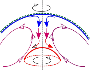
In figure 1(a) the fluid motion arising due to differential rotation of the spheres (with angular velocities  $\omega_1 \!\neq \omega_2$ and radii
  $r_1,r_2$) is sketched. This configuration is also known as spherical Couette flow (Marcus & Tuckerman Reference Marcus and Tuckerman1987a,Reference Marcus and Tuckermanb). The differential rotation shears the flow imparting angular momentum to the fluid. Since the annular domain is closed, the fluid is forced to recirculate so that for small rotation rates, as characterised by the inner sphere Reynolds number
  $Re_1 = \omega _1 r^2_1/\nu$, the resulting imbalance generates a large scale flow containing two cells. These cells tend to localise about the equator where the velocity is greatest, establishing a radial inflow or outflow in the direction of decreasing angular momentum. In figure 1(a) this is an equatorial outflow as
  $\omega _1 > \omega _2$.

Figure 1. Schematic of the anticipated fluid flow in a spherical annulus due to differential rotation (shear) or a destabilising thermal gradient (buoyancy). (a) Inner sphere rotation establishes a cellular pattern of fluid motion, originating from the need to transport high angular momentum fluid outwards at the equator, where the sphere's velocity is greatest. (b,c) Thermal convection can establish even or odd cellular patterns depending on the annulus width. Cells transport lighter hot fluid outwards and draw cooler fluid inwards. (a) Couette flow, (b) even convection and (c) odd convection.
In figures 1(b) and 1(c) the behaviour of thermal convection is shown schematically. When the ratio of buoyancy to viscous forces as characterised by the Rayleigh number  ${Ra}$ becomes sufficiently large, a cellular flow succeeds the conductive state. In this convecting state hotter fluid with a lower density rises while colder heavier fluid sinks under the action of gravity. This behavioural tendency was first outlined theoretically by Rayleigh (Reference Rayleigh1916) who demonstrated that a fluid layer heated from below becomes unstable to two-dimensional (2-D) rolls with a definite horizontal wavenumber. Similarly in a spherical shell, a different number of cells will occupy the annulus depending on the separation
  $d$ between the spheres. This is shown schematically in (b,c) of figure 1 where an even two-cell and odd three-cell flow are depicted. Distinct from spherical Couette flow, thermal convection can establish either an equatorial inflow or outflow. In addition, the cellular convecting state arises from a thermal instability while in spherical Couette flow it is present for all
  $Re_1 \neq 0$.
Astrophysical studies of rotating convection typically focus on the case of rapid co-rotation where the dominant physical balances are between the Coriolis and buoyancy forces (Zhang & Liao Reference Zhang and Liao2017). In this regime rotation tends to stabilise the flow such that it arranges itself in concentric layers of fluid known as Taylor columns (Proudman & Lamb Reference Proudman and Lamb1916). Uniform rotation is then the dominant effect, and variations in the rotation rate appear as perturbations. Although this is the most relevant configuration for the subterranean oceans of Jupiter's and Saturn's moons (Wilson & Kerswell Reference Wilson and Kerswell2018), in their ice shells it is buoyancy and viscous forces which take precedence (McKinnon Reference McKinnon1999). As shown in appendix A, azimuthal shear is then dynamically significant. In this paper, we consider viscous thermal convection with a stationary outer sphere and rotating inner sphere  $(\omega _2 = 0, \omega _1 \neq 0)$ in order to accentuate the effect of differential rotation. This configuration is chosen with the purpose of understanding how the flow facilitates the transport of angular momentum and heat, as the strength of the temperature gradient
  $Ra$ and differential rotation
  $Re_1$ increase. According to the Rayleigh criterion (Taylor Reference Taylor1923) rotating the inner sphere (or counter-rotating the spheres) is the least stable configuration. Therefore, we anticipate that when
  $\omega _2 = 0$ the flow is likely to transition to a more complicated state at smaller values of
  $Ra, Re_1$. In § 4 we present numerical simulations which confirm this assumption and indicate that including co-rotation does not modify our findings significantly. Fixing
  $Re_2=0$ also provides a welcome reduction in the parameter space to be studied.
1.2. Prior work and the axisymmetric assumption
To the authors’ knowledge four works have previously studied this configuration. Yanase, Mizushima & Araki (Reference Yanase, Mizushima and Araki1995) and Araki, Yanase & Mizushima (Reference Araki, Yanase and Mizushima1996) allow for rotation of the inner sphere with fixed Prandtl number  ${\textit {Pr}} = 7$ and separation
  $d=0.45$. Assuming the system is axisymmetric and by artificially enforcing equatorial symmetry, they numerically solve for even solutions only. Loukopoulos (Reference Loukopoulos2004) also studied the axisymmetric system numerically, but allowed for equatorial asymmetry and axial gravity in contrast to Yanase et al. (Reference Yanase, Mizushima and Araki1995) and Araki et al. (Reference Araki, Yanase and Mizushima1996). Varying
  $Ra$, while keeping
  ${{\textit {Pr}}=}1, d=0.18$ and
  $Re_1$ fixed, asymmetric solutions and the transitions towards a solution state with a progressively larger number of Taylor vortices was reported.
Recently Inagaki, Itano & Sugihara-Seki (Reference Inagaki, Itano and Sugihara-Seki2019) considered the fully 3-D problem for fixed  ${\textit {Pr}} = 1,d=1$. Numerically they showed that the axisymmetric two-cell solution (cf. figure 1a,b) is preferred for a large range of
  $(Re_1,Ra)$ parameter space. Their stability diagram, although not always easy to follow, indicates that the
  $Ra$ at which the onset of 3-D convection occurs increases with
  $Re_1$, while for large
  $Re_1 \approxeq 500$ it is reduced. In addition they showed that increasing
  $Re_1$ for fixed
  $Ra$, induces the transition to a non-axisymmetric state, but that the resulting transition does not necessarily increase the torque or heat transfer.
This paper is structured as follows. After outlining the governing equations in § 2, we investigate how the onset of both even and mixed/odd convection is modified by the presence of weak inner sphere rotation in § 3. In this section we also outline how  ${\textit {Pr}}$ and system symmetries influence whether the transition from an even to odd number of cells exhibits hysteresis. Fixing
  ${\textit {Pr}} =10,d = 3$ in § 4, we outline all possible solutions in
  $Re_1,Ra$ space, and to understand the physical mechanisms underlying the transition between different solutions examine their least stable perturbations. In § 5 we validate our restriction to axisymmetry by computing the stability of axisymmetric states to non-axisymmetric disturbances. Finally in § 6 we summarise the main results.
2. Formulation of the problem
As shown in figure 2, we consider convection in a spherical annulus of separation  $d = (r_2 - r_1)/r_1$ allowing for differential rotation of the spheres
  $\omega _1 \neq \omega _2$. Constant temperatures
  $T_1, T_2$ are prescribed at the spheres’ boundaries, with difference
  ${\rm \Delta} T = T_1 - T_2 > 0$. We assume a Boussinesq fluid with density
  $\rho _f$ that varies linearly with temperature fluctuations according to the relation
 \begin{equation} \rho = \rho_f [1 + \hat{\beta} (T_0(r) - T(r,\theta,t) ) ], \end{equation}
where the thermal expansion coefficient  $\hat {\beta }$ is small and
  $T_0(r)$ is the conductive base state. The spherically symmetric gravity field is expressed as
 \begin{equation} \boldsymbol{g} = -g_0 g(r) \boldsymbol{r} = -\frac{g_0 r^2_1}{r^3} \boldsymbol{r}, \end{equation}
where  $g_0$ is the acceleration due to gravity on the inner sphere's surface. Choosing the length scale
  $r_1$, thermal diffusion time scale
  $r^2_1/\kappa$ and
  ${\rm \Delta} T$ as the temperature scale, the governing Oberbeck–Boussinesq equations may be written non-dimensionally as
 \begin{gather} \frac{1}{{\textit{Pr}}} \left( \frac{D \boldsymbol{u}}{D t} + \boldsymbol{\nabla} p \right) = Ra \, g(r) \boldsymbol{r} T + {\nabla}^2 \boldsymbol{u}, \end{gather}
 \begin{gather}\frac{\partial T}{\partial t} + \boldsymbol{u} \boldsymbol{\cdot} \boldsymbol{\nabla} T = \nabla^2 T,\quad \boldsymbol{\nabla} \boldsymbol{\cdot} \boldsymbol{u} = 0, \end{gather}
where  $p$ contains pressure- and gradient-like terms,
  ${\textit {Pr}}$ is the Prandtl number and the strength of the thermal gradient is characterised by the Rayleigh number
  $Ra$. In addition, we specify no-slip boundary conditions for
  $\boldsymbol {u}$ and assume perfectly conducting spherical shells for
  $T$ at the spherical walls
 \begin{equation} \left.\begin{aligned} \boldsymbol{u}(r = 1,\theta, \varphi) & = Re_1 {\textit{Pr}} \sin \theta \hat{\boldsymbol{\varphi}}, \quad \boldsymbol{u}(r = 1 + d, \theta, \varphi) = Re_2 Pr \sin \theta \hat{\boldsymbol{\varphi}}\\ T(r=1,\theta,\varphi) & = 1, \quad T(r=1+d,\theta,\varphi) = 0, \end{aligned}\right\} \end{equation}
such that the strength of the differential rotation is defined by  $|Re_1 - Re_2|$. Unless otherwise stated, it can be assumed that
  $Re_2 = 0$ for the remainder of this paper. For reference, it is convenient to define the following parameters:
 \begin{equation} \left.\begin{aligned} {\textit{Pr}} & = \nu/\kappa\\ {Ra} & = \frac{g_0 \hat{\beta} {\rm \Delta} T\; r_1^3}{\nu \kappa} \\ Re_1 & = \frac{\omega_1 r^2_1}{\nu} \end{aligned}\right\} \begin{aligned} \text{Prandtl Number} \\ \text{Rayleigh Number} \\ \text{Reynolds Number}. \end{aligned} \end{equation}
Figure 2. The fluid domain is a closed annular region between two concentric spheres, of radii  $r_1,\ r_2$. Each sphere maintains a constant surface temperature
  $T_1,\ T_2$, rotating with angular velocities
  $\omega _1,\ \omega _2$ respectively. Gravity
  $\boldsymbol {g}$ acts radially inward. The inner core has a density
  $\rho _c$ and the fluid annulus
  $\rho _f$.
We begin by assuming that all longitudinal variations  $\partial /\partial \varphi = 0$, and concentrate primarily on the axisymmetric system
 \begin{align} \boldsymbol{u} = \boldsymbol{\nabla} \times \left(0,0,\frac{\psi}{r \sin \theta}\right) + \left( 0,0, \frac{\varOmega}{r \sin \theta} \right) = \left( \frac{1}{r^2 \sin \theta} \frac{\partial \psi}{\partial \theta}, \frac{-1}{r \sin \theta}\frac{\partial \psi}{\partial r}, \frac{\varOmega}{r \sin \theta} \right),\end{align}
such that the axisymmetric flow  $\boldsymbol {u}$ is described by a streamfunction
  $\psi (r,\theta ,t)$ and specific angular momentum
  $\varOmega (r, \theta , t)$. We do not, however, discount the possibility of non-axisymmetric motions. We first solve for axisymmetric solutions of (2.3) and subsequently compute their stability to 3-D perturbations. In this manner, we determine whether a given axisymmetric solution represents a stable 3-D state. This approach is motivated by numerical simulations of the fully 3-D system (Inagaki et al. Reference Inagaki, Itano and Sugihara-Seki2019) and by experiments and numerical simulations of isothermal spherical Couette flow (Junk & Egbers Reference Junk and Egbers2000; Hollerbach, Junk & Egbers Reference Hollerbach, Junk and Egbers2006). Both scenarios show that the flow remains axisymmetric for moderate
  $Re_1$. In addition, the axisymmetric case is easier to treat both analytically and numerically, and represents an appropriate starting point from which valuable insights can be obtained.
Substituting (2.6) into (2.3), a set of coupled equations for  $\psi ,T,\varOmega$ are obtained. In the following sections these equations are analysed using direct numerical simulation (DNS). Their discretisation, outlined in Mannix (Reference Mannix2020), uses a Galerkin projection in terms of Legendre
  $P_{\ell }(\cos \theta )$ and Gegenbauer
  $G_{\ell }(\theta ) = \sin \theta \partial _{\theta } P_{\ell }(\cos \theta )$ polynomials to treat the
  $\theta$ dependency exactly following Mavromatis & Alassar (Reference Mavromatis and Alassar1999). Evaluating the triple integrals which arise in this formulation is facilitated by the method of Johansson & Forssén (Reference Johansson and Forssén2016). A Chebyshev collocation method is used to treat their radial dependency (Trefethen Reference Trefethen2000). A limitation of this method is its high numerical complexity
  $\sim {O}(N_{\theta }^3)$, where
  $N_{\theta }$ is the number of polynomials used, thus restricting our computations to cases where moderate
  $N_{\theta }$ provides adequate resolution. In the most demanding cases considered we have used
  $N_r = 50,\ N_{\theta } = 60$. This ensures that our truncated Chebyshev coefficients remain at most
  $ {O}(10^{-5})$, while polar coefficients are
  $ {O}(10^{-8})$ and
  $ {O}(10^{-3})$ for equatorially asymmetric and symmetric solutions respectively. The difficulties encountered in resolving the symmetric flow are attributed to thin thermal layers, which arise in the neighbourhood of the equator. Time stepping, steady-state solving and linear stability analysis are performed following Mamun & Tuckerman (Reference Mamun and Tuckerman1995). Numerical continuation is implemented using a weighted pseudo-arc length method following Uecker, Wetzel & Rademacher (Reference Uecker, Wetzel and Rademacher2014), while the continuation of bifurcation points is implemented following Kuznetsov (Reference Kuznetsov2004). In addition to this spectral code, an additional code which uses second-order finite differences in both spatial directions has also been used. We have been able to reproduce the results presented in this paper using both codes.
2.1. Base states
When  $Re_1 = 0$ we obtain the thermal convection problem. In this case, the temperature equation admits the purely conductive base state
  $T_0(r)$, which is obtained by solving
  $\nabla ^2 T = 0$ with boundary conditions (2.4). This yields
 \begin{equation} \frac{\textrm{d} T_0}{\textrm{d} r} = \frac{A_T}{r^2},\quad T_0 = A_T/r + B_T,\quad A_T = \frac{1+d}{d},\quad B_T = -\frac{ 1}{d}, \end{equation}
implying that temperature gradients are greatest near the inner sphere's surface. For  $Ra = 0$ and
  $Re_1 \ll 1$, (2.3) admit a Stokes solution
  $\varOmega _0(r, \theta )$ which is obtained by solving
  $D^2 \varOmega = 0$ with boundary conditions (2.4) giving
 \begin{equation} \left.\begin{aligned} \varOmega & = {\textit{Pr}} Re_1 \varOmega_0(r,\theta) + {O}({\textit{Pr}} Re_1^3) = {\textit{Pr}} Re_1 \left( \tilde{a} \, r^2 + \frac{\tilde{b}}{r} \right) G_1(\theta) + {O}({\textit{Pr}} Re_1^3), \\ \psi & = {\textit{Pr}} Re_1^2 \psi_0(r,\theta) + {O}({\textit{Pr}} Re_1^4) = {\textit{Pr}} Re_1^2 f(r) G_2(\theta) + {O}({\textit{Pr}} Re_1^4), \end{aligned}\right\}\end{equation}
where
 \begin{equation} \tilde{a} = \frac{1}{(1+d)^3 -1}, \quad \tilde{b} = \frac{- (1+d)^3 }{(1+d)^3 -1}, \end{equation}
and  $f(r)$ is a known quintic polynomial (Munson & Joseph Reference Munson and Joseph1971a,Reference Munson and Josephb). Notably, this base state is not a simple function of a single spatial variable but instead depends on both
  $r$ and
  $\theta$. This leads to a cellular background flow
  $\psi (r,\theta )$ for all non-zero
  $Re_1$, as shown in figure 3(a). It is because this cellular flow always exists for non-zero rotation, rather than arising from an instability, that makes the analysis of this convection problem non-standard.

Figure 3. Decoupled steady-state solutions of the differential rotation and thermal convection ( ${\textit {Pr}}=10$) problems illustrating similar spatial solutions. (a) Differential rotation (2.8) for
  $Re_1 =1,d =3, Ra = 0$. A two-cell poloidal flow
  $\psi _0$ transports fluid near the inner sphere with high specific angular momentum (shown as yellow in the
  $\varOmega _0$ field) outwards. (b) Two-cell thermal convection
  $Re_1 = 0,d=3,Ra = 740$, (c) three-cell thermal convection
  $Re_1 =0, d=1.8,Ra=2160$. Hot fluid near the inner sphere is convected outwards by a cellular flow
  $\psi$. For the convection problem
  $Ra \neq 0$, the number of cells as specified by the annulus width increases as
  $d$ reduces; (a)
  $\psi _{max,min} = ( 0.07,-0.07)$, (b)
  $\psi _{max,min} = ( 2.72,-2.72)$ and (c)
  $\psi _{max,min} = ( 2.80,-3.93)$.
2.2. Decoupled steady solutions
As shown schematically in figure 1, fluid motion (vorticity) in this model can be maintained by two distinct processes: buoyancy forces, which drive thermal convection when the conductive state becomes unstable, and differential rotation (wall shear), which drives a recirculating flow. Decoupled solutions of (2.3) for each process are shown in figure 3, where it is noteworthy that the contours of poloidal motion  $\psi$ in panels (a,b) have a qualitatively similar spatial form. While a poloidal flow
  $\psi _0$ is generated for all
  $Re_1 \neq 0$, thermal convection arises from an instability of the conductive base state (2.7a–d) when the
  $Ra$ exceeds a critical Rayleigh number termed
  $Ra_c$. The solutions shown in panels (b,c) are therefore simulated at a supercritical Rayleigh number
  $Ra > Ra_c$.
In the left half panel of figure 3(a) the specific angular momentum field  $\varOmega _0$ corresponding to the Stokes solution (2.8) for
  $Re_1 = 1$ is shown. In panels (b,c), the temperature field
  $T$ produced using DNS is shown. The corresponding poloidal flow field in terms of
  $\psi$ is also shown on the right-hand side of each panel. Focusing on panel (a) we see that the effect of inner sphere rotation is to generate a radial gradient of
  $\varOmega$ that is strongest at the equator where the sphere's velocity is greatest. The fluid responds by generating a two-cell poloidal flow
  $\psi _0$, which transports fluid near the inner sphere with high specific angular momentum
  $\varOmega _0$ outwards at the equator. In panels (b,c) an analogous situation arises, with hot fluid near the inner sphere convected outwards by a cellular poloidal flow
  $\psi$. Notably, the number of cells is determined by the annulus width
  $d$, so that by reducing
  $d$ in panel (c) the number of cells has increased. This contrasts with the behaviour of the flow shown in panel (a), where a two-cell flow is generated independent of
  $d$ provided
  $Re_1$ is not too large.
Given equations (2.3) with boundary conditions (2.4) and the knowledge that the two physical mechanisms driving the fluid flow yield distinct solution regimes, we numerically answer the following questions in § 3. In addition to the rotating and thermal convection solution regimes outlined, is there an intermediary regime where a mixed state exists? If so, how does the Prandtl number  ${\textit {Pr}}$ influence the solution state obtained and the type of transition observed? While § 3 only indirectly influences our main conclusions, we believe that by outlining the role of symmetries and
  ${\textit {Pr}}$ for simple transitions, a potential physical mechanism for hysteresis is made clearer.
3. The role of  ${\textit {Pr}}$ in hysteresis transitions

To understand how differential rotation alters the cellular pattern selected by thermal convection we consider two values of the annulus separation for a range of  ${\textit {Pr}}$. The value
  $d=3$ is chosen to ensure that thermal convection selects a two-cell flow and conversely
  $d=1.8$ is chosen so that an odd three-cell flow is selected. The choice of a wide annulus favouring low wavenumbers is also motivated by simplicity. Numerically fewer modes are required to resolve wider annuli and the presence of a similar spatial structure of the flows facilitates qualitative interpretations. From now on we refer to solutions qualitatively similar to the left-hand side of panel (a) of figure 3 as rotating solutions and those qualitatively similar to (b,c) as convective solutions.
3.1. Even solutions $d=3$

Figure 4 shows how the bifurcation of the conductive state to a state of even convection is altered by rotation of the inner sphere. In these bifurcation diagrams and those which follow, the L2 norm of the streamfunction as defined by
 \begin{equation} \|\psi\| = \text{sign}[u_r(r=1+d/2,\theta)]\sum_{\ell=1}^{N_{\theta}} \|\psi_{\ell}(r)\|, \end{equation}
is used as a solution measure. In selected bifurcation diagrams,  $\|\psi \|$ is multiplied by the sign of the radial velocity
  $u_r$ at the equator to demonstrate branching symmetry.

Figure 4. Splitting of the pitchfork bifurcation due to differential rotation is more pronounced for larger  ${\textit {Pr}}$. The figure shows the bifurcation of the conductive state to even thermal convection for different
  $Re_1$ and
  ${\textit {Pr}}$. Solid lines denote stable equilibria while dashed lines denote unstable equilibria. When
  $Re_1 \neq 0$ the symmetric pitchfork is split into two branches: a rotation dominated branch with positive radial velocity at the equator
  $u_r^+$ which emerges continuously from the conductive state and a convection dominated branch with negative radial velocity at the equator
  $u_r^-$; (a)
  ${\textit {Pr}} = 0.1$, (b)
  ${\textit {Pr}} = 1$ and (c)
  ${\textit {Pr}} = 10$.
Solutions for different  $Re_1$ are shown for three values of
  $Pr$ in figure 4. When
  $Re_1 = 0$, the conductive basic state
  $T_0(r)$ loses stability at a critical Rayleigh number
  $Ra_c$ through a pitchfork bifurcation. For
  $Re_1 \neq 0$, the pitchfork is split and becomes an imperfect pitchfork bifurcation, as shown in figure 4. The branches with positive equatorial velocity
  $u_r^+$ resembling the rotating solution connect continuously to the conductive state, while those with negative velocity
  $u_r^-$ resembling the convective solution emerge from a saddle-node bifurcation. The distance of this saddle-node bifurcation from the point
  $(Ra_c, \| \psi \| =0)$ is observed to increase with both
  $Re_1$ and
  ${\textit {Pr}}$. For small
  ${\textit {Pr}}$ the pitchfork is slightly deformed while for larger
  ${\textit {Pr}}$ the role of rotation begins to dominate. Similarly for larger rotation rates
  $Re_1 = 10$ the bifurcation is further deformed as shown in figure 4(c), such that the lower convection branches are longer found within the range investigated.
Fixing  $(Ra -Ra_c)/Ra_c = 0.5$ and performing continuation in
  $Re_1$ we find that only the rotating branch persists for large
  $Re_1$ as shown in figure 5. Starting on the
  $u_r^-$ branch and increasing
  $Re_1$ causes a transition to the
  $u_r^+$ branch, but decreasing
  $Re_1$ does not lead to the backwards transition. The system is bistable but not hysteretic. Comparing figures 5(a) and 5(b), we observe that the
  $u_r^-$ solution persists for a larger interval of
  $Re_1$ when
  ${\textit {Pr}}$ is smaller. Similarly, the amplitude of the rotating branch increases at a faster rate for large
  ${\textit {Pr}}$.

Figure 5. Symmetric solution states are bistable but do not exhibit hysteresis. Transition between the rotating branch  $u_r^+$ and the convection branch
  $u_r^-$ for
  $(Ra -Ra_c)/Ra_c = 0.5$. At
  $Re _1 = 0$ the
  $u_r^+,\ u_r^-$ solution branches are approximately equal, but for sufficient
  $Re_1$ the
  $u_r^-$ convection branch terminates in a saddle-node bifurcation and transitions to the rotating state. As rotation in both directions is equivalent when the outer sphere is fixed, only half the axis (
 $Re_1 > 0$) is shown in (b); (a)
  ${\textit {Pr}} = 1$ and (b)
  ${\textit {Pr}} = 10$.
Figures 6(a) and 6(b) show the corresponding spatial solutions of the branches in figure 4 at  ${\textit {Pr}} = 0.1,10$. To illustrate the different coupling regimes present at high and low
  ${\textit {Pr}}$ we have shown solutions at
  ${\textit {Pr}} = 0.1$ on the left half of each panel and solutions at
  ${\textit {Pr}} = 10$ on the right half of each panel. The poloidal two-cell flow
  $\psi$ remains qualitatively consistent in all cases, although its amplitude changes. Comparing the temperature and specific angular momentum (
 $T,\varOmega$) for each case, however, the differences in these flows are made evident.

Figure 6. Gradients of  $\varOmega$ are strongly advected by the poloidal flow for
  ${\textit {Pr}} \ll 1$ and gradients of
  $T$ for
  ${\textit {Pr}} \gg 1$. This figure shows steady equilibrium solutions for
  $Re_1 = 1,\ (Ra -Ra_c)/Ra_c = 0.5$ demonstrating different coupling regimes of the
  $u_r^+$ (a) and
  $u_r^-$ (b) solutions at high
  ${\textit {Pr}} = 10$ right half image and low
  ${\textit {Pr}} = 0.1$ left half image.
Considering the rotating branch  $u_r^+$ shown in figure 6(a), we see that, for
  ${\textit {Pr}} = 0.1$, the contours of
  $T$ are weakly deformed from concentric circles, but that gradients of
  $\varOmega$ are strongly advected by the poloidal motion. Conversely, we see that, for
  ${\textit {Pr}} = 10$, gradients of
  $T$ are strongly advected. For the convecting branch
  $u_r^-$ shown in figure 6(b), similar behaviour is observed, with gradients of
  $T$ more strongly advected at
  ${\textit {Pr}}=10$ while gradients of
  $\varOmega$ are more strongly advected at
  ${\textit {Pr}}=0.1$. A specific difference which emerges in this flow at
  ${\textit {Pr}}=0.1$ is that the poloidal motion, favoured by thermal convection, pushes fluid with greater specific angular momentum to higher latitudes. This is shown in the right half of the
  $\varOmega$ field in (b).
3.2. Odd solutions $d=1.8$

Figure 7 shows how the bifurcation from a conductive state to a state of odd convection is modified by rotation of the inner sphere at different  ${\textit {Pr}}$. To examine this transition a preference for odd convection has been set by fixing
  $d=1.8$. Branches with zero rotation are shown in black while those with
  $Re_1 =1$ are shown in blue. Contrasting with the transitions observed for even solutions, the bifurcation to odd convection remains a pitchfork for
  $Re_1 \neq 0$ as follows from the asymmetry of odd numbered Legendre polynomials which constitute the polar eigenfunctions. Depending on the strength of rotation and
  ${\textit {Pr}}$, however, the location of the bifurcation point and whether the bifurcation is forward or backward varies.

Figure 7. Differential rotation causes the onset of odd convection to become subcritical for  ${\textit {Pr}} \gg 1$. This figure shows bifurcation diagrams of odd mode thermal convection. In (a,b) the forward pitchfork bifurcation is slightly perturbed to
  $Ra \geq Ra_c$, while in (c) the two-cell branch dominates for a larger range of
  $Ra$ and the pitchfork bifurcation to the three-cell solution becomes subcritical or backwards. The hysteresis loop between the bistable two- and three-cell solution states is demarcated by dashed red lines; (a)
  ${\textit {Pr}}=0.1$, (b)
  ${\textit {Pr}}=1$ and (c)
  ${\textit {Pr}}=10$.
For  ${\textit {Pr}} = 0.1,1$ we observe that the odd convection branch, shown in blue, bifurcates via a forward pitchfork almost coincidently with the black branch. In each case,the rotating solution can be seen to persist as an unstable branch for values of
  $Ra$ beyond this threshold. For
  ${\textit {Pr}} = 10$ the two-cell branch persists for a larger range of
  $(Ra -Ra_c)/Ra_c$ and transitions to a three-cell solution at larger
  $Ra$ via a subcritical pitchfork, as shown in figure 7(c). Notably the two- and three-cell solution states, which are connected by an unstable branch, are bistable within a range of
  $(Ra -Ra_c)/Ra_c$. Following this unstable branch backwards from the bifurcation point, we find that the odd component of the solution increases until it gains a stable eigenvalue and stabilises at the saddle node. Fixing
  $(Ra -Ra_c)/Ra_c = 0.25$ and performing continuation in
  $Re_1$ we find that increasing
  $Re_1$ destabilises the three-cell branch, causing a transition to a two-cell branch and that, by decreasing
  $Re_1$, the reverse transition can also take place. This is distinct from the even case we previously considered where transitions between the convection state and the rotating state could be induced only by variations in
  $Re_1$ and were not hysteretic.
Figure 9 shows the corresponding spatial solutions for the bifurcation figures 7 and 8 at  ${\textit {Pr}} = 0.1,10$. Despite variations in amplitude the three-cell poloidal motions of both cases appear similar, although differences do emerge in the
  $\varOmega ,T$ fields. For
  ${\textit {Pr}}=0.1$, gradients in
  $\varOmega$ are strongly advected by the poloidal flow, such that its profile becomes highly asymmetric. Whereas at
  ${\textit {Pr}}=10$, it is gradients of
  $T$ that are strongly advected, resulting in the emergence of plumes.

Figure 8. Hysteresis between the convecting three-cell flow and the rotating two-cell flow for  $(Ra -Ra_c)/Ra_c = 0.2$. (a) Increasing
  $Re_1$ causes the three-cell solution to jump to the two-cell branch, and similarly, when decreasing
  $Re_1$, the two-cell solution either persists unstably or returns to the convecting three-cell branch. (b) Increasing
  $Re_1$ causes the convecting three-cell branch to terminate in a saddle-node bifurcation and transition to a two-cell rotating flow; (a)
  ${\textit {Pr}} = 1$ and (b)
  ${\textit {Pr}} = 10$.

Figure 9. Mixed/odd equilibrium solutions for  $Re_1 = 1,\ (Ra -Ra_c)/Ra_c = 0.25$ demonstrating different coupling regimes at high and low
  ${\textit {Pr}}$. Left half of each panel shows the
  ${\textit {Pr}}=0.1$ solution and right half
  ${\textit {Pr}}=10$. For
  ${\textit {Pr}}=0.1$, gradients of
  $\varOmega$ are strongly advected by the poloidal flow, while at
  ${\textit {Pr}}=10$ it is gradients in the
  $T$ field.
3.3. Symmetries
The bifurcations and spatial solutions presented demonstrate that (2.3) have two symmetries in addition to those imposed by axisymmetry, namely a reflection symmetry  $\varGamma$ about the equator and a sign change symmetry
  $R_e$ of even convection solutions. The latter symmetry, which accounts for the pitchfork bifurcation observed for even modes, stems from the self-adjoint nature of the convection problem linearised about the conductive state (Munson & Joseph Reference Munson and Joseph1971b). Following Araki et al. (Reference Araki, Yanase and Mizushima1996), we define the equatorial reflection operator by
 \begin{equation} \varGamma \boldsymbol{X}= \begin{pmatrix} -\psi(r,{\rm \pi} - \theta,t) \\ T(r,{\rm \pi} - \theta,t) \\ -\varOmega(r,{\rm \pi} - \theta,t) \end{pmatrix}, \quad \hbox{where}\ \boldsymbol{X} = \begin{pmatrix} \psi(r,\theta,t) \\ T(r,\theta,t) \\ \varOmega(r,\theta,t) \end{pmatrix}, \end{equation}
is the solution vector. Decomposing the solution into its symmetric even  $\boldsymbol {X}_S$ and antisymmetric odd
  $\boldsymbol {X}_A$ components one obtains
 \begin{equation} \boldsymbol{X}_S = \tfrac{1}{2} ( \boldsymbol{X} + \varGamma \boldsymbol{X}),\ \boldsymbol{X}_A = \tfrac{1}{2} ( \boldsymbol{X} - \varGamma \boldsymbol{X}). \end{equation}
While the even component is a fixed point of the  $\mathcal {Z}_2$ reflection symmetry operation
  $\varGamma (\boldsymbol {X}_S) = \boldsymbol {X}_S$, by operating on the odd component a second solution is obtained
 \begin{equation} \varGamma \boldsymbol{X}_A = \tfrac{1}{2} ( \varGamma \boldsymbol{X} - \boldsymbol{X}) = -\boldsymbol{X}_A, \end{equation}
such that  $\boldsymbol {X}$ acquiring an odd component corresponds to a symmetry-breaking bifurcation. As shown by Golubitsky & Schaeffer (Reference Golubitsky and Schaeffer1985), this symmetry breaking will typically result in a symmetric pitchfork bifurcation, or a symmetric Hopf bifurcation giving rise to a small amplitude periodic orbit. Numerically this can also be exploited to reduce computational cost, in particular when detecting symmetry-breaking bifurcations such as observed in the previous subsection. Writing (2.3) in terms of the solution vector
  $\boldsymbol {X}$ and decomposing its symmetric and anti-symmetric components one obtains
 \begin{equation} \left.\begin{aligned} \mathcal{M} \frac{\partial \boldsymbol{X}_S}{\partial t} & = \boldsymbol{\mathcal{F}}_s(\boldsymbol{X}_S,\boldsymbol{X}_A) \equiv \boldsymbol{\mathcal{N}}( \boldsymbol{X}_S, \boldsymbol{X}_S) + \boldsymbol{\mathcal{N}}( \boldsymbol{X}_A, \boldsymbol{X}_A) + \mathcal{L} \boldsymbol{X}_S + \boldsymbol{F},\\ \mathcal{M} \frac{\partial \boldsymbol{X}_A}{\partial t} & = \boldsymbol{\mathcal{F}}_A(\boldsymbol{X}_S) \boldsymbol{X}_A \equiv \boldsymbol{\mathcal{N}}( \boldsymbol{X}_A, \boldsymbol{X}_S) + \boldsymbol{\mathcal{N}}( \boldsymbol{X}_S, \boldsymbol{X}_A) +\mathcal{L} \boldsymbol{X}_A, \end{aligned}\right\} \end{equation}
where  $\mathcal {M},\mathcal {L}$ are linear matrix operators,
  $\boldsymbol {\mathcal {N}}(,)$ is a nonlinear term and
  $\boldsymbol {F}$ a forcing term, resulting from the substitution of (2.8) into (2.3). The second equation in (3.5) corresponds to the linearisation of (2.3) about the symmetric state, demonstrating that antisymmetric solutions arise from an instability of the symmetric solutions
  $\boldsymbol {X}_S$. The perturbation of the symmetric equation by a constant forcing term
  $\boldsymbol {F}$ accounts for the splitting of the even mode pitchfork or breaking of the sign change symmetry
  $R_e$ previously observed. Unlike the pitchfork bifurcation leading to mixed three-cell convection shown in figure 7, the pitchfork bifurcation from the conductive state to a state of even convection is not symmetric. Its branches are not related by a symmetry operation. Inspection of figure 4 shows that they attain different amplitudes as
  $Ra$ increases.
4. Examining mechanisms for hysteresis transitions at large ${\textit {Pr}}$

In § 3 we observed that rotation splits the primary pitchfork bifurcation of even two-cell flows, leading to a rotation dominated steady state  $u_r^+$ and a convection dominated state
  $u_r^-$. Similarly, the symmetry-breaking pitchfork bifurcation to an odd state of three-cell convection switches from supercritical to subcritical at larger
  $Pr$. This leads to a bistable parameter region where for larger
  ${\textit {Pr}}$ finite amplitude perturbations may induce a transition between states. Given that we concentrated on transitions for small values of
  $(Re_1,\ Ra)$, we now investigate hysteresis for larger parameter values and seek to identify the underlying physical mechanisms. To facilitate numerical simulations we fix
  $d=3,{\textit {Pr}} = 10$ and vary
  $Re_1, Ra$.
Figure 10 shows the loci of bifurcation points in  $Re_1, Ra$ parameter space, curves that define the stability regions for different types of steady and time-dependent solutions. The figure illustrates that: (i) rotation stabilises the symmetric convection solution
  $u_r^+$ which most resembles the one preferred by differential rotation, (ii) a greater multiplicity of solution states is possible for small
  $Re_1$ than at larger
  $Re_1$ and (iii) for large
  $Re_1$ transitions from the two-cell
  $u_r^+$ state lead to time-dependent states. Physically we interpret the stability of the two-cell
  $u_r^+$ solution (figure 6a) as
  $Re_1$ increases in terms of a preference for gradients of
  $\varOmega$ and
  $T$ to be advected outwards at the equator; where the larger surface area facilitates a greater heat or angular momentum flux as compared with the polar regions.

Figure 10. Increasing the rotation strength  $Re_1$ stabilises the two-cell
  $u_r^+$ solution, and leads to a bistable envelope where
  $u_r^+$ shares stability with other solutions. This figure shows the bifurcation loci illustrating the stable solutions in
  $Re_1, Ra$ space for
  $d=3,Pr=10$. Solid lines are used to denote saddle-node (SN) or symmetric pitchfork bifurcations (PF), chained lines symmetric Hopf bifurcations (
 $H_{\ell 2}$) and dotted lines Hopf bifurcations (
 $H_{\ell 1}$). Solid black and hollow circles denote co-dimension-2 points. Below the solid yellow, blue and chained black lines the rotation dominated two-cell state
  $u_r^+$ is stable to all axisymmetric perturbations. At low
  $Re_1$ multiple steady solutions are bistable, while at larger
  $Re_1$ increasing
  $Ra$ causes a transition to time-dependent behaviour.
Within figure 10 the stable solutions are classified as follows:
(a) two-cell solutions
$u_r^+,u_r^-$;(b) one-cell and two-cell solutions
$u_r^-,u_r^+$;(c) one-cell and two-cell solutions
$u_r^+$;(d) time-dependent one-cell (t) and steady two-cell solutions
$u_r^+$;(e) two-cell solution
$u_r^-$;(f) one-cell and two-cell solutions
$u_r^-$;(g) time-dependent one-cell (t) solution;
(h) time-dependent one-cell (t) solution and steady two-cell solution
$u_r^-$;


where  $(t)$ indicates a time-dependent state. In addition to the one-cell (t) solution which bifurcates from the steady one-cell solution as it crosses the dotted blue line
  $H_{\ell 1}$, a time-dependent two-cell solution
  $u_r^+(t)$ is also possible. This occurs when
  $u_r^+$ undergoes a Hopf bifurcation as it crosses the chained black line
  $H_{\ell 2}$ shown in the upper right of figure 10.
Fixing  $Re_1 = 5$ and varying
  $Ra$ we find that the bifurcation from
  $u_r^+$ to the one-cell solution is subcritical, with each state connected by an unstable branch as shown in figure 11(a). This implies that in regions
  $b,c,d$, finite amplitude perturbations are required to induce a transition. Similarly by fixing
  $Re_1 = 40$ and varying
  $Ra$ we find that the bifurcation from
  $u_r^+$ to the time-dependent state
  $u_r^+(t)$ also depends on the magnitude of the perturbation applied as shown in figure 16(a). To better understand the physical mechanism responsible for these transitions, we examine both the solutions and neutrally stable eigenvectors at their bifurcation points. Doing so indicates that instabilities are concentrated either at the poles or the equator.

Figure 11. The rotating two-cell solution  $u_r^+$ loses stability to disturbances confined to the equator, transitioning to a state with lower heat transfer. (a) Bifurcation diagram at
  $Re_1 = 5$ in terms of the convective heat transfer
  $Nu$, showing the sequence of transitions as
  $Ra$ is varied. Stable and unstable branches are denoted by solid and dashed lines respectively, bifurcation points are marked by solid black dots and are annotated with their corresponding type. The time-dependent solution one cell (t), labelled movie 1 online, is indicated by open circles. (b) Equilibrium solution
  $\boldsymbol {X}_{PF}$ bottom and leading eigenvector
  $\boldsymbol {q}_{PF}$ top evaluated at the symmetric pitchfork bifurcation point
  $PF$.
$PF$.
Throughout this section bifurcation diagrams are presented in terms in terms of the dimensionless torque  $G$ evaluated at either the inner sphere's surface as defined by
 \begin{equation} G = \frac{2 {\rm \pi}r^3 }{Re_1} \int_0^{\rm \pi} \sin \theta \left[\frac{\partial u_{\varphi} }{\partial r} - \frac{u_{\varphi} }{r} \right] \sin \theta\,\textrm{d} \theta, \end{equation}
and in terms of the convective heat transfer  $Nu$. These are chosen to demonstrate that stable solutions do not necessarily maximise the transfer of either heat or momentum.
4.1. Steady bifurcations
4.1.1. Even two-cell solution $u_r^+$

Figure 11(a) shows a cross-section of figure 10 with fixed  $Re_1 = 5$. The figure illustrates the stable and unstable solutions in terms of
  $Nu$ which are found for this rotation strength and the transitions which occur as
  $Ra$ is varied. For small
  $Ra$ only the two-cell solution
  $u_r^+$ is stable. Increasing
  $Ra$ this solution loses stability in a symmetry-breaking pitchfork bifurcation at
  $PF$ and transitions to an asymmetric one-cell state. Reducing
  $Ra$ the one-cell solution loses stability at
  $SN$ and returns to the two-cell branch
  $u_r^+$, and so this transition is hysteretic. A two-cell
  $u_r^-$ solution disconnected from the other solution branches is also possible for these parameter values. In contrast to figure 4, where small rotation
  $Re_1 = 1$ splits the pitchfork bifurcation connecting the
  $u_r^+$ and
  $u_r^-$ branches, the stronger rotation now results in several unstable rungs. Figure 12(a) shows the same cross-section as figure 11(a) in terms of the torque
  $G$. This figure also includes the effect of outer sphere rotation
  $Re_2 \neq 0$ on selected solution branches to demonstrate that it does not qualitatively change the bifurcation diagram presented.

Figure 12. The one-cell solution loses stability to disturbances confined to the polar region driven by a secondary flow (cf. figure 13). (a) Bifurcation diagram at  $Re_1 = 5$ in terms of the torque
  $G$, showing the sequence of transitions as
  $Ra$ is varied. Trends with markers show that the effect of outer sphere rotation
  $Re_2 \neq 0$ is to increase the torque and shift the pitchfork bifurcation
  $PF$ to higher
  $Ra$. Notably this does not alter the bifurcation diagram qualitatively. (b) Equilibrium solution
  $\boldsymbol {X}_{SN}$ bottom and leading eigenvector
  $\boldsymbol {q}_{SN}$ top evaluated at the saddle-node bifurcation point
  $SN$. Decreasing
  $Ra$ beyond the bifurcation point
  $SN$ the one-cell solution loses stability to disturbances confined to the pole transitioning to a state of higher torque.
In figure 11(b) the steady-state solution  $\boldsymbol {X}_{PF}$ and its least stable eigenvector
  $\boldsymbol {q}_{PF}$ are shown in the lower and upper images respectively. In this solution, the poloidal flow
  $\psi$ advects gradients of
  $\varOmega$ and
  $T$ outwards at the equator. In the temperature field this motion results in two large plumes, a thin hot layer of fluid near the inner sphere's surface and a narrow jet of hot fluid drawn outwards along the equator. The least stable eigenvector
  $\boldsymbol {q}_{PF}$ shows that the disturbance which destabilises this flow is localised about the equator.
The physical interpretation is that as  $Ra$ increases large gradients of
  $T$ accumulate in a thin thermal boundary layer at the equator, with the approximate balance
 \begin{equation} u_r \frac{\partial T}{\partial r} \approxeq \frac{\kappa}{r^2} \frac{\partial^2 T }{\partial \theta^2}, \end{equation}
inside the narrow thermal plumes. Physically this relation states that the diffusion of temperature across the plume tends to increase its width, but that this is balanced by convection inside the plume which tends to elongate the jet. For values of  $Ra$ less than the bifurcation point
  $PF$ the strong radial flow driven by rotation helps achieve this balance, but as
  $Ra$ increases beyond
  $PF$ the jet widens weakening the stabilising effect of diffusion. This results in the growth of polar gradients which destabilise the flow in a localised perturbation of the form
  $\boldsymbol {q}_{PF}$.
4.1.2. Odd one-cell solution
The steady equilibrium solution  $\boldsymbol {X}_{SN}$ shown in figure 12(b) contrasts greatly with that of the two-cell solution. Its poloidal flow
  $\psi$ consists of two large cells, whose circulation is clockwise in the right half of each image and anti-clockwise in the left half. This flow deflects the contours of
  $\varOmega$ upwards and convects hot fluid radially outwards at the pole creating a strong thermal plume. The flow also has two small recirculation zones at the pole, in correspondence with the two smaller thermal plumes aligned either side of the rotation axis in the
  $T$ field.
The least stable eigenvector  $\boldsymbol {q}_{SN}$ shows that the disturbance which destabilises this flow is localised about the pole, particularly near the outer sphere. The
  $\psi$ component of
  $\boldsymbol {q}_{SN}$ indicates that a cellular flow whose motion is in the opposite sense to the one-cell flow will grow to restore the two-cell
  $u_r^+$ solution. The growth of this disturbance is attributed to a secondary flow driven by the inner sphere's rotation as illustrated schematically in figure 13.

Figure 13. Schematic of the anticipated fluid flow in the polar regions. (a) The inner sphere's rotation draws cooler fluid inwards along the rotation axis until it reaches the rotating sphere's hot surface, where it is heated and pumped outwards. The cellular motion observed in figure 12, which opposes this motion, is also indicated. (b) In the case of outer sphere rotation, hot fluid is drawn upwards and then cooled as it moves outwards along the cold sphere's surface.
Near the rotation axis and the rotating sphere's surface we anticipate that the fluid flow is similar to that near a rotating disc's surface. In this configuration fluid is drawn downwards along the rotation axis until it reaches the discs surface where it is centrifuged outwards (Stewartson Reference Stewartson1953). This behaviour is shown schematically in figure 13. In (a) the inner sphere's rotation draws fluid radially inwards at the rotation axis near the upper sphere, and pumps it outwards near the inner sphere. Depending on the cellular motion driven by convection, this pumping may be inhibited or enhanced. Figure 13(b) shows the equivalent configuration for outer sphere rotation.
At large  $Ra$, it is understood that this secondary flow is balanced by the strong cellular flow driven by thermal convection. While rotation alters the radial velocity profile locally, it does not alter the polar velocity even near the rotation axis as shown in figure 14. Reducing
  $Ra$, however, decreases the strength of the convective flow such that it can no longer balance this secondary flow.

Figure 14. Inner sphere rotation draws fluid radially inwards along the rotation axis, inhibiting the convection of hot fluid away from the inner sphere at this location. This figure shows the radial velocity  $u_r$, temperature and polar velocity
  $u_{\theta }$ profiles of the one-cell solution for
  $Re_1 = 33$. (a) Near the inner and outer spheres
  $u_r$ is directed inwards and becomes positive only near the annulus centre. (b) Temperature variation with latitude
  $\theta$ showing the development of two plumes which align about the pole. (c) The latitudinal velocity is directed towards the pole near the inner sphere (
 $u_{\theta } < 0$) and away from the pole near the outer sphere (
 $u_{\theta } > 0$).
4.2. Stability of thermal boundary layers
To understand why the steady  $u_r^+$ solution remains stable for larger
  $Ra$ as
  $Re_1$ increases, we examine the latitudinally averaged and centreline temperature profiles of the
  $u_r^+$ and one-cell solutions with and without rotation as shown in figure 15. Comparing these profiles we observe the
  $u_r^+$ solution with differential rotation achieves the highest gradients at both the sphere walls and at the poles. For this solution it also is seen that the strong equatorial outflow driven by rotation increases gradients in the temperature profile, such that thermal diffusion acts more strongly. In the one-cell solution's polar plume (figure 15b), the secondary flow modifies the polar plume's thin thermal layer by opposing the convection of hot fluid radially outwards at the axis. This results in wider plumes neighbouring the North pole. It was shown in figures 11(a) and 12(a), that, of these two solutions, the
  $u_r^+$ solution also achieves higher torque and heat transfer.

Figure 15. Differential rotation enhances the temperature gradient at the sphere's walls in both solutions (a), but stabilises the  $u_r^+$ solution by also enhancing gradients in the thin thermal plumes at
  $\theta = {\rm \pi}/2$ and in the pole (b). This figure shows (a) the latitudinally averaged
  $\overline {T(r,\theta )}$ and (b) the centreline
  $T(r=1+d/2,\theta )$ temperature profiles of the
  $u_r^+$ and one-cell solutions for
  $Ra = 22 \times 10^3$ with and without differential rotation.
4.3. Transition to time dependence
As illustrated in figure 10, transition from the  $u_r^+$ solution occurs along the steady bifurcation
  $PF$ for
  $Re_1 \lesssim 28$. While for
  $Re_1 \gtrsim 28$ this flow transitions to a time-dependent solution at the symmetric Hopf bifurcation
  $H_{\ell 2}$ resulting in an oscillation of the equatorial jet. For large
  $Re_1$ we also find that the one-cell solution may transition to a time-dependent state one-cell (t) as
  $Ra$ is increased beyond
  $H_{\ell 1}$. In this section we describe these transitions, the resulting time-dependent states and the relevance of the mechanisms outlined for the dynamics observed.
4.3.1. Oscillation of the equatorial jet
Figure 16(a) shows that as  $Ra$ is increased the
  $u_r^+$ solution loses stability in a symmetry-breaking Hopf bifurcation at
  $H_{\ell 2}$. Its transition to a stable time-dependent state
  $u_r^+(t)$ leads to a reduction in heat transfer. This was also reported by Inagaki et al. (Reference Inagaki, Itano and Sugihara-Seki2019) who computed the corresponding transition from the axisymmetric
  $u_r^+$ state to a 3-D time-dependent solution. Near the Hopf bifurcation
  $H_{\ell 2}$, the
  $u_r^+(t)$ solution's time dependence is periodic, but, as
  $Ra$ is increased, this solution collides with the unstable mixed one-cell branch at
  $Ra \approxeq 2.43 \times 10^4$. Following Knobloch et al. (Reference Knobloch, Moore, Toomre and Weiss1986), who analysed the sequence of transitions leading to chaos in a double-diffusive convection system, it is assumed that the global bifurcation which occurs at this point results in a heteroclinic limit cycle. By computing the leading eigenvalues on the unsteady branch which bifurcates from
  $PF$ we have verified that Šil'nikov's inequality for the existence of heteroclinic cycles is satisfied (Šil'nikov Reference Šil'nikov1970). A projection of the limit cycle's behaviour near this bifurcation is shown for different
  $Ra$ in figure 17.

Figure 16. Disturbances localised about the equator cause the transition of the two-cell solution  $u_r^+$ to a time-dependent state, leading to a reduction in heat transfer. (a) Bifurcation diagram at
  ${\rm Re}_1 = 40$. Increasing
  $Ra$, the
  $u_r^+$ solution loses stability via a Hopf bifurcation at
  ${H_{\ell 2}}$, transitioning to an initially time periodic state
  $u_r^+(t)$. Further increasing
  $Ra$, this periodic orbit undergoes a global bifurcation as it collides with the unstable steady one-cell branch (cf. figure 20). (b) Equilibrium solution
  $\boldsymbol {X}_{H_{\ell 2}}$ bottom and, top, the leading eigenvector's real
  ${\rm Re} (\boldsymbol {q})_{H_{\ell 2}}$ and imaginary
  ${\rm Im} (\boldsymbol {q})_{H_{\ell 2}}$ components.

Figure 17. Plots of the norm of the streamfunction  $\|\psi \|$ against its rate of change
  $\dot {\|\psi \|}$ for the two-cell solution
  $u_r^+(t)$ at
  $Re_1 = 40$. An initially time-periodic two-cell solution loses stability in a global bifurcation resulting in a heteroclinic limit cycle, near which chaotic behaviour is found to emerge as
  $Ra$ is increased further; (a)
  $Ra = 28 \times 10^3$, (b)
  $Ra = 29 \times 10^3$ and (c)
  $Ra = 30 \times 10^3$.
The steady solution  $\boldsymbol {X}_{H_{\ell 2}}$ (figure 16b) shows that both the
  $T$ and
  $\varOmega$ fields are strongly advected by the flow
  $\psi$ whose streamlines are almost parallel with the equator. The
  $\varOmega$ field in particular has begun to deviate from its Stokes flow profile, which was observed in many of the previous two-cell solutions. The disturbance
  $\boldsymbol {q}_{H_{\ell 2}}$ shown in the upper half of figure 16(b) indicates that an instability of a thin thermal layer at the equator is responsible for the transition to a time-dependent state. An animation of the time-dependent solution
  $u_r^+(t)$ labelled movie 2 accompanied by a projection of the limit cycle's behaviour labelled movie 3 are available online.
4.3.2. Oscillation of the polar plume
Also possible for a small range of  $Ra$ is the one-cell solution which is bistable with the
  $u_r^+(t)$ and mixed one-cell solutions. Increasing
  $Ra$, this solution becomes initially time periodic beyond the Hopf bifurcation
  $H_{\ell 1}$, but ultimately loses stability and transitions to the mixed one-cell state (cf. figure 20). As the time dependent branches shown in figure 18 are computed by time-stepping, it was not possible to determine the unstable branch easily.

Figure 18. Disturbances localised at the pole cause the one-cell solution to transition to a time-dependent state, leading to an increase in torque and heat transfer. (a) Increasing  $Ra$ at
  $Re_1 = 40$ the one-cell solution looses stability via a Hopf bifurcation at
  ${H_{\ell 1}}$ and transitions to the mixed one-cell solution. As
  $Ra$ is increased, a global bifurcation occurs resulting in a limit cycle one-cell (t) denoted by hollow blue circles. (b) Equilibrium solution
  $\boldsymbol {X}_{H_{\ell 1}}$ bottom and, top, the leading eigenvector's real
  ${\rm Re} (\boldsymbol {q})_{H_{\ell 1}}$ and imaginary
  ${\rm Im} (\boldsymbol {q})_{H_{\ell 1}}$ components.
Increasing  $Ra$ along the stable portion of the mixed one-cell branch, we find that for
  $Ra \geq 3.38 \times 10^4$, this branch loses stability in a Hopf bifurcation. The limit cycle which emerges one-cell (t) exhibits complex time-dependent behaviour, as shown in figure 19. Although we have not investigated its behaviour, it is thought that collision of the unstable periodic solution with the multiple unstable steady branches may play a role in the complicated dynamics observed.

Figure 19. Plots of the norm of the streamfunction  $\|\psi \|$ against its rate of change
  $\dot {\|\psi \|}$ for the one-cell (t) solution at
  $Re_1 = 40$. As
  $Ra$ is increased the mixed one-cell solution loses stability in a Hopf bifurcation. This is found to give rise to chaotic behaviour near the bifurcation point. Although we have not investigated its behaviour, it is thought that collision of the unstable periodic solution with the multiple unstable steady branches may play a role in the complicated dynamics observed; (a)
  $Ra = 34.7 \times 10^3$, (b)
  $Ra = 35 \times 10^3$ and (c)
  $Ra = 35.3 \times 10^3$.
Compared with the solutions at smaller  $Re_1$, the poloidal flow shown in figure 18(b) has strengthened to balance the strong differential rotation. The contours of
  $\varOmega$ are deflected upwards strongly, and the thermal boundary layer on the sphere's Southern surface has been strengthened. On the sphere's Northern surface a stronger secondary flow is observed to flatten the thermal plume and spread it apart. The role of this secondary flow is also reflected in the disturbance
  $\boldsymbol {q}_{H_{\ell 1}}$ shown in the upper half of figure 18(b). An animation of the time-dependent solution one-cell (t) labelled movie 4 accompanied by a projection of the limit cycles behaviour labelled movie 5 are available online.
4.3.3. Connection between the unstable two-cell and stable one-stable branches
The one-cell and  $u_r^+$ branches are found to connect via a mixed one-cell solution, as shown in yellow in figure 18(a). Following this branch from
  $PF$ towards the one-cell branch shown in blue, we find that the narrow equatorial jets of the
  $u_r^+$ solution are gradually deflected upwards towards the poles, such that a one-cell flow is obtained upon reaching the blue one-cell branch shown in figure 20. This transition is accompanied by a decrease in both convective heat transfer and torque, a reduction attributed to the decrease in surface area from which strong radial advection of hot, high angular momentum fluid takes place. In the
  $u_r^+$ solution this occurs within a band about the equator, while in the one-cell solution it is reduced to a circular patch at the pole of much smaller surface area.

Figure 20. This figure shows the transition from the two-cell  $u_r^+$ to the one-cell solution for
  $Re_1 = 40,Ra = 2.2 \times 10^4$. The unstable equatorial jet of the two-cell solution (left half of each panel) is deflected from the equator towards the pole. The jet moves upwards under the action of the large convection cell, until it reaches the stable mixed one-cell state (right half of each panel) where it is balanced by the secondary flow induced by rotation.
5. Stability of axisymmetric solutions to azimuthal perturbations
In the interest of understanding the bistability and hysteresis of solutions, we have so far only considered axisymmetric solutions and their stability to axisymmetric disturbances. However, in some circumstances 3-D solutions may be preferred (Inagaki et al. Reference Inagaki, Itano and Sugihara-Seki2019). We do not investigate the full 3-D problem, but in this section, we consider whether the axisymmetric solutions we have found in §§ 3 and 4 are stable to disturbances with azimuthal variation. For analytical convenience, we do this in the limit of weak inertial effects  ${\textit {Pr}} \to \infty ,\ Re_1 \to 0$. This is performed by linearising (2.3), the equations corresponding to the 3-D model, and verifying that all azimuthal perturbations of the following form decay
 \begin{equation} \boldsymbol{u}'(r, \theta, \varphi, t) = \boldsymbol{q}(r, \theta)\exp({\textrm{i}m \varphi + \lambda t}),\quad \text{where}\ \lambda \in \mathbb{C}, \end{equation}
and the azimuthal wavenumber, which is denoted by  $m = \pm 1,\ \pm 2,\ldots .$, may be of odd or even parity.
Although an axisymmetric state may initially be stable, it is likely that  ${\rm Re} (\lambda )$ will change sign as we increase
  ${Ra}$. This crossing can happen in two ways, either
  $\lambda = 0$ or
  $\lambda = \pm \rm {i} \omega$, however, the type of the bifurcation which occurs depends on the solution's symmetry. Before computing the stability of these axisymmetric solutions, we first use their symmetries to briefly describe the solutions anticipated to result from their bifurcations.
In three dimensions, the mixed axisymmetric solutions computed in §§ 3 and 4 gain  $O(2)$ symmetry – the reflections and rotations on a circle described by
 \begin{equation} \left.\begin{aligned} & \text{reflections} \quad \varphi \to -\varphi: \quad \boldsymbol{u}' \to \boldsymbol{\bar{u}}', \\ & \text{rotations} \quad \varphi \to \varphi + \varphi_0: \quad \boldsymbol{u}' \to \boldsymbol{u}' \,\exp({\textrm{i} m \varphi_0}), \end{aligned}\right\}\end{equation}
while the even solutions now have  $O(2) \times \mathcal {Z}_2$ symmetry, as they can also be reflected about the equator. Following Matthews (Reference Matthews2003), we expect that steady-state bifurcations in the presence of
  $O(2)$ symmetry, will result in steady equilibria whose symmetry is determined by a subgroup of
  $O(2)$, which in turn is found to depend on the shell separation (Li et al. Reference Li, Zhang, Liao and Zhang2005). While for a Hopf bifurcation in the presence of
  $O(2)$ symmetry, a time-dependent state with either
  $SO(2)$ symmetry resembling a rotating wave or
  $Z_2$ symmetry resembling a standing wave will result (Crawford & Knobloch Reference Crawford and Knobloch1991). In a study of rotating convection at both high and low
  ${\textit {Pr}}$, Goldstein et al. (Reference Goldstein, Knobloch, Mercader and Net1993) showed that rotating waves are a direct consequence of breaking reflection symmetry and that their precession frequency may be identified with the rotation rate. Therefore while rotation may stabilise axisymmetric solutions, when they do lose stability to non-axisymmetric perturbations, it is likely that a state with travelling waves will result.
Taking the limit  $Pr \to \infty$ allows us to neglect the inertial terms appearing on the right-hand side of (2.3a) provided advection terms are small and the flow is dominated by viscous forces. While this simplifies our analysis it restricts the parameter regime we may consider, as we require that
  $Re_1 \to 0$ such that
  $Pr Re_1 \sim {O}(1)$. This limit also assumes that
  $Ra$ remains finite so that advective terms driven by buoyancy are also small. Given an axisymmetric solution determined in this limit, the real growth rate is calculated using a Galerkin projection of (2.3) as outlined in Mannix (Reference Mannix2020).
In § 3 we showed that allowing for differential rotation the convection problem (2.3) admitted two classes of solutions. Equatorially  $\mathcal {Z}_2$ symmetric solutions favoured by differential rotation when
  $Ra$ is small, and asymmetric solutions are favoured by thermal convection when rotation is small. We now consider the stability of both flows to non-axisymmetric perturbations for the separations
  $d=1,1.5,3$, values where the thermal problem has a preference for solutions with 4, 3 and 2 convection cells respectively.
5.1. Symmetric even solutions
Figure 21(a) shows the stability of the two-cell solution for wavenumbers  $m=0 \to 4$ as
  $Ra$ is varied for
  $Re_1 Pr = 1$. For all values of
  $Ra$,
$Ra$,  $m=1$ is close to neutral stability, while for
  $Ra \geq 2000$ an axisymmetric mode becomes unstable. Figure 21(b) shows the least stable wavenumber
  $m=1$, which although unstable for small
  $Ra$ or
  $Re_1Pr$ is stabilised when either parameter is increased.

Figure 21. Differential rotation stabilises the axisymmetric solution against 3-D ( $m=1$) disturbances. This figure shows the stability of the two-cell
  $u_r^+$ solution for
  $d=3$ in terms of its real growth rate
  ${\rm Re} (\lambda )$. (a) The stability of wavenumbers
  $m = 0 \to 4$ for
  $Re_1 Pr = 1$ as
  $Ra$ is varied. High wavenumbers are strongly damped while
  $m=1$ remains close to neutral. For
  $Ra \geq 2000$ an axisymmetric mode becomes unstable. (b) Increasing
  $Re_1 Pr$ the
  $m=1$ mode is stabilised.
Figure 22(b) shows the stability of the four-cell solution to its least-stable wavenumbers  $m=3,4$ at multiple values of
  $Re_1 Pr$. Increasing the strength of rotation
  $Re_1 Pr$ has the effect of reducing the growth rate of these 3-D disturbances. A numerical study of the fully 3-D problem by Inagaki et al. (Reference Inagaki, Itano and Sugihara-Seki2019) also found
  $m=3,4$ to be the least stable wavenumbers for
  $d=1$ and
  ${\textit {Pr}} = 1$.

Figure 22. Increasing the strength of differential rotation tends to stabilise the axisymmetric solution against 3-D disturbances. (a) With  $d = 1.5$, for
  $Ra$ vs.
  ${\rm Re} ({\lambda })$, the wavenumber
  $m=1$ is unstable, while in (b) with
  $d=1$, for
  $Ra$ vs.
  ${\rm Re} (\lambda )$, the wavenumbers
  $m=3,4$ are unstable. In both cases increasing
  $Re_1 Pr$ or
  $Ra$ tends to stabilise these wavenumbers.
5.2. Asymmetric mixed solutions
Figure 22(a) shows that, for the three-cell solution at  $d=1.5$, the
  $m=1$ wavenumber is also the least stable. The stabilising effect of rotation on this mode is shown, where
  ${\rm Re} (\lambda )$ reduces as
  $Re_1 Pr$ increases.
A restriction of our stability analysis is that we assume the symmetry axis of convection coincides with that of the imposed differential rotation. Without a fully 3-D code it is therefore not possible to determine if a 3-D solution becomes axisymmetric as the rotation strength  $Re_1$ is increased. This behaviour has, however, been indicated by Inagaki et al. (Reference Inagaki, Itano and Sugihara-Seki2019) for the fixed separation
  $d =1$ and
  $Pr=1$. Using a 3-D code they showed that for small
  $Re_1$, the value of
  $Ra$ at which convection commences increases with
  $Re_1$, while for large
  $Re_1 \approxeq 500$ it is reduced. Their
  $(Re_1,Ra)$ stability diagram also indicates that the axisymmetric two-cell solution is preferred for a large range of parameter space. This is despite their choice of
  ${\textit {Pr}} = 1$. In addition to the results of our calculations, we believe that this provides sufficient justification for assuming that the two-cell solution remains axisymmetric.
We have not computed the stability of the one-cell solutions presented in § 4 to non-axisymmetric disturbances. Simple table-top experiments by Nadiga & Aurnou (Reference Nadiga and Aurnou2008), which demonstrate the baroclinic (density driven) instability of a cold rotating air mass in a warmer fluid, strongly suggest that this solution would become unstable to non-axisymmetric disturbances for non-zero rotation rates. Following Knobloch (Reference Knobloch1994), we anticipate that the resulting state would most likely resemble a non-axisymmetric spiral. Nevertheless we believe that the instability mechanisms presented in § 4 are of relevance as they highlight the significance of a secondary flow driven by inner sphere rotation in the polar region.
6. Conclusion
Motivated by the ice shells of Jupiter's and Saturn's moons, we have studied a model describing viscous thermal convection between differentially rotating spherical shells (McKinnon Reference McKinnon1999; Barr & McKinnon Reference Barr and McKinnon2007; Mitri & Showman Reference Mitri and Showman2008). Focusing in particular on the bistable behaviour encountered, a combination of analytical and numerical approaches have been used to present an understanding of the different physical mechanisms at play in this model. While the validity of our model is reliant on the assumption of axisymmetry and temperature independent fluid properties, it is hoped that our results may help explain bistability observed in systems where the transfer of both angular momentum and heat play prominent roles.
A configuration where only the inner sphere is rotated was chosen for this study. This was motivated by its likelihood to become unstable for smaller parameter values, thus facilitating the study of transitions in the system. Adding rotation of the outer sphere was not found to alter the bifurcation structure. We adopted the approach of identifying the simplest aspects of the axisymmetric model first, and subsequently we studied the stability of axisymmetric solutions to non-axisymmetric perturbations.
We find that there are two dominant solutions for this problem, a convection solution for large  $Ra$ and small
  $Re_1$ and a rotating solution favoured by differential rotation for small
  $Ra$ and large
  $Re_1$, and that the transition between these solutions depends strongly on the Prandtl number
  ${\textit {Pr}}$. For low
  ${\textit {Pr}}$ the transition resembles that of the convection problem and occurs via a supercritical pitchfork, while for
  ${\textit {Pr}} \geq 1$ the transition occurs via a supercritical pitchfork and has hysteresis.
Examining this hysteretic transition further, our results highlight the significance of strong zonal flows at large  ${\textit {Pr}}$, particularly near the equator and the poles. For flows with an outward jet at the equator, it is found that rotating the inner sphere, strengthens the poloidal flow and in turn the thermal boundary layers which emerge near the sphere's walls and in the plumes. This has the effect of stabilising that state of thermal convection, which most resembles the one preferred by rotation. Conversely for flows with plumes directed outwards along the rotation axis, it is found that an Ekman pumping driven by the differential rotation hinders the development of strong plumes. We find that this has the effect of destabilising the flow, which is localised at the poles and eventually gives rise to a chaotic state.
To validate our restriction to axisymmetry, we computed the stability of solutions to disturbances with azimuthal variation, in the high  ${\textit {Pr}}$ limit with
  $Re_1 {\textit {Pr}} \sim {O}(1)$. In this limit we find that differential rotation tends to suppress non-axisymmetric disturbances, and following Inagaki et al. (Reference Inagaki, Itano and Sugihara-Seki2019) who considered the fully 3-D problem, we assume that for small
  $Ra$ and large
  $Re_1$ the preferred solution is generally axisymmetric.
An interesting physical feature highlighted in this model is that the bistable behaviour observed cannot be explained by assuming the flow develops to maximise the torque or maximise heat transfer. It does appear, however, that an understanding of this behaviour can be found by considering two critical regions in the flow: the equator and the poles. It is also of interest that while increasing the rotation strength stabilises the flow, when it does become bistable finite amplitude perturbations can induce a transition from a steady equilibrium to a chaotic state, a feature characteristic of many shear flows.
Supplementary movies
Supplementary movies are available at https://doi.org/10.1017/jfm.2020.1042.
Declaration of interests
The authors report no conflict of interest.
Appendix A. Astrophysically relevant regime
In this appendix, we outline that while rotation and libration effects (here modelled as differential rotation) predominate in the subsurface oceans of Saturn's and Jupiter's moons (Wilson & Kerswell Reference Wilson and Kerswell2018), it is thermal convection effects followed by libration and rotation which take precedence in their viscous ice shells (McKinnon Reference McKinnon1999).
As shown by Wilson & Kerswell (Reference Wilson and Kerswell2018), the large length scale  $r_1 \approxeq 10^2\text {--}10^3\ \textrm {km}$, rotation rate
  $\omega = max(|\omega _1,\omega _2|) \approx 10^{-5}\ \textrm {s}^{-1}$ and low viscosity
  $\nu \approx 10^{-6}\ \textrm {m}^2\ \textrm {s}^{-1}$ relevant to the moon's oceans, yield small Ekman numbers
  $Ek = {\nu }/{\omega r_1^2} \approx 10^{-14}$. This implies that rotation provides the dominant stabilising force. In these oceans, forced libration is the principle source of vorticity generation as measured by the Reynolds number times Ekman number
  $Re Ek \approx ({|\omega _1 - \omega _2|}/{\omega }) {\rm \Delta} \phi$, where
  ${\rm \Delta} \phi$ denotes the libration amplitude. For larger moons such as Callisto
  $ReEk \sim 10^{-6}$, but in the case of smaller moons like Enceladus, it can be as large as
  $ReEk \sim 10^{-3}$ (Wilson & Kerswell Reference Wilson and Kerswell2018).
Although the kinematic viscosity and thermal diffusivity are strictly temperature dependent in these ice shells, appropriate reference values are given by
 \begin{equation} \nu \approx 10^{12}\ \textrm{m}^2\ \textrm{s}^{-1},\quad \kappa \approx 10^{-6}\ \textrm{m}^2\ \textrm{s}^{-1}, \end{equation}
such that  ${\textit {Pr}} = \nu /\kappa \approx 10^{18}$. To model the ice layer as a highly viscous Newtonian fluid requires that the ice grain size is small (McKinnon Reference McKinnon1999), a scenario supported by a number of authors (Barr & McKinnon Reference Barr and McKinnon2007; Mitri & Showman Reference Mitri and Showman2008). Owing to their large viscosity, the Ekman number of these ice shells is
  $Ek \approx 10^5\text {--}10^7$, such that the Coriolis force is small. By comparison the Rayleigh number appropriate for Callisto's thin ice shell
  $d = (r_2 - r_1)/r_1 \approx 0.075$ is given by McKinnon (Reference McKinnon1999, Reference McKinnon2006) as
  $Ra \approx 10^6\text {--}10^7$, while for Enceladus’ thick ice shell
  $d \approx 0.63$ by Barr & McKinnon (Reference Barr and McKinnon2007) and Mitri & Showman (Reference Mitri and Showman2008) as
  $Ra \approx 10^5\text {--}10^7$. Although similar to mantle convection in the sense that global rotation now has a negligible effect, due to viscous shear at the boundary of these ice shells they differ considerably. The effect of libration now, however, enters the problem as a velocity boundary condition, which proportional to
  ${\textit {Pr}} \,Re = ({|\omega _1 - \omega _2| r^2_1}/{\kappa }) {\rm \Delta} \phi \gg 1$ cannot be neglected.
In our paper, we consider  $d=3,{\textit {Pr}} = 10$, differential rotation,
  $Re {\textit {Pr}} \in (0,500)$ and heating in the range
  $Ra \in (10^2,10^5)$. By comparison the appropriate parameter values for Enceladus’ thick ice shell are
  $d \approx 0.63,{\textit {Pr}} \approx 10^{18}, Ra \sim 10^6$ and rotation strengths of
  $Re {\textit {Pr}} \sim 10^8$. While our values of
  $d$ and
  $Ra$ are reasonable, our Prandtl number and rotation rates are too low by several orders of magnitude.
The Rayleigh numbers considered in this paper lie within the regime of viscous convection (Moore & Weiss Reference Moore and Weiss1973). Although our  ${\textit {Pr}}$ is very much smaller than that of the ice shells, it should arguably capture the essence of high
  ${\textit {Pr}}$ physics. Numerical experiment has demonstrated that rotation of the outer boundary does not greatly alter the solution structure, and this should be still more the case at higher
  ${\textit {Pr}}$. However, we have only demonstrated that the axisymmetric assumption holds when
  $Re{\textit {Pr}}=O(1)$ and moderate
  $Ra$. For
  $Re {\textit {Pr}} \sim 1$ and large
  $Ra$ we anticipate that the temperature field would be advected weakly in the azimuthal direction. However, for
  $Re {\textit {Pr}} \gg 1$ and small
  $Ra$, azimuthal advection of the temperature field is to be expected. For this reason we believe our results will be most applicable to systems with smaller values of the length scale,
  $r_1$.


