


1 Introduction
In a flat-plate boundary layer, laminar–turbulent transition can be triggered by the growth of small-amplitude perturbations, such as Tollmien–Schlichting (TS) waves. In a low-level disturbance environment such as the flight condition at cruise altitude, the process of laminar–turbulent transition can be subdivided into three stages: receptivity, linear eigenmode growth and nonlinear breakdown to turbulence. The instability of TS waves is the second stage of this process, the mathematics for which was established nearly 80 years ago (Schlichting Reference Schlichting1968). TS instability waves grow in accordance with linear stability theory until nonlinear and three-dimensional effects contribute to the flow breakdown to turbulence (Kachanov Reference Kachanov1994). Since the existence of TS instability waves was confirmed by Schubauer & Skramstad (Reference Schubauer and Skramstad1948), there have been many studies undertaken to explore and further explain transition.
Instability and transition are influenced by a multitude of physical factors (e.g. non-parallelism, nonlinearity and external disturbances which may operate on different time and/or length scales). In order to account for their influences in a systematic manner, high-Reynolds-number asymptotic approaches have been developed. Among these, the first application of the triple-deck theory to describe the linear and nonlinear growth of lower-branch TS waves is apparently due to Smith (Reference Smith1979a ,Reference Smith b ) although Lin (Reference Lin1966) clearly recognised the appropriate large-Reynolds-number scalings for TS waves long before triple-deck theory was invented. The investigation by Smith (Reference Smith1979b ) showed how non-parallel effects could be taken care of in a self-consistent manner using asymptotic methods. Previously Gaster (Reference Gaster1974) used a successive approximation procedure to tackle the same type of problem. Subsequently Smith (Reference Smith1979a ) showed how the nonlinear growth of TS waves could be taken into account using triple-deck theory. However, the results of Smith (Reference Smith1979a ), and the subsequent extension to three-dimensional modes by Hall & Smith (Reference Hall and Smith1984), are confined to the weakly nonlinear stage where an amplitude equation in an ordinary differential equation form describes the initial stage of the bifurcation from a linearly growing disturbance. Some years later Smith & Burggraf (Reference Smith and Burggraf1985) discussed the high-frequency limit of the lower-branch triple-deck problem and uncovered nonlinear structures governing successively more nonlinear stages; related work on the high-frequency limit had been previously carried out by Zhuk & Ryzhov (Reference Zhuk and Ryzhov1982). Moston, Stewart & Cowley (Reference Moston, Stewart and Cowley2000) showed that the nonlinearly generated mean flow may develop a singularity and discussed its implication for the realisability of these nonlinear stages.
Free-stream disturbances are related to receptivity mechanisms. Receptivity is the initial stage of the natural transition process, which consists of the transformation of environmental disturbances, such as acoustic (sound) or vorticity (turbulence), into small perturbations within the boundary layer (Morkovin Reference Morkovin and Wells1969). Receptivity establishes the initial conditions of disturbance amplitude, frequency and phase for the breakdown of laminar flow (Morkovin Reference Morkovin and Wells1969; Saric, Reed & Kerschen Reference Saric, Reed and Kerschen2002). Reviews of different receptivity mechanisms are given by Nishioka & Morkovin (Reference Nishioka and Morkovin1986), Heinrich, Choudhari & Kerschen (Reference Heinrich, Choudhari and Kerschen1988), Goldstein & Hultgren (Reference Goldstein and Hultgren1989), Kerschen (Reference Kerschen1989), Kozlov & Ryzhov (Reference Kozlov and Ryzhov1990), Choudhari & Streett (Reference Choudhari and Streett1994), Crouch (Reference Crouch1994), Wlezien (Reference Wlezien1994), Kachanov (Reference Kachanov2000) and Saric et al. (Reference Saric, Reed and Kerschen2002). The early theoretical work of Goldstein (Reference Goldstein1983, Reference Goldstein1985), Goldstein, Sockol & Sanz (Reference Goldstein, Sockol and Sanz1983), Zavol’skii, Reutov & Ryboushkina (Reference Zavol’skii, Reutov and Ryboushkina1983) and Ruban (Reference Ruban and Kozlov1985) solidified the mechanisms by which long-wavelength free-stream disturbances at a particular frequency are converted to a wavelength commensurate with the boundary-instability wave. From the theoretical, numerical and experimental points of view, the receptivity mechanism of isolated small height roughness is well understood (Gaster Reference Gaster1965; Murdock Reference Murdock1980; Goldstein Reference Goldstein1983; Kerschen Reference Kerschen1989, Reference Kerschen1990; Dietz Reference Dietz1999; Wu Reference Wu2001; Saric et al. Reference Saric, Reed and Kerschen2002). The receptivity mechanism shows that the deviation on the length scale of eigenmodes from a smooth surface can excite TS waves by interacting with free-stream disturbances or acoustic noise. From a theoretical point of view, Ruban (Reference Ruban1984), Goldstein (Reference Goldstein1985) and Duck, Ruban & Zhikharev (Reference Duck, Ruban and Zhikharev1996) studied the interactions of free-stream disturbances with an isolated steady hump confined within the viscous sublayer of a triple-deck region. Wu (Reference Wu2001) also investigated the interaction of steady distributed wall roughness with either acoustic or vortical free-stream disturbances with the triple-deck theory framework. For distributed roughness, Corke, Sever & Morkovin (Reference Corke, Sever and Morkovin1986) further inferred that the faster growth of TS waves on the rough wall was not attributable to the destabilisation effect of roughness, such as an inflectional instability, and claimed that the growth is due to the continual excitation of TS waves on the rough wall by free-stream turbulence.
In contrast, the interaction between TS waves and rapid distortions on the wall also has practical significance for prediction of laminar–turbulent transition (Wu Reference Wu2001) but has not received so much attention. A rapid distortion refers to the TS waves are modulating over a length scale comparable with, or shorter than, the streamwise wavelength. For smooth distortions, analyses by Smith (Reference Smith1973, Reference Smith1981), based on triple-deck theory, provided a good understanding of the physics of imperfection on the wall. Numerical solutions of the nonlinear triple-deck equations for the flows over a hump were also obtained by Sykes (Reference Sykes1978), Napolitano, Davis & Werle (Reference Napolitano, Davis and Werle1979) and Smith & Merkin (Reference Smith and Merkin1982).
For isolated rapid distortions, when the height of the roughness exceeds a problem-dependent critical value, bypass transition can be triggered without the growth stage of TS waves through a strong inflectional instability mechanism (Savin, Smith & Allen Reference Savin, Smith and Allen1999). However small-amplitude roughness, which are located in the viscous sublayer, has a relatively small modification of the streamwise component of the boundary layer base flow profile. Wörner, Rist & Wagner (Reference Wörner, Rist and Wagner2003) numerically investigated the influence of two-dimensional humps and steps on the stability characteristics of a two-dimensional laminar boundary layer by direct numerical simulations (DNS). This study indicated that a localised rectangular hump destabilises the laminar boundary layer. In a three-dimensional flat-plate boundary layer flow, disturbances excited by surface three-dimensional roughness also have significant impact on the boundary layer. Considering a spanwise three-dimensional roughness array, there are some experimental and numerical studies of roughness elements on transition. Experimentally, for a flat-plate boundary layer using a spanwise roughness array to excite controlled stationary disturbances, low-speed experiments of White (Reference White2002) indicated that roughness induces suboptimal disturbance growth. White & Ergin (Reference White and Ergin2003) investigated how the steady disturbance energy in spatial wavelengths scales with roughness amplitude. Fischer & Choudhari (Reference Fischer and Choudhari2004) carried out DNS for various roughness configurations that enable detailed comparisons with the measurements of White & Ergin (Reference White and Ergin2003). Using suitably designed roughness elements placed on the skin to enforce nearly optimal perturbations, Fransson et al. (Reference Fransson, Talamelli, Brandt and Cossu2006) showed that transition is delayed. However, the topic of disturbances induced by three-dimensional roughness elements is beyond the scope of our discussion in this paper.
Whilst studying the acoustic radiation of TS waves being scattered by a localised roughness in a subsonic compressible boundary layer, Wu & Hogg (Reference Wu and Hogg2006) also analysed the impact of the roughness on transition. They showed that, as the TS wave propagates through and is scattered by the mean-flow distortion induced by the roughness, it acquires a different amplitude downstream. They introduced the concept of a transmission coefficient, defined as the ratio of the TS wave amplitude after being amplified by the local roughness to that of the incident TS wave, to quantify the impact of the roughness on transition. In this study they observed that a two-dimensional surface hump, independent of shape, may stabilise TS waves, which, as they comment, ‘comes as a surprise’. However it was also noted that this was only the case when the hump is ‘small’ and if it is not then a nonlinear calculation is necessary. Therefore in this paper, our interest is to study, through nonlinear DNS, the behaviour of unstable TS waves when the base flows are distorted by rapidly varying localised imperfections on the wall and to understand whether TS waves are energised or weakened by this type of small roughness. We further investigate the relative magnitude of the strengthening or weakening of the TS wave as compared to a flat plate.
The paper is organised as follows. In § 2 we introduce the governing equation and the fundamental definitions used in this paper. The basic numerical strategies and configurations are provided in § 3. Our results and discussion are then provided in § 4.
2 Problem formulation
The non-dimensional momentum and continuity equations for an unsteady viscous fluid with constant density are defined by
 $$\begin{eqnarray}\displaystyle \partial _{t}\boldsymbol{u}+\boldsymbol{u}\boldsymbol{\cdot }\boldsymbol{{\rm\nabla}}\boldsymbol{u}= & \displaystyle -\boldsymbol{{\rm\nabla}}p+\mathit{Re}^{-1}{\rm\nabla}^{2}\boldsymbol{u}\quad \text{with}~\boldsymbol{{\rm\nabla}}\boldsymbol{\cdot }\boldsymbol{u}= & \displaystyle 0,\end{eqnarray}$$
where
 $\boldsymbol{u}=(u,v,w)$
denotes the velocity vector normalised by
$\boldsymbol{u}=(u,v,w)$
denotes the velocity vector normalised by
 $U_{\infty }$
,
$U_{\infty }$
,
 $p$
is the kinematic pressure and
$p$
is the kinematic pressure and
 $\mathit{Re}$
is a Reynolds number defined by
$\mathit{Re}$
is a Reynolds number defined by
 $LU_{\infty }/{\it\nu}$
, where
$LU_{\infty }/{\it\nu}$
, where
 $L$
is the distance from the leading edge to an isolated surface roughness and
$L$
is the distance from the leading edge to an isolated surface roughness and
 ${\it\nu}$
is the kinematic viscosity. The Cartesian coordinates
${\it\nu}$
is the kinematic viscosity. The Cartesian coordinates
 $(x,y)$
are normalised by
$(x,y)$
are normalised by
 $L$
. In the flat-plate simulations undertaken, it is assumed that
$L$
. In the flat-plate simulations undertaken, it is assumed that
 $\mathit{Re}$
is large, so that the base flow can be approximated by the well-known Blasius equation
$\mathit{Re}$
is large, so that the base flow can be approximated by the well-known Blasius equation
 $$\begin{eqnarray}f^{\prime \prime \prime }({\it\eta})+{\textstyle \frac{1}{2}}\,f({\it\eta})\,f^{\prime \prime }({\it\eta})=0,\end{eqnarray}$$
subjected to the boundary conditions
 $$\begin{eqnarray}\displaystyle & \displaystyle f({\it\eta})=f^{\prime }({\it\eta})=0\quad \text{at }{\it\eta}=0, & \displaystyle\end{eqnarray}$$
 $$\begin{eqnarray}\displaystyle & \displaystyle f^{\prime }=1\quad \text{at }{\it\eta}\rightarrow \infty , & \displaystyle\end{eqnarray}$$
 ${\it\eta}$
. Specifically in the above the dimensionless variables are defined as follows:
${\it\eta}$
. Specifically in the above the dimensionless variables are defined as follows:  $$\begin{eqnarray}f={\it\Psi}/\sqrt{{\it\nu}\mathit{U }_{\infty }x}\quad \text{and}\quad {\it\eta}=y\sqrt{\mathit{U }_{\infty }/({\it\nu}x)},\end{eqnarray}$$
where
 ${\it\Psi}$
is the stream function. The streamwise and vertical velocity profiles of the Blasius boundary layer can be calculated from the following relationships:
${\it\Psi}$
is the stream function. The streamwise and vertical velocity profiles of the Blasius boundary layer can be calculated from the following relationships:
 $$\begin{eqnarray}\displaystyle U_{B}=\frac{\partial {\it\Psi}}{\partial y}=\mathit{U}_{\infty }f^{\prime }({\it\eta})\quad \text{and}\quad V_{B}=-\frac{\partial {\it\Psi}}{\partial x}=\frac{1}{2}\sqrt{\frac{{\it\nu}\mathit{U }_{\infty }}{x}}({\it\eta}\,f^{\prime }({\it\eta})-f({\it\eta})).\end{eqnarray}$$
In order to determine the behaviour of the TS waves, when the base flow is distorted by a hump or indentation, we solve the following linearised system,
 $$\begin{eqnarray}\partial _{t}\tilde{\boldsymbol{u}}+\bar{\boldsymbol{u}}\boldsymbol{\cdot }\boldsymbol{{\rm\nabla}}\tilde{\boldsymbol{u}}+\tilde{\boldsymbol{u}}\boldsymbol{\cdot }\boldsymbol{{\rm\nabla}}\bar{\boldsymbol{u}}=-\boldsymbol{{\rm\nabla}}\tilde{p}+Re^{-1}{\rm\nabla}^{2}\tilde{\boldsymbol{u}}\quad \text{with }\boldsymbol{{\rm\nabla}}\boldsymbol{\cdot }\tilde{\boldsymbol{u}}=0,\end{eqnarray}$$
where
 $\tilde{\boldsymbol{u}}$
and
$\tilde{\boldsymbol{u}}$
and
 $\bar{\boldsymbol{u}}$
are the perturbed velocity vector and the base flow velocity vector, respectively, and
$\bar{\boldsymbol{u}}$
are the perturbed velocity vector and the base flow velocity vector, respectively, and
 $\tilde{p}$
is the perturbed kinematic pressure. For a flat-plate boundary layer,
$\tilde{p}$
is the perturbed kinematic pressure. For a flat-plate boundary layer,
 $\bar{\boldsymbol{u}}$
is defined by the Blasius flow
$\bar{\boldsymbol{u}}$
is defined by the Blasius flow
 $(U_{B},V_{B})$
.
$(U_{B},V_{B})$
.
Considering the above linearised equations as is typically done for the Orr–Sommerfeld equation, we now non-dimensionalise in the normal manner with respect to the free-stream velocity
 $\mathit{U}_{\infty }$
and the displacement thickness of the Blasius boundary layer,
$\mathit{U}_{\infty }$
and the displacement thickness of the Blasius boundary layer,
 ${\it\delta}_{\ast }$
. For convenience, we still use
${\it\delta}_{\ast }$
. For convenience, we still use
 $\bar{\boldsymbol{u}}$
and
$\bar{\boldsymbol{u}}$
and
 $\tilde{\boldsymbol{u}}$
to denote the non-dimensional base flow field and the perturbed velocity field. Then, without distortions, under the assumption of streamwise parallel flow in two dimensions, the perturbation assumes the normal form
$\tilde{\boldsymbol{u}}$
to denote the non-dimensional base flow field and the perturbed velocity field. Then, without distortions, under the assumption of streamwise parallel flow in two dimensions, the perturbation assumes the normal form
 $$\begin{eqnarray}(\tilde{u} ,\tilde{v},\tilde{p})=(\hat{u} ,\hat{v},\hat{p})\,\text{exp}(\text{i}({\it\alpha}x-{\it\omega}t))+\text{c}.\text{c}.\end{eqnarray}$$
From the linearised Navier–Stokes equations follows the well-known Orr–Sommerfeld (OS) equation for
 $\hat{v}$
,
$\hat{v}$
,
 $$\begin{eqnarray}[(-\text{i}{\it\omega}+\text{i}{\it\alpha}\mathit{U}(y))({\mathcal{D}}^{2}-{\it\alpha}^{2})-\text{i}{\it\alpha}\mathit{U}^{\prime \prime }(y)-\mathit{Re}_{{\it\delta}_{\ast }}^{-1}({\mathcal{D}}^{2}-{\it\alpha}^{2})]\hat{v}(y)=0,\end{eqnarray}$$
where
 $\mathit{Re}_{{\it\delta}^{\ast }}$
is the displacement thickness Reynolds number defined by
$\mathit{Re}_{{\it\delta}^{\ast }}$
is the displacement thickness Reynolds number defined by
 $U_{\infty }{\it\delta}^{\ast }/{\it\nu}$
and the boundary conditions are characterised from the fact that the perturbation velocities vanish at the wall (
$U_{\infty }{\it\delta}^{\ast }/{\it\nu}$
and the boundary conditions are characterised from the fact that the perturbation velocities vanish at the wall (
 $y=0$
) and decay to zero in the main stream (
$y=0$
) and decay to zero in the main stream (
 $y=\infty$
), and so are given by
$y=\infty$
), and so are given by
 $$\begin{eqnarray}\displaystyle & \displaystyle \hat{v}(y)={\mathcal{D}}\hat{v}(y)=0\quad \text{at }y=0, & \displaystyle\end{eqnarray}$$
 $$\begin{eqnarray}\displaystyle & \displaystyle \hat{v}(y),{\mathcal{D}}\hat{v}(y)\rightarrow 0\quad \text{for }y=\infty ~({\mathcal{D}}=\partial _{y}). & \displaystyle\end{eqnarray}$$
 ${\it\omega}$
, the solution of the OS equation consists of a spatial discrete spectrum and a continuous spectrum when
${\it\omega}$
, the solution of the OS equation consists of a spatial discrete spectrum and a continuous spectrum when
 $y$
ranges from 0 to
$y$
ranges from 0 to
 $\infty$
. The solution of this mathematical problem for eigenvalues and eigenfunctions is well described in several references (Stuart Reference Stuart and Rosenhead1963; Schlichting Reference Schlichting1968; Drazin & Reid Reference Drazin and Reid1981).
$\infty$
. The solution of this mathematical problem for eigenvalues and eigenfunctions is well described in several references (Stuart Reference Stuart and Rosenhead1963; Schlichting Reference Schlichting1968; Drazin & Reid Reference Drazin and Reid1981).
Owing to the distortion of small-scale humps/indentations, the base flows are distorted locally and therefore, as a TS wave approaches the roughness site, it is scattered by the rapid distortion. In order to describe the problem by adopting the scales used in the triple-deck theory as is illustrated in figure 1 (Neiland Reference Neiland1969; Stewartson & Williams Reference Stewartson and Williams1969; Messiter Reference Messiter1970), we introduce the scales
 $x\mathit{Re}^{-3/8}$
and
$x\mathit{Re}^{-3/8}$
and
 $x\mathit{Re}^{-5/8}$
. Then, the following scales are defined around the roughness elements:
$x\mathit{Re}^{-5/8}$
. Then, the following scales are defined around the roughness elements:
 $$\begin{eqnarray}X=(x-x_{c})/(x_{c}\mathit{Re}^{-3/8})\quad \text{and}\quad Y=y/(x_{c}\mathit{Re}^{-5/8}),\end{eqnarray}$$
where
 $x_{c}$
is the centre of the roughness elements.
$x_{c}$
is the centre of the roughness elements.

Figure 1. Schematic figure of the triple-deck structure.
By the coordinate transformation (2.10), the waves can now be described locally by
 $\tilde{\boldsymbol{u}}(X,Y,t)$
. For an unstable frequency
$\tilde{\boldsymbol{u}}(X,Y,t)$
. For an unstable frequency
 ${\it\omega}\in \mathbb{R}^{+}$
, the TS wave envelope is defined by the absolute maximum amplitude of the TS wave as follows:
${\it\omega}\in \mathbb{R}^{+}$
, the TS wave envelope is defined by the absolute maximum amplitude of the TS wave as follows:
 $$\begin{eqnarray}A^{\mathit{max}}(X)=\max \left\{\left|\tilde{u} (X,Y,t)\right|:\forall Y\in [0,\infty ),\forall t\in \mathbb{R}^{+}\right\}.\end{eqnarray}$$
The distorted TS wave envelopes for humps/indentations are therefore denoted by
 $$\begin{eqnarray}A_{h}^{\mathit{max}}(X)\quad \text{and}\quad A_{i}^{\mathit{max}}(X),\end{eqnarray}$$
where the subscripts
 $h$
and
$h$
and
 $i$
refer to hump and indentation, respectively. Similarly for a flat-plate boundary layer, let
$i$
refer to hump and indentation, respectively. Similarly for a flat-plate boundary layer, let
 $A_{f}^{\mathit{max}}(x)$
denote the absolute maximum amplitude of the TS wave.
$A_{f}^{\mathit{max}}(x)$
denote the absolute maximum amplitude of the TS wave.

Figure 2. Schematic illustration of transmitted TS waves when a base flow is distorted by a hump.
In order to quantify the difference between
 $A_{f}^{\mathit{max}}(x)$
and
$A_{f}^{\mathit{max}}(x)$
and
 $A_{h,i}^{\mathit{max}}(X)$
, the following quantities are introduced:
$A_{h,i}^{\mathit{max}}(X)$
, the following quantities are introduced:
 $$\begin{eqnarray}{\mathcal{T}}_{h,i}(X)=A_{h,i}^{\mathit{max}}(X)/A_{f}^{\mathit{max}}(X).\end{eqnarray}$$
Following the asymptotic theory, for
 $X\gg 1$
and when the Blasius boundary layer recovers after being disturbed by a distortion, according to linear theory,
$X\gg 1$
and when the Blasius boundary layer recovers after being disturbed by a distortion, according to linear theory,
 ${\mathcal{T}}_{h,i}(X)$
should be constant. Under these conditions, the value then becomes the so-called transmission coefficient
${\mathcal{T}}_{h,i}(X)$
should be constant. Under these conditions, the value then becomes the so-called transmission coefficient
 ${\mathcal{T}}_{h,i}(\infty )$
, which was introduced in Wu & Hogg (Reference Wu and Hogg2006). The value of
${\mathcal{T}}_{h,i}(\infty )$
, which was introduced in Wu & Hogg (Reference Wu and Hogg2006). The value of
 ${\mathcal{T}}_{h,i}(\infty )$
can be defined by the ratio of right limit and left limit of
${\mathcal{T}}_{h,i}(\infty )$
can be defined by the ratio of right limit and left limit of
 $A_{h}^{\mathit{max}}(X)$
at the discontinuity point as is illustrated in figure 2.
$A_{h}^{\mathit{max}}(X)$
at the discontinuity point as is illustrated in figure 2.
To investigate the
 ${\hat{h}}$
dependence of
${\hat{h}}$
dependence of
 ${\mathcal{T}}_{h,i}(X)$
, it is convenient to introduce the closely related quantity
${\mathcal{T}}_{h,i}(X)$
, it is convenient to introduce the closely related quantity
 ${\mathcal{T}}_{h,i}^{\ast }(x)$
:
${\mathcal{T}}_{h,i}^{\ast }(x)$
:
 $$\begin{eqnarray}{\mathcal{T}}_{h,i}^{\ast }(x)={\mathcal{T}}_{h,i}(x)-1.\end{eqnarray}$$
Similarly, in order to investigate the shear stress distribution around local surface imperfections, we introduce the shear stress notation
 $$\begin{eqnarray}{\it\tau}_{f}(X),\quad {\it\tau}_{h}(X),\quad {\it\tau}_{i}(X),\end{eqnarray}$$
where the subscripts
 $f$
,
$f$
,
 $h$
and
$h$
and
 $i$
again refer to flat plate, hump and indentation, respectively. We note that shear is evaluated using the strain rate
$i$
again refer to flat plate, hump and indentation, respectively. We note that shear is evaluated using the strain rate
 $\partial \tilde{u} /\partial y$
in a direction normal to the flat plate in both the theoretical and computational evaluations. The following quantities are also useful in presenting the
$\partial \tilde{u} /\partial y$
in a direction normal to the flat plate in both the theoretical and computational evaluations. The following quantities are also useful in presenting the
 ${\hat{h}}$
dependence of the shear stress around the hump and indentation as compared to the flat-plate conditions:
${\hat{h}}$
dependence of the shear stress around the hump and indentation as compared to the flat-plate conditions:
 $$\begin{eqnarray}{\it\tau}_{h}^{\ast }(X)={\it\tau}_{h}(X)/{\it\tau}_{f}(X)-1,\quad {\it\tau}_{i}^{\ast }(X)={\it\tau}_{i}(X)/{\it\tau}_{f}(X)-1.\end{eqnarray}$$
The values
 ${\it\tau}_{h,i}^{\ast }$
can be interpreted as the deviation from one of the shear stresses of the hump/indentation relative to the flat-plate shear stress.
${\it\tau}_{h,i}^{\ast }$
can be interpreted as the deviation from one of the shear stresses of the hump/indentation relative to the flat-plate shear stress.
In the subsequent calculations, the rescaled width (
 $\hat{d}$
) and height (
$\hat{d}$
) and height (
 ${\hat{h}}$
) are defined by
${\hat{h}}$
) are defined by
 $$\begin{eqnarray}\hat{d}=d/(x_{c}Re^{-3/8})\quad \text{and}\quad {\hat{h}}=h/(x_{c}Re^{-5/8}).\end{eqnarray}$$
3 Direct numerical simulations
In this work the base flows were generated by means of DNS of the two-dimensional nonlinear Navier–Stokes equations (NSEs), where we used initial and boundary conditions calculated through the Blasius boundary layer equations. The base flows were subsequently used in the two-dimensional linearised Navier–Stokes equation (LNSEs) to calculate the TS wave behaviour. Both the NSEs and the LNSEs make use of a spectral element discretisation in space (for additional details the interested reader can refer to Karniadaks & Sherwin (Reference Karniadaks and Sherwin2005)). The geometry of the humps/indentations was described by using high-order curved elements. In particular both the flow and the geometry were described by seventh-order polynomial basis functions. Note that, for the base flow generation, the inlet and outlet positions are located sufficiently far from the localised roughness location in order to allow the base flow to recover the Blasius profile. In addition, in the simulations of the LNSEs, the OS eigenfunction is prescribed as inlet boundary conditions while an absorption region (Israeli & Orszag Reference Israeli and Orszag1981) was used to damp the TS waves at the outlet.
3.1 Base flows and physical configuration
We consider the boundary layer with a small localised imperfection over a flat plate and define the local Reynolds number,
 $\mathit{Re}_{{\it\delta}_{\ast }}=(U_{\infty }{\it\delta}_{\ast })/{\it\nu}$
, in terms of the free-stream velocity
$\mathit{Re}_{{\it\delta}_{\ast }}=(U_{\infty }{\it\delta}_{\ast })/{\it\nu}$
, in terms of the free-stream velocity
 $U_{\infty }$
and the local Blasius boundary layer displacement thickness,
$U_{\infty }$
and the local Blasius boundary layer displacement thickness,
 ${\it\delta}_{\ast }$
. The initial conditions for solving NSEs are set by the Blasius solution. In order to guarantee steady-state convergence of (2.1), we used the tolerance
${\it\delta}_{\ast }$
. The initial conditions for solving NSEs are set by the Blasius solution. In order to guarantee steady-state convergence of (2.1), we used the tolerance
 $$\begin{eqnarray}\Vert \partial _{t}u^{n}\Vert _{0}/\Vert u^{n}\Vert _{0}<10^{-7},\end{eqnarray}$$
where
 $\Vert \cdot \Vert _{0}$
is the standard
$\Vert \cdot \Vert _{0}$
is the standard
 $L^{2}$
norm. Figure 3 illustrates the evolutions of the convergent criteria given by (3.1) for the generation of the base flows distorted by the humps. Figure 4 shows the velocity components and their derivatives along the normal direction at different downstream positions for
$L^{2}$
norm. Figure 3 illustrates the evolutions of the convergent criteria given by (3.1) for the generation of the base flows distorted by the humps. Figure 4 shows the velocity components and their derivatives along the normal direction at different downstream positions for
 ${\hat{h}}=1.2$
, once a convergent solution is obtained. It is observed that, numerically, the streamwise Blasius component is recovered quickly. However, the vertical Blasius component recovery needs a longer downstream distance.
${\hat{h}}=1.2$
, once a convergent solution is obtained. It is observed that, numerically, the streamwise Blasius component is recovered quickly. However, the vertical Blasius component recovery needs a longer downstream distance.

Figure 3. Convergent criteria
 $\Vert \partial _{t}^{d}\boldsymbol{u}\Vert _{0}/\Vert \boldsymbol{u}\Vert _{0}$
evolutions for the generation of base flows distorted by humps, where
$\Vert \partial _{t}^{d}\boldsymbol{u}\Vert _{0}/\Vert \boldsymbol{u}\Vert _{0}$
evolutions for the generation of base flows distorted by humps, where
 $\partial _{t}^{d}$
denotes the discrete time derivative operator. Height/depth
$\partial _{t}^{d}$
denotes the discrete time derivative operator. Height/depth
 ${\hat{h}}=0.6$
(○), 0.8 (▫), 1 (♢), 1.2 (▵) and width
${\hat{h}}=0.6$
(○), 0.8 (▫), 1 (♢), 1.2 (▵) and width
 $\hat{d}=1$
. The non-dimensional quantity
$\hat{d}=1$
. The non-dimensional quantity
 $T$
is defined as
$T$
is defined as
 $t/T_{c}$
(where
$t/T_{c}$
(where
 $T_{c}$
is a typical time scale).
$T_{c}$
is a typical time scale).

Figure 4. Comparisons of streamwise (a,b) and normal (c,d) velocities and their derivatives with respect to
 ${\it\eta}$
: (a,c) at
${\it\eta}$
: (a,c) at
 $X=10$
; (b,d) at
$X=10$
; (b,d) at
 $X=30$
. The solutions calculated by DNS: ——,
$X=30$
. The solutions calculated by DNS: ——,
 $U$
in (a,b) and
$U$
in (a,b) and
 $\breve{V}$
in (c,d); — —,
$\breve{V}$
in (c,d); — —,
 $\text{d}U/{\it\eta}$
in (a,b) and
$\text{d}U/{\it\eta}$
in (a,b) and
 $\text{d}\breve{V}/{\it\eta}$
in (c,d); — ⋅ —,
$\text{d}\breve{V}/{\it\eta}$
in (c,d); — ⋅ —,
 $\text{d}^{2}U/\text{d}{\it\eta}^{2}$
in (a,b) and
$\text{d}^{2}U/\text{d}{\it\eta}^{2}$
in (a,b) and
 $\text{d}^{2}\breve{V}/\text{d}{\it\eta}^{2}$
in (c,d). The reference quantities obtained from Blasius solution: ○,
$\text{d}^{2}\breve{V}/\text{d}{\it\eta}^{2}$
in (c,d). The reference quantities obtained from Blasius solution: ○,
 $U_{B}$
in (a,b) and
$U_{B}$
in (a,b) and
 $\breve{V}_{B}$
in (c,d); ♢,
$\breve{V}_{B}$
in (c,d); ♢,
 $\text{d}U_{B}/\text{d}{\it\eta}$
in (a,b) and
$\text{d}U_{B}/\text{d}{\it\eta}$
in (a,b) and
 $\text{d}\breve{V}_{B}/\text{d}{\it\eta}$
in (c,d); ▵,
$\text{d}\breve{V}_{B}/\text{d}{\it\eta}$
in (c,d); ▵,
 $\text{d}^{2}U_{B}/\text{d}{\it\eta}^{2}$
in (a,b) and
$\text{d}^{2}U_{B}/\text{d}{\it\eta}^{2}$
in (a,b) and
 $\text{d}^{2}\breve{V}_{B}/\text{d}{\it\eta}^{2}$
in (c,d). Here,
$\text{d}^{2}\breve{V}_{B}/\text{d}{\it\eta}^{2}$
in (c,d). Here,
 $U({\it\eta})=\bar{u}({\it\eta}{\it\delta})/U_{\infty }$
,
$U({\it\eta})=\bar{u}({\it\eta}{\it\delta})/U_{\infty }$
,
 ${\it\delta}=x/\sqrt{Re_{x}}$
,
${\it\delta}=x/\sqrt{Re_{x}}$
,
 $\breve{V}_{B}({\it\eta})={\it\eta}\,f^{\prime }({\it\eta})-f({\it\eta})$
(see (2.5)),
$\breve{V}_{B}({\it\eta})={\it\eta}\,f^{\prime }({\it\eta})-f({\it\eta})$
(see (2.5)),
 $\breve{V}({\it\eta})=2\bar{v}({\it\eta}{\it\delta})\sqrt{\mathit{Re }_{x}}/U_{\infty }$
,
$\breve{V}({\it\eta})=2\bar{v}({\it\eta}{\it\delta})\sqrt{\mathit{Re }_{x}}/U_{\infty }$
,
 ${\it\delta}=x/\sqrt{Re_{x}}$
and
${\it\delta}=x/\sqrt{Re_{x}}$
and
 ${\hat{h}}=1.2$
.
${\hat{h}}=1.2$
.
Using the simulated data, we are interested in exploring the behaviour of transmitted TS waves. Therefore, we investigated the characteristics of the base flows around localised imperfections which are located in the unstable regime according to the neutral stability diagram of the flat-plate boundary layer for
 $\mathit{Re}_{x_{c}}=440\,000$
. To guarantee domain size independence, we located the inlet and the outlet sufficiently far from the roughness position (
$\mathit{Re}_{x_{c}}=440\,000$
. To guarantee domain size independence, we located the inlet and the outlet sufficiently far from the roughness position (
 $X<-45$
and
$X<-45$
and
 $X>45$
for upstream and downstream, respectively) so that the Blasius profiles were consistently recovered. In the wall normal direction, we adopted a domain where the Blasius similarity variable was
$X>45$
for upstream and downstream, respectively) so that the Blasius profiles were consistently recovered. In the wall normal direction, we adopted a domain where the Blasius similarity variable was
 ${\it\eta}=y/{\it\delta}\in [0,70]$
.
${\it\eta}=y/{\it\delta}\in [0,70]$
.
Through the above configuration, the numerically determined base flows were observed to be independent of the computational domain size. This was also corroborated by ensuring that, when we specified the Blasius profile at the inlet, the Blasius profile was recovered before the outlet.
In order to ensure that solid walls were sufficiently smooth and to avoid the slow decay of an exponentially shaped function, the shape
 $y=f(x)$
of the roughness is defined as
$y=f(x)$
of the roughness is defined as
 $$\begin{eqnarray}f(x)=\left\{\begin{array}{@{}ll@{}}0, & \quad x-x_{c}<-d/2,\\ \displaystyle \pm \frac{h}{2}\left(1+\cos \left(\frac{2{\rm\pi}(x-x_{c})}{d}\right)\right), & \quad x-x_{c}\in [-d/2,d/2],\\ 0, & \quad x-x_{c}>d/2,\end{array}\right.\end{eqnarray}$$
where
 $d$
and
$d$
and
 $h$
are the streamwise width and wall-normal scales, receptively. Therefore,
$h$
are the streamwise width and wall-normal scales, receptively. Therefore,
 $+h$
and
$+h$
and
 $-h$
denote the height (and depth) of humps and indentations, respectively.
$-h$
denote the height (and depth) of humps and indentations, respectively.
Figure 5(a) depicts the computational domain used for the hump simulations. As mentioned previously, the hump was constructed using a seventh-order polynomial representation of the geometry. The background coarse mesh employed for specific hump simulations is shown in figure 5(b), while figure 5(c) illustrates the solution points within each element of the mesh. We used a polynomial of order seven within each element of the mesh in order to achieve a consistent approximation between the geometry and the equations.
The mesh configuration and the polynomial order adopted for each simulation were based on
 $P$
-refinement independence where the
$P$
-refinement independence where the
 $L^{2}$
relative error of the shear stress along the solid wall was of order
$L^{2}$
relative error of the shear stress along the solid wall was of order
 $\mathit{O}(10^{-5})$
in all cases.
$\mathit{O}(10^{-5})$
in all cases.

Figure 5. Schematic illustration of the computational domain and the mesh around a hump: (a) the computational domain with a smooth hump on the lower boundary, where
 $h$
and
$h$
and
 $d$
denote the height and width of the hump, respectively; (b) low-order background mesh around the hump; and (c) high-order body-fitted mesh around the hump (
$d$
denote the height and width of the hump, respectively; (b) low-order background mesh around the hump; and (c) high-order body-fitted mesh around the hump (
 ${\hat{h}}=1,~\hat{d}=1$
).
${\hat{h}}=1,~\hat{d}=1$
).
3.2 Inflow perturbations for the LNSEs
It is well known that, under a parallel flow assumption, the non-zero solutions of the eigenvalue problem for the OS equation with
 ${\it\omega}\neq 0$
are usually TS waves.
${\it\omega}\neq 0$
are usually TS waves.
In our computations, because the position where we wish to enforce an incoming TS wave when solving the LNSEs is within the domain of the base flow calculation, the LNSEs are solved in a smaller domain than that used for the base flow simulations. In the smaller domains, only the inlet position was changed to guarantee that the inlet displacement Reynolds number is in the unstable regime of the neutral stability diagram (or at the neutral position of the lower branch of the neutral curve). So, when the inlet displacement Reynolds number
 $\mathit{Re}_{{\it\delta}_{\ast }}$
lies in the unstable regime for a given real frequency
$\mathit{Re}_{{\it\delta}_{\ast }}$
lies in the unstable regime for a given real frequency
 ${\it\omega}$
, the normal velocity at the inlet is defined by the most unstable eigenfunction of the discrete spectrum. With the aid of the divergence-free condition, we can obtain the streamwise component
${\it\omega}$
, the normal velocity at the inlet is defined by the most unstable eigenfunction of the discrete spectrum. With the aid of the divergence-free condition, we can obtain the streamwise component
 $\tilde{u} (y)$
corresponding to (2.7). Mathematically, the inlet boundary condition is formulated as
$\tilde{u} (y)$
corresponding to (2.7). Mathematically, the inlet boundary condition is formulated as
 $$\begin{eqnarray}\tilde{\boldsymbol{u}}={\it\epsilon}\,\text{Re}[(-\text{i}{\it\alpha}^{-1}\hat{v}^{\prime }(y),\hat{v}(y))\,\exp (-\text{i}{\it\omega}t)],\end{eqnarray}$$
where
 ${\it\epsilon}$
can be an arbitrary non-zero constant. In our simulations, the dimensionless frequency
${\it\epsilon}$
can be an arbitrary non-zero constant. In our simulations, the dimensionless frequency
 ${\mathcal{F}}$
is defined by
${\mathcal{F}}$
is defined by
 $$\begin{eqnarray}{\mathcal{F}}=\frac{{\it\omega}}{\mathit{Re}_{{\it\delta}_{\ast }}}\times 10^{6}.\end{eqnarray}$$
4 Results
The behaviour of transmitted TS waves is determined by a distorted base flow. As the length scale of the distorted base flow is comparable with the characteristic wavelength of the TS wave, the concept of local stability analysis is not tenable. The physical process by which the roughness influences the disturbance is through scattering. The wave downstream of the roughness will be referred to as the transmitted wave. Typically, the shear stress distribution of a given base flow around a small localised imperfection on the wall has a significant impact on the behaviour of TS waves. Classically, triple-deck theory is used to describe locally distorted base flows (see figure 1 for a schematic triple-deck structure). In this section, we firstly review the lower-deck structure and the corresponding linearised approximation. Next, we discuss the shear stress distribution in terms of the linearised lower-deck theory. Finally, we discuss the applicability of the linearised theory in formulating the transmission coefficient. The transmission behaviour is subsequently evaluated numerically for various configurations.
4.1 Linearised lower deck
The classical triple-deck theory (Neiland Reference Neiland1969; Stewartson & Williams Reference Stewartson and Williams1969; Messiter Reference Messiter1970) is based upon the small parameter
 ${\it\varepsilon}$
; the asymptotic dimensionless thickness is defined by
${\it\varepsilon}$
; the asymptotic dimensionless thickness is defined by
 $$\begin{eqnarray}{\it\varepsilon}=\mathit{Re}^{-1/2}.\end{eqnarray}$$
The streamwise length scale of the roughness (or other forms of variation) is of order
 $\mathit{O}({\it\varepsilon}^{-3/4})$
; we introduce
$\mathit{O}({\it\varepsilon}^{-3/4})$
; we introduce
 $$\begin{eqnarray}X={\it\varepsilon}^{-3/4}(x-x_{c})/x_{c}.\end{eqnarray}$$
In each deck, the following normal direction variables are adopted:
 $$\begin{eqnarray}\displaystyle \text{upper deck} & \ & \displaystyle Y^{\ast }={\it\varepsilon}^{-3/4}y,\end{eqnarray}$$
 $$\begin{eqnarray}\displaystyle \text{main deck} & \ & \displaystyle Y={\it\varepsilon}^{-1}y,\end{eqnarray}$$
 $$\begin{eqnarray}\displaystyle \text{lower deck} & \ & \displaystyle {\hat{Y}}={\it\varepsilon}^{-5/4}y.\end{eqnarray}$$
We denote by
 $U_{B}(Y)$
the non-perturbed Blasius velocity profile of the boundary layer at
$U_{B}(Y)$
the non-perturbed Blasius velocity profile of the boundary layer at
 $x=x_{c}$
and its slope at the wall is defined as
$x=x_{c}$
and its slope at the wall is defined as
 $$\begin{eqnarray}{\it\lambda}=\left.\frac{\text{d}U_{B}(Y)}{\text{d}Y}\right|_{Y=0}.\end{eqnarray}$$
Without loss of generality, let
 ${\it\lambda}$
be equal to 1 and the final system of the lower deck is independent of the base flow. This can be achieved by introducing the following rescaled quantities:
${\it\lambda}$
be equal to 1 and the final system of the lower deck is independent of the base flow. This can be achieved by introducing the following rescaled quantities:
 $$\begin{eqnarray}X:={\it\lambda}^{5/4}X,\quad {\hat{Y}}:={\it\lambda}^{3/4}{\hat{Y}},\end{eqnarray}$$
and
 $$\begin{eqnarray}u={\it\lambda}^{-1/4}{\it\varepsilon}^{1/4}\hat{u} _{1}+\cdots \!,\quad v={\it\lambda}^{-3/4}{\it\varepsilon}^{3/4}\hat{v}_{1}+\cdots \!,\quad p={\it\lambda}^{-1/2}{\it\varepsilon}^{1/2}\hat{p}_{1}+\cdots \!.\end{eqnarray}$$
It is assumed that, locally, the hump/indentation has the profile (Smith Reference Smith1973)
 $$\begin{eqnarray}y/x_{c}={\it\varepsilon}^{5/4}{\hat{h}}F(X),\end{eqnarray}$$
where
 ${\hat{h}}$
is initially of order one and the function
${\hat{h}}$
is initially of order one and the function
 $F$
is such that
$F$
is such that
 ${\hat{h}}F(X)$
is of order one or less. Consider now the case
${\hat{h}}F(X)$
is of order one or less. Consider now the case
 ${\hat{h}}\ll 1$
. Equations (A 7) can be linearised about the undisturbed boundary layer profile by introducing the following expansions:
${\hat{h}}\ll 1$
. Equations (A 7) can be linearised about the undisturbed boundary layer profile by introducing the following expansions:
 $$\begin{eqnarray}\left.\begin{array}{@{}c@{}}\hat{u} _{1}=\hat{Z}+{\hat{h}}{\check{u}}_{1}+\mathit{O}({\hat{h}}^{2}),\quad \hat{v}_{1}={\hat{h}}\check{v}_{1}+\mathit{O}({\hat{h}}^{2}),\quad \hat{p}_{1}={\hat{h}}\check{p}+\mathit{O}({\hat{h}}^{2}),\\ A={\hat{h}}{\check{A}}_{1}+\mathit{O}({\hat{h}}^{2}),\end{array}\right\}\end{eqnarray}$$
where
 $\hat{Z}={\hat{h}}F(X)$
. For subsonic flows, Smith (Reference Smith1973) gave the following for the streamwise pressure gradient and shear stress solution to the linearised lower deck equations:
$\hat{Z}={\hat{h}}F(X)$
. For subsonic flows, Smith (Reference Smith1973) gave the following for the streamwise pressure gradient and shear stress solution to the linearised lower deck equations:
 $$\begin{eqnarray}\displaystyle & \displaystyle \frac{\text{d}\hat{p}}{\text{d}X}=\frac{{\hat{h}}{\it\theta}^{3}}{2{\rm\pi}}\int _{-\infty }^{\infty }F(X-t){\it\alpha}(t)\,\text{d}t, & \displaystyle\end{eqnarray}$$
 $$\begin{eqnarray}\displaystyle & \displaystyle {\it\tau}=1+{\hat{h}}{\check{u}}_{1,Z}(X,0)=1-\frac{3{\hat{h}}\text{Ai}(0){\it\theta}^{4/3}}{2{\rm\pi}}\int _{-\infty }^{\infty }F(X-t){\it\beta}(t)\,\text{d}t, & \displaystyle\end{eqnarray}$$
 $\text{Ai}(X)$
denotes the Airy function,
$\text{Ai}(X)$
denotes the Airy function,
 ${\it\theta}=[-3\text{Ai}^{\prime }(0)]^{3/4}$
, and
${\it\theta}=[-3\text{Ai}^{\prime }(0)]^{3/4}$
, and
 ${\it\alpha}(t)$
and
${\it\alpha}(t)$
and
 ${\it\beta}(t)$
are two special functions of
${\it\beta}(t)$
are two special functions of
 $t$
(Smith Reference Smith1973), which are given in appendix B.
$t$
(Smith Reference Smith1973), which are given in appendix B.
For the fixed hump/indentation shape
 $F(X)$
, (4.9a
) and (4.9b
) are independent of the integrals on their right-hand sides. Therefore, the scaling relations
$F(X)$
, (4.9a
) and (4.9b
) are independent of the integrals on their right-hand sides. Therefore, the scaling relations
 $$\begin{eqnarray}\frac{\text{d}\hat{p}}{\text{d}X}\sim {\hat{h}},\quad {\it\tau}-1\sim {\hat{h}},\end{eqnarray}$$
hold for a hump, and changing the sign of
 ${\hat{h}}$
, the above relations also hold for indentations.
${\hat{h}}$
, the above relations also hold for indentations.

Figure 6. Distributions of the relative shear stress deviation,
 ${\it\tau}_{\#}^{\ast }(X)$
and
${\it\tau}_{\#}^{\ast }(X)$
and
 ${\it\tau}_{\#}^{\ast }(X)/{\hat{h}}$
(the notation ‘
${\it\tau}_{\#}^{\ast }(X)/{\hat{h}}$
(the notation ‘
 $\#$
’ denotes
$\#$
’ denotes
 $h$
or
$h$
or
 $i$
) around small-scale humps and indentations: (a)
$i$
) around small-scale humps and indentations: (a)
 ${\it\tau}_{h}^{\ast }(X)$
distributions around humps; (b)
${\it\tau}_{h}^{\ast }(X)$
distributions around humps; (b)
 ${\it\tau}_{i}^{\ast }(X)$
distributions around indentations; (c)
${\it\tau}_{i}^{\ast }(X)$
distributions around indentations; (c)
 ${\it\tau}_{h}^{\ast }(X)/{\hat{h}}$
distributions around humps; and (d)
${\it\tau}_{h}^{\ast }(X)/{\hat{h}}$
distributions around humps; and (d)
 ${\it\tau}_{i}^{\ast }(X)/{\hat{h}}$
distributions around indentations. Here
${\it\tau}_{i}^{\ast }(X)/{\hat{h}}$
distributions around indentations. Here
 $\mathit{Re}_{{\it\delta}_{\ast }}=1140.1$
; height/depth
$\mathit{Re}_{{\it\delta}_{\ast }}=1140.1$
; height/depth
 ${\hat{h}}=0.6$
(○), 0.8 (▫), 1 (♢), 1.2 (▵) and width
${\hat{h}}=0.6$
(○), 0.8 (▫), 1 (♢), 1.2 (▵) and width
 $\hat{d}=1$
.
$\hat{d}=1$
.

Figure 7. Distributions of pressure and pressure gradient normalised by
 ${\hat{h}}$
around small humps and indentations: (a) pressure distribution around humps; (b) pressure distribution around indentations; (c) normalised
${\hat{h}}$
around small humps and indentations: (a) pressure distribution around humps; (b) pressure distribution around indentations; (c) normalised
 $\text{d}P(X)/\text{d}X$
distribution around humps; and (d) normalised
$\text{d}P(X)/\text{d}X$
distribution around humps; and (d) normalised
 $\text{d}P(x)/\text{d}X$
distribution around indentations. Here
$\text{d}P(x)/\text{d}X$
distribution around indentations. Here
 $\mathit{Re}_{{\it\delta}_{\ast }}=1140.1$
; height/depth
$\mathit{Re}_{{\it\delta}_{\ast }}=1140.1$
; height/depth
 ${\hat{h}}=0.6$
(○), 0.8 (▫), 1 (♢), 1.2 (▵) and width
${\hat{h}}=0.6$
(○), 0.8 (▫), 1 (♢), 1.2 (▵) and width
 $\hat{d}=1$
.
$\hat{d}=1$
.

Figure 8. Normalised shear stress
 ${\it\tau}_{\#}^{\ast }(X)/{\hat{h}}$
and pressure gradient
${\it\tau}_{\#}^{\ast }(X)/{\hat{h}}$
and pressure gradient
 $\text{d}P(X)/\text{d}X$
distributions normalised by
$\text{d}P(X)/\text{d}X$
distributions normalised by
 ${\hat{h}}$
around small-scale humps and indentations: (a)
${\hat{h}}$
around small-scale humps and indentations: (a)
 ${\it\tau}_{\#}^{\ast }(X)/{\hat{h}}$
distributions for
${\it\tau}_{\#}^{\ast }(X)/{\hat{h}}$
distributions for
 ${\hat{h}}=0.6$
; (b) normalised
${\hat{h}}=0.6$
; (b) normalised
 $\text{d}P(X)/\text{d}X$
distributions for
$\text{d}P(X)/\text{d}X$
distributions for
 ${\hat{h}}=0.6$
; (c)
${\hat{h}}=0.6$
; (c)
 ${\it\tau}_{\#}^{\ast }(X)/{\hat{h}}$
distributions for
${\it\tau}_{\#}^{\ast }(X)/{\hat{h}}$
distributions for
 ${\hat{h}}=0.1$
; (d) normalised
${\hat{h}}=0.1$
; (d) normalised
 $\text{d}P(X)/\text{d}X$
distributions for
$\text{d}P(X)/\text{d}X$
distributions for
 ${\hat{h}}=0.1$
; (e)
${\hat{h}}=0.1$
; (e)
 ${\it\tau}_{\#}^{\ast }(X)/{\hat{h}}$
distributions for
${\it\tau}_{\#}^{\ast }(X)/{\hat{h}}$
distributions for
 ${\hat{h}}=0.05$
; and (f) normalised
${\hat{h}}=0.05$
; and (f) normalised
 $\text{d}P(X)/\text{d}X$
distributions for
$\text{d}P(X)/\text{d}X$
distributions for
 ${\hat{h}}=0.05$
. The roughness elements are located at
${\hat{h}}=0.05$
. The roughness elements are located at
 $\mathit{Re}_{{\it\delta}_{\ast }}=1140.1$
. The width
$\mathit{Re}_{{\it\delta}_{\ast }}=1140.1$
. The width
 $\hat{d}=1$
.
$\hat{d}=1$
.
4.2 Behaviour of shear stress and pressure distributions
To investigate the influence of hump/indentation on the behaviour of transmitted TS waves and assess the validity of the transmission coefficient
 ${\mathcal{T}}_{h,i}(\infty )$
estimated by the linearised lower-deck theory, we calculated the shear stress and pressure distributions around the roughness position. The quantities corresponding to the shear stress and pressure distributions are obtained by numerically solving the NSEs. The numerical problem is chosen so that the Reynolds number at the centre of the distortion is
${\mathcal{T}}_{h,i}(\infty )$
estimated by the linearised lower-deck theory, we calculated the shear stress and pressure distributions around the roughness position. The quantities corresponding to the shear stress and pressure distributions are obtained by numerically solving the NSEs. The numerical problem is chosen so that the Reynolds number at the centre of the distortion is
 $\mathit{Re}_{x_{c}}=440\,000$
, which corresponds to a displacement Reynolds number of
$\mathit{Re}_{x_{c}}=440\,000$
, which corresponds to a displacement Reynolds number of
 $\mathit{Re}_{{\it\delta}_{\ast }}=1140.1$
. This Reynolds number was chosen since it is possible to capture unstable TS waves at a frequency similar to that studied by Wu & Hogg (Reference Wu and Hogg2006). In all investigations,
$\mathit{Re}_{{\it\delta}_{\ast }}=1140.1$
. This Reynolds number was chosen since it is possible to capture unstable TS waves at a frequency similar to that studied by Wu & Hogg (Reference Wu and Hogg2006). In all investigations,
 $\hat{d}=1$
means that the hump (or indentation) is restricted to
$\hat{d}=1$
means that the hump (or indentation) is restricted to
 $|X|<1/2$
and
$|X|<1/2$
and
 $d/{\it\delta}_{99}=1.03$
. Figure 6(a,b) shows the deviation from one of the vertical shear stress relative to the flat-plate conditions
$d/{\it\delta}_{99}=1.03$
. Figure 6(a,b) shows the deviation from one of the vertical shear stress relative to the flat-plate conditions
 ${\it\tau}_{h}^{\ast }(X)$
and
${\it\tau}_{h}^{\ast }(X)$
and
 ${\it\tau}_{i}^{\ast }(X)$
for different values of
${\it\tau}_{i}^{\ast }(X)$
for different values of
 ${\hat{h}}$
on humps and indentations, respectively. For reference, when
${\hat{h}}$
on humps and indentations, respectively. For reference, when
 $\mathit{Re}_{x_{c}}=440\,000$
,
$\mathit{Re}_{x_{c}}=440\,000$
,
 ${\hat{h}}=0.6$
and
${\hat{h}}=0.6$
and
 $1.2$
correspond to
$1.2$
correspond to
 $h/{\it\delta}_{99}=2.4\,\%$
and
$h/{\it\delta}_{99}=2.4\,\%$
and
 $4.8\,\%$
, where
$4.8\,\%$
, where
 ${\it\delta}_{99}$
is based on the Blasius boundary flat-plate thickness at
${\it\delta}_{99}$
is based on the Blasius boundary flat-plate thickness at
 $x_{c}$
. We recall that, following (4.10), the relations
$x_{c}$
. We recall that, following (4.10), the relations
 $$\begin{eqnarray}{\it\tau}_{h}^{\ast }(X)\sim {\hat{h}},\quad {\it\tau}_{i}^{\ast }(X)\sim -{\hat{h}}\end{eqnarray}$$
are expected to hold true. Therefore, the ratios
 ${\it\tau}_{h}^{\ast }(X)/{\hat{h}}$
and
${\it\tau}_{h}^{\ast }(X)/{\hat{h}}$
and
 ${\it\tau}_{i}^{\ast }(X)/{\hat{h}}$
are expected to collapse to a single curve, which is illustrated in figure 6(c,d). It is evident that the collapse is relatively good. However, around maximum/minimum values of the hump/indentation, the deviations of
${\it\tau}_{i}^{\ast }(X)/{\hat{h}}$
are expected to collapse to a single curve, which is illustrated in figure 6(c,d). It is evident that the collapse is relatively good. However, around maximum/minimum values of the hump/indentation, the deviations of
 ${\it\tau}_{h,i}^{\ast }(X)/{\hat{h}}$
from the theoretical predictions do show notable discrepancies. For the relatively small parameters considered, we observe a maximum deviation of
${\it\tau}_{h,i}^{\ast }(X)/{\hat{h}}$
from the theoretical predictions do show notable discrepancies. For the relatively small parameters considered, we observe a maximum deviation of
 $16.4\,\%$
in the hump and
$16.4\,\%$
in the hump and
 $19.3\,\%$
in the indentation. We note that the region, just downstream of the surface hump/indentation do not collapse within the plotting range.
$19.3\,\%$
in the indentation. We note that the region, just downstream of the surface hump/indentation do not collapse within the plotting range.
Figure 7 shows the pressure distributions
 $\hat{p}_{1,h}(X)$
and
$\hat{p}_{1,h}(X)$
and
 $\hat{p}_{1,i}(X)$
around humps and indentations. Considering (4.10), the pressure gradient
$\hat{p}_{1,i}(X)$
around humps and indentations. Considering (4.10), the pressure gradient
 $\text{d}\hat{p}_{1,h}(X)/\text{d}X$
and
$\text{d}\hat{p}_{1,h}(X)/\text{d}X$
and
 $\text{d}\hat{p}_{1,i}(X)/\text{d}X$
normalised by
$\text{d}\hat{p}_{1,i}(X)/\text{d}X$
normalised by
 ${\hat{h}}$
also should collapse. From figure 7, we observe that, although overall the curves collapse reasonably well, there exists some significant deviation from the prediction at the minimum and maximum values, particularly in the indentation case.
${\hat{h}}$
also should collapse. From figure 7, we observe that, although overall the curves collapse reasonably well, there exists some significant deviation from the prediction at the minimum and maximum values, particularly in the indentation case.
In figure 8 we show some comparisons between a hump and an indentation for the same
 ${\hat{h}}$
. Following the linearised lower-deck theory, with a small value of
${\hat{h}}$
. Following the linearised lower-deck theory, with a small value of
 ${\hat{h}}$
we expect
${\hat{h}}$
we expect
 ${\it\tau}_{h}^{\ast }(X)/{\hat{h}}$
and
${\it\tau}_{h}^{\ast }(X)/{\hat{h}}$
and
 $-{\it\tau}_{i}^{\ast }(X)/{\hat{h}}$
to have the same profile, and similarly this should also hold for
$-{\it\tau}_{i}^{\ast }(X)/{\hat{h}}$
to have the same profile, and similarly this should also hold for
 $\text{d}\hat{p}_{1,h}(X)/\text{d}X$
and
$\text{d}\hat{p}_{1,h}(X)/\text{d}X$
and
 $-\text{d}\hat{p}_{1,i}(X)/\text{d}X$
. In figure 8(a,b) when
$-\text{d}\hat{p}_{1,i}(X)/\text{d}X$
. In figure 8(a,b) when
 ${\hat{h}}=0.6$
we observe that the normalised shear stress and pressure gradient do not overlap. However in figure 8(c,d), when we reduce the size of the distortion to
${\hat{h}}=0.6$
we observe that the normalised shear stress and pressure gradient do not overlap. However in figure 8(c,d), when we reduce the size of the distortion to
 ${\hat{h}}=0.1$
and
${\hat{h}}=0.1$
and
 $0.05$
(corresponding to
$0.05$
(corresponding to
 $h/{\it\delta}_{99}=0.4\,\%$
and
$h/{\it\delta}_{99}=0.4\,\%$
and
 $0.2\,\%$
, where
$0.2\,\%$
, where
 ${\it\delta}_{99}$
is the flat boundary layer thickness at the roughness centre position), a relatively good agreement between the hump and indentation is observed and is in reasonable agreement with the linearised theory (Smith Reference Smith1973). Nevertheless this highlights the very small height required to achieve this level of agreement. We further note that in reducing the roughness height to
${\it\delta}_{99}$
is the flat boundary layer thickness at the roughness centre position), a relatively good agreement between the hump and indentation is observed and is in reasonable agreement with the linearised theory (Smith Reference Smith1973). Nevertheless this highlights the very small height required to achieve this level of agreement. We further note that in reducing the roughness height to
 ${\hat{h}}=0.1$
and
${\hat{h}}=0.1$
and
 $0.05$
we have not changed the width of the hump/indentation, which was kept at
$0.05$
we have not changed the width of the hump/indentation, which was kept at
 $\hat{d}=1$
, making the slope of the hump/indentation smaller in the streamwise direction. For the cases of relatively large humps/indentations
$\hat{d}=1$
, making the slope of the hump/indentation smaller in the streamwise direction. For the cases of relatively large humps/indentations
 ${\hat{h}}>0.1$
, there exists a deviation of at least
${\hat{h}}>0.1$
, there exists a deviation of at least
 $11.5\,\%$
between the numerical results from the linearised theoretical results.
$11.5\,\%$
between the numerical results from the linearised theoretical results.
It is clear from figure 8(a,b) that the deviation between the hump and indentation is not simply due to a constant scaling factor. However, it is worth mentioning that, for a wider hump/indentation scale (
 $d\sim {\it\lambda}_{TS}$
), a very accurate prediction has been observed through a similar analysis with the linearised triple-deck theory. This implies that, for a fixed
$d\sim {\it\lambda}_{TS}$
), a very accurate prediction has been observed through a similar analysis with the linearised triple-deck theory. This implies that, for a fixed
 ${\hat{h}}$
, the accuracy of the linearised theory is dependent on
${\hat{h}}$
, the accuracy of the linearised theory is dependent on
 $\hat{d}$
. That is to say, even though
$\hat{d}$
. That is to say, even though
 ${\hat{h}}$
is very small, the theoretical precision is dependent on the ratio
${\hat{h}}$
is very small, the theoretical precision is dependent on the ratio
 ${\hat{h}}/\hat{d}$
, which captures the streamwise slope of the distortion.
${\hat{h}}/\hat{d}$
, which captures the streamwise slope of the distortion.
4.3 Behaviour of transmitted TS waves
We now turn our attention to the behaviour of the transmitted TS waves. To formulate the influence of humps and indentations on the TS waves, the transmission coefficient, defined analytically by Wu & Hogg (Reference Wu and Hogg2006), was numerically evaluated to quantify the TS wave behaviour. As is illustrated in figure 2, the theoretical definition of the transmission coefficient is introduced
 $$\begin{eqnarray}\mathscr{T}_{r}=A_{T}^{\mathit{max}}(0+)/A_{I}^{\mathit{max}}(0-),\end{eqnarray}$$
and for
 ${\hat{h}}\ll 1$
, Wu & Hogg (Reference Wu and Hogg2006) gave the analytic expression
${\hat{h}}\ll 1$
, Wu & Hogg (Reference Wu and Hogg2006) gave the analytic expression
 $$\begin{eqnarray}\mathscr{T}_{r}=1+\left\{\displaystyle \frac{(2{\rm\pi})^{1/2}{\it\alpha}_{2}}{{\it\alpha}_{1}{\it\Delta}^{\prime }({\it\alpha})}(\text{i}{\it\alpha}_{1}{\it\lambda})^{1/3}\int _{{\it\eta}_{0}}^{\infty }K({\it\eta},{\it\eta}_{0})\left(2{\it\eta}_{0}-\frac{4}{3}{\it\eta}\right)\text{Ai}^{\prime }({\it\eta})\,\text{d}{\it\eta}\right\}{\it\varepsilon}^{1/4}{\hat{h}}\hat{F}(0),\,\end{eqnarray}$$
where
 ${\it\lambda}$
is the local skin friction, and
${\it\lambda}$
is the local skin friction, and
 $\hat{F}(k)$
is the Fourier transform of the roughness element shape. Expressions for
$\hat{F}(k)$
is the Fourier transform of the roughness element shape. Expressions for
 $K({\it\eta},{\it\eta}_{0})$
,
$K({\it\eta},{\it\eta}_{0})$
,
 ${\it\Delta}^{\prime }({\it\alpha})$
,
${\it\Delta}^{\prime }({\it\alpha})$
,
 ${\it\eta}$
,
${\it\eta}$
,
 ${\it\eta}_{0}$
and the other parameters in (4.13) are given in appendix C. In their work, the analytical result of (4.12) was obtained using a triple-deck framework adopting a linear dependence on
${\it\eta}_{0}$
and the other parameters in (4.13) are given in appendix C. In their work, the analytical result of (4.12) was obtained using a triple-deck framework adopting a linear dependence on
 ${\hat{h}}$
for a fixed
${\hat{h}}$
for a fixed
 $\hat{F}(0)$
. Expression (4.12) therefore indicates that the area that the distortion encompasses rather than its shape is relevant, and that the gain or reduction of the transmitted TS wave amplitude is proportional to
$\hat{F}(0)$
. Expression (4.12) therefore indicates that the area that the distortion encompasses rather than its shape is relevant, and that the gain or reduction of the transmitted TS wave amplitude is proportional to
 $S\equiv {\hat{h}}\hat{F}(0)$
, which is the (rescaled) area enclosed by the roughness contour. It should be pointed out that the derivation
$S\equiv {\hat{h}}\hat{F}(0)$
, which is the (rescaled) area enclosed by the roughness contour. It should be pointed out that the derivation
 $\mathscr{T}_{r}-1$
is of order
$\mathscr{T}_{r}-1$
is of order
 $\mathit{O}({\it\varepsilon}^{1/4}{\hat{h}})$
, much smaller than the expected order
$\mathit{O}({\it\varepsilon}^{1/4}{\hat{h}})$
, much smaller than the expected order
 $\mathit{O}({\hat{h}})$
. This is because the leading-order contribution of scattering turns out to be identically zero, leading to a degeneracy of the linear mechanism with respect to
$\mathit{O}({\hat{h}})$
. This is because the leading-order contribution of scattering turns out to be identically zero, leading to a degeneracy of the linear mechanism with respect to
 ${\hat{h}}$
. That is to say, if the weak nonlinearity of the base flow distortion is considered,
${\hat{h}}$
. That is to say, if the weak nonlinearity of the base flow distortion is considered,
 $\mathscr{T}_{r}$
includes a quadratic term of
$\mathscr{T}_{r}$
includes a quadratic term of
 ${\hat{h}}$
and, with a small parameter
${\hat{h}}$
and, with a small parameter
 ${\it\varepsilon}$
,
${\it\varepsilon}$
,
 $\mathscr{T}_{r}$
is dominated by this quadratic term. The
$\mathscr{T}_{r}$
is dominated by this quadratic term. The
 $\mathit{O}({\it\varepsilon}^{1/4}{\hat{h}})$
effect was taken into account by extending the triple-deck analysis to the second order.
$\mathit{O}({\it\varepsilon}^{1/4}{\hat{h}})$
effect was taken into account by extending the triple-deck analysis to the second order.

Figure 9. Functions
 ${\mathcal{T}}_{\#}(X)$
around humps and indentations (the notation ‘
${\mathcal{T}}_{\#}(X)$
around humps and indentations (the notation ‘
 $\#$
’ denotes
$\#$
’ denotes
 $h$
or
$h$
or
 $i$
): (a)
$i$
): (a)
 ${\mathcal{T}}_{h}(X)$
for
${\mathcal{T}}_{h}(X)$
for
 $X\in [-6,6]$
; (b)
$X\in [-6,6]$
; (b)
 ${\mathcal{T}}_{h}(X)$
for further downstream; (c)
${\mathcal{T}}_{h}(X)$
for further downstream; (c)
 ${\mathcal{T}}_{i}(X)$
for
${\mathcal{T}}_{i}(X)$
for
 $X\in [-6,6]$
; and (d)
$X\in [-6,6]$
; and (d)
 ${\mathcal{T}}_{i}(X)$
for further downstream. Here
${\mathcal{T}}_{i}(X)$
for further downstream. Here
 $\mathit{Re}_{{\it\delta}_{\ast }}=1140.1$
and
$\mathit{Re}_{{\it\delta}_{\ast }}=1140.1$
and
 ${\mathcal{F}}=55.10$
;
${\mathcal{F}}=55.10$
;
 ${\hat{h}}=0.6$
(○), 0.8 (▫), 1 (♢), 1.2 (▵) and width
${\hat{h}}=0.6$
(○), 0.8 (▫), 1 (♢), 1.2 (▵) and width
 $\hat{d}=1$
.
$\hat{d}=1$
.
For sufficiently small but positive
 ${\hat{h}}$
, a further interesting implication of (4.12) is that
${\hat{h}}$
, a further interesting implication of (4.12) is that
 $|\mathscr{T}_{r}|<1$
and so a hump can stabilise the incoming TS waves whereas an indentation can destabilise the incoming TS waves (Wu & Hogg Reference Wu and Hogg2006). That humps and indentations have opposite effects is a simple consequence of linearity and is expected, provided
$|\mathscr{T}_{r}|<1$
and so a hump can stabilise the incoming TS waves whereas an indentation can destabilise the incoming TS waves (Wu & Hogg Reference Wu and Hogg2006). That humps and indentations have opposite effects is a simple consequence of linearity and is expected, provided
 ${\hat{h}}$
is sufficiently small.
${\hat{h}}$
is sufficiently small.
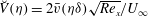
Figure 9 shows the behaviour of transmitted TS waves using the nonlinear base flows and the linearised calculations for the scattering of the TS waves. In this figure and for the subsequent calculation of the numerical transmission coefficient, we evaluate the transmission coefficient at a fixed
 $X$
location by determining the peak magnitude of the TS wave undergoing a distortion divided by the magnitude of the TS wave at the same
$X$
location by determining the peak magnitude of the TS wave undergoing a distortion divided by the magnitude of the TS wave at the same
 $X$
location over a flat plate. Therefore, as
$X$
location over a flat plate. Therefore, as
 $X\rightarrow \infty$
we expect to recover the theoretical transmission coefficient. In figure 9(a), within a range close to the distortions
$X\rightarrow \infty$
we expect to recover the theoretical transmission coefficient. In figure 9(a), within a range close to the distortions
 $X\in [-6,6]$
, it can be seen that the TS waves can indeed be stabilised (
$X\in [-6,6]$
, it can be seen that the TS waves can indeed be stabilised (
 ${\mathcal{T}}_{h}(X)<1$
) downstream of small-amplitude humps consistently with the theory. However, further downstream, as is shown in figure 9(b), this is not the case, and the overall influence of the hump is to destabilise the TS waves. Figure 9(c,d) demonstrates that, for the case of indentations, and for values of
${\mathcal{T}}_{h}(X)<1$
) downstream of small-amplitude humps consistently with the theory. However, further downstream, as is shown in figure 9(b), this is not the case, and the overall influence of the hump is to destabilise the TS waves. Figure 9(c,d) demonstrates that, for the case of indentations, and for values of
 ${\hat{h}}$
presented, the TS waves are always destabilised. For the current configurations, we therefore observe that humps and indentations have a similar destabilisation influence on TS waves. We further observe that, for the same
${\hat{h}}$
presented, the TS waves are always destabilised. For the current configurations, we therefore observe that humps and indentations have a similar destabilisation influence on TS waves. We further observe that, for the same
 ${\hat{h}}$
, the hump transmission coefficient,
${\hat{h}}$
, the hump transmission coefficient,
 ${\mathcal{T}}_{h}(\infty )$
, is greater than the indentation transmission coefficient,
${\mathcal{T}}_{h}(\infty )$
, is greater than the indentation transmission coefficient,
 ${\mathcal{T}}_{i}(\infty )$
(
${\mathcal{T}}_{i}(\infty )$
(
 $X\gg 1$
).
$X\gg 1$
).

Figure 10. Functions
 ${\mathcal{T}}_{\#}^{\ast }(X)/{\hat{h}}$
around humps and indentations (the notation ‘
${\mathcal{T}}_{\#}^{\ast }(X)/{\hat{h}}$
around humps and indentations (the notation ‘
 $\#$
’ denotes
$\#$
’ denotes
 $h$
or
$h$
or
 $i$
): (a)
$i$
): (a)
 ${\mathcal{T}}_{h}^{\ast }(X)/{\hat{h}}$
for
${\mathcal{T}}_{h}^{\ast }(X)/{\hat{h}}$
for
 $X\in [-6,6]$
; (b)
$X\in [-6,6]$
; (b)
 ${\mathcal{T}}_{h}^{\ast }(X)/{\hat{h}}$
for
${\mathcal{T}}_{h}^{\ast }(X)/{\hat{h}}$
for
 $X\in [6,35]$
; (c)
$X\in [6,35]$
; (c)
 ${\mathcal{T}}_{i}^{\ast }(X)/{\hat{h}}$
for
${\mathcal{T}}_{i}^{\ast }(X)/{\hat{h}}$
for
 $X\in [-6,6]$
; and (d)
$X\in [-6,6]$
; and (d)
 ${\mathcal{T}}_{i}^{\ast }(X)/{\hat{h}}$
for
${\mathcal{T}}_{i}^{\ast }(X)/{\hat{h}}$
for
 $X\in [6,35]$
. Here
$X\in [6,35]$
. Here
 $\mathit{Re}_{{\it\delta}_{\ast }}=1140.1$
and
$\mathit{Re}_{{\it\delta}_{\ast }}=1140.1$
and
 ${\mathcal{F}}=55.10$
;
${\mathcal{F}}=55.10$
;
 ${\hat{h}}=0.6$
(○), 0.8 (▫), 1 (♢), 1.2 (▵) and width
${\hat{h}}=0.6$
(○), 0.8 (▫), 1 (♢), 1.2 (▵) and width
 $\hat{d}=1$
.
$\hat{d}=1$
.
As already mentioned, we anticipate from (4.12) that
 $\mathscr{T}_{r}$
is dependent on
$\mathscr{T}_{r}$
is dependent on
 ${\hat{h}}$
for a fixed roughness profile
${\hat{h}}$
for a fixed roughness profile
 $\hat{F}(X)$
and so
$\hat{F}(X)$
and so
 ${\mathcal{T}}_{h}^{\ast }(X)/{\hat{h}}$
and
${\mathcal{T}}_{h}^{\ast }(X)/{\hat{h}}$
and
 ${\mathcal{T}}_{i}^{\ast }(X)/{\hat{h}}$
should collapse around the distortions. Therefore in figure 10 we consider the numerical transmission coefficient scaled by
${\mathcal{T}}_{i}^{\ast }(X)/{\hat{h}}$
should collapse around the distortions. Therefore in figure 10 we consider the numerical transmission coefficient scaled by
 ${\hat{h}}$
and observe an approximate collapse within a localised range
${\hat{h}}$
and observe an approximate collapse within a localised range
 $X\in [-1,1]$
. However, beyond this range, the distorted TS waves do not appear to collapse. This is due to the
$X\in [-1,1]$
. However, beyond this range, the distorted TS waves do not appear to collapse. This is due to the
 ${\it\varepsilon}^{1/4}$
scaling in (4.13). Clearly, owing to the distortion of the hump/indentation, the boundary layer is changed and, locally, the TS waves do not maintain similar growth and decay rates to those of TS waves in a flat-plate Blasius boundary layer. Wu & Hogg (Reference Wu and Hogg2006) put forward the model that the effect of a localised roughness element is to instantly ‘boost’ the amplitude of the TS waves. Nevertheless, this numerical study indicates that the amplification arises over quite a significant streamwise scale in the case of these relatively short streamwise scale distortions.
${\it\varepsilon}^{1/4}$
scaling in (4.13). Clearly, owing to the distortion of the hump/indentation, the boundary layer is changed and, locally, the TS waves do not maintain similar growth and decay rates to those of TS waves in a flat-plate Blasius boundary layer. Wu & Hogg (Reference Wu and Hogg2006) put forward the model that the effect of a localised roughness element is to instantly ‘boost’ the amplitude of the TS waves. Nevertheless, this numerical study indicates that the amplification arises over quite a significant streamwise scale in the case of these relatively short streamwise scale distortions.
In figure 11, we provide a comparison between a hump and an indentation with the same value of
 ${\hat{h}}=1$
(
${\hat{h}}=1$
(
 $h/{\it\delta}_{99}=3.9\,\%$
). From figure 11(a), it is clear that, when
$h/{\it\delta}_{99}=3.9\,\%$
). From figure 11(a), it is clear that, when
 $X\rightarrow \infty$
, the influence of humps on TS waves is greater than that of indentations. In addition, in figure 11(b), where we show the deviation of the transmission coefficient from a unit value and have reversed the sign in front of
$X\rightarrow \infty$
, the influence of humps on TS waves is greater than that of indentations. In addition, in figure 11(b), where we show the deviation of the transmission coefficient from a unit value and have reversed the sign in front of
 ${\mathcal{T}}_{i}^{\ast }(X)$
, we observe a similar qualitative behaviour. As a comparison, for a much smaller
${\mathcal{T}}_{i}^{\ast }(X)$
, we observe a similar qualitative behaviour. As a comparison, for a much smaller
 ${\hat{h}}=0.1$
(
${\hat{h}}=0.1$
(
 $h/{\it\delta}_{99}=0.39\,\%$
), the same conclusion can be drawn from figure 11(c,d) that the asymptotic theory does become valid at this smaller amplitude. Upstream of the hump and indentation, the profiles of
$h/{\it\delta}_{99}=0.39\,\%$
), the same conclusion can be drawn from figure 11(c,d) that the asymptotic theory does become valid at this smaller amplitude. Upstream of the hump and indentation, the profiles of
 ${\mathcal{T}}_{h}^{\ast }(X)/{\hat{h}}$
and
${\mathcal{T}}_{h}^{\ast }(X)/{\hat{h}}$
and
 $-{\mathcal{T}}_{i}^{\ast }(X)/{\hat{h}}$
have already collapsed very well. Although the hump and indentation subsequently demonstrate different magnitudes of destabilisation of the TS waves downstream of the hump and indentation, the overall pattern is much more similar than for the
$-{\mathcal{T}}_{i}^{\ast }(X)/{\hat{h}}$
have already collapsed very well. Although the hump and indentation subsequently demonstrate different magnitudes of destabilisation of the TS waves downstream of the hump and indentation, the overall pattern is much more similar than for the
 ${\hat{h}}=1$
case. Clearly this supports the trend that, as
${\hat{h}}=1$
case. Clearly this supports the trend that, as
 ${\hat{h}}\rightarrow 0$
,
${\hat{h}}\rightarrow 0$
,
 ${\mathcal{T}}_{h}^{\ast }(X)/{\hat{h}}$
and
${\mathcal{T}}_{h}^{\ast }(X)/{\hat{h}}$
and
 $-{\mathcal{T}}_{i}^{\ast }(X)/{\hat{h}}$
will indeed collapse and the numerical results recover the linear theory.
$-{\mathcal{T}}_{i}^{\ast }(X)/{\hat{h}}$
will indeed collapse and the numerical results recover the linear theory.
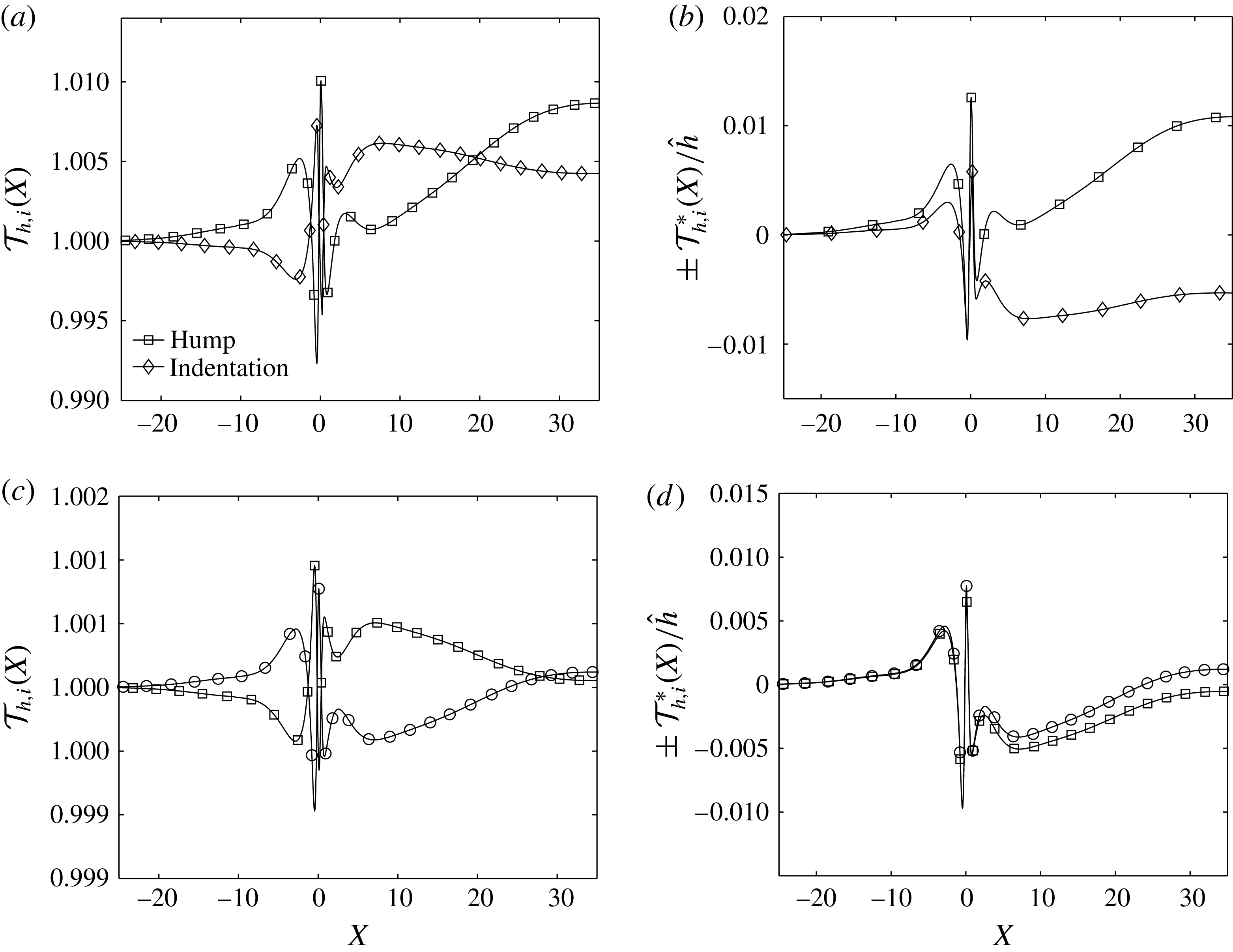
Figure 11. Comparisons of
 ${\mathcal{T}}_{h,i}(X)$
and
${\mathcal{T}}_{h,i}(X)$
and
 ${\mathcal{T}}_{h,i}^{\ast }(X)/{\hat{h}}$
: (a)
${\mathcal{T}}_{h,i}^{\ast }(X)/{\hat{h}}$
: (a)
 ${\mathcal{T}}_{h,i}(X)$
for
${\mathcal{T}}_{h,i}(X)$
for
 ${\hat{h}}=1$
; (b)
${\hat{h}}=1$
; (b)
 ${\mathcal{T}}_{h}^{\ast }(X)/{\hat{h}}$
and
${\mathcal{T}}_{h}^{\ast }(X)/{\hat{h}}$
and
 $-{\mathcal{T}}_{i}^{\ast }(X)/{\hat{h}}$
for
$-{\mathcal{T}}_{i}^{\ast }(X)/{\hat{h}}$
for
 ${\hat{h}}=1$
; (c)
${\hat{h}}=1$
; (c)
 ${\mathcal{T}}_{h,i}(X)$
for
${\mathcal{T}}_{h,i}(X)$
for
 ${\hat{h}}=0.1$
; and (d)
${\hat{h}}=0.1$
; and (d)
 ${\mathcal{T}}_{h}^{\ast }(X)/{\hat{h}}$
and
${\mathcal{T}}_{h}^{\ast }(X)/{\hat{h}}$
and
 $-{\mathcal{T}}_{i}^{\ast }(X)/{\hat{h}}$
for
$-{\mathcal{T}}_{i}^{\ast }(X)/{\hat{h}}$
for
 ${\hat{h}}=0.1$
. The roughness elements are located at
${\hat{h}}=0.1$
. The roughness elements are located at
 $\mathit{Re}_{{\it\delta}_{\ast }}=1140.1$
. Here
$\mathit{Re}_{{\it\delta}_{\ast }}=1140.1$
. Here
 ${\mathcal{F}}=55.10$
and the width
${\mathcal{F}}=55.10$
and the width
 $\hat{d}=1$
.
$\hat{d}=1$
.
4.3.1 Effect of height and width of distortion on the transmission coefficient
For the range
 $0.05<{\hat{h}}<1.4$
(
$0.05<{\hat{h}}<1.4$
(
 $0.4\,\%<h/{\it\delta}_{99}<5.5\,\%$
) currently considered with
$0.4\,\%<h/{\it\delta}_{99}<5.5\,\%$
) currently considered with
 $\hat{d}=1$
, we have only observed a transmission coefficient of maximum
$\hat{d}=1$
, we have only observed a transmission coefficient of maximum
 $2\,\%$
. For this numerical study we have fixed our value of Reynolds number to
$2\,\%$
. For this numerical study we have fixed our value of Reynolds number to
 $\mathit{Re}_{x_{c}}=440\,000$
and so the TS wave grows spatially with a growth rate of
$\mathit{Re}_{x_{c}}=440\,000$
and so the TS wave grows spatially with a growth rate of
 ${\it\alpha}_{i}=-0.011$
at
${\it\alpha}_{i}=-0.011$
at
 $\mathit{Re}_{x_{c}}=878\,036$
. If we assume that transition arises downstream of the distortion when the TS wave magnitude
$\mathit{Re}_{x_{c}}=878\,036$
. If we assume that transition arises downstream of the distortion when the TS wave magnitude
 $A_{0}$
has grown approximately
$A_{0}$
has grown approximately
 $\ln (A_{T}/A_{0})=3$
, then the transition would arise at
$\ln (A_{T}/A_{0})=3$
, then the transition would arise at
 $X=130$
(approximately
$X=130$
(approximately
 $130{\it\delta}_{99}$
) downstream of the initial position of the TS (and where we place the distortion). Under this set of assumptions, if
$130{\it\delta}_{99}$
) downstream of the initial position of the TS (and where we place the distortion). Under this set of assumptions, if
 ${\mathcal{T}}_{\#}^{\ast }(\infty )$
has values
${\mathcal{T}}_{\#}^{\ast }(\infty )$
has values
 $1\,\%$
,
$1\,\%$
,
 $10\,\%$
and
$10\,\%$
and
 $100\,\%$
, these will lead to a change of
$100\,\%$
, these will lead to a change of
 $0.36\,\%$
,
$0.36\,\%$
,
 $3.37\,\%$
and
$3.37\,\%$
and
 $24.0\,\%$
of the distance from the distortion to the point of transition. Clearly, from a practical point of view, we would like to understand what features lead to a larger transmission coefficient.
$24.0\,\%$
of the distance from the distortion to the point of transition. Clearly, from a practical point of view, we would like to understand what features lead to a larger transmission coefficient.
The main geometric features which could lead to a change in transmission coefficient are a change in
 ${\hat{h}}$
and
${\hat{h}}$
and
 $\hat{d}$
. A non-exhaustive investigation can be summarised in the data in figure 12. In this figure we show the variation of the transmission coefficient as a function of
$\hat{d}$
. A non-exhaustive investigation can be summarised in the data in figure 12. In this figure we show the variation of the transmission coefficient as a function of
 ${\hat{h}}$
at
${\hat{h}}$
at
 $\hat{d}=1$
as well as reduced set of data points for
$\hat{d}=1$
as well as reduced set of data points for
 $\hat{d}={\it\lambda}_{TS},{\it\lambda}_{TS}/2$
and
$\hat{d}={\it\lambda}_{TS},{\it\lambda}_{TS}/2$
and
 ${\it\lambda}_{TS}/3$
.
${\it\lambda}_{TS}/3$
.
If we assume that there exists a relation between
 ${\mathcal{T}}_{\#}(\infty )$
,
${\mathcal{T}}_{\#}(\infty )$
,
 $\hat{F}(0)$
and
$\hat{F}(0)$
and
 ${\hat{h}}$
of the form
${\hat{h}}$
of the form
 $$\begin{eqnarray}{\mathcal{T}}_{\#}(\infty )=1+{\it\Lambda}{\hat{h}}^{{\it\alpha}}\hat{F}(0),\end{eqnarray}$$
where
 ${\it\Lambda}$
is a constant, an empirical fit to the exponent
${\it\Lambda}$
is a constant, an empirical fit to the exponent
 ${\it\alpha}$
can be determined from the log–log plotting of the data in figure 12. We observe that, for very small values of
${\it\alpha}$
can be determined from the log–log plotting of the data in figure 12. We observe that, for very small values of
 ${\hat{h}}$
, where we observed that the transmission coefficient did tend to follow the linear theory, a value of approximately
${\hat{h}}$
, where we observed that the transmission coefficient did tend to follow the linear theory, a value of approximately
 ${\it\alpha}=1.5$
is observed. When we continue to increase
${\it\alpha}=1.5$
is observed. When we continue to increase
 ${\hat{h}}$
so that the flow around the hump and indentation are no longer similar (
${\hat{h}}$
so that the flow around the hump and indentation are no longer similar (
 $0.1<{\hat{h}}<1.4$
), but the flow remains attached, we observe a potential fit of
$0.1<{\hat{h}}<1.4$
), but the flow remains attached, we observe a potential fit of
 ${\it\alpha}\approx 2$
. For even larger values of
${\it\alpha}\approx 2$
. For even larger values of
 ${\hat{h}}$
(
${\hat{h}}$
(
 $h/{\it\delta}_{99}=7.2\,\%$
), the flow becomes detached, and at a value of
$h/{\it\delta}_{99}=7.2\,\%$
), the flow becomes detached, and at a value of
 ${\hat{h}}=5$
(
${\hat{h}}=5$
(
 $h/{\it\delta}_{99}=20\,\%$
) we observe a transmission coefficient of
$h/{\it\delta}_{99}=20\,\%$
) we observe a transmission coefficient of
 $350\,\%$
for the hump. For distortions of
$350\,\%$
for the hump. For distortions of
 $\hat{d}=1$
, we clearly only see significant transmission coefficients when the height has become sufficiently large and in this case the flow has separated from the distortion. Further, when
$\hat{d}=1$
, we clearly only see significant transmission coefficients when the height has become sufficiently large and in this case the flow has separated from the distortion. Further, when
 ${\mathcal{T}}_{h}^{\ast }(X)$
and
${\mathcal{T}}_{h}^{\ast }(X)$
and
 ${\mathcal{T}}_{i}^{\ast }(X)$
are rescaled by
${\mathcal{T}}_{i}^{\ast }(X)$
are rescaled by
 ${\hat{h}}^{2.11}$
and
${\hat{h}}^{2.11}$
and
 ${\hat{h}}^{1.85}$
, respectively, we observe an approximate collapse further downstream for both
${\hat{h}}^{1.85}$
, respectively, we observe an approximate collapse further downstream for both
 ${\mathcal{T}}_{h}^{\ast }(X)/{\hat{h}}^{2.11}$
and
${\mathcal{T}}_{h}^{\ast }(X)/{\hat{h}}^{2.11}$
and
 ${\mathcal{T}}_{i}^{\ast }(X)/{\hat{h}}^{1.85}$
in figure 13.
${\mathcal{T}}_{i}^{\ast }(X)/{\hat{h}}^{1.85}$
in figure 13.

Figure 12. Transmission coefficient
 ${\mathcal{T}}_{\#}$
(the notation ‘
${\mathcal{T}}_{\#}$
(the notation ‘
 $\#$
’ denotes
$\#$
’ denotes
 $h$
or
$h$
or
 $i$
): (a) for humps; and (b) for indentations. Symbols denotes cases where the flow is attached (○) and cases where the flow is separated (▫) when
$i$
): (a) for humps; and (b) for indentations. Symbols denotes cases where the flow is attached (○) and cases where the flow is separated (▫) when
 $\hat{d}=1$
. Other symbols denote attached flow when
$\hat{d}=1$
. Other symbols denote attached flow when
 $\hat{d}={\it\lambda}_{TS}/3$
(♢),
$\hat{d}={\it\lambda}_{TS}/3$
(♢),
 $\hat{d}={\it\lambda}_{TS}/2$
(▵) and
$\hat{d}={\it\lambda}_{TS}/2$
(▵) and
 $\hat{d}={\it\lambda}_{TS}$
(▿).
$\hat{d}={\it\lambda}_{TS}$
(▿).

Figure 13. Functions
 ${\mathcal{T}}_{\#}^{\ast }(X)/{\hat{h}}$
around humps and indentations (the notation ‘
${\mathcal{T}}_{\#}^{\ast }(X)/{\hat{h}}$
around humps and indentations (the notation ‘
 $\#$
’ denotes
$\#$
’ denotes
 $h$
or
$h$
or
 $i$
): (a)
$i$
): (a)
 ${\mathcal{T}}_{h}^{\ast }(X)/{\hat{h}}^{2.11}$
for
${\mathcal{T}}_{h}^{\ast }(X)/{\hat{h}}^{2.11}$
for
 $X\in [6,35]$
; and (b)
$X\in [6,35]$
; and (b)
 ${\mathcal{T}}_{i}^{\ast }(X)/{\hat{h}}^{1.85}$
for
${\mathcal{T}}_{i}^{\ast }(X)/{\hat{h}}^{1.85}$
for
 $X\in [6,35]$
. Here
$X\in [6,35]$
. Here
 $\mathit{Re}_{{\it\delta}_{\ast }}=1140.1$
and
$\mathit{Re}_{{\it\delta}_{\ast }}=1140.1$
and
 ${\mathcal{F}}=55.10$
;
${\mathcal{F}}=55.10$
;
 ${\hat{h}}=0.6$
(○), 0.8 (▫), 1 (♢), 1.2 (▵) and width
${\hat{h}}=0.6$
(○), 0.8 (▫), 1 (♢), 1.2 (▵) and width
 $\hat{d}=1$
.
$\hat{d}=1$
.
However, when the distortion has a width that is comparable with the TS wavelength, large transmission coefficients are also possible. This factor is encapsulated by the
 $\hat{F}(0)$
term in (4.12) and (4.14), which we recall represents the Fourier transform of the roughness element. The data for
$\hat{F}(0)$
term in (4.12) and (4.14), which we recall represents the Fourier transform of the roughness element. The data for
 $\hat{d}={\it\lambda}_{TS},~{\it\lambda}_{TS}/2,~{\it\lambda}_{TS}/3$
as opposed to the values for when
$\hat{d}={\it\lambda}_{TS},~{\it\lambda}_{TS}/2,~{\it\lambda}_{TS}/3$
as opposed to the values for when
 $\hat{d}=1={\it\lambda}_{TS}/11.3$
lead to far larger transmission coefficients, nearly an order of magnitude higher. We also observe that, in the range of data considered, the slope of
$\hat{d}=1={\it\lambda}_{TS}/11.3$
lead to far larger transmission coefficients, nearly an order of magnitude higher. We also observe that, in the range of data considered, the slope of
 ${\it\alpha}\approx 2$
seems to remain. If the analysis of Wu & Hogg (Reference Wu and Hogg2006) is extended to include the weak nonlinearity of the base flow distortion, then
${\it\alpha}\approx 2$
seems to remain. If the analysis of Wu & Hogg (Reference Wu and Hogg2006) is extended to include the weak nonlinearity of the base flow distortion, then
 $$\begin{eqnarray}\mathscr{T}_{r}=1+{\it\Lambda}_{1}{\it\varepsilon}^{1/4}{\hat{h}}+{\it\Lambda}_{2}{\hat{h}}^{2},\end{eqnarray}$$
where
 ${\it\Lambda}_{2}\sim \mathit{O}(1)$
. The result indicates that the linear approximation requires a more stringent condition
${\it\Lambda}_{2}\sim \mathit{O}(1)$
. The result indicates that the linear approximation requires a more stringent condition
 ${\hat{h}}\ll {\it\varepsilon}^{1/4}$
rather than
${\hat{h}}\ll {\it\varepsilon}^{1/4}$
rather than
 ${\hat{h}}\ll 1$
. Therefore, when
${\hat{h}}\ll 1$
. Therefore, when
 ${\it\varepsilon}^{1/4}\ll {\hat{h}}\ll 1$
, there is a degeneracy of the linear mechanism, where the transmission coefficient can be seen to behave primarily as a quadratic function of
${\it\varepsilon}^{1/4}\ll {\hat{h}}\ll 1$
, there is a degeneracy of the linear mechanism, where the transmission coefficient can be seen to behave primarily as a quadratic function of
 ${\hat{h}}$
.
${\hat{h}}$
.
4.3.2 Effect of multiple isolated roughness elements on the TS transmission coefficient
Individually, when
 $\hat{d}=1$
we have observed that the effect of a single isolated small-scale localised distortion on the TS waves is small. Therefore, we consider the effect of multiple isolated roughness elements. Since multiple isolated humps have a similar destabilisation effect on the TS waves as multiple isolated indentations, we consider only the cases of three isolated humps located at
$\hat{d}=1$
we have observed that the effect of a single isolated small-scale localised distortion on the TS waves is small. Therefore, we consider the effect of multiple isolated roughness elements. Since multiple isolated humps have a similar destabilisation effect on the TS waves as multiple isolated indentations, we consider only the cases of three isolated humps located at
 $\mathit{Re}_{{\it\delta}_{\ast }}=1140.17,~1166.07$
and
$\mathit{Re}_{{\it\delta}_{\ast }}=1140.17,~1166.07$
and
 $1191.40$
, as is illustrated in figure 14. The three humps are equally spaced and the distance between two adjacent humps is equal to six times the upper-deck scale defined at
$1191.40$
, as is illustrated in figure 14. The three humps are equally spaced and the distance between two adjacent humps is equal to six times the upper-deck scale defined at
 $\mathit{Re}_{{\it\delta}_{\ast }}=1140.17$
or approximately
$\mathit{Re}_{{\it\delta}_{\ast }}=1140.17$
or approximately
 $6{\it\delta}_{99}$
. The width and height of these three humps are kept the same, which are also defined by the local scales of the first hump located at
$6{\it\delta}_{99}$
. The width and height of these three humps are kept the same, which are also defined by the local scales of the first hump located at
 $\mathit{Re}_{{\it\delta}_{\ast }}=1140.17$
. For the first hump, the width scale
$\mathit{Re}_{{\it\delta}_{\ast }}=1140.17$
. For the first hump, the width scale
 $\hat{d}$
is fixed equal to 1 and the height scale considered includes
$\hat{d}$
is fixed equal to 1 and the height scale considered includes
 ${\hat{h}}=0.6$
, 0.8, 1.0, 1.2 and 1.4. For all cases, there is no separated flow; and the base flow, shear stress and pressure gradients were similar to the isolated cases and are not shown.
${\hat{h}}=0.6$
, 0.8, 1.0, 1.2 and 1.4. For all cases, there is no separated flow; and the base flow, shear stress and pressure gradients were similar to the isolated cases and are not shown.
The base flow for
 ${\hat{h}}=1.4$
is illustrated in figure 14. Figure 15 shows the profiles of the numerical transmission coefficient for the series of three humps. From figure 15(a), we can observe that higher
${\hat{h}}=1.4$
is illustrated in figure 14. Figure 15 shows the profiles of the numerical transmission coefficient for the series of three humps. From figure 15(a), we can observe that higher
 ${\hat{h}}$
values give rise to a relatively large amplification of the TS waves. When
${\hat{h}}$
values give rise to a relatively large amplification of the TS waves. When
 ${\hat{h}}=1.4$
(
${\hat{h}}=1.4$
(
 $h/{\it\delta}_{99}=5.5\,\%$
), the amplification of the corresponding TS wave is approximately 10 %. In figure 15(b), we provide a comparison between multiple humps and a single hump when
$h/{\it\delta}_{99}=5.5\,\%$
), the amplification of the corresponding TS wave is approximately 10 %. In figure 15(b), we provide a comparison between multiple humps and a single hump when
 ${\hat{h}}=0.8$
and we observe that the amplification of the TS wave by three humps is very close to three times that by a single hump. For the current configuration, there exists a linear relation between the amplification and number of isolated humps. The effect of multiple humps would theoretically be expected to have a multiplicative influence. However, since each hump has a small transmission coefficient, a linearisation of a multiplicative transmission coefficient gives a linear amplification as observed here. We recall from figure 9(a) that for
${\hat{h}}=0.8$
and we observe that the amplification of the TS wave by three humps is very close to three times that by a single hump. For the current configuration, there exists a linear relation between the amplification and number of isolated humps. The effect of multiple humps would theoretically be expected to have a multiplicative influence. However, since each hump has a small transmission coefficient, a linearisation of a multiplicative transmission coefficient gives a linear amplification as observed here. We recall from figure 9(a) that for
 ${\hat{h}}=0.6$
at a location of
${\hat{h}}=0.6$
at a location of
 $X=6$
there exists a small region of stabilisation of the TS waves. However, in the case of multiple humps, spaced by six units, the overall effect is still to destabilise the TS waves.
$X=6$
there exists a small region of stabilisation of the TS waves. However, in the case of multiple humps, spaced by six units, the overall effect is still to destabilise the TS waves.

Figure 14. Base flow for
 ${\hat{h}}=1.4$
: (a) horizontal velocity; and (b) vertical velocity.
${\hat{h}}=1.4$
: (a) horizontal velocity; and (b) vertical velocity.

Figure 15. Profiles of
 ${\mathcal{T}}_{mh}^{\ast }(X)$
and
${\mathcal{T}}_{mh}^{\ast }(X)$
and
 ${\mathcal{T}}_{\#}^{\ast }(X)/{\hat{h}}$
: (a) profiles of
${\mathcal{T}}_{\#}^{\ast }(X)/{\hat{h}}$
: (a) profiles of
 ${\it\tau}_{mh}^{\ast }(X)$
(height scales
${\it\tau}_{mh}^{\ast }(X)$
(height scales
 ${\hat{h}}=0.6$
(○), 0.8 (▫), 1.0 (♢), 1.2 (▵), 1.4 (▿)); and (b) profiles of
${\hat{h}}=0.6$
(○), 0.8 (▫), 1.0 (♢), 1.2 (▵), 1.4 (▿)); and (b) profiles of
 ${\it\tau}_{mh}^{\ast }(X)/{\hat{h}}$
for multiple humps (○) and a single hump (▫). The width
${\it\tau}_{mh}^{\ast }(X)/{\hat{h}}$
for multiple humps (○) and a single hump (▫). The width
 $\hat{d}=1$
. The frequency
$\hat{d}=1$
. The frequency
 ${\mathcal{F}}=55.10$
. Notation
${\mathcal{F}}=55.10$
. Notation
 $\#$
denotes the single-hump symbol ‘
$\#$
denotes the single-hump symbol ‘
 $h$
’ or the multiple-hump symbol ‘
$h$
’ or the multiple-hump symbol ‘
 $mh$
’.
$mh$
’.
5 Conclusion
In this paper, the spectral element discretisation was employed to numerically analyse the behaviour of the TS waves when the base flow is distorted by a small-scale localised distortion. The base flows were obtained using the fully nonlinear Navier–Stokes equations and the TS wave amplifications was simulated using the linearised Navier–Stokes equations.
For the small-amplitude localised wall distortions considered, humps and indentations both have destabilising effects rather than having opposite effects as expected on the basis of linearity. This indicates that the nonlinearity effect is appreciable despite the relatively small height/depth of humps/indentations. The result is broadly consistent with the degeneracy of the leading-order linear term of the asymptotic analysis.
Notably, for the regime investigated,
 $0.05<{\hat{h}}<1.4$
(
$0.05<{\hat{h}}<1.4$
(
 $0.2\,\%<h/{\it\delta}_{99}<5.5\,\%$
) at
$0.2\,\%<h/{\it\delta}_{99}<5.5\,\%$
) at
 $\mathit{Re}_{{\it\delta}_{\ast }}=1140.17$
or
$\mathit{Re}_{{\it\delta}_{\ast }}=1140.17$
or
 $\mathit{Re}_{x_{c}}=440\,000$
, we observe that, when the transmission coefficient is evaluated downstream of the distortion, both humps and indentations have a destabilising effect on the TS wave, in contrast to the asymptotic theory for smoother distortions, where only indentations were observed to be destabilising in the vicinity of the distortion. The localised distortions considered in this study lead to a significant deviation of the flow from the Blasius flat-plate profile, which is consistent with the deviation of the numerical results from the linearised asymptotic theory. For the parameters studied, an isolated distortion leads to a relatively weak, of the order of 1–2 %, amplification of the TS wave when
$\mathit{Re}_{x_{c}}=440\,000$
, we observe that, when the transmission coefficient is evaluated downstream of the distortion, both humps and indentations have a destabilising effect on the TS wave, in contrast to the asymptotic theory for smoother distortions, where only indentations were observed to be destabilising in the vicinity of the distortion. The localised distortions considered in this study lead to a significant deviation of the flow from the Blasius flat-plate profile, which is consistent with the deviation of the numerical results from the linearised asymptotic theory. For the parameters studied, an isolated distortion leads to a relatively weak, of the order of 1–2 %, amplification of the TS wave when
 $\hat{d}=1$
. Increasing the height of the distortion so that the flow locally separates can lead to a much larger transmission coefficient of up to
$\hat{d}=1$
. Increasing the height of the distortion so that the flow locally separates can lead to a much larger transmission coefficient of up to
 $350\,\%$
in the case of a hump of size
$350\,\%$
in the case of a hump of size
 ${\hat{h}}=5$
(corresponding to
${\hat{h}}=5$
(corresponding to
 $h/{\it\delta}_{99}=20\,\%$
). In addition, if the hump width is increased to be comparable with the TS wavelength, an increase of nearly one order of magnitude was observed for a fixed hump height.
$h/{\it\delta}_{99}=20\,\%$
). In addition, if the hump width is increased to be comparable with the TS wavelength, an increase of nearly one order of magnitude was observed for a fixed hump height.
Finally the introduction of multiple humps when
 $\hat{d}=1$
(with a separation of six hump widths) is observed to have an additive effect, allowing the small distortions to obtain more significant amplifications.
$\hat{d}=1$
(with a separation of six hump widths) is observed to have an additive effect, allowing the small distortions to obtain more significant amplifications.
Acknowledgements
This research was performed in the Laminar Flow Control Centre (LFC-UK) at Imperial College London. The Centre is supported by EPSRC, Airbus Global Innovations under grant EP/I037946/1. S.J.S. would like to acknowledge support under a Royal Academy of Engineering Research chair. We would also like to acknowledge the helpful input of Gianmarco Mengaldo.
Appendix A. Interaction described by the triple-deck theory
The asymptotic expansions in each deck are given as follows.
-
(1) Upper deck:
(A 1)The equations are $$\begin{eqnarray}\left.\begin{array}{@{}l@{}}u=1+{\it\varepsilon}^{1/2}u_{1}^{\ast }(X,Y^{\ast })+\cdots \!,\\ v={\it\varepsilon}^{1/2}v_{1}^{\ast }(X,Y^{\ast })+\cdots \!,\\ p={\it\varepsilon}^{1/2}p_{1}^{\ast }(X,Y^{\ast })+\cdots \!.\end{array}\right\}\end{eqnarray}$$
(A 2a )
$$\begin{eqnarray}\displaystyle & \displaystyle \frac{\partial u_{1}^{\ast }}{\partial X}+\frac{\partial v_{1}^{\ast }}{\partial Y^{\ast }}=0, & \displaystyle\end{eqnarray}$$
(A 2b )
$$\begin{eqnarray}\displaystyle & \displaystyle \frac{\partial u_{1}^{\ast }}{\partial X}=-\frac{\partial p_{1}^{\ast }}{\partial X}, & \displaystyle\end{eqnarray}$$
(A 2c )
$$\begin{eqnarray}\displaystyle & \displaystyle \frac{\partial V_{1}^{\ast }}{\partial X}=-\frac{\partial p_{1}^{\ast }}{\partial Y^{\ast }}. & \displaystyle\end{eqnarray}$$
$$\begin{eqnarray}\left.\begin{array}{@{}l@{}}u=1+{\it\varepsilon}^{1/2}u_{1}^{\ast }(X,Y^{\ast })+\cdots \!,\\ v={\it\varepsilon}^{1/2}v_{1}^{\ast }(X,Y^{\ast })+\cdots \!,\\ p={\it\varepsilon}^{1/2}p_{1}^{\ast }(X,Y^{\ast })+\cdots \!.\end{array}\right\}\end{eqnarray}$$
(A 2a )
$$\begin{eqnarray}\displaystyle & \displaystyle \frac{\partial u_{1}^{\ast }}{\partial X}+\frac{\partial v_{1}^{\ast }}{\partial Y^{\ast }}=0, & \displaystyle\end{eqnarray}$$
(A 2b )
$$\begin{eqnarray}\displaystyle & \displaystyle \frac{\partial u_{1}^{\ast }}{\partial X}=-\frac{\partial p_{1}^{\ast }}{\partial X}, & \displaystyle\end{eqnarray}$$
(A 2c )
$$\begin{eqnarray}\displaystyle & \displaystyle \frac{\partial V_{1}^{\ast }}{\partial X}=-\frac{\partial p_{1}^{\ast }}{\partial Y^{\ast }}. & \displaystyle\end{eqnarray}$$
-
(2) Main deck:
(A 3)The equations are
$$\begin{eqnarray}\left.\begin{array}{@{}l@{}}u=U_{B}+{\it\varepsilon}^{1/4}u_{1}(X,Y^{\ast })+\cdots \!,\\ v={\it\varepsilon}^{1/2}v_{1}(X,Y^{\ast })+\cdots \!,\\ p={\it\varepsilon}^{1/2}p_{1}(X,Y^{\ast })+\cdots \!.\end{array}\right\}\end{eqnarray}$$
The solution in the main deck is(A 4a )
$$\begin{eqnarray}\displaystyle & \displaystyle \frac{\partial u_{1}}{\partial X}+\frac{\partial v_{1}}{\partial Y}=0, & \displaystyle\end{eqnarray}$$
(A 4b )
$$\begin{eqnarray}\displaystyle & \displaystyle U_{B}\frac{\partial u_{1}}{\partial X}+u_{1}\frac{\partial U_{0}}{\partial Y}=0, & \displaystyle\end{eqnarray}$$
(A 4c )
$$\begin{eqnarray}\displaystyle & \displaystyle \frac{\partial P_{1}}{\partial Y}=0. & \displaystyle\end{eqnarray}$$
where the function(A 5a )
$$\begin{eqnarray}\displaystyle & \displaystyle u_{1}=A(X)U_{B}^{\prime }(Y)\quad \text{with }U_{B}^{\prime }(Y)=\frac{\text{d}U_{B}}{\text{d}Y}, & \displaystyle\end{eqnarray}$$
(A 5b )
$$\begin{eqnarray}\displaystyle & \displaystyle v_{1}=-A(X)U_{B}(Y)\quad \text{with }A^{\prime }(X)=\frac{\text{d}A}{\text{d}X}, & \displaystyle\end{eqnarray}$$
$A(X)$
is called a displacement function, which can be determined such that
$A\rightarrow 0$
as
$X\rightarrow -\infty$
.
-
(3) Lower deck:
(A 6)The equations are
$$\begin{eqnarray}\left.\begin{array}{@{}l@{}}u={\it\varepsilon}^{1/4}\hat{u} _{1}(X,{\hat{Y}})+\cdots \!,\\ v={\it\varepsilon}^{3/4}\hat{v}_{1}(X,{\hat{Y}})+\cdots \!,\\ p={\it\varepsilon}^{1/2}\hat{p}_{1}(X,{\hat{Y}})+\cdots \!.\end{array}\right\}\end{eqnarray}$$
(A 7a )
$$\begin{eqnarray}\displaystyle & \displaystyle \frac{\partial \hat{u} _{1}}{\partial X}+\displaystyle \frac{\partial \hat{v}_{1}}{\partial {\hat{Y}}}=0, & \displaystyle\end{eqnarray}$$
(A 7b )
$$\begin{eqnarray}\displaystyle & \displaystyle \hat{u} _{1}\frac{\partial \hat{u} _{1}}{\partial X}+\hat{v}_{1}\frac{\partial \hat{u} _{1}}{\partial {\hat{Y}}}=\displaystyle -\frac{\partial \hat{p}_{1}}{\partial X}+\frac{\partial ^{2}\hat{u} _{1}}{\partial {\hat{Y}}^{2}}, & \displaystyle\end{eqnarray}$$
(A 7c )
$$\begin{eqnarray}\displaystyle & \displaystyle \frac{\partial \hat{p}_{1}}{\partial {\hat{Y}}}=0. & \displaystyle\end{eqnarray}$$


Asymptotically, to order
 ${\it\varepsilon}^{1/4}$
, we obtain
${\it\varepsilon}^{1/4}$
, we obtain
 $$\begin{eqnarray}\lim _{{\hat{Y}}\rightarrow \infty }(\hat{u} _{1}-{\it\lambda}{\hat{Y}})={\it\lambda}A(X).\end{eqnarray}$$
To order
 ${\it\varepsilon}^{1/2}$
, we have
${\it\varepsilon}^{1/2}$
, we have
 $$\begin{eqnarray}v_{1}^{\ast }(X,0)=\lim _{Y\rightarrow 0}v_{1}(X,Y).\end{eqnarray}$$
Considering (A 3) amd
 $U_{B}(\infty )=1$
, we have
$U_{B}(\infty )=1$
, we have
 $$\begin{eqnarray}v_{1}^{\ast }(X,0)=\frac{\text{d}A}{\text{d}X}.\end{eqnarray}$$
For pressure
 $p$
, to order
$p$
, to order
 ${\it\varepsilon}^{1/2}$
, the asymptotic matching gives
${\it\varepsilon}^{1/2}$
, the asymptotic matching gives
 $$\begin{eqnarray}\displaystyle & \displaystyle p_{1}(X,0)=\lim _{{\hat{Y}}\rightarrow 0}\hat{p}(X,{\hat{Y}}), & \displaystyle\end{eqnarray}$$
 $$\begin{eqnarray}\displaystyle & \displaystyle p_{1}^{\ast }(X,0)=\lim _{Y\rightarrow 0}p_{1}(X,Y). & \displaystyle\end{eqnarray}$$
 $\displaystyle \frac{\partial p_{1}}{\partial Y}=0$
and
$\displaystyle \frac{\partial p_{1}}{\partial Y}=0$
and
 $\displaystyle \frac{\partial \hat{p}_{1}}{\partial {\hat{Y}}}=0$
, we have
$\displaystyle \frac{\partial \hat{p}_{1}}{\partial {\hat{Y}}}=0$
, we have  $$\begin{eqnarray}p_{1}^{\ast }(X,0)=p_{1}(X)=\hat{p}_{1}(X).\end{eqnarray}$$
For subsonic main stream flow,
 $$\begin{eqnarray}A^{\prime \prime }(X)=-\frac{1}{{\rm\pi}}\int _{-\infty }^{\infty }\frac{\hat{p}^{\prime }({\it\xi})}{X-{\it\xi}}\,\text{d}{\it\xi}.\end{eqnarray}$$
Appendix B. Definitions of parameters in (4.9)
 $$\begin{eqnarray}\displaystyle & \displaystyle {\it\alpha}=\left\{\begin{array}{@{}lr@{}}\displaystyle \int _{0}^{\infty }\frac{s^{2}(3^{1/2}s^{4/3}-2)\exp (-{\it\theta}st)\,\text{d}s}{1-3^{1/2}s^{4/3}+s^{8/3}} & (t>0),\\ 2\displaystyle \int _{0}^{\infty }\frac{s^{2}\exp ({\it\theta}st)\,\text{d}s}{1+s^{8/3}} & (t<0),\end{array}\right. & \displaystyle\end{eqnarray}$$
 $$\begin{eqnarray}\displaystyle & \displaystyle {\it\beta}=\left\{\begin{array}{@{}lr@{}}\displaystyle \int _{0}^{\infty }\frac{s^{5/3}(3^{1/2}s^{4/3}-1)\exp (-{\it\theta}st)\,\text{d}s}{1-3^{1/2}s^{4/3}+s^{8/3}} & (t>0),\\ 2\displaystyle \int _{0}^{\infty }\frac{s^{5/3}\exp ({\it\theta}st)\,\text{d}s}{1+s^{8/3}} & (t<0).\end{array}\right. & \displaystyle\end{eqnarray}$$
Appendix C. Definitions of parameters in (41.3)
The functions
 $K(\cdot ,\!\cdot )$
and
$K(\cdot ,\!\cdot )$
and
 ${\it\Delta}(\cdot )$
respectively are defined by
${\it\Delta}(\cdot )$
respectively are defined by
 $$\begin{eqnarray}K({\it\eta},{\it\eta}_{0})={\rm\pi}\frac{\text{Ai}^{\prime }({\it\eta}_{0})\text{Gi}({\it\eta})-\text{Gi}^{\prime }({\it\eta}_{0})\text{Ai}({\it\eta})}{\text{Ai}^{\prime }({\it\eta})},\end{eqnarray}$$
and
 $$\begin{eqnarray}{\it\Delta}(k)=\int _{{\it\eta}_{0}}^{\infty }\text{Ai}({\it\zeta})\,\text{d}{\it\zeta}+\text{i}{\it\lambda}(\text{i}k{\it\lambda})^{2/3}\text{Ai}^{\prime }({\it\eta}_{0})\frac{\bar{k}}{k^{3}},\end{eqnarray}$$
where
 $\text{Gi}$
and
$\text{Gi}$
and
 $\text{Gi}^{\prime }$
are defined in Abramowitz & Stegun (Reference Abramowitz and Stegun1964, p. 449), and where
$\text{Gi}^{\prime }$
are defined in Abramowitz & Stegun (Reference Abramowitz and Stegun1964, p. 449), and where
 $\bar{k}=(1-M^{2})^{1/2}|k|$
(
$\bar{k}=(1-M^{2})^{1/2}|k|$
(
 $M$
is the Mach number and
$M$
is the Mach number and
 $M<1$
for the subsonic flow). In the theory, the TS wave has a wavenumber
$M<1$
for the subsonic flow). In the theory, the TS wave has a wavenumber
 ${\it\alpha}$
and the mean-flow distortion has a continuous Fourier spectrum, which is a continuous function of wavenumber
${\it\alpha}$
and the mean-flow distortion has a continuous Fourier spectrum, which is a continuous function of wavenumber
 $k$
. In the above,
$k$
. In the above,
 ${\it\eta}$
and
${\it\eta}$
and
 ${\it\eta}_{0}$
are defined by
${\it\eta}_{0}$
are defined by
 $$\begin{eqnarray}{\it\eta}=(\text{i}{\it\alpha}_{1}{\it\lambda})^{1/3}Y+{\it\eta}_{0}\quad \text{and}\quad {\it\eta}_{0}=-\text{i}\hat{{\it\omega}}(\text{i}{\it\alpha}_{1}{\it\lambda})^{-2/3},\end{eqnarray}$$
where
 $\hat{{\it\omega}}$
is the rescaled frequency and
$\hat{{\it\omega}}$
is the rescaled frequency and
 ${\it\alpha}_{1}$
in (C.3) and
${\it\alpha}_{1}$
in (C.3) and
 ${\it\alpha}_{2}$
in (4.13) are from the asymptotic expansion of the wavenumber
${\it\alpha}_{2}$
in (4.13) are from the asymptotic expansion of the wavenumber
 ${\it\alpha}$
(Wu & Hogg Reference Wu and Hogg2006):
${\it\alpha}$
(Wu & Hogg Reference Wu and Hogg2006):
 $$\begin{eqnarray}{\it\alpha}={\it\alpha}_{1}+{\it\varepsilon}{\it\alpha}_{2}+{\it\varepsilon}^{2}{\it\alpha}_{3}+\cdots \!.\end{eqnarray}$$


