


1. Introduction
Observations of the Earth's oceans reveal the presence of a wealth of coherent structures, collectively known as vortices. These energetic structures, exist not only at the surface (Chelton, Schlax & Samelson Reference Chelton, Schlax and Samelson2011), but are also found within the ocean interior (Assassi et al. Reference Assassi2016; Furey et al. Reference Furey, Bower, Perez-Brunius, Hamilton and Leben2018; Yang et al. Reference Yang2019) and play a role in driving the ocean general circulation (Rhines Reference Rhines1986; McWilliams Reference McWilliams2008). They can occur at many different scales, and can exist for long periods of time (Armi et al. Reference Armi, Herbert, Oakey, Price, Richardson, Rossby and Ruddick1989). They are distinctly characterised by the direction of their rotation, cyclonic (anticlockwise in the Northern Hemisphere) or anticyclonic (clockwise), and can travel over long distances, sometimes transporting various physical and biological properties to very different surroundings (Dong et al. Reference Dong, McWilliams, Liu and Chen2014). Commonly observed examples are salt ‘meddies’, vortices which form in the Mediterranean as they pass into the Atlantic ocean, where their high salt content relative to the ambient waters of the Atlantic, make them more easy to detect and track (Paillet et al. Reference Paillet, Le Cann, Carton, Morel and Serpette2002; Bashmachnikov et al. Reference Bashmachnikov, Neves, Calheiros and Carton2015).
In order to better understand ocean vortices and their typical characteristics many idealised studies have been undertaken. One such model chosen to represent three-dimensional (3-D) coherent structures is that of the isolated ellipsoid of uniform potential vorticity, first considered for a quasi-geostrophic flow (Zhmur & Pankratov Reference Zhmur and Pankratov1989; Zhmur & Shchepetkin Reference Zhmur and Shchepetkin1991; Meacham Reference Meacham1992). The quasi-geostrophic (QG) model is the simplest 3-D model for intermediate to large scale flows that incorporates two important features underpinning geophysical flows: the effects of the Earth's rotation and density stratification. In this model, the fluid flow is completely determined by a single materially conserved scalar quantity, the potential vorticity (PV), and has an analytical solution for the case of an isolated uniform ellipsoid of PV. Further studies considered the impact of other vortices through a background external strain and shear flow (Meacham et al. Reference Meacham, Pankratov, Shchepetkin and Zhmur1994; Hashimoto, Shimonishi & Miyazaki Reference Hashimoto, Shimonishi and Miyazaki1999; Miyazaki, Ueno & Shimonishi Reference Miyazaki, Ueno and Shimonishi1999; McKiver & Dritschel Reference McKiver and Dritschel2003; Reinaud, Dritschel & Koudella Reference Reinaud, Dritschel and Koudella2003; McKiver & Dritschel Reference McKiver and Dritschel2006; Koshel, Ryzhov & Zhmur Reference Koshel, Ryzhov and Zhmur2013), obtaining equilibrium states and performing linear stability analysis of these equilibrium states (see McKiver (Reference McKiver2015) for a review). Although it is an idealised model, the work of Reinaud et al. (Reference Reinaud, Dritschel and Koudella2003) in particular shows that it can provide insights into the dynamics seen in complicated QG turbulence. They conducted a high resolution QG simulation with hundreds of vortices over long times and found that the most typical shape characteristics of the vortices tended to be slightly oblate (where the height is scaled by  $f/N$, where
  $f$ and
  $N$ are the Coriolis and Buoyancy frequencies, respectively) with a mean height-to-width aspect ratio of
  $0.8 f/N$, which corresponded to the shape of typical equilibria found from the ellipsoidal model.
While QG dynamics can provide insights into geophysical flows, it is only the first order (in the Rossby number) in a hierarchy of ‘balance’ models (Ford, McIntyre & Norton Reference Ford, McIntyre and Norton2000), based on scaling capturing the separation in time scales between slow PV-based motions and fast wave motions. While these ‘balanced’ models are a reduction of the full equations that filter the fast oscillations, such as inertia–gravity waves, they have been shown to accurately capture geophysical turbulence up to Rossby numbers (based on PV) of order one (Dritschel & Viúdez Reference Dritschel and Viúdez2007; McKiver & Dritschel Reference McKiver and Dritschel2008; Dritschel & McKiver Reference Dritschel and McKiver2015; Tsang & Dritschel Reference Tsang and Dritschel2015). One important feature which the QG model does not capture is the asymmetry between cyclonic and anticyclonic vortices, as a result of the Earth's rotation. This asymmetry, only starts to appear in the equations at the next order to QG in the Rossby number, what can be referred to as QG+1 (Muraki, Snyder & Rotunno Reference Muraki, Snyder and Rotunno1999). Recently, the case of an isolated uniform PV ellipsoid have been solved analytically for the QG+1 equations (McKiver & Dritschel Reference McKiver and Dritschel2016; McKiver Reference McKiver2020). These solutions applied to an isolated ellipsoidal vortex, while giving some insight into what are the characteristics of an individual vortex that are intrinsically more stable, they do not tell us about the more complex interactions between multiple vortices.
In this work we will attempt to move towards the multi-vortex case, exploiting the solutions of McKiver (Reference McKiver2020) and extending them to the case where an external linear shear flow is applied to the ellipsoid, to determine a family of equilibria over a range of the relevant model parameters. For QG, this model depends on four parameters: the height to width aspect ratio of the vortex,  $h/r$, and three parameters characterising the shear flow. However, at the next order, two more parameters enter, the PV itself (both magnitude and sign) and the Prandtl ratio defined as
  $f/N$. The existence of equilibria in this model depends on the background flow strain rate, which represents the strain exerted on a vortex by surrounding vortices. The magnitude of this strain scales with the inverse cube of the separation distance between vortices. At some critical value of the strain the vortex will begin to deform significantly, and will undergo a strong interaction. In this model the onset of strong interactions is represented by the critical turning point strain rate, beyond which equilibria do not exist. How this critical strain changes over the parameter space gives an understanding of what vortex characteristics are most resilient to the influence of the background shear flow. As well as determining the equilibria over the parameter space, we will determine their linear stability to ellipsoidal modes, i.e. modes that change the shape of the vortex while keeping its ellipsoidal form.
In § 2.1 and § 2.2 we summarise the balance model used and the solution for an ellipsoid of uniform PV up to second order in the Rossby number. We then show in § 2.3 the methods for determining equilibria, followed in § 2.4 with a summary of the method for solving for the ellipsoidal stability modes. In § 3 we present the results comparing the QG case with the cyclonic and anticyclonic cases at the next order (QG+1). In § 4 we discuss the results and draw our conclusions.
2. Problem formulation
2.1. Nonlinear quasi-geostrophic balance model
Here, we review the equations for the nonlinear quasi-geostrophic (NQG) balance model originally derived in McKiver & Dritschel (Reference McKiver and Dritschel2008), and specifically, the analytical solutions obtained for the case of an ellipsoid of uniform PV anomaly derived in McKiver (Reference McKiver2020). The equations for the NQG balance model are based on a rewriting of the non-hydrostatic Oderdeck–Boussinesq equations introduced by Dritschel & Viúdez (Reference Dritschel and Viúdez2003) where the equations of motion are expressed in terms of three prognostic variables, the potential vorticity,  $\varpi$, and the horizontal components of the dimensionless ageostrophic horizontal vorticity, i.e.
 \begin{equation} {\mathcal{A}} \equiv (A,B,C) = \boldsymbol{\omega}/f + \boldsymbol{\nabla} b/f^2, \end{equation}
where  $\boldsymbol{\omega}$ is the relative vorticity and b is the buoyancy. This choice of variables essentially reflects the balanced part of the flow and the departure from thermal-wind (geostrophic–hydrostatic) balance. From this model McKiver & Dritschel (Reference McKiver and Dritschel2008) derived a set of balance equations by performing an expansion in the PV-based Rossby number,
  $\epsilon =|\varpi |_{\sf {max}}$, up to second order. This balanced model, known as the nonlinear QG balance, filters the fast inertia–gravity waves, keeping only the dynamics that depends on the PV, its evolution being governed by its material conservation, i.e.
 \begin{equation} \frac{\textrm{D} \varpi}{\textrm{D} t} \equiv {\frac{{\partial} \varpi}{{\partial} t} } + \boldsymbol{u} \boldsymbol{\cdot} \boldsymbol{\nabla} \varpi = 0,\end{equation}
where  $\boldsymbol {u}=(u,v,w)$ is the 3-D velocity field. This velocity field can be expressed in terms of a vector potential,
  $\boldsymbol {\varphi }\equiv (\varphi ,\psi ,\phi )$,
 \begin{equation} \boldsymbol{u} ={-} f \boldsymbol{\nabla} \times \boldsymbol{\varphi}, \end{equation}
where the vector potential can be solved through an inversion problem at different orders in the Rossby number (McKiver & Dritschel Reference McKiver and Dritschel2008). At first order we have the QG equations
 \begin{equation} \nabla^2 \phi^{(1)} = \varpi,\end{equation}
where bracketed superscripts on field variables only denote order in Rossby number (note  $\varphi ^{(1)}=\psi ^{(1)}=0$). Note here the vertical coordinate
  $z$ is stretched by
  $\chi =N/f$, the inverse of the Prandtl ratio. At the next order
  $O(\epsilon ^2)$ we have the QG+1 equations
 $$\begin{gather} \nabla^2 \varphi^{(2)} = ({2}/{\chi}) (\phi^{(1)}_{yy} \phi^{(1)}_{zx} - \phi^{(1)}_{yz} \phi^{(1)}_{xy}), \end{gather}$$
 $$\begin{gather}\nabla^2 \psi^{(2)} = ({2}/{\chi})(\phi^{(1)}_{xx} \phi^{(1)}_{yz} - \phi^{(1)}_{zx} \phi^{(1)}_{xy}), \end{gather}$$
 $$\begin{gather}\nabla^2 \phi^{(2)} = |\nabla \phi^{(1)}_z |^2 - (\nabla^2 \phi^{(1)}) \phi^{(1)}_{zz}, \end{gather}$$
where subscripts  $x$,
$x$,  $y$ and
  $z$ on fields denote partial differentiation.
2.2. Ellipsoidal vortex in a linear background flow
Here, we consider the above balanced equations for the case of a single ellipsoid of uniform PV centred at the origin in the presence of a linear background shear flow. The shape of the ellipsoid is specified by its axis half-lengths  $a$,
$a$,  $b$,
$b$,  $c$, and the unit vectors
  $\hat {\boldsymbol a}=(\hat {a}_1, \hat {a}_2, \hat {a}_3)$,
  $\hat {\boldsymbol b}=(\hat {b}_1, \hat {b}_2, \hat {b}_3)$ and
  $\hat {\boldsymbol c}=(\hat {c}_1, \hat {c}_2, \hat {c}_3)$ directed along these axes. Taking the approach of McKiver & Dritschel (Reference McKiver and Dritschel2003), we consider the motion to be composed of two parts: (i) that due to the vortex itself and (ii) that due to external vortices. When the external flow field depends linearly on spatial coordinates, i.e.
  ${\boldsymbol {u}}={\boldsymbol {S}} {\boldsymbol {x}}$, then the equation of motion for the ellipsoid can be written as (McKiver & Dritschel Reference McKiver and Dritschel2003)
 \begin{equation} {\frac{\textrm{d} {\boldsymbol{B}}}{\textrm{d} t} } = {\boldsymbol{S}}{\boldsymbol{B}} + {\boldsymbol{B}}{\boldsymbol{S}}^{\rm T}, \end{equation}
where  ${\boldsymbol {B}}$ and
  ${\boldsymbol {S}}$ are
  $3 \times 3$ matrices. The matrix
  ${\boldsymbol {B}}$ defines the shape and orientation of the vortex (the ‘shape’ matrix) and is given by
 \begin{equation} {\boldsymbol{B}} = {\boldsymbol{M}} {\boldsymbol{E}} {\boldsymbol{M}}^{\rm T}, \end{equation}
where  ${\boldsymbol {M}}$ is a rotation matrix defined by
 \begin{equation} {\boldsymbol{M}} = ( \begin{array}{@{}ccc@{}} \hat{\boldsymbol a} & \hat{\boldsymbol b} & \hat{\boldsymbol c} \end{array} ),\end{equation}
and where the superscript  ${\rm T}$ denotes transpose, and the matrix
  ${\boldsymbol {E}}$ is a diagonal matrix
 \begin{equation} {\boldsymbol{E}} = \left( \begin{array}{@{}ccc@{}} a^2 & 0 & 0 \\ 0 & b^2 & 0 \\ 0 & 0 & c^2 \end{array} \right). \end{equation}
We refer to  ${\boldsymbol {S}}$ as the ‘flow’ matrix and it is composed of two parts
  ${\boldsymbol {S}}={\boldsymbol {S}}_v + {\boldsymbol {S}}_b$, the self-induced motion,
  ${\boldsymbol {S}}_v$, and the motion induced by the external background vortices,
  ${\boldsymbol {S}}_b$.
The self-induced motion of the vortex is obtained through the solutions of the equations above, where the QG  $O(\epsilon )$ solution is obtained by inverting equation (2.4) giving (Meacham Reference Meacham1992)
 \begin{equation} \phi^{(1)}_v = \tfrac12 {\boldsymbol{x}}^{\rm T}\boldsymbol{\varPhi}_v^{(1)}{\boldsymbol{x}},\end{equation}
where  $\kappa _v = \varpi abc/3$ is the vortex strength and
  $\boldsymbol {\varPhi }_v^{(1)}$ is a
  $3\times 3$ symmetric matrix
 \begin{equation} \boldsymbol{\varPhi}_v^{(1)} = {\boldsymbol{M}} {\boldsymbol{D}} {\boldsymbol{M}}^{\rm T},\end{equation}
where the matrix  ${\boldsymbol {D}}$ is a diagonal matrix with
 $$\begin{gather} D_{11} = \xi_a = \kappa_v R_D(b^2,c^2,a^2), \end{gather}$$
 $$\begin{gather}D_{22} = \xi_b = \kappa_v R_D(c^2,a^2,b^2), \end{gather}$$
 $$\begin{gather}D_{33} = \xi_c = \kappa_v R_D(a^2,b^2,c^2), \end{gather}$$
and where  $R_D$ is the elliptic integral of the second kind (Carlson Reference Carlson1965) given by
 \begin{equation} R_D(\,f,g,h) \equiv \frac{3}{2} \int_0^{\infty} \frac{\textrm{d} t}{\sqrt{(t+f)(t+g)(t+h)^3}}.\end{equation}
 The solution at the next order,  $O(\epsilon ^2)$, is obtained by solving the QG+1 equations (2.5) whose solutions are (McKiver Reference McKiver2020)
 $$\begin{gather} \varphi^{(2)}_v = \tfrac{1}{2} {\boldsymbol{x}}^{\rm T} \boldsymbol{\varGamma}_v^{(2)} {\boldsymbol{x}}, \quad \boldsymbol{\varGamma}^{(2)}_v \equiv \tfrac{1}{\chi} {\boldsymbol{M}} {\boldsymbol{H}}^3 {\boldsymbol{M}}^{\rm T}, \end{gather}$$
 $$\begin{gather}\psi^{(2)}_v = \tfrac{1}{2} {\boldsymbol{x}}^{\rm T} \boldsymbol{\varPsi}_v^{(2)} {\boldsymbol{x}}, \quad \boldsymbol{\varPsi}^{(2)}_v \equiv \tfrac{1}{\chi} {\boldsymbol{M}} {\boldsymbol{H}}^5 {\boldsymbol{M}}^{\rm T}, \end{gather}$$
 $$\begin{gather}\phi^{(2)}_v = \tfrac{1}{2} {\boldsymbol{x}}^{\rm T} \boldsymbol{\varPhi}_v^{(2)} {\boldsymbol{x}}, \quad \boldsymbol{\varPhi}^{(2)}_v \equiv{-} {\boldsymbol{M}} {\boldsymbol{H}}^6 {\boldsymbol{M}}^{\rm T}, \end{gather}$$
where  ${\boldsymbol {H}}^n$ are
  $3 \times 3$ symmetric matrices whose elements are given by
 $$\begin{gather} H^k_{11} = (\varOmega_{ab}+\varOmega_{ca} )\xi_a\hat{\boldsymbol a}^{\rm T} {\boldsymbol{J}}^k \hat{\boldsymbol a} + (\xi_a-\varOmega_{ab} )\xi_b\hat{\boldsymbol b}^{\rm T} {\boldsymbol{J}}^k \hat{\boldsymbol b} + (\xi_a-\varOmega_{ca} )\xi_c\hat{\boldsymbol c}^{\rm T} {\boldsymbol{J}}^k \hat{\boldsymbol c}, \end{gather}$$
 $$\begin{gather}H^k_{22} = (\varOmega_{bc}+\varOmega_{ab} )\xi_b\hat{\boldsymbol b}^{\rm T} {\boldsymbol{J}}^k \hat{\boldsymbol b} + (\xi_b-\varOmega_{bc} )\xi_c\hat{\boldsymbol c}^{\rm T} {\boldsymbol{J}}^k \hat{\boldsymbol c} + (\xi_b-\varOmega_{ab} )\xi_a\hat{\boldsymbol a}^{\rm T} {\boldsymbol{J}}^k \hat{\boldsymbol a}, \end{gather}$$
 $$\begin{gather}H^k_{33} = (\varOmega_{ca}+\varOmega_{bc} )\xi_c\hat{\boldsymbol c}^{\rm T} {\boldsymbol{J}}^k \hat{\boldsymbol c} + (\xi_c-\varOmega_{ca} )\xi_a\hat{\boldsymbol a}^{\rm T} {\boldsymbol{J}}^k \hat{\boldsymbol a} + (\xi_c-\varOmega_{bc} )\xi_b\hat{\boldsymbol b}^{\rm T} {\boldsymbol{J}}^k \hat{\boldsymbol b}, \end{gather}$$
 $$\begin{gather}H^k_{12} = [\xi_a\xi_b-\varOmega_{ab} (\xi_a+\xi_b ) ]\hat{\boldsymbol a}^{\rm T} {\boldsymbol{J}}^k \hat{\boldsymbol b}, \end{gather}$$
 $$\begin{gather}H^k_{31} = [\xi_c\xi_a-\varOmega_{ca} (\xi_c+\xi_a ) ]\hat{\boldsymbol c}^{\rm T} {\boldsymbol{J}}^k \hat{\boldsymbol a}, \end{gather}$$
 $$\begin{gather}H^k_{23} = [\xi_b\xi_c-\varOmega_{bc} (\xi_b+\xi_c ) ]\hat{\boldsymbol b}^{\rm T} {\boldsymbol{J}}^k \hat{\boldsymbol c}, \end{gather}$$
where
 $$\begin{gather} \varOmega_{ab} \equiv \frac{a^2 \xi_a - b^2 \xi_b}{a^2-b^2}, \end{gather}$$
 $$\begin{gather}\varOmega_{ca} \equiv \frac{c^2 \xi_c - a^2 \xi_a}{c^2-a^2}, \end{gather}$$
 $$\begin{gather}\varOmega_{bc} \equiv \frac{b^2 \xi_b - c^2 \xi_c}{b^2-c^2}, \end{gather}$$
and where the matrices  ${\boldsymbol {J}}^k$ are
 $$\begin{gather} {\boldsymbol{J}}^1 = \left( \begin{array}{@{}ccc@{}} 1 & 0 & 0 \\ 0 & 0 & 0 \\ 0 & 0 & 0 \end{array} \right), \quad {\boldsymbol{J}}^2 = \left( \begin{array}{@{}ccc@{}} 0 & 1 & 0 \\ 1 & 0 & 0 \\ 0 & 0 & 0 \end{array} \right), \quad {\boldsymbol{J}}^3 = \left( \begin{array}{@{}ccc@{}} 0 & 0 & 1 \\ 0 & 0 & 0 \\ 1 & 0 & 0 \end{array} \right), \end{gather}$$
 $$\begin{gather}{\boldsymbol{J}}^4 = \left( \begin{array}{@{}ccc@{}} 0 & 0 & 0 \\ 0 & 1 & 0 \\ 0 & 0 & 0 \end{array} \right), \quad {\boldsymbol{J}}^5 = \left( \begin{array}{@{}ccc@{}} 0 & 0 & 0 \\ 0 & 0 & 1 \\ 0 & 1 & 0 \end{array} \right), \quad {\boldsymbol{J}}^6 = \left( \begin{array}{@{}ccc@{}} 0 & 0 & 0 \\ 0 & 0 & 0 \\ 0 & 0 & 1 \end{array} \right). \end{gather}$$
As the interior potentials at first and second order have a quadratic dependence on spatial coordinates, the self-induced velocity field is linear and preserves the ellipsoidal form. Thus, the self-induced velocity field has the form  ${\boldsymbol {u}}_v = {\boldsymbol {S}}_v {\boldsymbol {x}}$, where the self-induced flow matrix
  ${\boldsymbol {S}}_v$ is given by
 \begin{equation} {\boldsymbol{S}}_v = {\boldsymbol{L}}_{\varphi} \boldsymbol{\varGamma}_v^{(2)} + {\boldsymbol{L}}_{\psi} \boldsymbol{\varPsi}_v^{(2)} + {\boldsymbol{L}}_{\phi} (\boldsymbol{\varPhi}_v^{(1)}+\boldsymbol{\varPhi}_v^{(2)}), \end{equation}
where the skew matrices are defined as
 \begin{equation} {\boldsymbol{L}}_{\varphi} = \left( \begin{array}{@{}ccc@{}} 0 & 0 & 0 \\ 0 & 0 & -\chi \\ 0 & 1 & 0 \end{array} \right), \quad {\boldsymbol{L}}_{\psi} = \left( \begin{array}{@{}ccc@{}} 0 & 0 & \chi \\ 0 & 0 & 0 \\ -1 & 0 & 0 \end{array} \right),\hskip 5mm {\boldsymbol{L}}_{\phi} = \left( \begin{array}{@{}ccc@{}} 0 & -1 & 0 \\ 1 & 0 & 0 \\ 0 & 0 & 0 \end{array} \right), \end{equation}
and where the scaling factor  $\chi =N/f$ arises where the velocity field depends on
  $z$ derivatives of the vector potential components.
For the background flow field we follow the treatment of McKiver & Dritschel (Reference McKiver and Dritschel2003) where they consider the effect of a single distant vortex of strength  $\kappa _b$, located at
  ${\boldsymbol {x}}={\boldsymbol {X}}_b$, at a distance
  $R$ from the ellipsoidal vortex of strength
  $\kappa _v$ located at
  ${\boldsymbol {x}}={\boldsymbol {X}}_v$ (see figure 1). To leading order these vortices appear as points, with no shape or internal structure, and rotate about each other at a rate of
 \begin{equation} \varOmega = \frac{\kappa_v+\kappa_b}{R^3}.\end{equation}
If we consider a frame of reference rotating with the  $z$-axis passing through the joint centre of the two vortices, and assuming the original vortex is located at the origin, then in the vicinity of the origin the background streamfunction at the QG order is
 \begin{equation} \phi^{(1)}_b={-}\frac{\kappa_b}{R} + \frac12 {\boldsymbol{x}}^{\rm T} \boldsymbol{\varPhi}^{(1)}_b {\boldsymbol{x}} + O(\kappa_b|{\boldsymbol{x}}|^3/R^4), \end{equation}
where the matrix  $\boldsymbol {\varPhi }^{(1)}_b$ is given by
 \begin{equation} \boldsymbol{\varPhi}^{(1)}_b = \frac{\kappa_b}{R^5} \left( \begin{array}{@{}ccc@{}} R^2 - 3X_b^2 & -3X_b Y_b & -3X_b Z_b \\ -3X_b Y_b & R^2 - 3Y_b^2 & -3Y_b Z_b \\ -3X_b Z_b & -3Y_b Z_b & R^2 - 3Z_b^2 \end{array} \right) - \left( \begin{array}{@{}ccc@{}} \varOmega & 0 & 0 \\ 0 & \varOmega & 0 \\ 0 & 0 & 0 \end{array} \right). \end{equation}
Thus the QG background flow matrix can be obtained using  ${\boldsymbol {S}}^{(1)}_b={\boldsymbol {L}}_{\phi } \boldsymbol {\varPhi }^{(1)}_b$ and can be written in the form (McKiver & Dritschel Reference McKiver and Dritschel2003)
 \begin{equation} {\boldsymbol{S}}^{(1)}_b = \gamma \left( \begin{array}{@{}ccc@{}} 0 & \frac{1}{2} \left( 1 + 3 \cos{2\theta} \right)+\beta & \frac{3}{2} \sin{2\theta} \\ 1 - \beta & 0 & 0 \\ 0 & 0 & 0 \end{array} \right), \end{equation}
where  $\gamma$ is ‘the strain rate’ defined as
 \begin{equation} \gamma \equiv \kappa_b/R^3, \end{equation}
and
 \begin{equation} \beta \equiv \varOmega/\gamma = (\kappa_b+\kappa_v)/\kappa_b,\end{equation}
is a parameter depending only the ratio of the vortex strengths and  $\theta$ is the angle of the vortices in the
  $y-z$ plane (figure 1). For the case of a cyclonic (anticyclonic) vortex
  $\varpi >0$ (
 $\varpi <0$), implying that
  $\kappa _v>0$ (
 $\kappa _v<0$) and
  $\gamma >0$ (
 $\gamma <0$). Thus, as was noted in Reinaud et al. (Reference Reinaud, Dritschel and Koudella2003), for both the cyclonic and anticyclonic vortices, when
  $\beta < 1$ we have opposite-signed interactions, while for
  $\beta > 1$ we have like-signed interactions. The case where
  $\beta =1$ implies
  $|\kappa _b/\kappa _v|\to \infty$, corresponding to the special cases of adverse shear for
  $\gamma >0$ and cooperative shear for
  $\gamma <0$. In what follows we only consider the case of adverse shear when
  $\beta =1$.

Figure 1. Schematic of the ellipsoidal vortex of strength  $\kappa _v$ whose axes of length
  $a$,
$a$,  $b$ and
  $c$ are directed along the unit vectors
  $\hat {\boldsymbol a}$,
  $\hat {\boldsymbol b}$ and
  $\hat {\boldsymbol c}$ respectively, in the presence of background flow induced by a vortex at a distance
  $R$ and of strength
  $\kappa _b$. The vortex equilibria are tilted about the
  $x$-axis by an angle
  $\eta$ while
  $\theta$ is the angle between the two vortices. Note
  $\hat {\boldsymbol a}$ is parallel to the
  $x$-axis which is directed out of the page in this perspective.
The background flow fields at the next order can be computed using (2.21) in the QG+1 equations, and solving to obtain
 \begin{align} {\boldsymbol{S}}^{(2)}_b = \gamma^2 \left( \begin{array}{@{}ccc@{}} 0 & -\tfrac13 \left[5 - 2 \beta-3(1-2\beta) \cos{2\theta} \right] & 0 \\ \tfrac13 \left[ 5 - 2 \beta-3(1-2\beta) \cos{2\theta} \right] & 0 & 0 \\ \tfrac{2}{\chi} (1-\beta^2) \sin{2\theta} & 0 & 0 \end{array} \right).\end{align}
These terms are weak relative to the QG terms, depending on the strain rate squared. However, the term in the third row of  ${\boldsymbol {S}}^{(2)}_b$ matrix, while small, can induce motions which have a dependence on the Prandtl ratio
  $f/N$. Generally, elements on the third row of the background flow matrix can induce vertical motions, although for the form used here and for the parameters explored in this work we find no such motions, with the
  ${\boldsymbol {B}}_{33}$ element remaining constant over long time integrations, preserving the height of the vortex as it evolves as is the case for QG flow. This allows us to specify the vortex in terms of its height-to-width aspect ratio, generally defined as
  $h/r=\sqrt {4{\rm \pi} /3V} {\boldsymbol {B}}_{33}^{3/4}$ (Reinaud et al. Reference Reinaud, Dritschel and Koudella2003), where
  $V$ is the volume of the ellipsoid. Note, in the case of the upright ellipsoid
  $h/r=c/\sqrt {ab}$.
This model is governed by the evolution equation (2.6), with the self-induced flow matrix,  ${\boldsymbol {S}}_v$, given by (2.18), and the background flow matrix,
  ${\boldsymbol {S}}_b={\boldsymbol {S}}_b^{(1)}+{\boldsymbol {S}}_b^{(2)}$ given by (2.23) and (2.26). At first order (QG) this system depends on 4 parameters,
  $h/r$,
  $\beta$,
  $\theta$ and
  $\gamma$. However, at the next order (QG+1), there is also a dependence on the PV anomaly
  $\varpi$ and the Prandtl ratio
  $f/N$.
2.3. Vortex equilibria
Giving the equations governing the evolution of an ellipsoidal vortex one can then determine equilibrium vortices from (2.6), where they satisfy
 \begin{equation} {\boldsymbol{S}}{\boldsymbol{B}} + {\boldsymbol{B}}{\boldsymbol{S}}^{\rm T} = 0.\end{equation}
This equation is solved numerically using an iterative linear method introduced by Reinaud et al. (Reference Reinaud, Dritschel and Koudella2003). This uses an initial guess for the matrix  ${\boldsymbol {B}}$ (usually a vortex having circular horizontal cross-section aligned with the coordinate axes) and uses the linearised form of (2.27) to obtain the next iteration. Equation (2.27) cannot be inverted directly, instead one equation must be removed and conservation of volume enforced to close the equations. The iterative process is repeated until the difference between the elements of the matrix
  ${\boldsymbol {B}}$ at successive iterations is less than
  $10^{-10}$. If we find that the difference between iterations is greater than 1 or if we exceed 10 000 iterations, then the procedure is stopped and we assume there is no steady state for the particular parameters considered.
For a set of specified parameter values  $(\varpi ,f/N,h/r,\beta ,\theta )$ this procedure is first applied for the smallest value of the strain rate,
  $|\gamma |=10^{-5}$, and once the equilibrium is found the strain rate is incremented by
  $d\gamma =10^{-5}$, and the procedure is repeated until we reach a critical turning point strain,
  $\gamma _c$, i.e. the strain value beyond which there are no more steady states.
2.4. Linear stability analysis
Once we have determined the equilibria we can solve for the linear stability of these equilibria to ellipsoidal modes, i.e. the  $m=2$ mode, which corresponds to a change of vortex shape that preserves its ellipsoidal form, using the method derived in McKiver & Dritschel (Reference McKiver and Dritschel2006). To derive the linear stability they consider an infinitesimal perturbation to the equilibrium, defined by the shape matrix
  ${\boldsymbol {B}}_e$, i.e.
 \begin{equation} {\boldsymbol{B}}(t) = {\boldsymbol{B}}_e + {\boldsymbol{B}}^{'}(t).\end{equation}
One can then rewrite the shape matrix as
 \begin{equation} {\boldsymbol{B}} = \sum_{k=1}^{6} {\boldsymbol{J}}^k B^k,\end{equation}
and then using this and applying a Taylor expansion about the equilibrium the self-induced flow matrix is
 \begin{equation} {\boldsymbol{S}}_v({\boldsymbol{B}}) = {\boldsymbol{S}}_v({\boldsymbol{B}}_{e}) + \sum_{k=1}^6 B^{'k} \left.{\frac{{\partial} {\boldsymbol{S}}_v}{{\partial} B^k} }\right|_{{\boldsymbol{B}}={\boldsymbol{B}}_e}. \end{equation}
Then taking the perturbation to be  ${\boldsymbol {B}}^{'} = \hat {{\boldsymbol {B}}} e^{\sigma t}$ the linear stability can be written as an eigenvalue problem
 \begin{equation} {\boldsymbol{T}} \hat{{\boldsymbol{B}}} = \sigma \hat{{\boldsymbol{B}}},\end{equation}
where  ${\boldsymbol {T}}$ is a
  $6 \times 6$ matrix defined by
 $$\begin{gather} {\boldsymbol{T}}_{k1} = {\boldsymbol{C}}^k_{11}, \quad {\boldsymbol{T}}_{k2}={\boldsymbol{C}}^k_{12}, \quad {\boldsymbol{T}}_{k3}={\boldsymbol{C}}^k_{13}, \end{gather}$$
 $$\begin{gather}{\boldsymbol{T}}_{k4} = {\boldsymbol{C}}^k_{22}, \quad {\boldsymbol{T}}_{k5}={\boldsymbol{C}}^k_{23}, \quad {\boldsymbol{T}}_{k6}={\boldsymbol{C}}^k_{33}, \end{gather}$$
where  ${\boldsymbol {C}}^k$ are six
  $3 \times 3$ matrices defined by
 \begin{equation} {\boldsymbol{C}}^k = \left. {\frac{{\partial} {\boldsymbol{S}}_v}{{\partial} B^k} }\right|_{{\boldsymbol{B}}={\boldsymbol{B}}_e} {\boldsymbol{B}}_e + {\boldsymbol{S}} {\boldsymbol{J}}^k + {\boldsymbol{J}}^k {\boldsymbol{S}}^{\rm T} + {\boldsymbol{B}}_e \left. {\frac{{\partial} {\boldsymbol{S}}_v^{\rm T}}{{\partial} B^k} } \right|_{{\boldsymbol{B}}={\boldsymbol{B}}_e}. \end{equation}
The matrices,  ${\boldsymbol{C}}^k$, can be determined using a known formula for the derivative of the self-induced flow matrix with respect to
  $B^k$ (see Appendix A). The eigenvectors and eigenvalues of (2.31) correspond to the ellipsoidal disturbances and their growth rates, respectively. This problem can be solved using standard matrix solver methods. The real and imaginary parts of the eigenvalue
  $\sigma$ (
 $=\sigma _r+i\sigma _i$) correspond to the growth rate and frequency, respectively. The equilibrium is unstable if there exists an eigenvalue with a positive real part, i.e.
  $\sigma _r>0$, otherwise it is neutrally stable (
 $\sigma _r=0$).
3. Results
We compute the equilibria and their linear stability to ellipsoidal modes for a range of parameter values. We will first consider the dependence on the background flow parameters  $\beta$ and
  $\theta$, and the aspect ratio
  $h/r$, while fixing the values of the magnitude of the PV anomaly to
  $0.5$, and the Prandtl ratio to
  $f/N=0.1$, values typical of oceanic vortices. For the other parameters we consider both oblate and prolate vortices, with the oblate cases having aspect ratios given by
  $h/r=k/10$, where
  $k=1,2,\ldots ,10$, while for the prolate case
  $h/r=10/k$, where
  $k=1,2,\ldots ,9$. For each aspect ratio, we have considered both opposite-signed interactions for
  $-4 \le \beta < 1$ and like-signed interactions for
  $1 \le \beta \le 6$, with increments
  ${\rm \Delta} \beta = 0.2$. For each value of
  $\beta$ we consider the angle of incidence
  $0\,^{\circ } \le \theta < 90^{\circ }$ in increments
  ${\rm \Delta} \theta = 4^{\circ }$. We will then examine the dependence on the PV
  $\varpi$ and the Prandtl ratio
  $f/N$, parameters that, unlike in the QG case, have an impact on the equilibria and stability at the next order. For all parameters selected we compute the first-order QG cases, as well as the QG+1 cyclonic (
 $\varpi >0$) and anticyclonic (
 $\varpi <0$) cases.
In figure 2 we show two examples of the growth rates as a function of the magnitude of strain rate for different parameter values, and for the QG (black dotted line), QG+1 cyclonic (thin blue line with pluses) and QG+1 anticyclonic (thin red line with dots) modes. We define the margin of stability,  $\gamma _m$, as the place where the instability erupts. In general, this is different for the QG, QG+1 cyclonic and QG+1 anticyclonic equilibria, the magnitude of each we will refer to as
  $\gamma _m^{qg}$,
  $\gamma _m^{cy}$ and
  $\gamma _m^{ac}$, respectively. Similarly, we will define the magnitude of the critical turning point strain rate for QG, QG+1 cyclonic and QG+1 anticyclonic equilibria as
  $\gamma _c^{qg}$,
  $\gamma _c^{cy}$ and
  $\gamma _c^{ac}$, respectively. For the opposite-signed interaction shown in figure 2(a),
  $\gamma _m^{cy}<\gamma _m^{ac} \approx \gamma _m^{qg}$, implying that the cyclonic case is the most unstable, with the anticyclonic and QG cases being slightly more stable. While for the like-signed case shown in figure 2(b)
  $\gamma _m^{ac}<\gamma _m^{qg}<\gamma _m^{cy}$ with the anticyclonic mode erupting first, while the cyclonic case is more stable than the QG case.

Figure 2. Plot of the growth rates as a function of the magnitude of the strain rate for QG (black solid line), QG+1 cyclonic (thin blue line with pluses) and QG+1 anticyclonic (thin red line with dots) with (a)  $h/r=1.25$,
  $\beta =-1$,
  $\theta =28^{\circ }$, (b)
  $h/r=2.5$,
  $\beta =2$,
  $\theta =0^{\circ }$.
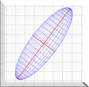
In figure 3 we show some examples of the equilibria at the critical turning point for QG+1 cyclonic and anticyclonic prolate vortices with  $h/r=2.5$ and
  $\beta =1$. As a result of the form of the background shear flow, the ellipsoid equilibrium axes are always either aligned with the coordinate axes or else tilted by an angle
  $\eta$ about the
  $x$-axis (see general configuration in figure 1). When
  $\theta =0^{\circ }$ the ellipsoidal axes are aligned with the coordinate axes, but as
  $\theta$ increases the equilibria tilt with respect to the coordinate axes. The anticyclonic equilibria are seemingly more tilted than the cyclonic ones. In figure 4 we make contour plots of the tilt angle
  $\eta (h/r,\theta )$ for the QG, QG+1 cyclonic and QG+1 anticyclonic cases at the critical turning point
  $\gamma _c$, for
  $\beta =1$. For all cases when the shear angle
  $\theta =0^{\circ }$ the ellipsoid axes are aligned with the coordinate axes. While oblate vortices are only slightly tilted for all values of
  $\theta$, the tilt angle for prolate vortices increases sharply with increasing
  $\theta$. Comparing the QG and QG+1 cases reveals that the QG+1 anticyclonic equilibria are generally more tilted than the QG equilibria, which in turn are more tilted than the cyclonic equilibria.

Figure 3. The ellipsoidal equilibria at the critical turning point for  $h/r=2.5$,
  $\beta =1$ and for different values of the angle
  $\theta$. The top row shows the QG+1 cyclonic cases and the bottom row shows the QG+1 anticyclonic cases.

Figure 4. Contour maps of the tilt angle  $\eta (h/r,\theta )$ for equilibria at the critical turning point
  $\gamma =\gamma _c$ with
  $\beta =1$ and showing (a) QG (black solid line) and QG+1 cyclonic (blue dashed) and (b) QG (black solid) and QG+1 anticyclonic (red dotted). The minimum and maximum contour values displayed are
  $0^{\circ }$ and
  $40^{\circ }$ respectively, and the contour interval is
  $10^{\circ }$. The contour corresponding to
  $\eta =0^{\circ }$ lies along the axis
  $\theta = 0^{\circ }$, and thus cannot be seen. The
  $\eta =40^{\circ }$ contour level is indicated.
3.1. Opposite-signed interactions ( $\beta < 1$)

Here, we present the results for opposite-signed interactions ( $\beta <1$). We begin by analysing how the turning point and marginal ellipsoidal instabilities are affected by changes in the parameters
  $\beta$,
  $\theta$ and
  $h/r$, while keeping PV and the Prandtl ratio fixed with
  $|\varpi |=0.5$ and
  $f/N=0.1$, respectively. In figure 5 we show contour plots of
  $|\gamma _m(\beta ,\theta )|$ and
  $|\gamma _c(\beta ,\theta )|$ for QG and QG+1 cyclonic (a,c,e,g,i) and QG and QG+1 anticyclonic (b,d,f,h,j) cases and for different height-to-width aspect ratios. Notably, in all cases the magnitude of the marginal and turning point strain values increase as
  $\beta \to 1$, implying that interactions between vortices of extremely different strengths are least destructive. For the most oblate case (
 $h/r=0.4$) there are no ellipsoidal instabilities before the critical turning point. Instabilities erupt as the aspect ratio increases for a certain range of parameter space, with generally the gap between
  $|\gamma _m|$ and
  $|\gamma _c|$ increasing with the aspect ratio. The occurrence of a marginal instability before the critical turning point strain coincides with the appearance of a kink in the curves for certain aspect ratios (for
  $h/r \ge 0.8$). This kink occurs when the matrix components
  $B_{11}=B_{22}$, i.e. when the principal axes
  $a$ and
  $b$ of the ellipsoid switch, as has been previously seen for the QG case in McKiver & Dritschel (Reference McKiver and Dritschel2006).

Figure 5. Contour plots of the magnitude of marginal and turning point strain rates as a function of  $\beta$ and
  $\theta$ in the case of opposite-signed interactions (
 $\beta <1$) and for QG and QG+1 cyclonic (a,c,e,g,i) and QG and QG+1 anticyclonic (b,d,f,h,j), with
  $\gamma ^{qg}_c$ (black thick solid),
  $\gamma ^{qg}_m$ (black dotted),
  $\gamma ^{cy}_c$ (blue thin solid),
  $\gamma ^{cy}_m$ (blue dashed),
  $\gamma ^{ac}_c$ (red thin solid) and
  $\gamma ^{ac}_m$ (red dashed). The two smallest contour values are indicated, with the maximum contour value being 0.1, and the contour interval is 0.005 for all plots.
For oblate vortices up to  $h/r=1$,
  $\gamma _c^{ac}>\gamma _c^{cy}$. This is the case also for prolate vortices, for values of
  $\theta$ below a certain value. However, for large
  $\theta$, the prolate cyclones are more stable than the anticyclones. For the most oblate case,
  $h/r=0.4$, the marginal strain increases with
  $\theta$. For
  $h/r=0.8$, where the kink appears in the curves, the marginal and turning point strains decrease with increasing
  $\theta$ (i.e. the troughs in the curves as a function of
  $\theta$). The range of
  $\theta$ values where this occurs increases with increasing aspect ratio. Let us refer to the angle which corresponds to the minimum absolute value of marginal strain as
  $\theta _m$. This is the vertical offset angle which is the most destructive. For
  $h/r=0.4$,
  $\theta ^{qg}_m=\theta ^{cy}_m=\theta ^{ac}_m=0^{\circ }$. While this is also the case for QG and QG+1 cyclonic equilibria with
  $h/r=0.8$, for QG+1 anticyclones
  $\theta _m\approx 75^{\circ }$. For
  $h/r=1$,
  $\theta _m^{cy}=0$, while
  $\theta _m^{qg}$ and
  $\theta _m^{ac}$ are between
  $65^{\circ }$ and
  $70^{\circ }$. At higher aspect ratios
  $\theta _m> 50^{\circ }$ for all cases, with generally
  $\theta ^{cy}_m\le \theta ^{qg}_m \le \theta ^{ac}_m$.
To determine what aspect ratio is most stable we will use the mean inverse strain rate as introduced by Reinaud et al. (Reference Reinaud, Dritschel and Koudella2003) where
 \begin{equation} \overline{\lambda_c} = \frac{2}{\rm \pi} \int_0^{{\rm \pi}/2} \lambda_c(\theta) \, \textrm{d} \theta,\end{equation}
where  $\lambda _c$ is the inverse of the critical strain rate. Similarly, we can define this also for the marginal strain
 \begin{equation} \overline{\lambda_m} = \frac{2}{\rm \pi} \int_0^{{\rm \pi}/2} \lambda_m(\theta) \, \textrm{d} \theta, \end{equation}
where now  $\lambda _m$ is the inverse of the marginal strain rate. As the value of
  $\theta$ in a turbulent flow varies randomly, the average of the inverse strain rate acts as a measure of the robustness of a family of vortices, with the parameters with the smallest value of
  $\lambda _c$ being the most robust. In figure 6 we show the marginal and critical average strain rates for the QG and QG+1 cyclonic and anticyclonic cases. The most robust QG equilibria tend to have aspect ratios slightly greater than 1.0, as was found by Reinaud et al. (Reference Reinaud, Dritschel and Koudella2003). The QG+1 cyclonic equilibria have higher aspect ratios, of around 1.25, shifting to above 1.4 for increasing
  $\beta$. On the other hand, the anticyclonic equilibria tend to be shorter, with aspect ratios of 1. When we look at the marginal average inverse strain, all the most stable aspect ratios are reduced, with QG centred at
  $h/r=1$, while the cyclonic and anticyclonic ones are just above and below that, respectively.

Figure 6. Plots of the critical turning point and marginal average inverse strain rates,  $\lambda _c$ in (a) and (b),
  $\lambda _m$ in (c) and (d) as a function of the aspect ratio
  $h/r$ in the case of opposite-signed interactions (
 $\beta <1$) for QG and QG+1 cyclonic (a,c) and QG and QG+1 anticyclonic (b,d). The QG values are depicted with thick solid curves, while the QG+1 cyclonic and anticyclonic values are depicted with dashed blue and dashed red curves respectively. The 5 curves shown are for
  $\beta =-4,-3,-2,-1,0$ with the
  $\beta =-4$ and
  $\beta =0$ curves indicated. The minimum of each curve is indicated with black triangles (QG), blue crosses (QG+1 cyclonic) and red crosses (QG+1 anticyclonic).
Now we look at how the equilibria are affected by changes in the PV anomaly, or in other words the PV-based Rossby number. In figure 7 we consider the case  $\beta =0$, i.e. equal and opposite interactions (
 $\kappa _b=-\kappa _v$), where we plot the magnitude of the marginal and turning point strain rates vs the potential vorticity for oblate (a,c,e) and prolate (b,d,f) equilibria with
  $h/r=0.6$ and
  $h/r=1.67$, respectively, each for three different values of the angle
  $\theta$. As the magnitude of the PV increases the magnitude of the marginal and turning point strain increases, i.e. the stronger the PV the more the vortex is able to resist the effect of the background flow. However, the behaviour is not the same for the QG and QG+1 cases. The QG lines are symmetric about the zero PV value, reflecting the fact that cyclonic and anticyclonic vortices behave the same at first order in the Rossby number. For low values of
  $|\varpi |$, less than approximately 0.25, QG+1 is similar to QG. However, an asymmetry between cyclonic and anticyclonic equilibria appears at the next order as the magnitude of the PV gets higher. The dependence of
  $\gamma _m$ and
  $\gamma _c$ on
  $h/r$ and
  $\theta$ corresponds with what was already seen in figure 5, with oblate ellipsoids having
  $\gamma _m=\gamma _c$, while for prolate ellipsoids there is a gap between
  $\gamma _m$ and
  $\gamma _c$ for certain
  $\theta$ values (figure 7b,d). However, for the anticyclonic prolate ellipsoids, the gap between
  $\gamma _m$ and
  $\gamma _c$ increases as
  $|\varpi |$ increases. This can lead to the anticyclonic equilibria becoming more unstable than the cyclonic case as
  $|\varpi |$ increases, whereas generally when there is no marginal instability before the turning point the cyclonic equilibria are more unstable than the anticyclonic ones.

Figure 7. Plot of the magnitude of the marginal and turning point strain rates as a function of the PV anomaly  $\varpi$ for an oblate (a,c,e) and prolate (b,d,f) ellipsoid with
  $h/r=0.6$ and
  $h/r=1.67$, respectively, and for
  $\theta =0^{\circ }$ (a,b),
  $\theta =30^{\circ }$ (c,d) and
  $\theta =60^{\circ }$ (e,f). The curves shown represent
  $\gamma ^{qg}_c$ (black solid line),
  $\gamma ^{qg}_m$ (black dashed line),
  $\gamma ^{cy}_c$ (blue solid line),
  $\gamma ^{cy}_m$ (blue pluses),
  $\gamma ^{ac}_c$ (red solid line) and
  $\gamma ^{ac}_m$ (red dots).
We now examine the impact of the Prandtl ratio  $f/N$ on the marginal and turning point strain. Here, we have computed equilibria and their stability for the range
  $0 < f/N \le 1$ in increments of
  $0.05$, while keeping the magnitude of the PV fixed at
  $|\varpi |=0.5$. We do this for a selection of the background flow parameters:
  $h/r=0.6, 1.67$ and
  $\theta =30^{\circ }, 60^{\circ }$. Note, we do not consider
  $\theta =0^{\circ }$ as the only terms in the background flow matrix, (2.26), where
  $f/N=1/\chi$ appears depend on the sine of
  $\theta$. In figure 8 we show results for
  ${\beta =0}$. At first order there is no dependence on
  $f/N$, although we include the QG case in the figures to provide a comparison with the next order. At the next order, changes in
  $f/N$ can influence the marginal and critical strain, although generally only weakly. For the oblate cases (figure 8a,c), increasing
  $f/N$ increases the cyclonic critical strain, while decreasing the anticyclonic strain, however these changes in the critical strain are very weak. For
  $\theta =60^{\circ }$ an instability in the anticyclonic equilibria appears, with the margin of instability decreasing more significantly as
  $f/N \to 1$, although remaining greater than the QG critical strain value. For the prolate cases (figure 8b,d) there is very different behaviour depending on the angle
  $\theta$. For
  $\theta =30^{\circ }$ we have a similar weak change in the critical strain, but now there is instability before the turning point for both cyclonic and anticyclonic equilibria. For
  $\theta =60^{\circ }$ the dependence on
  $f/N$ is far more dramatic, with a situation where the changes in
  $f/N$ results in a cross-over of the
  $\gamma _c^{cy}$ and
  $\gamma _c^{ac}$ curves, with cyclonic vortices being more stable than anticyclonic eddies for small values of
  $f/N$, but becoming more unstable above a certain threshold (
 $f/N \approx 0.7$).

Figure 8. Plot of the magnitude of the marginal and turning point strain rates as a function of  $f/N$ for an oblate (a,c) and prolate (b,d) ellipsoid with
  $h/r=0.6$ and
  $h/r=1.67$, respectively, and for
  $\theta =30^{\circ }$ (a,b) and
  $\theta =60^{\circ }$ (c,d). The curves shown represent
  $\gamma ^{qg}_c$ (black solid line),
  $\gamma ^{qg}_m$ (black dashed line),
  $\gamma ^{cy}_c$ (blue solid line),
  $\gamma ^{cy}_m$ (blue pluses),
  $\gamma ^{ac}_c$ (red solid line) and
  $\gamma ^{ac}_m$ (red dots).
3.2. Like-signed interactions ($\beta \ge 1$)

We now turn to the case of like-signed vortex interactions, first considering the dependence on  $\beta$,
  $\theta$ and
  $h/r$, while keeping PV and the Prandtl ratio fixed with
  $|\varpi |=0.5$ and
  $f/N=0.1$, respectively. In figure 9 we show contour plots of
  $|\gamma _m(\beta ,\theta )|$ and
  $|\gamma _c(\beta ,\theta )|$ in the case of like-signed interactions, comparing QG with QG+1 cyclonic (a,c,e,g,i) and QG with QG+1 anticyclonic (b,d,f,h,j) for a few different height-to-width aspect ratios. For all cases there appears to be no ellipsoidal instabilities before the critical turning point. In fact, these do occur, but only for
  $\theta =0^{\circ }$, as has been seen before for the QG case (McKiver & Dritschel Reference McKiver and Dritschel2006). As is the case for opposite-signed interactions the critical strain rates increase as
  $\beta \to 1$. For oblate vortices (
 $h/r \le 1$)
  $\gamma _c^{cy}<\gamma _c^{qg}<\gamma _c^{ac}$, with cyclonic equilibria more unstable than anticyclonic ones. The aspect ratio
  $h/r=1.25$ seems to be a threshold with
  $\gamma _c^{cy} \approx \gamma _c^{qg} \approx \gamma _c^{ac}$, beyond which anticyclonic vortices are more unstable than cyclonic ones. For
  $h/r=0.4$ the critical and marginal strain rates increase with increasing
  $\theta$, while for higher aspect ratios there are intermediate values of
  $\theta$ for which the vortex is more unstable, appearing as troughs in the curves as a function of
  $\theta$. These minimum strain values usually occur for
  $\theta$ between
  $20^{\circ }$ and
  $30^{\circ }$ for both QG and QG+1 models, and like the case of opposite-signed interactions
  $\theta ^{cy}_m\le \theta ^{qg}_m \le \theta ^{ac}_m$ for oblate vortices. However, for prolate vortices (
 $h/r \ge 1.25$),
  $\theta ^{cy}_m \approx \theta ^{ac}_m$.

Figure 9. As in figure 5 but now for the case of like-signed interactions ( $\beta \ge 1$). The two smallest contour values are indicated, with the maximum contour value being 0.1, and the contour interval is 0.005 for all plots.
As was done for the opposite-signed interactions, here, we compute the average inverse critical strain rates to see what aspect ratios are most resilient in like-signed interactions (figure 10). Note, for like-signed interactions this is the same as the average marginal inverse strain rate as  $\gamma _m=\gamma _c$. As observed by Reinaud et al. (Reference Reinaud, Dritschel and Koudella2003), QG vortices tend to be slightly oblate, with an aspect ratio of
  $0.8 f/N$ as
  $\beta \to 1$. At the next order, anticyclonic vortices are even more oblate (
 $h/r \approx 0.7 f/N$) for
  $\beta =1$, while cyclonic vortices have a higher aspect ratio, approaching unity (
 $h/r \approx f/N$).

Figure 10. Plots of the critical turning point average inverse strain rates  $\lambda _c$ as a function of the aspect ratio
  $h/r$ in the case of like-signed interactions (
 $\beta \ge 1$) for QG and QG+1 cyclonic (a) and QG and QG+1 anticyclonic (b). The 6 curves shown are for
  $\beta =1,2,3,4,5,6$ with
  $\beta =1$ and
  $\beta =6$ indicated. The minimum of each curve is indicated with black triangles (QG), blue crosses (QG+1 cyclonic) and red crosses (QG+1 anticyclonic).
Next, we show the dependence on the anomalous PV. In figure 11 we consider the case  $\beta =2$, i.e. equal interactions (
 $\kappa _b=\kappa _v$), where we plot the marginal and turning point strain vs
  $\varpi$ for the case of an oblate and prolate vortex with
  $h/r=0.6$ and
  $h/r=1.67$, respectively, and for three different values of the angle
  $\theta$. Like the case of opposite-signed interactions, as
  $|\varpi |$ increases the magnitude of the marginal and critical strain increases. For the case of oblate vortices the anticyclonic equilibria become more stable while the cyclonic equilibria become more unstable as
  $|\varpi |$ increases. Conversely, for prolate vortices, the cyclonic equilibria become more stable while the anticyclonic equilibria become more unstable as
  $|\varpi |$ increases. The only case where marginal instability occurs before the critical turning point is for the prolate vortex with
  $\theta =0^{\circ }$. As was seen for the opposite-signed interaction for the anticyclonic equilibria the gap between marginal and critical strain increases with
  $|\varpi |$, leading to the anticyclonic equilibria becoming more unstable than the cyclonic one. Overall, the magnitude of the critical strain values for like-signed interactions are much smaller than the values for the opposite-signed interactions seen in figure 7, implying that the like-signed interactions are more destructive.

Figure 11. As in figure 7 but now for like-signed interactions with  $\beta =2$.
In figure 12 we show the marginal and critical strain as a function of  $f/N$ for the case
  $\beta =2$. For the oblate cases (figure 12a,c)
  $\gamma _c^{ac}>\gamma _c^{cy}$, but increases in
  $f/N$ leads to increases in the gap between the turning point of the cyclonic and anticyclonic vortices, i,e. stabilising anticyclones while destabilising cyclones. For the prolate cases (figure 12b,d), we see a cross-over of
  $\gamma _m^{cy}$ and
  $\gamma _m^{ac}$ curves, with cyclonic vortices being more stable than anticyclonic vortices for small values of
  $f/N$, but becoming more unstable above a certain threshold. This threshold is affected by the offset angle
  $\theta$, moving from
  $f/N \approx 0.65$ for
  $\theta =30^{\circ }$ to
  $f/N \approx 0.55$ for
  $\theta =60^{\circ }$. Overall increases in
  $f/N$ act to stabilise anticyclonic ellipsoids, while destabilising cyclonic ones. The location of this cross-over is linked to the tilt angle of the equilibria, with the cyclonic equilibria becoming more unstable when their tilt angle is greater than the tilt angle of the anticyclonic equilibria.

Figure 12. As in figure 8 but now for like-signed interactions with  $\beta =2$.
4. Discussion and conclusions
Here, we presented results for the equilibria of an ellipsoidal vortex in a background shear flow at the next order to QG. These results give a glimpse of the characteristics of vortices that are most resistant to the influence of their surroundings at finite Rossby number.
Considering first the impact of the background flow parameter  $\beta$ defined in (2.25) as the ratio of vortex strengths, we found that for both QG+1 cyclones and anticyclones the most stable equilibria occur as
  $\beta \to 1$. This is what has been previously found for QG (Reinaud et al. Reference Reinaud, Dritschel and Koudella2003; McKiver & Dritschel Reference McKiver and Dritschel2006) and implies that interactions between vortices of very different strengths (
 $\beta =1$) are the most stable.
Next, considering the parameter  $\theta$, we find that when there is vertical shear (
 $\theta >0^{\circ }$) prolate equilibria are tilted about the
  $x$-axis with respect to the vertical, with anticyclonic equilibria more tilted than cyclonic ones. The value of
  $\theta$ for which
  $|\gamma |$ is minimum indicates the offset angle which is most destructive. We have found that generally this offset angle tends to be greater for anticyclonic equilibria than cyclonic ones. This reflects the findings of Reinaud & Dritschel (Reference Reinaud and Dritschel2018), where they analysed the merger of two corotating vortices at finite Rossby number and found that nearly aligned cyclones tend to merge from further apart than anticyclones, while vertically offset anticyclones merge from further apart than cyclones.
In general, we have found that the most resilient cyclonic vortices are slightly prolate, while anticyclonic vortices tend to be more oblate (where the height is scaled by  $f/N$), with respect to the QG equivalent cases. This tendency increases with the Rossby number. Previous studies based on QG theory had already established that QG vortices tend to be oblate, due to the fact that vertical shear is more destabilising than horizontal shear (Reinaud & Dritschel Reference Reinaud and Dritschel2002; Reinaud et al. Reference Reinaud, Dritschel and Koudella2003). The work of Graves, McWilliams & Montgomery (Reference Graves, McWilliams and Montgomery2006) considering gradient-wind balance in the shallow water equations studied the impact of a straining flow on cyclonic and anticyclonic vortices at finite Rossby number, finding that strain weakens cyclonic vortices significantly more than anticyclonic vortices at higher Rossby numbers. The work by Reinaud & Dritschel (Reference Reinaud and Dritschel2018) considering two vortex merger for the full 3-D non-hydrostatic equations also finds that cyclonic vortices are more susceptible to horizontal strain than anticyclonic vortices, but also finds that anticyclonic vortices are more adversely affected by vertical shear given that vertically offset anticyclones merge from further apart than cyclones. These previous studies all point to the fact that the most resilient anticyclonic vortices must adopt a more oblate shape to resist the impact of vertical shear, while cyclonic vortices must reduce the impact of strain by in turn reducing their mean horizontal radius, becoming more prolate, as is found in this work. These findings also agree qualitatively with other theoretical and modelling studies (Hassanzadeh, Marcus & Le Gal Reference Hassanzadeh, Marcus and Le Gal2012; Damien et al. Reference Damien, Bosse, Testor, Marsaleix and Estournel2017; Lemasquerier et al. Reference Lemasquerier, Facchini, Favier and Le Bars2020; Xu et al. Reference Xu, Yu, Nan and Ren2020) and observations of subsurface vortices (Bosse et al. Reference Bosse2016; Dilmahamod et al. Reference Dilmahamod, Aguiar-González, Penven, Reason, De Ruijter, Malan and Hermes2018). Further observational studies would be needed to comprehensively catalogue the typical size, shape and orientation of subsurface cyclonic and anticyclonic eddies.
We also examined the dependence of the equilibria on the Prandtl ratio  $f/N$. We found that, for prolate vortices, increasing
  $f/N$ can change from a regime where cyclones are more stable, to one where anticyclones are. The value of
  $f/N$ where this occurs depends on the offset angle
  $\theta$, decreasing as
  $\theta$ increases. Although, overall, these values of
  $f/N$ are large, they are still within the values for which the flow is statically stable, based on the empirical formula found by Dritschel & McKiver (Reference Dritschel and McKiver2015) from their study of turbulence simulations at different values of the Rossby and Prandtl ratio. This effect, along with the fact that oblate vortices tend to be anticyclonic, may lead to the overall dominance of anticyclonic eddies in geophysical flows (Graves et al. Reference Graves, McWilliams and Montgomery2006) and may even have relevance for the typical structure found for extraplanetary vortices (Abrahamyan Reference Abrahamyan2016; Lemasquerier et al. Reference Lemasquerier, Facchini, Favier and Le Bars2020; Sánchez-Lavega et al. Reference Sánchez-Lavega2021).
Here, we have computed the second-order (ellipsoidal) stability modes, modes which deform the vortex while preserving its ellipsoidal form. In future work, it would be useful to solve the full stability problem, as was done by Hashimoto et al. (Reference Hashimoto, Shimonishi and Miyazaki1999) and McKiver & Dritschel (Reference McKiver and Dritschel2006) for QG, where it was revealed that the marginal modes are almost entirely ellipsoidal. However, the complexity of the equations for the QG+1 ellipsoid make the solution to the full linear stability problem much more challenging. While such a study would reveal if there might be marginal non-ellipsoidal modes, this would not affect the value of the critical turning point strain that was computed here.
This work has underlined the differences between cyclonic and anticyclonic ellipsoidal vortices at the next order to QG. In future work, the full non-hydrostatic equations could be solved numerically, to perform high resolution turbulence simulations in order to obtain statistics on the most typical vortex characteristics, as was done by Reinaud et al. (Reference Reinaud, Dritschel and Koudella2003) for the QG model. Also, further work could be done to extend the single QG+1 ellipsoidal vortex model to a multi-vortex model, as was done by Dritschel, Reinaud & McKiver (Reference Dritschel, Reinaud and McKiver2004) for QG, which would provide a useful tool for understanding turbulence dynamics at finite Rossby number.
Acknowledgements
The author would like to thank J. Reinaud for helpful comments, as well as comments provided by two anonymous reviewers.
Declaration of interest
The authors report no conflict of interest.
Appendix A. Derivative of the self-induced flow matrix
Here, we show how to determine the derivative of the self-induced flow matrix  ${\boldsymbol {S}}_v={\boldsymbol {L}}_{\varphi } \boldsymbol {\varGamma }_v^{(2)} + {\boldsymbol {L}}_{\psi } \boldsymbol {\varPsi }_v^{(2)} + {\boldsymbol {L}}_{\phi } (\boldsymbol {\varPhi }_v^{(1)}+\boldsymbol {\varPhi }_v^{(2)})$ with respect to the elements of the matrix
  ${\boldsymbol {B}}$. As the matrices
  ${\boldsymbol {L}}$ are constant matrices, we only need to determine the derivative of the symmetric matrices
  $\boldsymbol {\varGamma }_v$,
  $\boldsymbol {\varPsi }_v$ and
  $\boldsymbol {\varPhi }_v$, all of which have the same general form, i.e.
 \begin{equation} \boldsymbol{\varPhi} = {\boldsymbol{M}} {\boldsymbol{H}} {\boldsymbol{M}}^{\rm T}.\end{equation}
This general form can be rewritten as
 \begin{align} \boldsymbol{\varPhi} &= {\boldsymbol{H}}_{11} \hat{\boldsymbol a} \hat{\boldsymbol a}^{\rm T} + {\boldsymbol{H}}_{22} \hat{\boldsymbol b} \hat{\boldsymbol b}^{\rm T} + {\boldsymbol{H}}_{33} \hat{\boldsymbol c} \hat{\boldsymbol c}^{\rm T} + {\boldsymbol{H}}_{12} (\hat{\boldsymbol a} \hat{\boldsymbol b}^{\rm T} + \hat{\boldsymbol b} \hat{\boldsymbol a}^{\rm T} ) + {\boldsymbol{H}}_{31} (\hat{\boldsymbol c} \hat{\boldsymbol a}^{\rm T} + \hat{\boldsymbol a} \hat{\boldsymbol c}^{\rm T} ) \nonumber\\ &\quad + {\boldsymbol{H}}_{23} (\hat{\boldsymbol b} \hat{\boldsymbol c}^{\rm T} + \hat{\boldsymbol c} \hat{\boldsymbol b}^{\rm T} ). \end{align}
Taking the derivatives with respect to the  ${\boldsymbol {B}}$ matrix elements
  $B^k$ gives,
 \begin{align} {\frac{{\partial} \boldsymbol{\varPhi}}{{\partial} B^k} }&= {\frac{{\partial} {\boldsymbol{H}}_{11}}{{\partial} B^k} }\hat{\boldsymbol a} \hat{\boldsymbol a}^{\rm T} + {\boldsymbol{H}}_{11} \left({\frac{{\partial} \hat{\boldsymbol a}}{{\partial} B^k} } \hat{\boldsymbol a}^{\rm T}+ \hat{\boldsymbol a} {\frac{{\partial} \hat{\boldsymbol a}^{\rm T}}{{\partial} B^k} } \right) + {\frac{{\partial} {\boldsymbol{H}}_{22}}{{\partial} B^k} }\hat{\boldsymbol b} \hat{\boldsymbol b}^{\rm T} + {\boldsymbol{H}}_{22} \left({\frac{{\partial} \hat{\boldsymbol b}}{{\partial} B^k} } \hat{\boldsymbol b}^{\rm T}+ \hat{\boldsymbol b} {\frac{{\partial} \hat{\boldsymbol b}^{\rm T}}{{\partial} B^k} } \right) \nonumber\\ &\quad + {\frac{{\partial} {\boldsymbol{H}}_{33}}{{\partial} B^k} }\hat{\boldsymbol c} \hat{\boldsymbol c}^{\rm T} + {\boldsymbol{H}}_{33} \left({\frac{{\partial} \hat{\boldsymbol c}}{{\partial} B^k} } \hat{\boldsymbol c}^{\rm T}+ \hat{\boldsymbol c} {\frac{{\partial} \hat{\boldsymbol c}^{\rm T}}{{\partial} B^k} } \right) \nonumber\\ &\quad + {\frac{{\partial} {\boldsymbol{H}}_{12}}{{\partial} B^k} }(\hat{\boldsymbol a} \hat{\boldsymbol b}^{\rm T} + \hat{\boldsymbol b} \hat{\boldsymbol a}^{\rm T} )+{\boldsymbol{H}}_{12}\left({\frac{{\partial} \hat{\boldsymbol a}}{{\partial} B^k} }\hat{\boldsymbol b}^{\rm T} + \hat{\boldsymbol a} {\frac{{\partial} \hat{\boldsymbol b}^{\rm T}}{{\partial} B^k} } + {\frac{{\partial} \hat{\boldsymbol b}}{{\partial} B^k} } \hat{\boldsymbol a}^{\rm T} + \hat{\boldsymbol b} {\frac{{\partial} \hat{\boldsymbol a}^{\rm T}}{{\partial} B^k} } \right) \nonumber\\ &\quad + {\frac{{\partial} {\boldsymbol{H}}_{31}}{{\partial} B^k} }(\hat{\boldsymbol c} \hat{\boldsymbol a}^{\rm T} + \hat{\boldsymbol a} \hat{\boldsymbol c}^{\rm T} )+{\boldsymbol{H}}_{31}\left({\frac{{\partial} \hat{\boldsymbol c}}{{\partial} B^k} }\hat{\boldsymbol a}^{\rm T} + \hat{\boldsymbol c} {\frac{{\partial} \hat{\boldsymbol a}^{\rm T}}{{\partial} B^k} } + {\frac{{\partial} \hat{\boldsymbol a}}{{\partial} B^k} } \hat{\boldsymbol c}^{\rm T} + \hat{\boldsymbol a} {\frac{{\partial} \hat{\boldsymbol c}^{\rm T}}{{\partial} B^k} } \right) \nonumber\\ &\quad + {\frac{{\partial} {\boldsymbol{H}}_{23}}{{\partial} B^k} }(\hat{\boldsymbol b} \hat{\boldsymbol c}^{\rm T} + \hat{\boldsymbol c} \hat{\boldsymbol b}^{\rm T} )+{\boldsymbol{H}}_{31}\left({\frac{{\partial} \hat{\boldsymbol b}}{{\partial} B^k} }\hat{\boldsymbol c}^{\rm T} + \hat{\boldsymbol b} {\frac{{\partial} \hat{\boldsymbol c}^{\rm T}}{{\partial} B^k} } + {\frac{{\partial} \hat{\boldsymbol c}}{{\partial} B^k} } \hat{\boldsymbol b}^{\rm T} + \hat{\boldsymbol c} {\frac{{\partial} \hat{\boldsymbol b}^{\rm T}}{{\partial} B^k} } \right). \end{align}
For the derivatives of the axis vectors we can use formulas derived in McKiver & Dritschel (Reference McKiver and Dritschel2006), i.e.
 $$\begin{gather} {\frac{{\partial} \hat{\boldsymbol a}}{{\partial} B^k} } = \lambda^k_{ab} \hat{\boldsymbol b} - \lambda^k_{ca} \hat{\boldsymbol c}, \end{gather}$$
 $$\begin{gather}{\frac{{\partial} \hat{\boldsymbol b}}{{\partial} B^k} } = \lambda^k_{bc} \hat{\boldsymbol c} - \lambda^k_{ab} \hat{\boldsymbol a}, \end{gather}$$
 $$\begin{gather}{\frac{{\partial} \hat{\boldsymbol c}}{{\partial} B^k} } = \lambda^k_{ca} \hat{\boldsymbol a} - \lambda^k_{bc} \hat{\boldsymbol b}, \end{gather}$$
where we have the following scalars:
 $$\begin{gather} \lambda^k_{ab} = \frac{\hat{\boldsymbol a}^{\rm T} {\boldsymbol{J}}^k \hat{\boldsymbol b}}{a^2-b^2}, \end{gather}$$
 $$\begin{gather}\lambda^k_{bc} = \frac{\hat{\boldsymbol b}^{\rm T} {\boldsymbol{J}}^k \hat{\boldsymbol c}}{b^2-c^2}, \end{gather}$$
 $$\begin{gather}\lambda^k_{ca} = \frac{\hat{\boldsymbol c}^{\rm T} {\boldsymbol{J}}^k \hat{\boldsymbol a}}{c^2-a^2}. \end{gather}$$
As the matrices  ${\boldsymbol {H}}$ depend on the coefficients
  $\xi _a$,
  $\xi _b$,
  $\xi _c$ their derivatives can be obtained, again using formulas from McKiver & Dritschel (Reference McKiver and Dritschel2006), namely
 $$\begin{gather} {\frac{{\partial} \xi_a}{{\partial} B^k} } = \hat{\boldsymbol a}^{\rm T} {\boldsymbol{J}}^k \hat{\boldsymbol a} {\frac{{\partial} \xi_a}{{\partial} a^2} } +\hat{\boldsymbol b}^{\rm T} {\boldsymbol{J}}^k \hat{\boldsymbol b} {\frac{{\partial} \xi_a}{{\partial} b^2} } +\hat{\boldsymbol c}^{\rm T} {\boldsymbol{J}}^k \hat{\boldsymbol c} {\frac{{\partial} \xi_a}{{\partial} c^2} }, \end{gather}$$
 $$\begin{gather}{\frac{{\partial} \xi_b}{{\partial} B^k} } = \hat{\boldsymbol a}^{\rm T} {\boldsymbol{J}}^k \hat{\boldsymbol a} {\frac{{\partial} \xi_b}{{\partial} a^2} } +\hat{\boldsymbol b}^{\rm T} {\boldsymbol{J}}^k \hat{\boldsymbol b} {\frac{{\partial} \xi_b}{{\partial} b^2} } +\hat{\boldsymbol c}^{\rm T} {\boldsymbol{J}}^k \hat{\boldsymbol c} {\frac{{\partial} \xi_b}{{\partial} c^2} }, \end{gather}$$
 $$\begin{gather}{\frac{{\partial} \xi_c}{{\partial} B^k} } = \hat{\boldsymbol a}^{\rm T} {\boldsymbol{J}}^k \hat{\boldsymbol a} {\frac{{\partial} \xi_c}{{\partial} a^2} } +\hat{\boldsymbol b}^{\rm T} {\boldsymbol{J}}^k \hat{\boldsymbol b} {\frac{{\partial} \xi_c}{{\partial} b^2} } +\hat{\boldsymbol c}^{\rm T} {\boldsymbol{J}}^k \hat{\boldsymbol c} {\frac{{\partial} \xi_c}{{\partial} c^2} }, \end{gather}$$
where the derivatives of the coefficients  $\xi _a$,
  $\xi _b$,
  $\xi _c$ are
 $$\begin{gather} {\frac{{\partial} \xi_a}{{\partial} a^2} }={-}\frac{(\varOmega_{ab}+\varOmega_{ca})}{2a^2}, \quad {\frac{{\partial} \xi_a}{{\partial} b^2} }=\frac{\varOmega_{ab}}{2b^2},\quad {\frac{{\partial} \xi_a}{{\partial} c^2} }=\frac{\varOmega_{ca}}{2c^2}, \end{gather}$$
 $$\begin{gather}{\frac{{\partial} \xi_b}{{\partial} b^2} }={-}\frac{(\varOmega_{bc}+\varOmega_{ab})}{2b^2}, \quad {\frac{{\partial} \xi_b}{{\partial} c^2} }=\frac{\varOmega_{bc}}{2c^2},\quad {\frac{{\partial} \xi_b}{{\partial} a^2} }=\frac{\varOmega_{ab}}{2a^2}, \end{gather}$$
 $$\begin{gather}{\frac{{\partial} \xi_c}{{\partial} c^2} }={-}\frac{(\varOmega_{ca}+\varOmega_{bc})}{2c^2}, \quad {\frac{{\partial} \xi_c}{{\partial} a^2} }=\frac{\varOmega_{ca}}{2a^2},\quad {\frac{{\partial} \xi_c}{{\partial} b^2} }=\frac{\varOmega_{bc}}{2b^2}. \end{gather}$$
Finally, (A3) can be rewritten in the form
 \begin{equation} {\frac{{\partial} \boldsymbol{\varPhi}}{{\partial} B^k} } = {\boldsymbol{M}} {\boldsymbol{Q}}^k {\boldsymbol{M}}^{\rm T},\end{equation}
where  ${\boldsymbol {Q}}^k$ are symmetric matrices whose components are given by
 $$\begin{gather} {\boldsymbol{Q}}^k_{11} = {\frac{{\partial} {\boldsymbol{H}}_{11}}{{\partial} B^k} }+2(\lambda_{ca}^k{\boldsymbol{H}}_{31}-\lambda_{ab}^k{\boldsymbol{H}}_{12}), \end{gather}$$
 $$\begin{gather}{\boldsymbol{Q}}^k_{22} = {\frac{{\partial} {\boldsymbol{H}}_{22}}{{\partial} B^k} }+2(\lambda_{ab}^k{\boldsymbol{H}}_{12}-\lambda_{bc}^k{\boldsymbol{H}}_{23}), \end{gather}$$
 $$\begin{gather}{\boldsymbol{Q}}^k_{33} = {\frac{{\partial} {\boldsymbol{H}}_{33}}{{\partial} B^k} }+2(\lambda_{bc}^k{\boldsymbol{H}}_{23}-\lambda_{ca}^k{\boldsymbol{H}}_{31}), \end{gather}$$
 $$\begin{gather}{\boldsymbol{Q}}^k_{12} = {\frac{{\partial} {\boldsymbol{H}}_{12}}{{\partial} B^k} }+\lambda_{ab}^k ({\boldsymbol{H}}_{11}-{\boldsymbol{H}}_{22})+\lambda_{ca}^k {\boldsymbol{H}}_{23}-\lambda_{bc}^k {\boldsymbol{H}}_{31}, \end{gather}$$
 $$\begin{gather}{\boldsymbol{Q}}^k_{31} = {\frac{{\partial} {\boldsymbol{H}}_{31}}{{\partial} B^k} }+\lambda_{ca}^k ({\boldsymbol{H}}_{33}-{\boldsymbol{H}}_{11})+\lambda_{bc}^k {\boldsymbol{H}}_{12}-\lambda_{ab}^k {\boldsymbol{H}}_{23}, \end{gather}$$
 $$\begin{gather}{\boldsymbol{Q}}^k_{23}={\frac{{\partial} {\boldsymbol{H}}_{23}}{{\partial} B^k} }+\lambda_{bc}^k ({\boldsymbol{H}}_{22}-{\boldsymbol{H}}_{33})+\lambda_{ab}^k {\boldsymbol{H}}_{31}-\lambda_{ca}^k {\boldsymbol{H}}_{12}. \end{gather}$$


