


1 Introduction
It is universally acknowledged that shock reflection is a fundamental phenomenon in supersonic flow, which exists widely in the internal and external flow fields of supersonic as well as hypersonic vehicles. Since Mach (Reference Mach1878) first studied two different shock reflection configurations, known as regular reflection (RR) and Mach reflection (MR), subsequent studies conducted by many researchers have never ceased. One of the hottest topics on reflection configurations is RR–MR transition, of which two classical criteria, the detachment criterion and the von Neumann criterion, were first proposed by von Neumann (Reference von Neumann1943, Reference von Neumann1945). The reflected shock solution is related to flow deflection angle and pressure. Kawamura & Satto (Reference Kawamura and Satto1956) therefore introduced shock polar lines, i.e. pressure–deflection polar lines, to helpfully illustrate and analyse the shock configurations, based on which Ben-Dor (Reference Ben-Dor1991) summarized the reflection phenomena in steady, pseudo-steady and unsteady flows.
Most researches have mainly been focused on flow structures containing a single incident shock as well as double symmetrical incident shocks, while the flow field generated by asymmetrical geometry and multiple incident shocks may be more common in practical engineering applications. For a flow structure generated by double opposite asymmetrical ramps in steady flow (see Ivanov et al.
Reference Ivanov, Ben-Dor, Elperin, Kudryavtes and Khotyanovsky2002), the possible shock reflections are schematically illustrated in figure 1. The overall RR configuration, as shown in figure 1(a), consists of double asymmetrical incident shocks, denoted by
 $I_{1}^{\prime }$
on the top ramp and
$I_{1}^{\prime }$
on the top ramp and
 $I_{1}$
on the bottom ramp, respectively, and double asymmetrical reflected shocks, denoted by
$I_{1}$
on the bottom ramp, respectively, and double asymmetrical reflected shocks, denoted by
 $R_{1}^{\prime }$
and
$R_{1}^{\prime }$
and
 $R_{1}$
, respectively. An overall RR boundary condition requires that all the incident and reflected shocks meet at a single node, and the accompanying flow defection angles across the shocks must fulfill the equation
$R_{1}$
, respectively. An overall RR boundary condition requires that all the incident and reflected shocks meet at a single node, and the accompanying flow defection angles across the shocks must fulfill the equation
 $$\begin{eqnarray}|\unicode[STIX]{x1D6FC}_{1}-\unicode[STIX]{x1D6FC}_{3}|=|\unicode[STIX]{x1D6FC}_{2}-\unicode[STIX]{x1D6FC}_{4}|=\unicode[STIX]{x1D6FC}_{r}.\end{eqnarray}$$
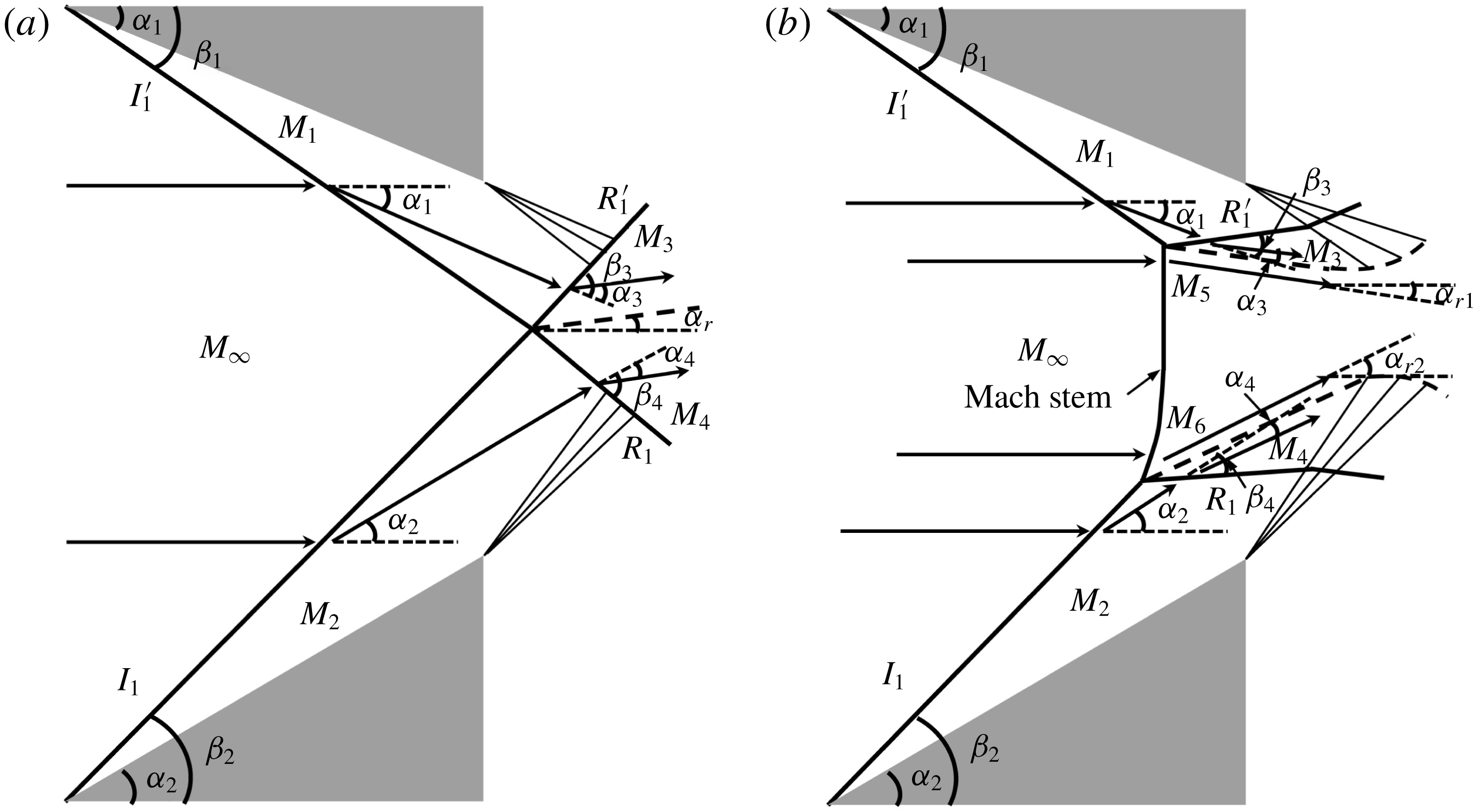
Figure 1. Schematic illustrations of possible shock reflections in steady flow: (a) overall RR, and (b) overall MR.
The overall MR, as shown in figure 1(b), is more complicated than the overall RR, of which a very strong curve shock, named Mach stem, is added to the configuration (see Azevedo & Liu Reference Azevedo and Liu1993; Tao et al. Reference Tao, Liu, Fan, Xiong, Yu and Sun2017). Accordingly, incident shocks and reflected shocks cannot meet at a single node, which will be replaced by two endpoints of the Mach stem. The boundary condition of an overall MR hence becomes
 $$\begin{eqnarray}\left.\begin{array}{@{}c@{}}|\unicode[STIX]{x1D6FC}_{1}-\unicode[STIX]{x1D6FC}_{3}|=\unicode[STIX]{x1D6FC}_{r1},\\ |\unicode[STIX]{x1D6FC}_{2}-\unicode[STIX]{x1D6FC}_{4}|=\unicode[STIX]{x1D6FC}_{r2}.\end{array}\right\}\end{eqnarray}$$
The solutions of asymmetrical shock reflection can be indicated by pressure–deflection polar lines, which are illustrated in figure 2. There,
 $I_{1}^{\prime }$
and
$I_{1}^{\prime }$
and
 $I_{1}$
are the incident shock polar lines on the top and bottom ramps, respectively, along which the pressure fulfills the oblique shock wave equations (see Ben-Dor Reference Ben-Dor1991; Li, Chpoun & Ben-Dor Reference Li, Chpoun and Ben-Dor1999). The solution of the reflected shock can be observed clearly by the intersection (denoted by point
$I_{1}$
are the incident shock polar lines on the top and bottom ramps, respectively, along which the pressure fulfills the oblique shock wave equations (see Ben-Dor Reference Ben-Dor1991; Li, Chpoun & Ben-Dor Reference Li, Chpoun and Ben-Dor1999). The solution of the reflected shock can be observed clearly by the intersection (denoted by point
 $a$
) of reflected shock polar lines, i.e.
$a$
) of reflected shock polar lines, i.e.
 $R_{1}^{\prime }$
and
$R_{1}^{\prime }$
and
 $R_{1}$
. Assuming that
$R_{1}$
. Assuming that
 $I_{1}^{\prime }$
remains stable, i.e. the reflected shock polar line of
$I_{1}^{\prime }$
remains stable, i.e. the reflected shock polar line of
 $I_{1}^{\prime }$
resides in
$I_{1}^{\prime }$
resides in
 $R_{1}^{\prime }$
, while the ramp angle of
$R_{1}^{\prime }$
, while the ramp angle of
 $I_{1}$
ranges from a small enough degree to a big enough degree, then the admissible reflected shock polar lines of
$I_{1}$
ranges from a small enough degree to a big enough degree, then the admissible reflected shock polar lines of
 $I_{1}$
can be represented by
$I_{1}$
can be represented by
 $R_{1}$
–
$R_{1}$
–
 $R_{5}$
. Here
$R_{5}$
. Here
 $R_{2}$
and
$R_{2}$
and
 $R_{4}$
are two such typical lines:
$R_{4}$
are two such typical lines:
 $I_{1}^{\prime }$
(or
$I_{1}^{\prime }$
(or
 $I_{1}$
, depending on
$I_{1}$
, depending on
 $\unicode[STIX]{x1D6FC}_{1}$
),
$\unicode[STIX]{x1D6FC}_{1}$
),
 $R_{1}^{\prime }$
and
$R_{1}^{\prime }$
and
 $R_{2}$
meet at a single point
$R_{2}$
meet at a single point
 $b$
;
$b$
;
 $R_{1}^{\prime }$
and
$R_{1}^{\prime }$
and
 $R_{4}$
are tangent at a single point
$R_{4}$
are tangent at a single point
 $d$
. According to the study conducted by Li et al. (Reference Li, Chpoun and Ben-Dor1999),
$d$
. According to the study conducted by Li et al. (Reference Li, Chpoun and Ben-Dor1999),
 $b$
and
$b$
and
 $d$
are the two criteria of overall RR to overall MR transition, of which the ramp angles
$d$
are the two criteria of overall RR to overall MR transition, of which the ramp angles
 $\unicode[STIX]{x1D6FC}^{vN}$
and
$\unicode[STIX]{x1D6FC}^{vN}$
and
 $\unicode[STIX]{x1D6FC}^{D}$
correspond to the von Neumann condition and the detachment condition, respectively. Accordingly, an overall RR solution resides in the domain where
$\unicode[STIX]{x1D6FC}^{D}$
correspond to the von Neumann condition and the detachment condition, respectively. Accordingly, an overall RR solution resides in the domain where
 $\unicode[STIX]{x1D6FC}_{2}<\unicode[STIX]{x1D6FC}^{vN}$
, such as
$\unicode[STIX]{x1D6FC}_{2}<\unicode[STIX]{x1D6FC}^{vN}$
, such as
 $R_{1}$
; an overall MR solution resides in the domain where
$R_{1}$
; an overall MR solution resides in the domain where
 $\unicode[STIX]{x1D6FC}_{2}>\unicode[STIX]{x1D6FC}^{D}$
, such as
$\unicode[STIX]{x1D6FC}_{2}>\unicode[STIX]{x1D6FC}^{D}$
, such as
 $R_{5}$
; while more than one analytic solution may reside in the domain where
$R_{5}$
; while more than one analytic solution may reside in the domain where
 $\unicode[STIX]{x1D6FC}^{vN}<\unicode[STIX]{x1D6FC}_{2}<\unicode[STIX]{x1D6FC}^{D}$
, such as
$\unicode[STIX]{x1D6FC}^{vN}<\unicode[STIX]{x1D6FC}_{2}<\unicode[STIX]{x1D6FC}^{D}$
, such as
 $R_{3}$
, which is known as the dual-solution domain (see Hu et al.
Reference Hu, Myong, Kim and Cho2009).
$R_{3}$
, which is known as the dual-solution domain (see Hu et al.
Reference Hu, Myong, Kim and Cho2009).
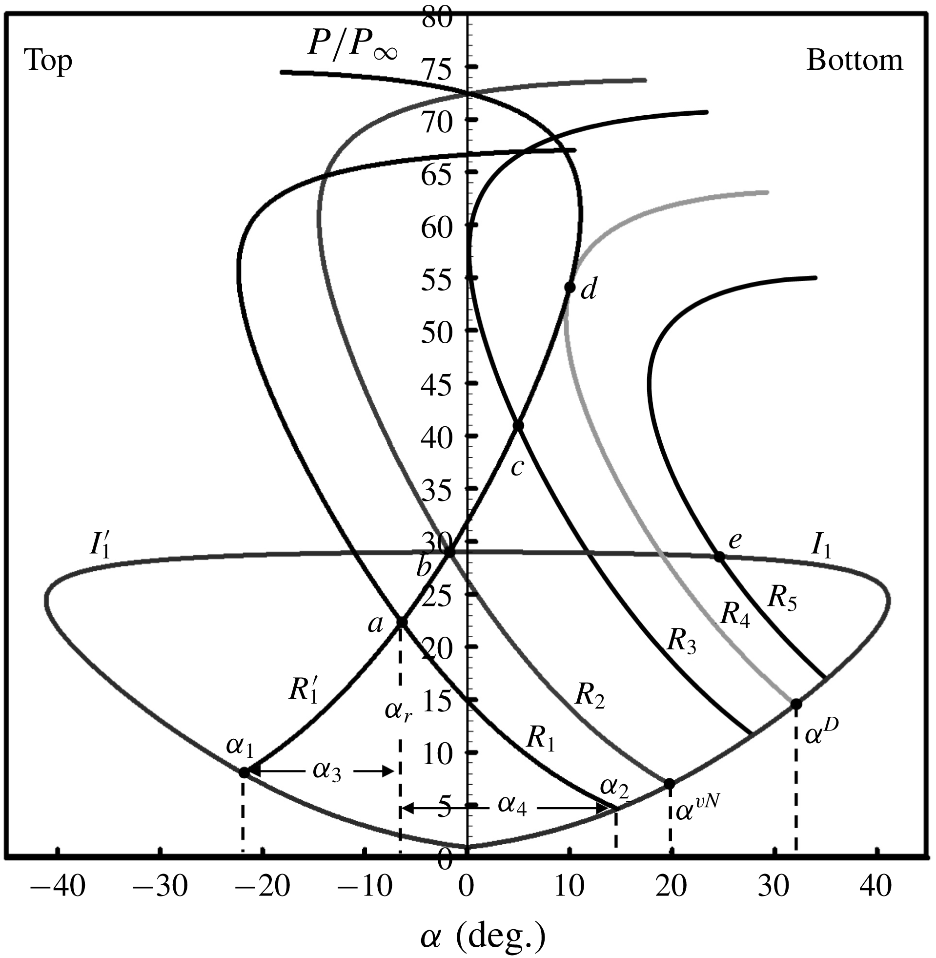
Figure 2. Pressure–deflection polar lines illustrating various possible solutions of asymmetric shock reflection in steady flows.
The RR–MR transition has been noticed for decades since some earlier research conducted by Hornung, Oertel & Sandeman (Reference Hornung, Oertel and Sandeman1979) and Hornung & Robinson (Reference Hornung and Robinson1982). However, it is still difficult to predict the reflected solution in the dual-solution domain, in which both the RR and MR configurations are stable. The second law of thermodynamics requires that a non-equilibrium state process will be in the direction of increasing entropy. As a supplement, the a posteriori axiom postulated by Glansdorff & Prigogine (Reference Glansdorff and Prigogine1971) points out that the process must fulfill the principle of minimum entropy production, based on which Li & Ben-Dor (Reference Li and Ben-Dor1996a ,Reference Li and Ben-Dor b ) proposed new criteria of RR–MR transition in steady as well as unsteady flow, which agreed well with the experimental results obtained by Chpoun et al. (Reference Chpoun, Passerel, Li and Ben-Dor1995). Most of the theoretical models for reflection configuration analysis considered the upstream flow condition and geometric configuration, while the downstream flow condition should not be discarded in some practical engineering applications, which widely exists in supersonic as well as hypersonic inlets, isolators and combustion chambers (see Matsuo, Miyazato & Kim Reference Matsuo, Miyazato and Kim1999). For an undisturbed flow, as shown in figure 3(a), the shock reflection structure is distinct and steady (see Wang, Xue & Tian Reference Wang, Xue and Tian2017). However, due to the downstream flow disturbance, as shown in figure 3(b), shock–boundary layer interaction is usually typically characterized by local separation as well as massive separation (see Tao, Fan & Zhao Reference Tao, Fan and Zhao2014; Wang et al. Reference Wang, Zhao, Zhao and Fan2015; Xue, Wang & Cheng Reference Xue, Wang and Cheng2018). Similar to the geometric configuration, the separation region, the leading edge of which can be regarded as a virtual wedge, also induces a separation shock, accompanied by shock reflection, including RR and MR configurations, which was proved by Tao et al. (Reference Tao, Fan and Zhao2014). Differently, however, it is hard to predict the leading-edge angle of the separation region due to the uncertain shape determined by the downstream disturbance, which leads to a relatively steady or unsteady shock structure in a steady upstream flow.
Therefore, the connection among upstream flow, downstream flow and shock structure should be established. Aiming to solve this problem, an analytical method is proposed here based on previous contributions. In this method, an equivalent back-pressure
 $\overline{\overline{p}}$
is defined to measure the influence of downstream flow disturbance. Furthermore, the principle of minimum entropy production is employed to predict the separation shock angle as well as the criterion of RR–MR transition. Finally, a solution path of the reflected shock that indicates the steadiest reflection configuration is found in the overall RR domain, which agrees well with experimental results.
$\overline{\overline{p}}$
is defined to measure the influence of downstream flow disturbance. Furthermore, the principle of minimum entropy production is employed to predict the separation shock angle as well as the criterion of RR–MR transition. Finally, a solution path of the reflected shock that indicates the steadiest reflection configuration is found in the overall RR domain, which agrees well with experimental results.
2 Analytical methods in current study
2.1 Equivalent back-pressure
 $\overline{\overline{p}}$

The initial shocks in steady flow, which are induced by symmetrical ramps, generate symmetrical regular reflections, as shown in figure 3(a). Previous studies of this model conducted by Wang et al. (Reference Wang, Xue and Tian2017) found that the effect of downstream pressure was characterized by the upstream motion of the shock train, accompanied by asymmetric flow structures. When the downstream influence is intensified strongly enough, separation regions appear on the top and bottom ramps and induce asymmetric regular reflection, as shown in figure 3(b). Compared with the initial shock reflection without the downstream effect, the separation-induced reflection is more complicated, with the shock angles of the leading edge on the top and bottom enlarging to different degrees, and the flow structures can be relatively steady or unsteady.

Figure 3. Schlieren images illustrating RR configurations at
 $M_{\infty }=5$
: (a) induced by ramps, and (b) induced by separations.
$M_{\infty }=5$
: (a) induced by ramps, and (b) induced by separations.
The flow structures around ramps in figure 3 are simplified to sketches as depicted in figure 4. The reflections induced by ramps (figure 3
a) are easy to analyse via pressure–deflection polar lines, which is shown in figure 5(a). Under the upstream conditions of free-stream Mach number of 5 and two symmetrical ramps of
 $7^{\circ }$
, the polar lines obviously demonstrate that the reflection solution of point
$7^{\circ }$
, the polar lines obviously demonstrate that the reflection solution of point
 $a$
is much lower than von Neumann criterion of point
$a$
is much lower than von Neumann criterion of point
 $b$
; the structure is therefore a symmetrical overall regular reflection. However, in separation flow, the reflection solution cannot be obtained by ramp angles directly. It has been proved that the massive separation can be considered as a virtual wedge for the flow field (see Chapman, Kuehn & Larson Reference Chapman, Kuehn and Larson1958; Délery & Marvin Reference Délery and Marvin1986; Wang et al.
Reference Wang, Zhao, Zhao and Fan2015). Accordingly, the separation regions on ramps, the flow pattern of which is schematically depicted in figure 4(b), are regarded as new ramps with enlarged angles (
$b$
; the structure is therefore a symmetrical overall regular reflection. However, in separation flow, the reflection solution cannot be obtained by ramp angles directly. It has been proved that the massive separation can be considered as a virtual wedge for the flow field (see Chapman, Kuehn & Larson Reference Chapman, Kuehn and Larson1958; Délery & Marvin Reference Délery and Marvin1986; Wang et al.
Reference Wang, Zhao, Zhao and Fan2015). Accordingly, the separation regions on ramps, the flow pattern of which is schematically depicted in figure 4(b), are regarded as new ramps with enlarged angles (
 $\unicode[STIX]{x1D6FC}_{1}$
,
$\unicode[STIX]{x1D6FC}_{1}$
,
 $\unicode[STIX]{x1D6FC}_{2}$
). Then the shock polar theory can be employed to analyse the separation-induced shock reflection, and the accompanying pressure–deflection polar line is depicted in figure 5(b). Herein the asymmetric reflection solution of point
$\unicode[STIX]{x1D6FC}_{2}$
). Then the shock polar theory can be employed to analyse the separation-induced shock reflection, and the accompanying pressure–deflection polar line is depicted in figure 5(b). Herein the asymmetric reflection solution of point
 $a$
is also within the von Neumann criterion of point
$a$
is also within the von Neumann criterion of point
 $b$
; however, it is hard to say that the shock configuration could always be a regular reflection under a steady upstream flow condition. The most distinct difference between ramp-induced reflection and separation-induced reflection is that the former is mainly determined by the upstream flow condition while the latter depends on the downstream flow condition. This means that the solution point
$b$
; however, it is hard to say that the shock configuration could always be a regular reflection under a steady upstream flow condition. The most distinct difference between ramp-induced reflection and separation-induced reflection is that the former is mainly determined by the upstream flow condition while the latter depends on the downstream flow condition. This means that the solution point
 $a$
can be anywhere, including the overall RR solution, overall MR solution or dual-solution domains at different compression wedge angles, which will be analysed in the following sections. Furthermore, different from the upstream flow, the downstream flow is not uniform; hence it is difficult to the describe downstream flow condition with common physical parameters. Therefore, it is necessary to introduce a novel measurement for the downstream flow condition before discussing the results.
$a$
can be anywhere, including the overall RR solution, overall MR solution or dual-solution domains at different compression wedge angles, which will be analysed in the following sections. Furthermore, different from the upstream flow, the downstream flow is not uniform; hence it is difficult to the describe downstream flow condition with common physical parameters. Therefore, it is necessary to introduce a novel measurement for the downstream flow condition before discussing the results.

Figure 4. Sketches of overall RR configurations: (a) induced by ramps, and (b) induced by separations.

Figure 5. Pressure–deflection polar lines at
 $M_{\infty }=5$
: (a) symmetrical reflection induced by ramp, and (b) asymmetrical reflection induced by separation.
$M_{\infty }=5$
: (a) symmetrical reflection induced by ramp, and (b) asymmetrical reflection induced by separation.
To measure the effect of downstream flow disturbance, an equivalent back-pressure, represented by
 $\overline{\overline{p}}$
, is proposed in the present study. As shown in figure 6(a),
$\overline{\overline{p}}$
, is proposed in the present study. As shown in figure 6(a),
 $L$
(solid line) is assumed as a two-dimensional curved shock wave with uniform upstream flow and non-uniform downstream flow. The upstream flow is in the
$L$
(solid line) is assumed as a two-dimensional curved shock wave with uniform upstream flow and non-uniform downstream flow. The upstream flow is in the
 $x$
direction, and the parameters
$x$
direction, and the parameters
 $v$
,
$v$
,
 $p$
and
$p$
and
 $\unicode[STIX]{x1D70C}$
are assumed as constants ahead of
$\unicode[STIX]{x1D70C}$
are assumed as constants ahead of
 $L$
, while they are related to
$L$
, while they are related to
 $(x,y)$
coordinates after
$(x,y)$
coordinates after
 $L$
. Also,
$L$
. Also,
 $L^{\prime }$
(dashed line) is assumed as a curved line, which is very close to
$L^{\prime }$
(dashed line) is assumed as a curved line, which is very close to
 $L$
. The parameters, which can be determined by
$L$
. The parameters, which can be determined by
 $M_{\infty }$
and local shock angle
$M_{\infty }$
and local shock angle
 $\unicode[STIX]{x1D6FD}(y)$
via oblique shock wave equations, are limited in the local region between
$\unicode[STIX]{x1D6FD}(y)$
via oblique shock wave equations, are limited in the local region between
 $L$
and
$L$
and
 $L^{\prime }$
. Then,
$L^{\prime }$
. Then,
 $\overline{\overline{p}}$
is defined as follows:
$\overline{\overline{p}}$
is defined as follows:
 $$\begin{eqnarray}\left.\begin{array}{@{}c@{}}\overline{\overline{p}}={\displaystyle \frac{\displaystyle \int \unicode[STIX]{x1D70C}vp\,\text{d}L}{\displaystyle \int \unicode[STIX]{x1D70C}v\,\text{d}L}},\\ \unicode[STIX]{x1D70C}=f_{\unicode[STIX]{x1D70C}}(M_{\infty },\unicode[STIX]{x1D6FD}),\\ p=f_{p}(M_{\infty },\unicode[STIX]{x1D6FD}),\\ v=f_{v}(M_{\infty },\unicode[STIX]{x1D6FD}).\end{array}\right\}\end{eqnarray}$$

Figure 6. Schematic illustrations of shock wave: (a) a curved shock, and (b) a simplified incident shock for current study.
Back-pressure
 $\overline{\overline{p}}$
is defined to measure the background integral pressure level that the downstream pressure disturbance exerts in the local region close to the leading shock wave. The equations above demonstrate that
$\overline{\overline{p}}$
is defined to measure the background integral pressure level that the downstream pressure disturbance exerts in the local region close to the leading shock wave. The equations above demonstrate that
 $\overline{\overline{p}}$
is determined by the upstream Mach number, the local shock angle and the local mass flow rate. For the current study, the leading shock wave of the separation-induced flow structure is simplified as in figure 6(b), and hence (2.1) becomes
$\overline{\overline{p}}$
is determined by the upstream Mach number, the local shock angle and the local mass flow rate. For the current study, the leading shock wave of the separation-induced flow structure is simplified as in figure 6(b), and hence (2.1) becomes
 $$\begin{eqnarray}\overline{\overline{p}}=\displaystyle {\displaystyle \frac{\displaystyle \int \unicode[STIX]{x1D70C}_{1}v_{1}p_{1}\,\text{d}l_{1}+\displaystyle \int \unicode[STIX]{x1D70C}_{2}v_{2}p_{2}\,\text{d}l_{2}}{\displaystyle \int \unicode[STIX]{x1D70C}_{1}v_{1}\,\text{d}l_{1}+\displaystyle \int \unicode[STIX]{x1D70C}_{2}v_{2}\,\text{d}l_{2}}}.\end{eqnarray}$$

Figure 7. Diagram illustrating the relation among
 $\unicode[STIX]{x1D6FD}_{1}$
,
$\unicode[STIX]{x1D6FD}_{1}$
,
 $\unicode[STIX]{x1D6FD}_{2}$
and
$\unicode[STIX]{x1D6FD}_{2}$
and
 $\overline{\overline{p}}$
.
$\overline{\overline{p}}$
.
2.2 Relation between regular reflection and
$\overline{\overline{p}}$

For the separation-induced reflection, the current study focuses on the local flow field ahead of and behind the shock wave, and hence the heat exchange of the fluid may be neglected in the analysis. Therefore, equation (2.2) can be simplified to
 $$\begin{eqnarray}\overline{\overline{p}}=\displaystyle {\displaystyle \frac{p_{1}\unicode[STIX]{x1D70C}_{1}M_{1}\sqrt{T_{1}}k_{1}+p_{2}\unicode[STIX]{x1D70C}_{2}M_{2}\sqrt{T_{2}}k_{2}}{\unicode[STIX]{x1D70C}_{\infty }M_{\infty }\sqrt{T_{\infty }}}}.\end{eqnarray}$$
Herein, the coefficients
 $k_{1}$
and
$k_{1}$
and
 $k_{2}$
are
$k_{2}$
are
 $$\begin{eqnarray}\left.\begin{array}{@{}c@{}}k_{1}=\displaystyle {\displaystyle \frac{\cos \unicode[STIX]{x1D6FD}_{2}\sin (\unicode[STIX]{x1D6FD}_{1}-\unicode[STIX]{x1D6FC}_{1})}{\sin (\unicode[STIX]{x1D6FD}_{1}+\unicode[STIX]{x1D6FD}_{2})}},\\ k_{2}=\displaystyle {\displaystyle \frac{\cos \unicode[STIX]{x1D6FD}_{1}\sin (\unicode[STIX]{x1D6FD}_{2}-\unicode[STIX]{x1D6FC}_{2})}{\sin (\unicode[STIX]{x1D6FD}_{1}+\unicode[STIX]{x1D6FD}_{2})}},\end{array}\right\}\end{eqnarray}$$
where
 $\unicode[STIX]{x1D6FD}_{1}$
and
$\unicode[STIX]{x1D6FD}_{1}$
and
 $\unicode[STIX]{x1D6FD}_{2}$
are the shock angles on the top and bottom ramps, respectively, and
$\unicode[STIX]{x1D6FD}_{2}$
are the shock angles on the top and bottom ramps, respectively, and
 $\unicode[STIX]{x1D6FC}_{1}$
and
$\unicode[STIX]{x1D6FC}_{1}$
and
 $\unicode[STIX]{x1D6FC}_{2}$
, which are treated as virtual wedge angles, can be obtained by
$\unicode[STIX]{x1D6FC}_{2}$
, which are treated as virtual wedge angles, can be obtained by
 $$\begin{eqnarray}\left.\begin{array}{@{}c@{}}\unicode[STIX]{x1D6FC}_{1}=\arctan \left(\displaystyle {\displaystyle \frac{M_{\infty }^{2}\sin ^{2}\unicode[STIX]{x1D6FD}_{1}-1}{[1+M_{\infty }^{2}({\textstyle \frac{1}{2}}(\unicode[STIX]{x1D6FE}+1)-\sin ^{2}\unicode[STIX]{x1D6FD}_{1})]\tan \unicode[STIX]{x1D6FD}_{1}}}\right),\\ \unicode[STIX]{x1D6FC}_{2}=\arctan \left(\displaystyle {\displaystyle \frac{M_{\infty }^{2}\sin ^{2}\unicode[STIX]{x1D6FD}_{2}-1}{[1+M_{\infty }^{2}(\frac{1}{2}(\unicode[STIX]{x1D6FE}+1)-\sin ^{2}\unicode[STIX]{x1D6FD}_{2})]\tan \unicode[STIX]{x1D6FD}_{2}}}\right).\end{array}\right\}\end{eqnarray}$$
Equations (2.3)–(2.5) indicate that all the parameters are related to the upstream Mach number and shock angles, hence any one of
 $\unicode[STIX]{x1D6FD}_{1}$
,
$\unicode[STIX]{x1D6FD}_{1}$
,
 $\unicode[STIX]{x1D6FD}_{2}$
and
$\unicode[STIX]{x1D6FD}_{2}$
and
 $\overline{\overline{p}}$
can be obtained from the other two. The relation diagram among
$\overline{\overline{p}}$
can be obtained from the other two. The relation diagram among
 $\unicode[STIX]{x1D6FD}_{1}$
,
$\unicode[STIX]{x1D6FD}_{1}$
,
 $\unicode[STIX]{x1D6FD}_{2}$
and
$\unicode[STIX]{x1D6FD}_{2}$
and
 $\overline{\overline{p}}$
is illustrated in figure 7. It is confirmed that the solutions of
$\overline{\overline{p}}$
is illustrated in figure 7. It is confirmed that the solutions of
 $\unicode[STIX]{x1D6FD}_{1}$
and
$\unicode[STIX]{x1D6FD}_{1}$
and
 $\unicode[STIX]{x1D6FD}_{2}$
are in a same curve under the condition of the same
$\unicode[STIX]{x1D6FD}_{2}$
are in a same curve under the condition of the same
 $\overline{\overline{p}}$
. Therefore, the solutions tend to be stable where there needs to be a criterion, which will be analysed in the following.
$\overline{\overline{p}}$
. Therefore, the solutions tend to be stable where there needs to be a criterion, which will be analysed in the following.
2.3 Relation between entropy production and
$\overline{\overline{p}}$
in regular reflection

The minimum entropy production principle is employed for the current study. According to Li & Ben-Dor (Reference Li and Ben-Dor1996a
,Reference Li and Ben-Dor
b
), for a simplified shock wave passing through a uniform supersonic flow, as shown in figure 6(a), the entropy production
 ${\dot{S}}$
can be obtained as
${\dot{S}}$
can be obtained as
 $$\begin{eqnarray}{\dot{S}}=\displaystyle \int _{L}\unicode[STIX]{x1D70C}v\unicode[STIX]{x0394}s\,\text{d}y,\end{eqnarray}$$
where
 $\unicode[STIX]{x0394}s$
is the entropy change across the shock wave
$\unicode[STIX]{x0394}s$
is the entropy change across the shock wave
 $L$
. Since the total entropy production due to successive shocks would be negligible compared with that of a normal shock (see Crocco Reference Crocco and Emmons1958; Matsuo et al.
Reference Matsuo, Miyazato and Kim1999), only the entropy production generated by incident and reflected shock waves is considered in an RR flow field. The total entropy production of the shock configuration shown in figure 4(b) can be written as
$L$
. Since the total entropy production due to successive shocks would be negligible compared with that of a normal shock (see Crocco Reference Crocco and Emmons1958; Matsuo et al.
Reference Matsuo, Miyazato and Kim1999), only the entropy production generated by incident and reflected shock waves is considered in an RR flow field. The total entropy production of the shock configuration shown in figure 4(b) can be written as
 $$\begin{eqnarray}{\dot{S}}=\displaystyle \int _{l_{1}}\unicode[STIX]{x1D70C}_{1}v_{1}\unicode[STIX]{x0394}s_{1}\,\text{d}y+\displaystyle \int _{l_{2}}\unicode[STIX]{x1D70C}_{2}v_{2}\unicode[STIX]{x0394}s_{2}\,\text{d}y+\displaystyle \int _{l_{3}}\unicode[STIX]{x1D70C}_{3}v_{3}\unicode[STIX]{x0394}s_{3}\,\text{d}y+\displaystyle \int _{l_{4}}\unicode[STIX]{x1D70C}_{4}v_{4}\unicode[STIX]{x0394}s_{4}\,\text{d}y.\end{eqnarray}$$
The flows, which are limited to local regions ahead of and behind shocks, can be assumed as uniform, and the parameters are determined by the incident and reflected shocks. Then (2.7) can be reduced to
 $$\begin{eqnarray}{\dot{S}}=\unicode[STIX]{x1D70C}_{1}v_{1}\unicode[STIX]{x0394}s_{1}k_{1}l+\unicode[STIX]{x1D70C}_{2}v_{2}\unicode[STIX]{x0394}s_{2}k_{2}l+\unicode[STIX]{x1D70C}_{3}v_{3}\unicode[STIX]{x0394}s_{3}k_{3}l+\unicode[STIX]{x1D70C}_{4}v_{4}\unicode[STIX]{x0394}s_{4}k_{4}l,\end{eqnarray}$$
where
 $l$
is the entrance height,
$l$
is the entrance height,
 $k_{1}$
and
$k_{1}$
and
 $k_{2}$
have been given by (2.4), and
$k_{2}$
have been given by (2.4), and
 $k_{3}$
and
$k_{3}$
and
 $k_{4}$
are
$k_{4}$
are
 $$\begin{eqnarray}\left.\begin{array}{@{}c@{}}k_{3}=k_{1}\sin (\unicode[STIX]{x1D6FD}_{3}-\unicode[STIX]{x1D6FC}_{r}),\\ k_{4}=k_{2}\sin (\unicode[STIX]{x1D6FD}_{4}-\unicode[STIX]{x1D6FC}_{r}),\end{array}\right\}\end{eqnarray}$$
where
 $\unicode[STIX]{x1D6FC}_{r}$
is the solution of the RR, i.e. the flow deflection angle across the incident and reflected shocks, and
$\unicode[STIX]{x1D6FC}_{r}$
is the solution of the RR, i.e. the flow deflection angle across the incident and reflected shocks, and
 $\unicode[STIX]{x1D6FD}_{3}$
and
$\unicode[STIX]{x1D6FD}_{3}$
and
 $\unicode[STIX]{x1D6FD}_{4}$
are the reflected shock angles of the incident shocks on the top and bottom, respectively. Since heat exchange has been neglected, i.e. the total temperature is constant, the entropy change across one shock wave can be written via the total pressure as
$\unicode[STIX]{x1D6FD}_{4}$
are the reflected shock angles of the incident shocks on the top and bottom, respectively. Since heat exchange has been neglected, i.e. the total temperature is constant, the entropy change across one shock wave can be written via the total pressure as
 $$\begin{eqnarray}\unicode[STIX]{x0394}s=-C_{v}(\unicode[STIX]{x1D6FE}-1)\ln \left(\displaystyle {\displaystyle \frac{p_{02}}{p_{01}}}\right),\end{eqnarray}$$
where
 $p_{01}$
and
$p_{01}$
and
 $p_{02}$
are the total pressures ahead of and behind the shock, respectively. For computational convenience,
$p_{02}$
are the total pressures ahead of and behind the shock, respectively. For computational convenience,
 $\ddot{S}$
is defined as follows:
$\ddot{S}$
is defined as follows:
 $$\begin{eqnarray}\ddot{S}={\displaystyle \frac{{\dot{S}}}{C_{v}(\unicode[STIX]{x1D6FE}-1)\unicode[STIX]{x1D70C}_{\infty }M_{\infty }l\sqrt{\unicode[STIX]{x1D6FE}RT_{\infty }}}}.\end{eqnarray}$$
The upstream flow is assumed to be a uniform and steady flow; hence the definition of
 $\ddot{S}$
is a factor of
$\ddot{S}$
is a factor of
 ${\dot{S}}$
, which can reflect the total entropy production absolutely. Inserting (2.8) and (2.10) into (2.11) results in
${\dot{S}}$
, which can reflect the total entropy production absolutely. Inserting (2.8) and (2.10) into (2.11) results in
 $$\begin{eqnarray}\displaystyle \ddot{S}_{RR} & = & \displaystyle -{\displaystyle \frac{\unicode[STIX]{x1D70C}_{1}}{\unicode[STIX]{x1D70C}_{\infty }}}{\displaystyle \frac{M_{1}}{M_{\infty }}}\sqrt{{\displaystyle \frac{T_{1}}{T_{\infty }}}}\ln \left({\displaystyle \frac{p_{01}}{p_{0\infty }}}\right)k_{1}-{\displaystyle \frac{\unicode[STIX]{x1D70C}_{2}}{\unicode[STIX]{x1D70C}_{\infty }}}{\displaystyle \frac{M_{2}}{M_{\infty }}}\sqrt{{\displaystyle \frac{T_{2}}{T_{\infty }}}}\ln \left({\displaystyle \frac{p_{02}}{p_{0\infty }}}\right)k_{2}\nonumber\\ \displaystyle & & \displaystyle -\,{\displaystyle \frac{\unicode[STIX]{x1D70C}_{3}}{\unicode[STIX]{x1D70C}_{1}}}{\displaystyle \frac{\unicode[STIX]{x1D70C}_{1}}{\unicode[STIX]{x1D70C}_{\infty }}}{\displaystyle \frac{M_{3}}{M_{1}}}{\displaystyle \frac{M_{1}}{M_{\infty }}}\sqrt{{\displaystyle \frac{T_{3}}{T_{1}}}}\sqrt{{\displaystyle \frac{T_{1}}{T_{\infty }}}}\ln \left({\displaystyle \frac{p_{03}}{p_{01}}}\right)k_{3}\nonumber\\ \displaystyle & & \displaystyle -\,{\displaystyle \frac{\unicode[STIX]{x1D70C}_{4}}{\unicode[STIX]{x1D70C}_{2}}}{\displaystyle \frac{\unicode[STIX]{x1D70C}_{2}}{\unicode[STIX]{x1D70C}_{\infty }}}{\displaystyle \frac{M_{4}}{M_{2}}}{\displaystyle \frac{M_{2}}{M_{\infty }}}\sqrt{{\displaystyle \frac{T_{4}}{T_{2}}}}\sqrt{{\displaystyle \frac{T_{2}}{T_{\infty }}}}\ln \left({\displaystyle \frac{p_{04}}{p_{02}}}\right)k_{4},\end{eqnarray}$$
where the coefficients
 $k_{1}$
,
$k_{1}$
,
 $k_{2}$
,
$k_{2}$
,
 $k_{3}$
and
$k_{3}$
and
 $k_{4}$
have been given by (2.4) and (2.9), respectively. Equation (2.12) indicates that all the fractions can be obtained by all the incident and reflected shock angles and the Mach numbers ahead of the shocks. Since the reflected shocks are determined by the incident shocks, and the upstream parameters are constant,
$k_{4}$
have been given by (2.4) and (2.9), respectively. Equation (2.12) indicates that all the fractions can be obtained by all the incident and reflected shock angles and the Mach numbers ahead of the shocks. Since the reflected shocks are determined by the incident shocks, and the upstream parameters are constant,
 $\ddot{S}$
is related only to the incident shock angles, i.e.
$\ddot{S}$
is related only to the incident shock angles, i.e.
 $\unicode[STIX]{x1D6FD}_{1}$
and
$\unicode[STIX]{x1D6FD}_{1}$
and
 $\unicode[STIX]{x1D6FD}_{2}$
. It has been proved above that any one of
$\unicode[STIX]{x1D6FD}_{2}$
. It has been proved above that any one of
 $\unicode[STIX]{x1D6FD}_{1}$
,
$\unicode[STIX]{x1D6FD}_{1}$
,
 $\unicode[STIX]{x1D6FD}_{2}$
and
$\unicode[STIX]{x1D6FD}_{2}$
and
 $\overline{\overline{p}}$
can be obtained from the other two; hence
$\overline{\overline{p}}$
can be obtained from the other two; hence
 $\ddot{S}_{RR}$
can be written as
$\ddot{S}_{RR}$
can be written as
 $$\begin{eqnarray}\ddot{S}_{RR}=f_{SRR}(M_{\infty },\unicode[STIX]{x1D6FD}_{1},\overline{\overline{p}}),\end{eqnarray}$$
where
 $M_{\infty }$
is the upstream flow condition,
$M_{\infty }$
is the upstream flow condition,
 $\overline{\overline{p}}$
is the downstream flow condition, and
$\overline{\overline{p}}$
is the downstream flow condition, and
 $\unicode[STIX]{x1D6FD}_{1}$
represents the shock configuration. The connection between total entropy production and the regular reflection induced by separation is therefore established.
$\unicode[STIX]{x1D6FD}_{1}$
represents the shock configuration. The connection between total entropy production and the regular reflection induced by separation is therefore established.

Figure 8. Diagram illustrating the relation among
 $\unicode[STIX]{x1D6FD}_{1}$
,
$\unicode[STIX]{x1D6FD}_{1}$
,
 $\unicode[STIX]{x1D6FD}_{2}$
and
$\unicode[STIX]{x1D6FD}_{2}$
and
 $\ddot{S}_{RR}$
.
$\ddot{S}_{RR}$
.
2.4 Application of the minimum entropy production principle to regular reflection
Equation (2.13) indicates that
 $\ddot{S}_{RR}$
can be obtained from
$\ddot{S}_{RR}$
can be obtained from
 $M_{\infty }$
,
$M_{\infty }$
,
 $\unicode[STIX]{x1D6FD}_{1}$
and
$\unicode[STIX]{x1D6FD}_{1}$
and
 $\overline{\overline{p}}$
, and the relation diagram is illustrated in figure 8 under the upstream and downstream conditions of
$\overline{\overline{p}}$
, and the relation diagram is illustrated in figure 8 under the upstream and downstream conditions of
 $M_{\infty }=5$
and
$M_{\infty }=5$
and
 $\overline{\overline{p}}/p_{\infty }=10$
, respectively. There, points
$\overline{\overline{p}}/p_{\infty }=10$
, respectively. There, points
 $A$
and
$A$
and
 $C$
fulfill the conditions that
$C$
fulfill the conditions that
 $$\begin{eqnarray}\left.\begin{array}{@{}c@{}}\displaystyle {\displaystyle \frac{\unicode[STIX]{x2202}f_{S_{RR}}}{\unicode[STIX]{x2202}\unicode[STIX]{x1D6FD}_{1}}}=0,\\ \displaystyle {\displaystyle \frac{\unicode[STIX]{x2202}^{2}f_{S_{RR}}}{\unicode[STIX]{x2202}^{2}\unicode[STIX]{x1D6FD}_{1}}}\geqslant 0.\end{array}\right\}\end{eqnarray}$$
This results in
 $\unicode[STIX]{x1D6FD}_{1}=19.05^{\circ }$
,
$\unicode[STIX]{x1D6FD}_{1}=19.05^{\circ }$
,
 $\unicode[STIX]{x1D6FD}_{2}=41.69^{\circ }$
, or
$\unicode[STIX]{x1D6FD}_{2}=41.69^{\circ }$
, or
 $\unicode[STIX]{x1D6FD}_{1}=41.69^{\circ }$
,
$\unicode[STIX]{x1D6FD}_{1}=41.69^{\circ }$
,
 $\unicode[STIX]{x1D6FD}_{2}=19.05^{\circ }$
, which correspond to two asymmetrical RR configurations that fulfill the minimum entropy production. In figure 8 point
$\unicode[STIX]{x1D6FD}_{2}=19.05^{\circ }$
, which correspond to two asymmetrical RR configurations that fulfill the minimum entropy production. In figure 8 point
 $B$
fulfills the conditions that
$B$
fulfills the conditions that
 $$\begin{eqnarray}\left.\begin{array}{@{}c@{}}\displaystyle {\displaystyle \frac{\unicode[STIX]{x2202}f_{S_{RR}}}{\unicode[STIX]{x2202}\unicode[STIX]{x1D6FD}_{1}}}=0,\\ \displaystyle {\displaystyle \frac{\unicode[STIX]{x2202}^{2}f_{S_{RR}}}{\unicode[STIX]{x2202}^{2}\unicode[STIX]{x1D6FD}_{1}}}\leqslant 0.\end{array}\right\}\end{eqnarray}$$

Figure 9. Diagram illustrating the relation between
 $\overline{\overline{p}}$
and incident shock angles that fulfill the minimum entropy production.
$\overline{\overline{p}}$
and incident shock angles that fulfill the minimum entropy production.
This results in
 $\unicode[STIX]{x1D6FD}_{1}=\unicode[STIX]{x1D6FD}_{2}=36.19^{\circ }$
, which corresponds to a symmetrical RR that fulfills the local maximum entropy production. It is obvious that the entropy production of asymmetrical RR is much less than that of a symmetrical RR at the conditions of
$\unicode[STIX]{x1D6FD}_{1}=\unicode[STIX]{x1D6FD}_{2}=36.19^{\circ }$
, which corresponds to a symmetrical RR that fulfills the local maximum entropy production. It is obvious that the entropy production of asymmetrical RR is much less than that of a symmetrical RR at the conditions of
 $M_{\infty }=5$
and
$M_{\infty }=5$
and
 $\overline{\overline{p}}/p_{\infty }=10$
. For further work, the solutions under the conditions of (2.14) with a steady
$\overline{\overline{p}}/p_{\infty }=10$
. For further work, the solutions under the conditions of (2.14) with a steady
 $M_{\infty }=5$
and an increasing
$M_{\infty }=5$
and an increasing
 $\overline{\overline{p}}$
are calculated and illustrated in figure 9. There,
$\overline{\overline{p}}$
are calculated and illustrated in figure 9. There,
 $1<\overline{\overline{p}}/p_{\infty }\leqslant 22.49$
are the boundary conditions for the existence of solutions. The diagrams demonstrate that a symmetrical shock configuration will fulfill the minimum entropy production at a small downstream condition
$1<\overline{\overline{p}}/p_{\infty }\leqslant 22.49$
are the boundary conditions for the existence of solutions. The diagrams demonstrate that a symmetrical shock configuration will fulfill the minimum entropy production at a small downstream condition
 $(\overline{\overline{p}}/p_{\infty }\leqslant 4.46)$
. Furthermore, there is no solution when
$(\overline{\overline{p}}/p_{\infty }\leqslant 4.46)$
. Furthermore, there is no solution when
 $\overline{\overline{p}}/p_{\infty }>22.49$
due to the reflected shocks approaching the detachment condition, and the shock configuration will be replaced by Mach reflection, which will be analysed below.
$\overline{\overline{p}}/p_{\infty }>22.49$
due to the reflected shocks approaching the detachment condition, and the shock configuration will be replaced by Mach reflection, which will be analysed below.
2.5 Relation between Mach reflection and
$\overline{\overline{p}}$

A flow field of separation-induced MR is depicted schematically in figure 10. Since a Mach stem takes part in the shock configuration which contributes to the total mass flow rate, the function of
 $\overline{\overline{p}}$
should become
$\overline{\overline{p}}$
should become
 $$\begin{eqnarray}\overline{\overline{p}}=\displaystyle {\displaystyle \frac{\displaystyle \int \unicode[STIX]{x1D70C}_{1}v_{1}p_{1}\,\text{d}l_{1}+\displaystyle \int \unicode[STIX]{x1D70C}_{2}v_{2}p_{2}\,\text{d}l_{2}+\displaystyle \int \unicode[STIX]{x1D70C}_{5}v_{5}p_{5}\,\text{d}l_{0}}{\displaystyle \int \unicode[STIX]{x1D70C}_{1}v_{1}\,\text{d}l_{1}+\displaystyle \int \unicode[STIX]{x1D70C}_{2}v_{2}\,\text{d}l_{2}+\displaystyle \int \unicode[STIX]{x1D70C}_{5}v_{5}\,\text{d}l_{0}}},\end{eqnarray}$$
where
 $l_{0}$
is the ratio of Mach stem length to entrance height. The Mach stem is a strongly curved shock (see Gao & Wu Reference Gao and Wu2010; Bai & Wu Reference Bai and Wu2017; Tao et al.
Reference Tao, Liu, Fan, Xiong, Yu and Sun2017), the pressure change of which is close to that of a normal shock, hence it may be treated as a section of a normal shock in the current study. Then (2.16) can be written as
$l_{0}$
is the ratio of Mach stem length to entrance height. The Mach stem is a strongly curved shock (see Gao & Wu Reference Gao and Wu2010; Bai & Wu Reference Bai and Wu2017; Tao et al.
Reference Tao, Liu, Fan, Xiong, Yu and Sun2017), the pressure change of which is close to that of a normal shock, hence it may be treated as a section of a normal shock in the current study. Then (2.16) can be written as
 $$\begin{eqnarray}\overline{\overline{p}}=\displaystyle {\displaystyle \frac{1}{\unicode[STIX]{x1D70C}_{\infty }M_{\infty }\sqrt{T_{\infty }}}}(p_{1}\unicode[STIX]{x1D70C}_{1}M_{1}\sqrt{T_{1}}k_{1}^{\prime }+p_{2}\unicode[STIX]{x1D70C}_{2}M_{2}\sqrt{T_{2}}k_{2}^{\prime }+p_{5}\unicode[STIX]{x1D70C}_{5}M_{5}\sqrt{T_{5}}l_{0}),\end{eqnarray}$$
where the coefficients
 $k_{1}^{\prime }$
and
$k_{1}^{\prime }$
and
 $k_{2}^{\prime }$
are obtained by
$k_{2}^{\prime }$
are obtained by
 $$\begin{eqnarray}\left.\begin{array}{@{}c@{}}k_{1}^{\prime }=\displaystyle {\displaystyle \frac{\cos \unicode[STIX]{x1D6FD}_{2}\sin (\unicode[STIX]{x1D6FD}_{1}-\unicode[STIX]{x1D6FC}_{1})(1-l_{0})}{\sin (\unicode[STIX]{x1D6FD}_{1}+\unicode[STIX]{x1D6FD}_{2})}},\\ k_{2}^{\prime }=\displaystyle {\displaystyle \frac{\cos \unicode[STIX]{x1D6FD}_{1}\sin (\unicode[STIX]{x1D6FD}_{2}-\unicode[STIX]{x1D6FC}_{2})(1-l_{0})}{\sin (\unicode[STIX]{x1D6FD}_{1}+\unicode[STIX]{x1D6FD}_{2})}}.\end{array}\right\}\end{eqnarray}$$

Figure 10. Sketch of overall MR induced by separation.
2.6 Relation between entropy production and
$\overline{\overline{p}}$
in Mach reflection

Equations (2.16)–(2.18) indicate that there is an additional variable
 $l_{0}$
in the function of
$l_{0}$
in the function of
 $\overline{\overline{p}}$
. Hence the factor
$\overline{\overline{p}}$
. Hence the factor
 $\ddot{S}$
of total entropy production should add to the contribution of
$\ddot{S}$
of total entropy production should add to the contribution of
 $l_{0}$
and results in
$l_{0}$
and results in
 $$\begin{eqnarray}\displaystyle \ddot{S}_{MR} & = & \displaystyle -{\displaystyle \frac{\unicode[STIX]{x1D70C}_{1}}{\unicode[STIX]{x1D70C}_{\infty }}}{\displaystyle \frac{M_{1}}{M_{\infty }}}\sqrt{{\displaystyle \frac{T_{1}}{T_{\infty }}}}\ln \left({\displaystyle \frac{p_{01}}{p_{0\infty }}}\right)k_{1}^{\prime }-{\displaystyle \frac{\unicode[STIX]{x1D70C}_{2}}{\unicode[STIX]{x1D70C}_{\infty }}}{\displaystyle \frac{M_{2}}{M_{\infty }}}\sqrt{{\displaystyle \frac{T_{2}}{T_{\infty }}}}\ln \left({\displaystyle \frac{p_{02}}{p_{0\infty }}}\right)k_{2}^{\prime }\nonumber\\ \displaystyle & & \displaystyle -\,{\displaystyle \frac{\unicode[STIX]{x1D70C}_{3}}{\unicode[STIX]{x1D70C}_{1}}}{\displaystyle \frac{\unicode[STIX]{x1D70C}_{1}}{\unicode[STIX]{x1D70C}_{\infty }}}{\displaystyle \frac{M_{3}}{M_{1}}}{\displaystyle \frac{M_{1}}{M_{\infty }}}\sqrt{{\displaystyle \frac{T_{3}}{T_{1}}}}\sqrt{{\displaystyle \frac{T_{1}}{T_{\infty }}}}\ln \left({\displaystyle \frac{p_{03}}{p_{01}}}\right)k_{3}^{\prime }\nonumber\\ \displaystyle & & \displaystyle -\,{\displaystyle \frac{\unicode[STIX]{x1D70C}_{4}}{\unicode[STIX]{x1D70C}_{2}}}{\displaystyle \frac{\unicode[STIX]{x1D70C}_{2}}{\unicode[STIX]{x1D70C}_{\infty }}}{\displaystyle \frac{M_{4}}{M_{2}}}{\displaystyle \frac{M_{2}}{M_{\infty }}}\sqrt{{\displaystyle \frac{T_{4}}{T_{2}}}}\sqrt{{\displaystyle \frac{T_{2}}{T_{\infty }}}}\ln \left({\displaystyle \frac{p_{04}}{p_{02}}}\right)k_{4}^{\prime }\nonumber\\ \displaystyle & & \displaystyle -\,{\displaystyle \frac{\unicode[STIX]{x1D70C}_{5}}{\unicode[STIX]{x1D70C}_{\infty }}}{\displaystyle \frac{M_{5}}{M_{\infty }}}\sqrt{{\displaystyle \frac{T_{5}}{T_{\infty }}}}\ln \left({\displaystyle \frac{p_{05}}{p_{0\infty }}}\right)l_{0},\end{eqnarray}$$
where
 $k_{1}^{\prime }$
and
$k_{1}^{\prime }$
and
 $k_{2}^{\prime }$
have been given by (2.18), and
$k_{2}^{\prime }$
have been given by (2.18), and
 $k_{3}^{\prime }$
and
$k_{3}^{\prime }$
and
 $k_{4}^{\prime }$
are
$k_{4}^{\prime }$
are
 $$\begin{eqnarray}\left.\begin{array}{@{}c@{}}k_{3}^{\prime }=k_{1}^{\prime }\sin (\unicode[STIX]{x1D6FD}_{3}-\unicode[STIX]{x1D6FC}_{r1}),\\ k_{4}^{\prime }=k_{2}^{\prime }\sin (\unicode[STIX]{x1D6FD}_{4}-\unicode[STIX]{x1D6FC}_{r2}).\end{array}\right\}\end{eqnarray}$$
Here
 $\unicode[STIX]{x1D6FC}_{r1}$
and
$\unicode[STIX]{x1D6FC}_{r1}$
and
 $\unicode[STIX]{x1D6FC}_{r2}$
are the solutions of MR, i.e. the flow deflection angles across incident and reflected shocks on the top and bottom, respectively; and
$\unicode[STIX]{x1D6FC}_{r2}$
are the solutions of MR, i.e. the flow deflection angles across incident and reflected shocks on the top and bottom, respectively; and
 $\unicode[STIX]{x1D6FD}_{3}$
and
$\unicode[STIX]{x1D6FD}_{3}$
and
 $\unicode[STIX]{x1D6FD}_{4}$
are the reflected shock angles of incident shocks on the top and bottom, respectively. Because
$\unicode[STIX]{x1D6FD}_{4}$
are the reflected shock angles of incident shocks on the top and bottom, respectively. Because
 $\overline{\overline{p}}$
cannot be obtained from
$\overline{\overline{p}}$
cannot be obtained from
 $\unicode[STIX]{x1D6FD}_{1}$
and
$\unicode[STIX]{x1D6FD}_{1}$
and
 $\unicode[STIX]{x1D6FD}_{2}$
,
$\unicode[STIX]{x1D6FD}_{2}$
,
 $\ddot{S}_{MR}$
is related to four variables and can be written as
$\ddot{S}_{MR}$
is related to four variables and can be written as
 $$\begin{eqnarray}\ddot{S}_{MR}=f_{SRR}(M_{\infty },\unicode[STIX]{x1D6FD}_{1},\unicode[STIX]{x1D6FD}_{2},\overline{\overline{p}}).\end{eqnarray}$$
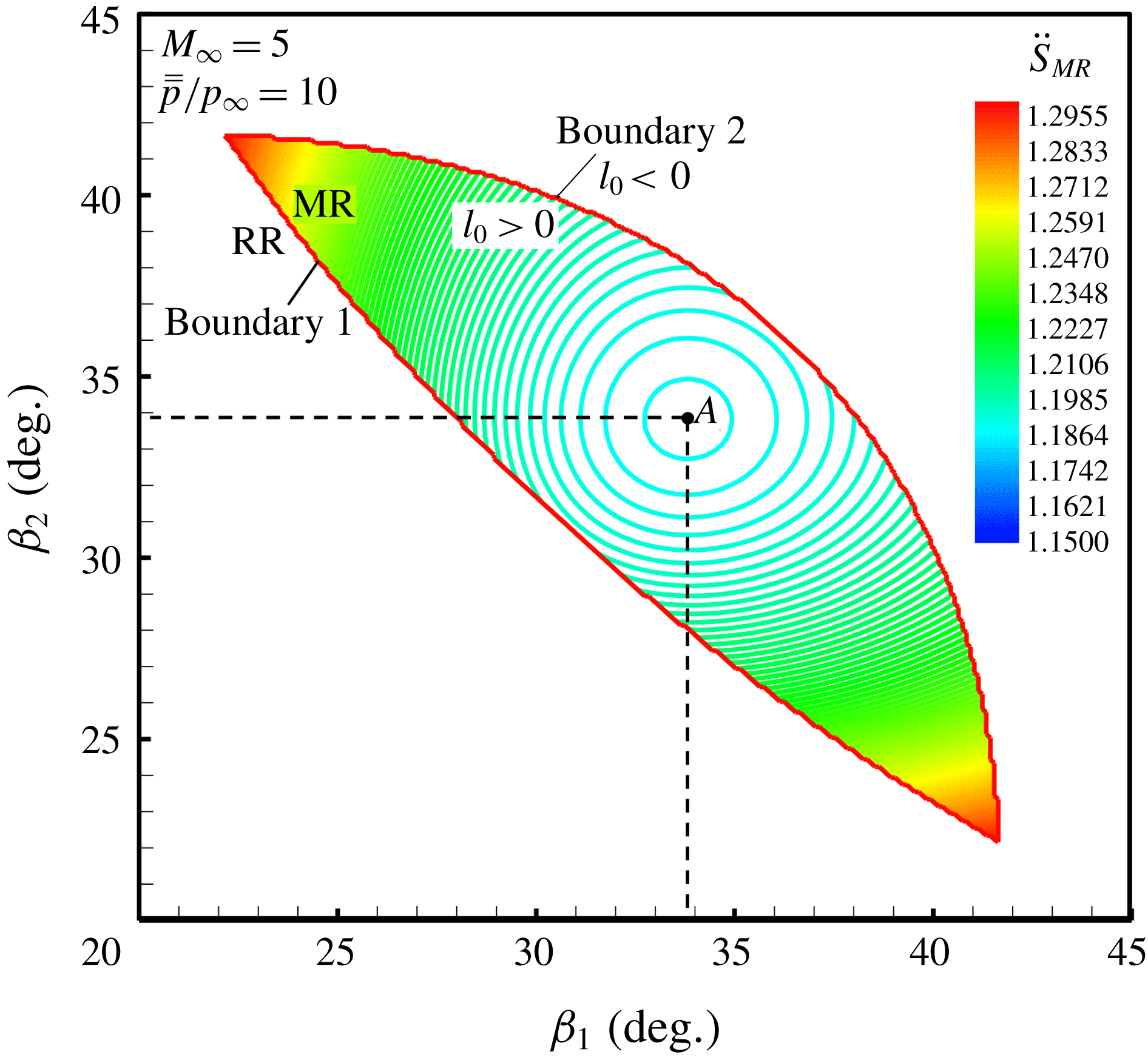
Figure 11. Contour lines of entropy production factor illustrating the relation among
 $\unicode[STIX]{x1D6FD}_{1}$
,
$\unicode[STIX]{x1D6FD}_{1}$
,
 $\unicode[STIX]{x1D6FD}_{2}$
and
$\unicode[STIX]{x1D6FD}_{2}$
and
 $\ddot{S}_{MR}$
.
$\ddot{S}_{MR}$
.
2.7 Application of the minimum entropy production principle to Mach reflection
According to (2.21), figure 11 illustrates the relation contour lines among
 $\unicode[STIX]{x1D6FD}_{1}$
,
$\unicode[STIX]{x1D6FD}_{1}$
,
 $\unicode[STIX]{x1D6FD}_{2}$
and
$\unicode[STIX]{x1D6FD}_{2}$
and
 $\ddot{S}_{MR}$
under the upstream and downstream conditions of
$\ddot{S}_{MR}$
under the upstream and downstream conditions of
 $M_{\infty }=5$
and
$M_{\infty }=5$
and
 $\overline{\overline{p}}=10$
, respectively. The boundary 1 is the lower limit that fulfills the von Neumann criterion, i.e. the existence of MR solution; boundary 2 is the upper limit that keeps
$\overline{\overline{p}}=10$
, respectively. The boundary 1 is the lower limit that fulfills the von Neumann criterion, i.e. the existence of MR solution; boundary 2 is the upper limit that keeps
 $0<l_{0}<1$
, which means that it is impossible that the length of the Mach stem will be negative or longer than the height of the entrance. The possible solutions of MR reside in the region between boundary 1 and boundary 2. Point
$0<l_{0}<1$
, which means that it is impossible that the length of the Mach stem will be negative or longer than the height of the entrance. The possible solutions of MR reside in the region between boundary 1 and boundary 2. Point
 $A$
fulfills the conditions that
$A$
fulfills the conditions that
 $$\begin{eqnarray}\left.\begin{array}{@{}c@{}}\displaystyle {\displaystyle \frac{\unicode[STIX]{x2202}^{2}f_{MR}}{\unicode[STIX]{x2202}\unicode[STIX]{x1D6FD}_{1}\unicode[STIX]{x2202}\unicode[STIX]{x1D6FD}_{2}}}=0,\\ \displaystyle {\displaystyle \frac{\unicode[STIX]{x2202}^{2}f_{MR}}{\unicode[STIX]{x2202}^{2}\unicode[STIX]{x1D6FD}_{1}}}\geqslant 0,\\ \displaystyle {\displaystyle \frac{\unicode[STIX]{x2202}^{2}f_{MR}}{\unicode[STIX]{x2202}^{2}\unicode[STIX]{x1D6FD}_{2}}}\geqslant 0.\end{array}\right\}\end{eqnarray}$$
This results in
 $\unicode[STIX]{x1D6FD}_{1}=\unicode[STIX]{x1D6FD}_{2}=33.82^{\circ }$
, which corresponds to a structure that fulfills the minimum entropy production. Hence the total entropy production of a symmetrical MR induced by separation is less than that of asymmetrical ones, which is different from that of RR under the same conditions. For further work, the solutions that fulfill the conditions of (2.22) with a steady
$\unicode[STIX]{x1D6FD}_{1}=\unicode[STIX]{x1D6FD}_{2}=33.82^{\circ }$
, which corresponds to a structure that fulfills the minimum entropy production. Hence the total entropy production of a symmetrical MR induced by separation is less than that of asymmetrical ones, which is different from that of RR under the same conditions. For further work, the solutions that fulfill the conditions of (2.22) with a steady
 $M_{\infty }=5$
and an increasing
$M_{\infty }=5$
and an increasing
 $\overline{\overline{p}}$
are calculated and illustrated in figure 12. There,
$\overline{\overline{p}}$
are calculated and illustrated in figure 12. There,
 $\overline{\overline{p}}/p_{\infty }=7.58$
and
$\overline{\overline{p}}/p_{\infty }=7.58$
and
 $\overline{\overline{p}}/p_{\infty }=29$
are the minimum and maximum downstream conditions for the existence of Mach reflection, respectively. As can be seen, the structure under different values of
$\overline{\overline{p}}/p_{\infty }=29$
are the minimum and maximum downstream conditions for the existence of Mach reflection, respectively. As can be seen, the structure under different values of
 $\overline{\overline{p}}/p_{\infty }$
that fulfills the minimum entropy production always keeps the shock angles at
$\overline{\overline{p}}/p_{\infty }$
that fulfills the minimum entropy production always keeps the shock angles at
 $\unicode[STIX]{x1D6FD}_{1}=\unicode[STIX]{x1D6FD}_{2}=33.82^{\circ }$
, and it is only characterized by an increasing Mach stem.
$\unicode[STIX]{x1D6FD}_{1}=\unicode[STIX]{x1D6FD}_{2}=33.82^{\circ }$
, and it is only characterized by an increasing Mach stem.
Since the solutions that fulfill the minimum entropy production both exist in RR and MR, there needs to be a comprehensive analysis.

Figure 12. Diagram illustrating the relation between
 $\overline{\overline{p}}$
and incident shock angles as well as Mach stem that fulfill the minimum entropy production.
$\overline{\overline{p}}$
and incident shock angles as well as Mach stem that fulfill the minimum entropy production.
2.8 Comprehensive analysis in RR and MR induced by separation
The methods mentioned above establish the connection among upstream flow, shock configurations and downstream flow in separation-induced RR and MR, respectively. To compare the characteristics of minimum entropy production between RR and MR, the entropy production factors as well as flow deflection angles that fulfill the minimum entropy production are calculated and illustrated together in figure 13. There,
 $\ddot{S}_{RR}$
and
$\ddot{S}_{RR}$
and
 $\ddot{S}_{MR}$
are the minimum entropy production factors of RR and MR, respectively;
$\ddot{S}_{MR}$
are the minimum entropy production factors of RR and MR, respectively;
 $\unicode[STIX]{x1D6FC}_{RR1}$
and
$\unicode[STIX]{x1D6FC}_{RR1}$
and
 $\unicode[STIX]{x1D6FC}_{RR2}$
are the flow deflection angles of RR on the top and bottom, respectively;
$\unicode[STIX]{x1D6FC}_{RR2}$
are the flow deflection angles of RR on the top and bottom, respectively;
 $\unicode[STIX]{x1D6FC}_{MR}$
is the flow deflection angle of MR on the top or bottom (they are a same angle); and
$\unicode[STIX]{x1D6FC}_{MR}$
is the flow deflection angle of MR on the top or bottom (they are a same angle); and
 $\unicode[STIX]{x1D6FC}^{vN}$
and
$\unicode[STIX]{x1D6FC}^{vN}$
and
 $\unicode[STIX]{x1D6FC}^{D}$
are the von Neumann condition and detachment condition, respectively. As indicated in figure 13, seven typical positions are marked from (i) to (vii) and explained as follows:
$\unicode[STIX]{x1D6FC}^{D}$
are the von Neumann condition and detachment condition, respectively. As indicated in figure 13, seven typical positions are marked from (i) to (vii) and explained as follows:
(i)
$\overline{\overline{p}}/p_{\infty }=1$
is the minimum downstream condition for the existence of shock reflection solutions;(ii)
$\overline{\overline{p}}/p_{\infty }=4.46$
is the minimum downstream condition for the existence of asymmetrical RR solutions;(iii)
$\overline{\overline{p}}/p_{\infty }=7.58$
is the minimum downstream condition for the existence of MR solutions;(iv)
$\overline{\overline{p}}/p_{\infty }=13.05$
is a critical downstream condition for the possibility of RR–MR transition;(v)
$\overline{\overline{p}}/p_{\infty }=18.39$
is another critical downstream condition for the possibility of RR–MR transition;(vi)
$\overline{\overline{p}}/p_{\infty }=22.49$
is the maximum downstream condition for the existence of RR solutions;(vii)
$\overline{\overline{p}}/p_{\infty }=29$
is the maximum downstream condition for the existence of MR solutions.


It can be seen from the typical positions that the entropy production factor of MR is lower than that of RR during the overlapping stage, i.e.
 $\ddot{S}_{MR}<\ddot{S}_{RR}$
when
$\ddot{S}_{MR}<\ddot{S}_{RR}$
when
 $7.58<\overline{\overline{p}}/p_{\infty }<22.49$
. However, RR cannot transfer to MR until
$7.58<\overline{\overline{p}}/p_{\infty }<22.49$
. However, RR cannot transfer to MR until
 $\unicode[STIX]{x1D6FC}_{RR2}$
reaches the von Neumann condition, i.e.
$\unicode[STIX]{x1D6FC}_{RR2}$
reaches the von Neumann condition, i.e.
 $\unicode[STIX]{x1D6FC}_{RR2}\geqslant \unicode[STIX]{x1D6FC}^{vN}$
when
$\unicode[STIX]{x1D6FC}_{RR2}\geqslant \unicode[STIX]{x1D6FC}^{vN}$
when
 $13.05\leqslant \overline{\overline{p}}/p_{\infty }\leqslant 18.39$
(figure 13
b), which means
$13.05\leqslant \overline{\overline{p}}/p_{\infty }\leqslant 18.39$
(figure 13
b), which means
 $\overline{\overline{p}}/p_{\infty }=13.05$
is a criterion of downstream condition for RR–MR transition. It is more complicated during
$\overline{\overline{p}}/p_{\infty }=13.05$
is a criterion of downstream condition for RR–MR transition. It is more complicated during
 $18.39\leqslant \overline{\overline{p}}/p_{\infty }\leqslant 22.49$
, as shown in figure 13(b). There, the solutions that fulfill the minimum entropy production can reside in overall RR as well as overall MR, depending on the former structure: if the former structure reaches von Neumann condition, then the current structure will be MR; if not, it will be RR, which means the structure is unsteady during this condition stage.
$18.39\leqslant \overline{\overline{p}}/p_{\infty }\leqslant 22.49$
, as shown in figure 13(b). There, the solutions that fulfill the minimum entropy production can reside in overall RR as well as overall MR, depending on the former structure: if the former structure reaches von Neumann condition, then the current structure will be MR; if not, it will be RR, which means the structure is unsteady during this condition stage.

Figure 13. Diagrams illustrating the relations between
 $\overline{\overline{p}}$
and entropy production factors as well as flow deflection angles in RR and MR that fulfill the minimum entropy production: (a) whole diagram, and (b) detailed diagram for
$\overline{\overline{p}}$
and entropy production factors as well as flow deflection angles in RR and MR that fulfill the minimum entropy production: (a) whole diagram, and (b) detailed diagram for
 $12\leqslant \overline{\overline{p}}/p_{\infty }\leqslant 23$
.
$12\leqslant \overline{\overline{p}}/p_{\infty }\leqslant 23$
.
Base on the comprehensive analysis above, the relation between
 $\overline{\overline{p}}$
and shock reflection configurations induced by separation is illustrated in figure 14. There,
$\overline{\overline{p}}$
and shock reflection configurations induced by separation is illustrated in figure 14. There,
 $RR_{S}$
and
$RR_{S}$
and
 $RR_{AS}$
denote symmetrical and asymmetrical RR, respectively;
$RR_{AS}$
denote symmetrical and asymmetrical RR, respectively;
 $MR_{S}$
is symmetrical MR;
$MR_{S}$
is symmetrical MR;
 $\unicode[STIX]{x1D6FD}_{1}$
and
$\unicode[STIX]{x1D6FD}_{1}$
and
 $\unicode[STIX]{x1D6FD}_{2}$
are the incident shock angles of RR induced by separation on the top and bottom, respectively (
$\unicode[STIX]{x1D6FD}_{2}$
are the incident shock angles of RR induced by separation on the top and bottom, respectively (
 $\unicode[STIX]{x1D6FD}_{1}$
and
$\unicode[STIX]{x1D6FD}_{1}$
and
 $\unicode[STIX]{x1D6FD}_{2}$
are interchangeable);
$\unicode[STIX]{x1D6FD}_{2}$
are interchangeable);
 $\unicode[STIX]{x1D6FD}_{0}$
is the shock angle of MR induced by separation (the angles on the top and bottom are the same); and
$\unicode[STIX]{x1D6FD}_{0}$
is the shock angle of MR induced by separation (the angles on the top and bottom are the same); and
 $l_{0}$
is the ratio of the Mach stem length to the entrance height. The critical solution of RR–MR transition is
$l_{0}$
is the ratio of the Mach stem length to the entrance height. The critical solution of RR–MR transition is
 $\unicode[STIX]{x1D6FD}_{1}=19^{\circ }$
,
$\unicode[STIX]{x1D6FD}_{1}=19^{\circ }$
,
 $\unicode[STIX]{x1D6FD}_{2}=48^{\circ }$
(or
$\unicode[STIX]{x1D6FD}_{2}=48^{\circ }$
(or
 $\unicode[STIX]{x1D6FD}_{1}=48^{\circ }$
,
$\unicode[STIX]{x1D6FD}_{1}=48^{\circ }$
,
 $\unicode[STIX]{x1D6FD}_{2}=19^{\circ }$
), which will be verified by experimental results in the following sections.
$\unicode[STIX]{x1D6FD}_{2}=19^{\circ }$
), which will be verified by experimental results in the following sections.

Figure 14. Diagram illustrating the relation between
 $\overline{\overline{p}}$
and shock reflection configurations that fulfill the minimum entropy production.
$\overline{\overline{p}}$
and shock reflection configurations that fulfill the minimum entropy production.
3 Experimental results and discussions
3.1 Experimental apparatus and test model
The experiment was conducted in a hypersonic wind tunnel; previous research in this facility has been described in detail by Wang et al. (Reference Wang, Xue and Tian2017). There are some improved parts in the current test, as shown in figure 15. Firstly, a plug device driven by a stepper motor, which can generate a linearly increasing throttling (see Xue et al.
Reference Xue, Wang and Cheng2018), was employed to guide the downstream pressure disturbance. Secondly, 16 Kulite XTEL-190M fast-response transducers, which were operated at a rate of 10 kHz using data acquisition cards and a 10 s sampling time, were mounted along the central lines of ramps on the top and bottom, respectively. Lastly, a NAC (NAC Image Technology) Hotshot High Speed Camera, which operated at a frame rate of 5 kHz with a 6 s sampling time and a resolution of
 $608\times 436$
pixels, was used to capture the evolution of the shock reflection configuration. Table 1 shows the test conditions. A non-dimensional variable
$608\times 436$
pixels, was used to capture the evolution of the shock reflection configuration. Table 1 shows the test conditions. A non-dimensional variable
 $\unicode[STIX]{x1D6E5}$
is defined to measure the downstream throttling:
$\unicode[STIX]{x1D6E5}$
is defined to measure the downstream throttling:
 $$\begin{eqnarray}\left.\begin{array}{@{}c@{}}\unicode[STIX]{x1D6E5}=\left(1-\displaystyle {\displaystyle \frac{A_{tx}}{A_{0}}}\right)\times 100\,\%,\\ A_{tx}=2bx\sin 20^{\circ },\end{array}\right\}\end{eqnarray}$$
where
 $A_{tx}$
denotes the area size that can flow across the outlet effectively, and
$A_{tx}$
denotes the area size that can flow across the outlet effectively, and
 $A_{0}$
is the total area of the outlet.
$A_{0}$
is the total area of the outlet.

Figure 15. Schematic of the test model and downstream throttling device (Wang et al. Reference Wang, Xue and Tian2017; Xue et al. Reference Xue, Wang and Cheng2018).
Table 1. Test conditions.

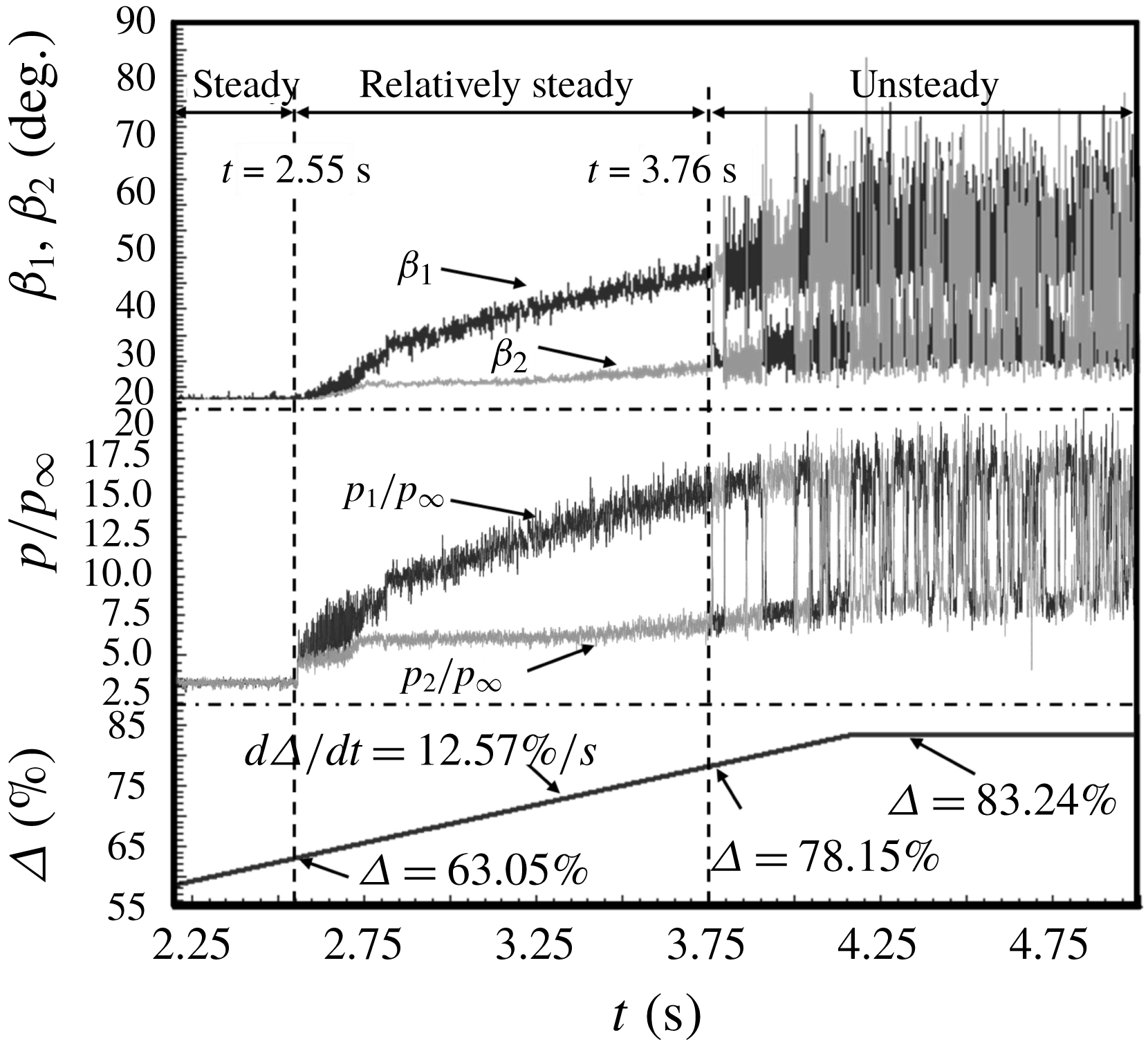
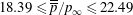
Figure 16. Time histories of incident shock angles (
 $\unicode[STIX]{x1D6FD}_{1}$
,
$\unicode[STIX]{x1D6FD}_{1}$
,
 $\unicode[STIX]{x1D6FD}_{2}$
), dynamic wall pressures (
$\unicode[STIX]{x1D6FD}_{2}$
), dynamic wall pressures (
 $p_{1}$
,
$p_{1}$
,
 $p_{2}$
), and downstream throttling degree (
$p_{2}$
), and downstream throttling degree (
 $\unicode[STIX]{x1D6E5}$
).
$\unicode[STIX]{x1D6E5}$
).
3.2 Time history characteristics of incident shock angles and wall pressures
A quantization method of schlieren images based on a grey-level matrix (see Xue et al.
Reference Xue, Wang and Cheng2018) was employed to analyse the dynamic characteristics of the shock configuration, and the time history of shock angles was detected. The experimental results are illustrated in figure 16. In figure 16,
 $\unicode[STIX]{x1D6FD}_{1}$
and
$\unicode[STIX]{x1D6FD}_{1}$
and
 $\unicode[STIX]{x1D6FD}_{2}$
are the incident shock angles induced by separation on the top and bottom, respectively;
$\unicode[STIX]{x1D6FD}_{2}$
are the incident shock angles induced by separation on the top and bottom, respectively;
 $p_{1}$
and
$p_{1}$
and
 $p_{2}$
are the dynamic wall pressures obtained by transducers T
$p_{2}$
are the dynamic wall pressures obtained by transducers T
 $_{1}$
and B
$_{1}$
and B
 $_{1}$
(locations in figure 15), which are the most upstream transducers behind incident shocks on the top and bottom, respectively; and
$_{1}$
(locations in figure 15), which are the most upstream transducers behind incident shocks on the top and bottom, respectively; and
 $\unicode[STIX]{x1D6E5}$
is the downstream throttling degree. Figure 17 shows the standard deviation analysis for illustrating the fluctuation amplitude of
$\unicode[STIX]{x1D6E5}$
is the downstream throttling degree. Figure 17 shows the standard deviation analysis for illustrating the fluctuation amplitude of
 $p_{1}$
,
$p_{1}$
,
 $p_{2}$
and
$p_{2}$
and
 $\overline{\overline{p}}$
, in which
$\overline{\overline{p}}$
, in which
 $\overline{\overline{p}}$
is produced by using
$\overline{\overline{p}}$
is produced by using
 $\unicode[STIX]{x1D6FD}_{1}$
,
$\unicode[STIX]{x1D6FD}_{1}$
,
 $\unicode[STIX]{x1D6FD}_{2}$
,
$\unicode[STIX]{x1D6FD}_{2}$
,
 $p_{1}$
and
$p_{1}$
and
 $p_{2}$
according to the definition of
$p_{2}$
according to the definition of
 $\overline{\overline{p}}$
. Figure 18 shows details of upstream and downstream dynamic pressures as well as
$\overline{\overline{p}}$
. Figure 18 shows details of upstream and downstream dynamic pressures as well as
 $\overline{\overline{p}}$
covering the transition process. Figure 19 shows wall pressure distributions and the accompanying schlieren images during the transition process. As can be indicated, the wall pressures and shock angles were steady with
$\overline{\overline{p}}$
covering the transition process. Figure 19 shows wall pressure distributions and the accompanying schlieren images during the transition process. As can be indicated, the wall pressures and shock angles were steady with
 $\unicode[STIX]{x1D6E5}$
increasing linearly before the appearance of a separation region (figure 16,
$\unicode[STIX]{x1D6E5}$
increasing linearly before the appearance of a separation region (figure 16,
 $t=2.55$
s,
$t=2.55$
s,
 $\unicode[STIX]{x1D6E5}=63.05\,\%$
); the shock configuration can be regarded as a relatively steady flow before the RR–MR transition, while it is unsteady after the transition (figure 16,
$\unicode[STIX]{x1D6E5}=63.05\,\%$
); the shock configuration can be regarded as a relatively steady flow before the RR–MR transition, while it is unsteady after the transition (figure 16,
 $t=3.76$
s,
$t=3.76$
s,
 $\unicode[STIX]{x1D6E5}=78.15\,\%$
). During the RR–MR transition process, downstream pressures turned out to be more stable and symmetrical than upstream ones (figure 19). Although
$\unicode[STIX]{x1D6E5}=78.15\,\%$
). During the RR–MR transition process, downstream pressures turned out to be more stable and symmetrical than upstream ones (figure 19). Although
 $p_{1}$
and
$p_{1}$
and
 $p_{2}$
experienced a sharp change in amplitude,
$p_{2}$
experienced a sharp change in amplitude,
 $\overline{\overline{p}}$
was more stable (figure 17,
$\overline{\overline{p}}$
was more stable (figure 17,
 $t=3.76$
s,
$t=3.76$
s,
 $\unicode[STIX]{x1D6E5}=78.15\,\%$
), which was similar to downstream pressures (figure 18, T
$\unicode[STIX]{x1D6E5}=78.15\,\%$
), which was similar to downstream pressures (figure 18, T
 $_{8}$
and B
$_{8}$
and B
 $_{8}$
).
$_{8}$
).
Figure 17. Standard deviation analysis of dynamic pressure signals (
 $p_{1}$
,
$p_{1}$
,
 $p_{2}$
and
$p_{2}$
and
 $\overline{\overline{p}}$
) for illustrating the amplitude of pressure fluctuation.
$\overline{\overline{p}}$
) for illustrating the amplitude of pressure fluctuation.

Figure 18. Dynamic wall pressures for illustrating shock reflection transition.
The separation-induced shock reflection is mainly generated by downstream pressure disturbance, while the asymmetrical flow configurations as well as transition only exist in the upstream flow field. According to current theory, the estimation of downstream high back-pressure plays an important role in the minimum entropy production principle. However, downstream pressures are hardly connected to upstream flow structures due to the long flow path. Comparing figures 16–19, it is clear that
 $\overline{\overline{p}}$
is suitable to measure the effect of downstream pressure disturbance. On the one hand, the transition of flow configuration is characterized by the sharp change of upstream wall pressures, while it exerts less influence on downstream wall pressures, which is the same as
$\overline{\overline{p}}$
is suitable to measure the effect of downstream pressure disturbance. On the one hand, the transition of flow configuration is characterized by the sharp change of upstream wall pressures, while it exerts less influence on downstream wall pressures, which is the same as
 $\overline{\overline{p}}$
(figures 18 and 19). On the other hand, the original flow disturbance is generated by downstream flow choking measured by
$\overline{\overline{p}}$
(figures 18 and 19). On the other hand, the original flow disturbance is generated by downstream flow choking measured by
 $\unicode[STIX]{x1D6E5}$
, and the positive correlation between
$\unicode[STIX]{x1D6E5}$
, and the positive correlation between
 $\unicode[STIX]{x1D6E5}$
and
$\unicode[STIX]{x1D6E5}$
and
 $\overline{\overline{p}}$
is distinct (figures 16 and 17). Therefore,
$\overline{\overline{p}}$
is distinct (figures 16 and 17). Therefore,
 $\overline{\overline{p}}$
changes along with the downstream flow condition and would not be altered by upstream flow configurations, and it is the same with downstream pressures, which means
$\overline{\overline{p}}$
changes along with the downstream flow condition and would not be altered by upstream flow configurations, and it is the same with downstream pressures, which means
 $\overline{\overline{p}}$
could represent back-pressure. Because
$\overline{\overline{p}}$
could represent back-pressure. Because
 $\overline{\overline{p}}$
can be estimated by upstream wall pressures and incident shock angles on the top and bottom, respectively, it can be used as the critical parameter of flow configuration.
$\overline{\overline{p}}$
can be estimated by upstream wall pressures and incident shock angles on the top and bottom, respectively, it can be used as the critical parameter of flow configuration.

Figure 19. Wall-pressure distributions and flow configurations for illustrating shock reflection transition.

Figure 20. The evolution processes of shock configuration transition: (a) symmetrical RR to asymmetrical RR, and (b) asymmetrical RR to symmetrical MR.
3.3 Evolution processes of shock configuration
The evolution processes of symmetrical RR to asymmetrical RR transition and asymmetrical RR to symmetrical MR transition are illustrated in figures 20(a) and 20(b), respectively. As can be seen in figure 20(a), the incident shock angle on the top increased smoothly, while it changed indistinctly on the bottom, which demonstrates a gradual transition in symmetrical RR to asymmetrical RR. However, in figure 20(b), the process lasted no more than 4 ms from asymmetrical RR to symmetrical MR with a sharp change in
 $\unicode[STIX]{x1D6FD}_{1}=48^{\circ }$
and
$\unicode[STIX]{x1D6FD}_{1}=48^{\circ }$
and
 $\unicode[STIX]{x1D6FD}_{2}=19^{\circ }$
to
$\unicode[STIX]{x1D6FD}_{2}=19^{\circ }$
to
 $\unicode[STIX]{x1D6FD}_{1}=\unicode[STIX]{x1D6FD}_{2}=34^{\circ }$
. Then the configuration turned back to asymmetrical RR immediately, and the subsequent process is asymmetrical RR to symmetrical MR again.
$\unicode[STIX]{x1D6FD}_{1}=\unicode[STIX]{x1D6FD}_{2}=34^{\circ }$
. Then the configuration turned back to asymmetrical RR immediately, and the subsequent process is asymmetrical RR to symmetrical MR again.
The evolution processes demonstrate that it is a relatively steady flow in RR while it is unsteady when RR–MR transition occurs, which is the same as the analysis from dynamic transducer signals. Figure 21 gives the statistical results of incident shock angles including 6000 schlieren images. Figure 22 indicates that the incident shock angles of symmetrical MR under different
 $\overline{\overline{p}}$
can keep the same degree (
$\overline{\overline{p}}$
can keep the same degree (
 $\unicode[STIX]{x1D6FD}_{1}=\unicode[STIX]{x1D6FD}_{2}=34^{\circ }$
) with an increasing Mach stem (it may be regarded as a normal shock when
$\unicode[STIX]{x1D6FD}_{1}=\unicode[STIX]{x1D6FD}_{2}=34^{\circ }$
) with an increasing Mach stem (it may be regarded as a normal shock when
 $\overline{\overline{p}}/p_{\infty }=29$
and
$\overline{\overline{p}}/p_{\infty }=29$
and
 $l_{0}=1$
). The results above demonstrate a good agreement between theory and experiment.
$l_{0}=1$
). The results above demonstrate a good agreement between theory and experiment.

Figure 21. Statistical results of incident shock angles detected from schlieren images: (a) RR, and (b) MR.

Figure 22. Typical MR configurations under the different downstream conditions of
 $\overline{\overline{p}}$
.
$\overline{\overline{p}}$
.
3.4 Solution path of reflected shock that fulfills the minimum entropy production

Figure 23. Typical (a) shock configurations and (b) reflected shock solutions under different downstream conditions.

Figure 24. The reflected shock solution path that fulfills the minimum entropy production.
The schlieren images under different
 $\overline{\overline{p}}$
are selected to illustrate the typical shock configurations, which are shown in figure 23(a), and the accompanying reflected shock solutions,
$\overline{\overline{p}}$
are selected to illustrate the typical shock configurations, which are shown in figure 23(a), and the accompanying reflected shock solutions,
 $a$
–
$a$
–
 $i$
, are depicted via shock polar lines in figure 23(b). It is obvious that there is a solution path in the overall RR domain, along which the reflected shock solutions fulfill the minimum entropy production. Based on the comprehensive analysis of theoretical and experimental results, the path is depicted clearly in figure 24, in which the direction means a rising influence of the downstream condition. The path is along a symmetry line at first, then it divides into two opposite paths at the differentiation point, which means the symmetrical configuration fulfills the minimum entropy production with weak enough influence of downstream condition, while it may change to be asymmetrical when the downstream condition increases to a critical level, and the direction chosen by flow is random (as shown in figure 20
a). When the two divided paths reach the strong polar line of the incident shock at the transition points, the configuration will transform from RR to MR (as shown in figure 20
b). In fact, when the downstream condition approaches the transition point in the experiment, the RR–MR transition and MR–RR transition will occur repeatedly. The most plausible explanation is that the pressures of the solutions along the dashed path line are too close, and the solutions during the transition process reside on the dashed path line, which means a small downstream pressure disturbance may cause a sharp change in shock structure. Hence, it is confirmed that the solutions on the solid path lines can be regarded as relatively steady, while the solutions on the dashed path lines are unsteady. Note that the path is produced by the flow itself, which means the flow chooses a way to ensure the solutions fulfill the minimum entropy production under different downstream conditions. Therefore, the solution path can be used to determine the steadiest shock reflection, according to various condition requirements.
$i$
, are depicted via shock polar lines in figure 23(b). It is obvious that there is a solution path in the overall RR domain, along which the reflected shock solutions fulfill the minimum entropy production. Based on the comprehensive analysis of theoretical and experimental results, the path is depicted clearly in figure 24, in which the direction means a rising influence of the downstream condition. The path is along a symmetry line at first, then it divides into two opposite paths at the differentiation point, which means the symmetrical configuration fulfills the minimum entropy production with weak enough influence of downstream condition, while it may change to be asymmetrical when the downstream condition increases to a critical level, and the direction chosen by flow is random (as shown in figure 20
a). When the two divided paths reach the strong polar line of the incident shock at the transition points, the configuration will transform from RR to MR (as shown in figure 20
b). In fact, when the downstream condition approaches the transition point in the experiment, the RR–MR transition and MR–RR transition will occur repeatedly. The most plausible explanation is that the pressures of the solutions along the dashed path line are too close, and the solutions during the transition process reside on the dashed path line, which means a small downstream pressure disturbance may cause a sharp change in shock structure. Hence, it is confirmed that the solutions on the solid path lines can be regarded as relatively steady, while the solutions on the dashed path lines are unsteady. Note that the path is produced by the flow itself, which means the flow chooses a way to ensure the solutions fulfill the minimum entropy production under different downstream conditions. Therefore, the solution path can be used to determine the steadiest shock reflection, according to various condition requirements.
4 Conclusions
In the current study, the shock reflection configurations induced by separation are studied theoretically and experimentally. A symmetrical test model with two ramps of
 $7^{\circ }$
is tested in a free-stream flow of Mach number 5, and a downstream throttling device is used to generate the separation region on ramps. The minimum entropy production principle is employed to analyse the shock configurations as well as RR–MR transition. In addition, a variable, represented as
$7^{\circ }$
is tested in a free-stream flow of Mach number 5, and a downstream throttling device is used to generate the separation region on ramps. The minimum entropy production principle is employed to analyse the shock configurations as well as RR–MR transition. In addition, a variable, represented as
 $\overline{\overline{p}}$
, is proposed to measure the influence of downstream pressure disturbance, based on which the following conclusions are obtained.
$\overline{\overline{p}}$
, is proposed to measure the influence of downstream pressure disturbance, based on which the following conclusions are obtained.
The relation among upstream and downstream conditions and shock configurations as well as total entropy production is established by an analytical model. Moreover, separation-induced incident shock angles may be determined by solutions that fulfill the minimum entropy production, and the criterion of RR–MR transition is successfully predicted, which indicate a good agreement with experimental results.
On the other hand, there is a solution path residing in the overall RR domain and the strong incident shock polar line, along which the reflected shock solutions fulfill the minimum entropy production. Furthermore, the shock configuration is relatively steady before the path reaches the strong incident shock polar line, while it is unsteady after that. Therefore, the solution path is very helpful to determine incident shock angles that may induce the steadiest shock configurations in separation-induced flows.
Acknowledgements
This work was supported by the National Natural Science Foundation of China (51776096 and 51476076), and a project funded by the Priority Academic Program Development of Jiangsu Higher Education Institutions (PAPD 016001). This support is gratefully acknowledged.


