2.1 Initial conditions

Direct numerical simulations of an $M_{c}=1.1$ compressible mixing layer are performed for a PG and for a (BZT) DG. In the first case, air is chosen and considered as a PG as done by Freund et al. (Reference Freund, Lele and Moin2000). For the DG simulations, perfluorotripentylamine (FC-70, C$_{15}$F$_{33}$N) is used. It is the same DG used by Fergason et al. (Reference Fergason, Ho, Argrow and Emanuel2001) in order to simulate rarefaction shock waves in a shock tube. It is in particular used as heat transfer fluid, is almost non-toxic and has been evaluated as synthetic blood (Costello, Flynn & Owens Reference Costello, Flynn and Owens2000). Physical parameters useful for the thermodynamic description of FC-70 are given in table 1, as taken from Cramer (Reference Cramer1989).

Table 1. Physical parameters of FC-70 (Cramer Reference Cramer1989). The critical pressure $p_{c}$, the critical temperature $T_{c}$, the boiling temperature $T_{b}$ and the compressibility factor $Z_{c}=p_{c}v_{c}/(RT_{c})$ are the input data for the MH equation. The critical specific volume $v_{c}$ is deduced from the aforementioned parameters. The acentric factor $n$ and the $c_{v}(T_{c})/R$ ratio are used to compute the heat capacity $c_{v}(T)$ ($R={\mathcal{R}}/M$ being the specific gas constant computed from the universal gas constant ${\mathcal{R}}$ with $M$ being the molar mass of the gas).

The initial conditions of the mixing layer require the choice of the initial operating thermodynamic point in the $p$–$v$ diagram. As described in figure 1, this initial state is chosen within the inversion zone of FC-70 in order to favour the occurrence of expansion shocklets and to maximize DG effects on turbulence. This is also in that region that compressibility effects are the largest since the sound speed is reduced (Colonna & Guardone Reference Colonna and Guardone2006), which maximizes the Mach number. Figure 1 also shows the adiabatic curve on which the initial operating point is lying in the non-dimensional $p$–$v$ diagram. The corresponding initial value of the fundamental derivative of gas dynamics is $\unicode[STIX]{x1D6E4}_{initial}=-0.284$. During the development of the mixing layer, the thermodynamic conditions stay within a close range around the adiabatic curve as shown in figure 1, because shocklet entropy losses and mechanical dissipation are weak in our case. Also, almost all the thermodynamic states stay within the inversion zone throughout the DG simulation. For air, the same values of reduced specific volume and reduced pressure are selected for the initial thermodynamic state. Critical values used for air are the critical pressure $p_{c}=3.7663\times 10^{6}~\text{Pa}$ and the specific volume $v_{c}=3.13\times 10^{-3}~\text{m}^{3}~\text{kg}^{-1}$ (Stephan & Laesecke Reference Stephan and Laesecke1985).

Table 2. Simulation parameters. Lengths $L_{x}$, $L_{y}$ and $L_{z}$ denote computational domain lengths measured in terms of initial momentum thickness and $N_{x}$, $N_{y}$ and $N_{z}$ denote the number of grid points. All grids are uniform.

a Referred to as the $16.8M$ simulation, where $16.8M$ corresponds to the number of grid cells.

b Referred to as the $134M$ simulation, where $134M$ corresponds to the number of grid cells.

The main non-dimensional characteristics of the compressible mixing layer are the convective Mach number (1.3) and the Reynolds number based on the initial momentum thickness $\unicode[STIX]{x1D6FF}_{\unicode[STIX]{x1D703},0}$:

(2.1)$$\begin{eqnarray}Re_{\unicode[STIX]{x1D6FF}_{\unicode[STIX]{x1D703},0}}=\unicode[STIX]{x0394}u\unicode[STIX]{x1D6FF}_{\unicode[STIX]{x1D703},0}/\unicode[STIX]{x1D708},\end{eqnarray}$$

where $\unicode[STIX]{x1D708}$ denotes the kinematic viscosity and the momentum thickness at time $t$ is defined as

(2.2)$$\begin{eqnarray}\unicode[STIX]{x1D6FF}_{\unicode[STIX]{x1D703}}(t)=\frac{1}{\unicode[STIX]{x1D70C}_{0}\unicode[STIX]{x0394}u^{2}}\int _{-\infty }^{+\infty }\overline{\unicode[STIX]{x1D70C}}\left(\frac{\unicode[STIX]{x0394}u^{2}}{4}-\tilde{u} _{x}^{2}\right)\text{d}y,\end{eqnarray}$$

with $\unicode[STIX]{x1D70C}_{0}=(\unicode[STIX]{x1D70C}_{1}+\unicode[STIX]{x1D70C}_{2})/2$ the averaged density and $\tilde{u} _{x}$ the Favre averaged streamwise velocity (defined in (2.13)).

The first part of the study aims at validating the present DNS results using the results of Pantano & Sarkar (Reference Pantano and Sarkar2002) as reference. Following this reference work, the convective Mach number is set equal to 1.1 as previously mentioned, the initial density ratio between the upper and lower streams is equal to unity and the Reynolds number based on the initial momentum thickness is set equal to 160. Table 2 reports the simulation parameters (domain size, grid resolution, dimensional values of velocity and initial momentum thickness). The ratio $r$ between the Kolmogorov scale and the cell size is about 0.52 for the least refined mesh ($16.8M$ simulation) during the selected self-similar range (see § 3.1). To check grid convergence and because the value $r=0.52$ corresponding to the baseline mesh is not very large for a DNS, a second DNS has been performed with a refined mesh obtained by doubling the number of grid cells in each direction ($134M$ simulation) yielding a ratio $r$ equal to 1.03. Turbulent scales are adequately resolved since the TKE is very low close to the Kolmogorov scale (Moin & Mahesh Reference Moin and Mahesh1998).

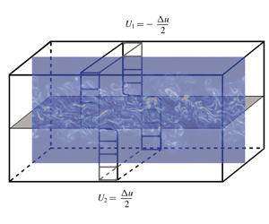
Figure 2. Schematic view of the temporal mixing layer configuration. The grey plane represents the initial momentum thickness and its thickness is at scale with the lengths of the computational domain.

In the present study, the temporal mixing layer, less computationally expensive, is chosen instead of the spatial mixing layer. There are slight differences between the two configurations. For the temporal mixing layer, the two streams flow in opposite directions, which enables one to increase the differential speed with a less important absolute speed for each stream (see figure 2). For the spatial mixing layer, both streams flow in the same direction and a speed gap which corresponds to the differential speed is imposed. The transition from one configuration to the other is a change of Galilean reference frame given by (de Bruin Reference de Bruin2001)

(2.3)$$\begin{eqnarray}t\unicode[STIX]{x0394}u_{temporal}=\frac{x\unicode[STIX]{x0394}u_{spatial}}{u_{c}},\end{eqnarray}$$

where $t$ denotes the time scale of the temporal configuration, $\unicode[STIX]{x0394}u_{temporal}$ the differential speed of the temporal evolution, $\unicode[STIX]{x0394}u_{spatial}$ the differential speed of the spatial evolution, $u_{c}=(U_{1}+U_{2})/2$ the convective speed and $x$ the streamwise position scale of the spatial configuration.

The temporal mixing layer requires periodic boundary conditions in the $x$ and $z$ directions. A non-reflective boundary condition is imposed in the $y$ direction to prevent the reflection of acoustic waves inside the computational domain. The NSCBC model proposed by Poinsot & Lele (Reference Poinsot and Lele1992) is used.

The mean streamwise velocity is initialized with a hyperbolic tangent profile:

(2.4)$$\begin{eqnarray}\bar{u}_{x}(y)=\frac{\unicode[STIX]{x0394}u}{2}\tanh \left(-\frac{y}{2\unicode[STIX]{x1D6FF}_{\unicode[STIX]{x1D703},0}}\right).\end{eqnarray}$$

The complete streamwise velocity field is obtained by adding a fluctuating component to the mean component. For the $y$ and $z$ components of the velocity, the mean part is set equal to zero. A Passot–Pouquet spectrum is imposed for the initial velocity fluctuation:

(2.5)$$\begin{eqnarray}E(k)=(k/k_{0})^{4}\exp (-2(k/k_{0})^{2}),\end{eqnarray}$$

where $k$ denotes the wavenumber. The peak wavenumber $k_{0}$ corresponds to the integral scale for which the TKE is maximum inside the initial mixing layer. Peak wavenumber $k_{0}$ is set to $2\unicode[STIX]{x03C0}/(L_{x}/48)$. The obtained velocity field is then multiplied by an exponential decay over the $y$ direction in order to inject turbulent energy in the initial momentum thickness only. That is done in the same way as Pantano & Sarkar (Reference Pantano and Sarkar2002):

(2.6)$$\begin{eqnarray}f(y)=\frac{1}{\unicode[STIX]{x1D70E}\sqrt{2\unicode[STIX]{x03C0}}}\exp \left(-\frac{(y-L_{y}/2)^{2}}{2\unicode[STIX]{x1D70E}^{2}}\right),\end{eqnarray}$$

where the full width at half maximum of the peak is set equal to the initial momentum thickness $\unicode[STIX]{x1D6FF}_{\unicode[STIX]{x1D703},0}=2\unicode[STIX]{x1D70E}\sqrt{2\ln (2)}$. Also, the Gaussian distribution is normalized to reach a maximum value of 1 at the centre $y=L_{y}/2$.

2.2 Governing equations

The unsteady, three-dimensional, compressible Navier–Stokes equations are solved to describe the temporally evolving mixing layer:

(2.7)$$\begin{eqnarray}\displaystyle & \displaystyle \frac{\unicode[STIX]{x2202}\unicode[STIX]{x1D70C}}{\unicode[STIX]{x2202}t}+\frac{\unicode[STIX]{x2202}(\unicode[STIX]{x1D70C}u_{i})}{\unicode[STIX]{x2202}x_{i}}=0, & \displaystyle\end{eqnarray}$$

(2.8)$$\begin{eqnarray}\displaystyle & \displaystyle \frac{\unicode[STIX]{x2202}(\unicode[STIX]{x1D70C}u_{i})}{\unicode[STIX]{x2202}t}+\frac{\unicode[STIX]{x2202}(\unicode[STIX]{x1D70C}u_{i}u_{j})}{\unicode[STIX]{x2202}x_{j}}=-\frac{\unicode[STIX]{x2202}p}{\unicode[STIX]{x2202}x_{i}}+\frac{\unicode[STIX]{x2202}\unicode[STIX]{x1D70F}_{ij}}{\unicode[STIX]{x2202}x_{j}}, & \displaystyle\end{eqnarray}$$

(2.9)$$\begin{eqnarray}\displaystyle & \displaystyle \frac{\unicode[STIX]{x2202}(\unicode[STIX]{x1D70C}E)}{\unicode[STIX]{x2202}t}+\frac{\unicode[STIX]{x2202}[(\unicode[STIX]{x1D70C}E+p)u_{j}]}{\unicode[STIX]{x2202}x_{j}}=\frac{\unicode[STIX]{x2202}(\unicode[STIX]{x1D70F}_{ij}u_{i}-q_{j})}{\unicode[STIX]{x2202}x_{j}}, & \displaystyle\end{eqnarray}$$

where $\unicode[STIX]{x1D70F}_{ij}=\unicode[STIX]{x1D707}((\unicode[STIX]{x2202}u_{i}/\unicode[STIX]{x2202}x_{j})+(\unicode[STIX]{x2202}u_{j}/\unicode[STIX]{x2202}x_{i})-{\textstyle \frac{2}{3}}(\unicode[STIX]{x2202}u_{k}/\unicode[STIX]{x2202}x_{k})\unicode[STIX]{x1D6FF}_{ij})$ denotes the viscous stress tensor ($\unicode[STIX]{x1D707}$ is the dynamic viscosity), $E=e+{\textstyle \frac{1}{2}}u_{i}u_{i}$ the specific total energy ($e$ is the specific internal energy) and $q_{j}=-\unicode[STIX]{x1D706}(\unicode[STIX]{x2202}T/\unicode[STIX]{x2202}x_{j})$ the heat flux given by Fourier’s law ($\unicode[STIX]{x1D706}$ is the thermal conductivity).

For the DG (FC-70), dynamic viscosity and thermal conductivity follow the model proposed by Chung et al. (Reference Chung, Ajlan, Lee and Starling1988). FC-70 is assumed to behave as a non-polar gas so that its dipole moment can be neglected (Shuely Reference Shuely1996). For the PG (air), the dynamic viscosity follows Sutherland’s law (Sutherland Reference Sutherland1893) and a constant Prandtl number equal to 0.71 is used. The selected constants for Sutherland’s law are the ones given by White (Reference White1998), which are valid for the range of temperature met in the air mixing layer studied in the present study (Grieser & Goldthwaite Reference Grieser and Goldthwaite1963).

Equations (2.7)–(2.9) are completed with thermal and calorific EoS. Air is thermodynamically described by the PG EoS:

(2.10)$$\begin{eqnarray}\left.\begin{array}{@{}c@{}}p=\unicode[STIX]{x1D70C}RT,\\ e=e_{ref}+\displaystyle \int _{T_{ref}}^{T}c_{v}(T^{\prime })\,\text{d}T^{\prime },\end{array}\right\}\end{eqnarray}$$

where $R$ is the specific gas constant, $c_{v}$ the specific heat capacity, $p$ the pressure, $T$ the temperature and $\unicode[STIX]{x1D70C}$ the density.

The specific heat capacity $c_{v}$ is defined as the slope of the sensible energy ($c_{v}=(\unicode[STIX]{x2202}e_{s}/\unicode[STIX]{x2202}T)|_{v}$). The sensible energy is computed using the JANAF tables (Stull & Prophet Reference Stull and Prophet1971). Specific heats are thus not constant and the relation $\unicode[STIX]{x1D6E4}=(\unicode[STIX]{x1D6FE}+1)/2$ is no longer suitable, since it is only valid for a thermally and calorically PG.

The DG FC-70 is described by the MH EoS (Martin & Hou Reference Martin and Hou1955), as improved by Martin, Kapoor & De Nevers (Reference Martin, Kapoor and De Nevers1959). The MH EoS are given by the following fifth-order equations:

(2.11)$$\begin{eqnarray}\left.\begin{array}{@{}c@{}}p=\displaystyle \frac{RT}{v-b}+\mathop{\sum }_{i=2}^{5}\frac{A_{i}+B_{i}T+C_{i}\text{e}^{-kT/T_{c}}}{(v-b)^{i}},\\ e=e_{ref}+\displaystyle \int _{T_{ref}}^{T}c_{v}(T^{\prime })\,\text{d}T^{\prime }+\displaystyle \mathop{\sum }_{i=2}^{5}\frac{A_{i}+C_{i}(1+kT/T_{c})\text{e}^{-kT/T_{c}}}{(i-1)(v-b)^{i-1}},\end{array}\right\}\end{eqnarray}$$

where $(.)_{ref}$ denotes a reference state, $b=v_{c}(1-(-31\,883Z_{c}+20.533)/15)$, $k=5.475$ and the coefficients $A_{i}$, $B_{i}$ and $C_{i}$ are numerical constants determined by Martin & Hou (Reference Martin and Hou1955) and Martin et al. (Reference Martin, Kapoor and De Nevers1959) from the physical parameters summarized in table 1.

For the sake of physical analysis, the TKE equation can be derived from the Navier–Stokes equations (2.7)–(2.9). Density, pressure and velocity are each decomposed into a mean and fluctuating component as follows:

(2.12)$$\begin{eqnarray}\left.\begin{array}{@{}c@{}}\unicode[STIX]{x1D70C}=\bar{\unicode[STIX]{x1D70C}}+\unicode[STIX]{x1D70C}^{\prime },\\ p=\bar{p}+p^{\prime },\\ u_{i}=\tilde{u} _{i}+u_{i}^{\prime \prime },\end{array}\right\}\end{eqnarray}$$

where $\bar{\unicode[STIX]{x1D719}}$ denotes the Reynolds average for a flow variable $\unicode[STIX]{x1D719}$, while the Favre average $\tilde{\unicode[STIX]{x1D719}}$ is defined as

(2.13)$$\begin{eqnarray}\tilde{\unicode[STIX]{x1D719}}=\frac{\overline{\unicode[STIX]{x1D70C}\unicode[STIX]{x1D719}}}{\overline{\unicode[STIX]{x1D70C}}}.\end{eqnarray}$$

The Reynolds fluctuation of $\unicode[STIX]{x1D719}$ is denoted $\unicode[STIX]{x1D719}^{\prime }$ while its Favre fluctuation is denoted $\unicode[STIX]{x1D719}^{\prime \prime }$. Because of the periodic conditions, Reynolds averaging is equivalent to plane averaging along the $x$ and $z$ directions. Introducing (2.12) into the instantaneous Navier–Stokes equations, applying the averaging process and combining the resulting equations (see details for instance in Bailly & Comte-Bellot (Reference Bailly and Comte-Bellot2003)) allow one to obtain the TKE equation:

(2.14)$$\begin{eqnarray}\displaystyle \frac{\unicode[STIX]{x2202}\bar{\unicode[STIX]{x1D70C}}\tilde{k}}{\unicode[STIX]{x2202}t}+\frac{\unicode[STIX]{x2202}\bar{\unicode[STIX]{x1D70C}}\tilde{k}\tilde{u} _{j}}{\unicode[STIX]{x2202}x_{j}} & = & \displaystyle \underbrace{-\overline{\unicode[STIX]{x1D70C}u_{i}^{\prime \prime }u_{j}^{\prime \prime }}\frac{\unicode[STIX]{x2202}\tilde{u} _{i}}{\unicode[STIX]{x2202}x_{j}}}_{\mathit{Production}}\underbrace{-\overline{\unicode[STIX]{x1D70F}_{ij}^{\prime }\frac{\unicode[STIX]{x2202}u_{i}^{\prime \prime }}{\unicode[STIX]{x2202}x_{j}}}}_{\mathit{Dissipation}}\nonumber\\ \displaystyle & & \displaystyle \underbrace{-\frac{1}{2}\frac{\unicode[STIX]{x2202}\overline{\unicode[STIX]{x1D70C}u_{i}^{\prime \prime }u_{i}^{\prime \prime }u_{j}^{\prime \prime }}}{\unicode[STIX]{x2202}x_{j}}}_{\mathit{Turbulent~transport}}\underbrace{-\frac{\unicode[STIX]{x2202}\overline{p^{\prime }u_{i}^{\prime \prime }}}{\unicode[STIX]{x2202}x_{i}}}_{\mathit{Pressure~transport}}\underbrace{+\frac{\unicode[STIX]{x2202}\overline{u_{i}^{\prime \prime }\unicode[STIX]{x1D70F}_{ij}^{\prime }}}{\unicode[STIX]{x2202}x_{j}}}_{\mathit{Viscous~transport}}\nonumber\\ \displaystyle & & \displaystyle \underbrace{+\overline{p^{\prime }\frac{\unicode[STIX]{x2202}u_{i}^{\prime \prime }}{\unicode[STIX]{x2202}x_{i}}}}_{\mathit{Pressure~dilatation}}\underbrace{-\overline{u_{i}^{\prime \prime }}\left(\frac{\unicode[STIX]{x2202}\bar{p}}{\unicode[STIX]{x2202}x_{i}}-\frac{\unicode[STIX]{x2202}\bar{\unicode[STIX]{x1D70F}}_{ij}}{\unicode[STIX]{x2202}x_{j}}\right)}_{\mathit{Mass-flux~term}},\end{eqnarray}$$

where $\tilde{k}={\textstyle \frac{1}{2}}\widetilde{u_{i}^{\prime \prime }u_{i}^{\prime \prime }}$ denotes the specific TKE. Equation (2.14) details the physical quantities at stake in a compressible mixing layer, with the production and the dissipation terms being the main terms in this equation. The former depends on the turbulent stress tensor while the latter corresponds to the viscous dissipation. For incompressible configurations, the mass-flux coupling term and the pressure–dilatation term are equal to zero. Also, the dissipation can be decomposed into solenoidal, low-Reynolds-number and dilatational components. This compressible component is related to the occurrence of eddy shocklets and can be written as (Sarkar & Lakshmanan Reference Sarkar and Lakshmanan1991)

(2.15)$$\begin{eqnarray}\unicode[STIX]{x1D716}_{d}=\frac{4}{3}\bar{\unicode[STIX]{x1D708}}\overline{\left(\frac{\unicode[STIX]{x2202}u_{k}^{\prime \prime }}{\unicode[STIX]{x2202}x_{k}}\right)^{2}}.\end{eqnarray}$$

2.3 Numerical set-up

The numerical solver AVBP is used to solve the three-dimensional unsteady compressible Navier–Stokes equations (2.7)–(2.9) closed by the EoS (2.10) for air and (2.11) for FC-70. The AVBP solver is massively parallel and designed for LES and DNS (Desoutter et al. Reference Desoutter, Habchi, Cuenot and Poinsot2009; Cadieux et al. Reference Cadieux, Domaradzki, Sayadi, Bose and Duchaine2012). It is widely used for combustion in industry and allows the numerical resolution of the three-dimensional compressible Navier–Stokes equations using a two-step time-explicit Taylor–Galerkin scheme (TTGC) for the hyperbolic terms based on a cell-vertex formulation (Colin & Rudgyard Reference Colin and Rudgyard2000). The scheme ensures third-order accuracy in space and in time. The order of accuracy of the numerical scheme can be thought of as being low to perform a DNS. That is why refined simulations ($134M$ simulations) have been performed in order to ensure the reliability of the computed flow solutions. The ratio $r$ between the Kolmogorov scale and the grid cell size ($L_{\unicode[STIX]{x1D702}}/\unicode[STIX]{x0394}x$) is about 1.03 at the centreline during the self-similar period for the PG simulation including $134M$ elements (see table 3 in appendix A).

3.1 Temporal evolution and selection of the self-similar period

Figure 3. Temporal evolution of the mixing layer momentum thickness. Comparison is made between the two different grid precisions ($16.8M$ and $134M$ grid elements) to check the grid convergence and with the available literature (Pantano & Sarkar Reference Pantano and Sarkar2002; Fu & Li Reference Fu and Li2006; Martínez Ferrer et al. Reference Martínez Ferrer, Lehnasch and Mura2017).

Figure 3 shows the temporal evolution of the mixing layer momentum thickness computed for the two levels of grid refinement, along with results from the available literature (Pantano & Sarkar Reference Pantano and Sarkar2002; Fu & Li Reference Fu and Li2006; Martínez Ferrer et al. Reference Martínez Ferrer, Lehnasch and Mura2017). The time is non-dimensional ($\unicode[STIX]{x1D70F}=t\unicode[STIX]{x0394}u/\unicode[STIX]{x1D6FF}_{\unicode[STIX]{x1D703},0}$) and the momentum thickness is normalized by its initial value. Grid convergence seems well achieved since the mixing layer growth rates are very close between both simulations ($16.8M$ and $134M$). Additional proofs of grid convergence are provided in appendix A. The momentum thickness temporal evolution is composed of three main sequences:

1. (i) The first one is a kind of delay, observed in the results of Martínez Ferrer et al. (Reference Martínez Ferrer, Lehnasch and Mura2017) and Fu & Li (Reference Fu and Li2006) and in the present results, but which appears rather short in the results of Pantano & Sarkar (Reference Pantano and Sarkar2002). This delay is likely to be a transition of modes. The energy is initially injected inside the mixing layer through a Passot–Pouquet spectrum with a corresponding integral length set equal to $L_{x}/48$. Afterwards, the energy is distributed over the whole spectrum and some unstable modes are amplified leading to unstable growth.

2. (ii) The second step of the development of the mixing layer consists of an unstable growth governed by two modes of instability, a wake mode superposed onto a canonical mixing layer mode (Pirozzoli et al. Reference Pirozzoli, Bernardini, Marié and Grasso2015). It eventually turns into an over-linear growth rate.

3. (iii) Finally, the system reaches a saturation point. At this time, a self-similar state is developing until the turbulent structures exit the computational domain above and below the mixing layer. Self-similarity is characterized by a linear evolution of the momentum thickness over time.

In order to analyse and average the TKE balance (necessary to assess the contribution of the significant turbulent terms), the flow needs to be in a statistically stable state, which corresponds to self-similarity. The objective of this section is to determine the appropriate self-similar range, which is a quite complex task since criteria to characterize this self-similar period are not precisely defined in the literature.

Barre & Bonnet (Reference Barre and Bonnet2015) define their flow as self-similar when they obtain superposition of the mean velocity profiles. Rogers & Moser (Reference Rogers and Moser1994) conclude that self-similarity is reached because of the linear evolution of the momentum thickness, the collapse on a single curve of the mean velocity profiles and the collapse on a single curve of the Reynolds stress profiles. However, the determination of the proper superposition of several curves is sometimes difficult and may be subjective. The same remarks apply to the determination of the linear evolution of the momentum thickness. Analysis of data obtained by Pantano & Sarkar (Reference Pantano and Sarkar2002), Rogers & Moser (Reference Rogers and Moser1994) and Zhou et al. (Reference Zhou, He and Shen2012) shows that the growth rate is probably sub-linear, as also stated by Pirozzoli et al. (Reference Pirozzoli, Bernardini, Marié and Grasso2015). Many authors confirmed the difficulty encountered in reaching a perfect self-similar state (Pantano & Sarkar Reference Pantano and Sarkar2002; Pirozzoli et al. Reference Pirozzoli, Bernardini, Marié and Grasso2015). The diversity of results found in the literature for the well-known growth rate versus convective Mach number graph comes in part from this difficulty in accurately defining the growth rate.

Figure 4. Temporal evolution of the non-dimensional streamwise production and the non-dimensional total transport terms integrated over the whole domain, respectively $P_{int}^{\ast }=(1/(\unicode[STIX]{x1D70C}_{0}\unicode[STIX]{x0394}u^{3}))\!\int _{L_{y}}\bar{\unicode[STIX]{x1D70C}}P_{xx}\,\text{d}y$ (with $\bar{\unicode[STIX]{x1D70C}}P_{xx}=-\overline{\unicode[STIX]{x1D70C}u_{x}^{\prime \prime }u_{y}^{\prime \prime }}(\unicode[STIX]{x2202}\tilde{u} _{x}/\unicode[STIX]{x2202}y)$) and $T_{int}^{\ast }=(1/(\unicode[STIX]{x1D70C}_{0}\unicode[STIX]{x0394}u^{3}))\!\int _{L_{y}}(\unicode[STIX]{x2202}T_{k}/\unicode[STIX]{x2202}x_{k})\,\text{d}y$ (with $\unicode[STIX]{x2202}T_{k}/\unicode[STIX]{x2202}x_{k}=\unicode[STIX]{x2202}({\textstyle \frac{1}{2}}\overline{\unicode[STIX]{x1D70C}u_{i}^{\prime \prime }u_{i}^{\prime \prime }u_{j}^{\prime \prime }}+\overline{p^{\prime }u_{i}^{\prime \prime }}-\overline{u_{i}^{\prime \prime }\unicode[STIX]{x1D70F}_{ij}^{\prime }})$)$/\unicode[STIX]{x2202}x_{k}$. Results are computed from the $134M$ simulation.

Another method to determine self-similarity is used in this study. It consists of computing the streamwise production term integrated over the whole domain. Vreman et al. (Reference Vreman, Sandham and Luo1996) indeed demonstrate the following relation between the volumetric streamwise production power ($\bar{\unicode[STIX]{x1D70C}}P_{xx}=-\overline{\unicode[STIX]{x1D70C}u_{x}^{\prime \prime }u_{y}^{\prime \prime }}(\unicode[STIX]{x2202}\tilde{u} _{x}/\unicode[STIX]{x2202}y)$) and the momentum thickness growth rate:

(3.1)$$\begin{eqnarray}\unicode[STIX]{x1D6FF}_{\unicode[STIX]{x1D703}}^{\prime }=\frac{\text{d}\unicode[STIX]{x1D6FF}_{\unicode[STIX]{x1D703}}}{\text{d}t}=\frac{2}{\unicode[STIX]{x1D70C}_{0}\unicode[STIX]{x0394}u^{2}}\int \bar{\unicode[STIX]{x1D70C}}P_{xx}\,\text{d}y.\end{eqnarray}$$

From the above, a constant evolution of the integrated volumetric streamwise production power implies a constant growth rate of the mixing layer. Figure 4 displays this production term as well as the total transport term, which comprises the pressure, the turbulent and the viscous contributions. The chosen self-similar period is given on the graph ($\unicode[STIX]{x1D70F}\in [1700;2550]$) and corresponds to a converged state of the mixing layer. A long period has been chosen (about $900\unicode[STIX]{x1D70F}$) in comparison with the available literature. Pantano & Sarkar (Reference Pantano and Sarkar2002) and Rogers & Moser (Reference Rogers and Moser1994), respectively, selected in their studies a period of 257 and 45 non-dimensional times.

The temporal evolution of the production is consistent with the temporal evolution of the momentum thickness. The three steps mentioned above can be identified. During unstable growth, the production quickly increases, until it reaches a maximum. Afterwards, the mixing layer converges to a self-similar state. The chosen self-similar range is also represented in figure 3 and corresponds closely to a linear evolution of the momentum thickness, consistent with figure 4. The computed time evolution of the momentum thickness shows a rather good match with the available literature even though the mixing layer momentum thickness growth rate computed for the current $134M$ simulation is smaller (a difference of about 20 % is observed) than the one of Pantano & Sarkar (Reference Pantano and Sarkar2002). Since the computation of the growth rate depends on the chosen self-similar period and since the self-similar period of the current simulation is chosen late enough to achieve a complete convergence, the computed growth rate is smaller. Appendix C provides additional comparisons between PG and DG performed during the selected self-similar period.

3.2 Turbulent kinetic energy balance over the selected self-similar period

Figure 5. Distributions of the normalized specific power quantities over the $y$ direction are presented for air: P (production), D (dissipation) and T (transport) are normalized by $\unicode[STIX]{x0394}u^{3}/\unicode[STIX]{x1D6FF}_{\unicode[STIX]{x1D703}}(t)$ and compared to results of Pantano & Sarkar (Reference Pantano and Sarkar2002). Additional terms (R, residuals; TD, time derivative) are given. The sampling space step of the averaging process is $(2L_{y}/\unicode[STIX]{x1D6FF}_{\unicode[STIX]{x1D703}}(\unicode[STIX]{x1D70F}=1700))/N_{points}$, with $N_{points}=24$. Distributions have been averaged between the upper and the lower stream to get perfectly symmetric distributions.

Once a relevant time interval has been selected to consider the mixing layer to be self-similar, one can focus on the study of the turbulent kinetic power balance. This equation evaluates terms at stake in the development of the turbulence. It also helps to validate our simulation by comparing the present DNS results with those of Pantano & Sarkar (Reference Pantano and Sarkar2002). In figure 5, quantities are integrated over the two periodic directions ($x$ and $z$), normalized by $\unicode[STIX]{x0394}u^{3}/\unicode[STIX]{x1D6FF}_{\unicode[STIX]{x1D703}}(t)$ and drawn versus the non-dimensional cross-stream direction $y/\unicode[STIX]{x1D6FF}_{\unicode[STIX]{x1D703}}(t)$. Solutions are averaged over time in the self-similar range ($\unicode[STIX]{x1D70F}\in [1700;2550]$).

The present DNS results agree reasonably well, especially the production and the transport terms, with the results of Pantano & Sarkar (Reference Pantano and Sarkar2002): shape as well as intensity are close. The gap between the dissipation terms could be explained by the difference in the choice for the self-similar period. Since the dissipation is linked with the velocity fluctuation gradient and since this last quantity decreases after unstable growth, if the self-similar period is chosen at a earlier time, the dissipation power gets closer to the term of Pantano & Sarkar (Reference Pantano and Sarkar2002).

The two additional quantities are the residuals and the time derivative of the TKE. Residuals are almost zero and thus attest to the proper closure of the balance. The time derivative is far from being negligible and has almost the same intensity as the transport term. This term is rarely reported in the literature possibly because of difficulties encountered when extracting it, especially for the temporal mixing layer. Also, the convective derivative is negligible, in contrast with Zhou et al. (Reference Zhou, He and Shen2012) who studied a spatial mixing layer. In fact, the time derivative of the kinetic energy in a temporal mixing layer and the convective derivative of the kinetic energy in a spatial mixing layer play a symmetric role since the two configurations are linked by a change of Galilean reference frame. It is thus expected that the time derivative in the temporal mixing layer is non-negligible in the same way that the convective derivative in the spatial mixing layer is significant. Finally, it has been noticed that the compressible dissipation, the pressure dilatation, the mass-flux coupling term including the velocity pressure gradient and the convective derivative are negligible in the present study and are thus not represented. Similar observations have been consistently made by several authors to support this fact as previously mentioned in the introduction.

3.3 Validation of the specific TKE spectrum

The TKE balance computed over the whole range of turbulent scales is not the only tool available to highlight the influence of the main terms of the TKE equation. Spectra are very useful to compare TKE scale by scale. In the next section, devoted to the comparison between PG and DG simulations, a comparison at each turbulent scale will be performed through a comparison of the respective PG and DG flow spectra. At this stage, the authors wish to validate the spectrum computed for air. To this end, the present DNS results are compared with those of the current literature in figure 6 (Freund et al. Reference Freund, Lele and Moin2000; Tanahashi, Iwase & Miyauchi Reference Tanahashi, Iwase and Miyauchi2001; Okong’o & Bellan Reference Okong’o and Bellan2002; Pantano & Sarkar Reference Pantano and Sarkar2002). The current spectrum is computed over the centreline and averaged over the self-similar period ($\unicode[STIX]{x1D70F}\in [1700;2550]$). Because the spectra from the literature display different large-scale values, they are normalized by their value at $10k_{0}$. This value is indeed a good threshold to compare spectra at small scales without being subjected to geometry differences. The present results are found to compare favourably with the current literature and the expected reference slopes. The $-7$ slope in the logarithmic scale has been established by Batchelor (Reference Batchelor1953) to describe the evolution of kinetic energy at small scales and is consistent with the present spectrum at high wavenumber range. This indicates a proper resolution of the small scales. The $-5/3$ and $-2$ slopes are the slopes of isothermal homogeneous isotropic turbulence inertial ranges, respectively, for incompressible and compressible flows (Kritsuk et al. Reference Kritsuk, Norman, Paolo Padoan and Wagner2007).

Figure 6. Streamwise specific TKE spectra computed over the centreline. Comparison is made with the available literature.

Figure 7. Temporal evolution of the mixing layer momentum thickness.

The accuracy of the present PG DNS having been established by comparison with available results from the literature, we can now proceed to compare the novel DG (FC-70) flow computations with the results for air in order to identify the potential specificities of DG turbulence.

4.1 Temporal evolution and selection of the self-similar period

As done for the PG validation process, the computation of the TKE balance requires first the selection of the self-similar range. This is achieved through a combined investigation of the momentum thickness evolution and the evolution of the integrated production and transport terms over time. Figure 7 displays the momentum thickness temporal evolution: PG and DG results show a similar evolution. The curves are initially ($\unicode[STIX]{x1D70F}\leqslant 200$) very close, with a different evolution for PG and DG mixing layers taking place in the second step of the mixing layer development (approximately $200\leqslant \unicode[STIX]{x1D70F}\leqslant 1500$), when the unstable growth is governed by instability modes. The DG unstable growth is faster than the PG one, likely because instability modes and their amplification factor evolve differently for PG and DG mixing layers. Figure 7 also displays the evolution of the DG momentum thickness for the $16.8M$ simulation, which is very close to the $134M$ simulation, demonstrating grid convergence.

Figure 8 displays the integrated production and transport terms. The DG turbulent production is found to be larger than the PG production, consistent with the larger DG momentum thickness growth rate. Although the unstable evolution is faster for the DG mixing layer, both mixing layers reach a self-similar stage almost at the same time as confirmed in figure 8. The growth rate slopes calculated during the self-similar stage are reported in figure 7: the slope is slightly larger for the DG than for the PG with a typical 5 % difference between DG and PG mixing layers.

Figure 8. Temporal evolution of the non-dimensional streamwise production and the non-dimensional total transport terms integrated over the whole domain, respectively $P_{int}^{\ast }=(1/(\unicode[STIX]{x1D70C}_{0}\unicode[STIX]{x0394}u^{3}))\int _{L_{y}}\bar{\unicode[STIX]{x1D70C}}P_{xx}\,\text{d}y$ (with $\bar{\unicode[STIX]{x1D70C}}P_{xx}=-\overline{\unicode[STIX]{x1D70C}u_{x}^{\prime \prime }u_{y}^{\prime \prime }}(\unicode[STIX]{x2202}\tilde{u} _{x}/\unicode[STIX]{x2202}y)$) and $T_{int}^{\ast }=(1/(\unicode[STIX]{x1D70C}_{0}\unicode[STIX]{x0394}u^{3}))\int _{L_{y}}(\unicode[STIX]{x2202}T_{k}/\unicode[STIX]{x2202}x_{k})\,\text{d}y$ (with $\unicode[STIX]{x2202}T_{k}/\unicode[STIX]{x2202}x_{k}=\unicode[STIX]{x2202}({\textstyle \frac{1}{2}}\overline{\unicode[STIX]{x1D70C}u_{i}^{\prime \prime }u_{i}^{\prime \prime }u_{j}^{\prime \prime }}+\overline{p^{\prime }u_{i}^{\prime \prime }}-\overline{u_{i}^{\prime \prime }\unicode[STIX]{x1D70F}_{ij}^{\prime }})$)$/\unicode[STIX]{x2202}x_{k}$. Results are computed from the $134M$ simulation.

The evolution of the integrated transport term provides information on exit flux from the computational domain. It seems that the DG mixing layer displays an extended converged self-similar state compared with the PG mixing layer. The choice has, however, been made in the current study to select a common self-similar range, namely $\unicode[STIX]{x1D70F}\in [1700;2550]$.

From the above analysis, the comparison between the DG and the PG mixing layers can be divided into two main parts: the initial unstable growth, where differences between the two mixing layers are significant; and the self-similar range, where the dynamics of the mixing layers seem rather close.

4.2 Unstable growth analysis

Figure 9. Distribution of the $xy$ component of the turbulent stress tensor ($\unicode[STIX]{x1D619}_{xy}=\overline{\unicode[STIX]{x1D70C}u_{x}^{\prime \prime }u_{y}^{\prime \prime }}/\bar{\unicode[STIX]{x1D70C}}$) over the non-dimensional direction $y/\unicode[STIX]{x1D6FF}_{\unicode[STIX]{x1D703}}(t)$. Results are computed from the $134M$ simulation. The curves for FC-70 and air at $\unicode[STIX]{x1D70F}=50$ collapse.

During the unstable growth, the momentum thickness evolution is governed by instability modes and their amplification mechanism. A larger growth is directly related to a larger production term according to Vreman et al. (Reference Vreman, Sandham and Luo1996). The streamwise production term is composed of the Favre averaged velocity gradient and the turbulent stress tensor. The comparison of the first term does not show significant differences between DG and PG unlike the second term. Figure 9 displays the distributions of the $xy$ component of the turbulent stress tensor $\unicode[STIX]{x1D619}_{xy}=\overline{\unicode[STIX]{x1D70C}u_{x}^{\prime \prime }u_{y}^{\prime \prime }}/\bar{\unicode[STIX]{x1D70C}}$ normalized by $\unicode[STIX]{x0394}u^{2}$ over the normalized cross-stream direction $y/\unicode[STIX]{x1D6FF}_{\unicode[STIX]{x1D703}}(t)$ during the initial growth. The DG $xy$ component of the turbulent stress tensor increases much faster than the PG one until $\unicode[STIX]{x1D70F}\approx 500$. Afterwards, both tensors reach the same level at $\unicode[STIX]{x1D70F}\approx 1000$. This observation is consistent with the temporal evolution of the integrated streamwise production term.

Figure 10. Specific TKE spectra in the streamwise direction computed over the centreline during the unstable growth phase. Results are computed from the $134M$ simulation.

In order to better understand the difference of dynamics between PG and DG, the comparison of PG and DG mixing layers during the unstable growth is investigated using the specific TKE spectra. Spectra reported in figure 10 are computed on the centreline in the streamwise direction. One can notice the sudden increase of the specific TKE at the smallest scales for the DG. Consistent with observations made by the authors for DNS of forced HIT (Vadrot, Giauque & Corre Reference Vadrot, Giauque and Corre2019) in a DG, the dynamics at the smallest scales is different between the PG and DG. The slope of the specific TKE decrease at the smallest scales tends to be larger for the DG in comparison with the PG.

This increase is not likely to explain the different unstable growth phase between DG and PG because this region of the spectrum corresponds to low-energy modes. However, in the approximate range $k_{x}/k_{0}\in [10;22]$, energy is much larger for the DG when compared to the PG (a factor of between 2 and 3 is found). These modes are high-energy modes and are responsible for the difference between the DG and the PG during the unstable growth phase.

Another explanation can be found in the evolution of the turbulent Mach number $M_{t}$, displayed in figure 11 for FC-70 and air. The turbulent Mach number is computed using the following relation:

(4.1)$$\begin{eqnarray}M_{t}=\frac{\sqrt{\overline{u_{x}^{\prime 2}}+\overline{u_{y}^{\prime 2}}+\overline{u_{z}^{\prime 2}}}}{c}.\end{eqnarray}$$

Figure 11. Temporal evolution of turbulent Mach number. Results are computed from the $134M$ simulation.

Turbulent Mach numbers increase during the unstable growth phase until $M_{t}\approx 0.53$. Evolutions for DG and PG are very close during this first phase, with a slightly larger value for the DG, which is consistent with the evolutions of the turbulent production (figure 8). Next, turbulent Mach numbers decrease and reach an approximately constant value during the self-similar period. Average values are almost equal for DG and PG ($M_{t_{av,DG}}\approx 0.38<M_{t_{av,PG}}\approx 0.39$). Shocklets might be observed during a short period of time during the unstable growth phase ($\unicode[STIX]{x1D70F}\in [500;750]$), which corresponds to the period of time during which discrepancies appears between DG and PG (see figure 7). During this short period of time, even though the values of the turbulent Mach number are almost the same for DG and PG, their effect on the mixing layer growth is different. Since the majority of the thermodynamic states lie inside the inversion region, expansion shocklets could be one reason for the discrepancy between DG and PG. However, since it represents a very short period of time after which $M_{t}$ decreases well below the range of values for which shocklets are expected, it is not likely to influence the self-similar period.

4.3 Turbulent kinetic energy balance computed over the self-similar period

Figure 12. Distribution of thermodynamic states along the initial adiabatic curve. Amplitude is normalized with the maximum value at $\unicode[STIX]{x1D70F}=1000$. Results are computed from the $134M$ simulation.

Before analysing the TKE equation, it can be checked, in order to maximize the differences between DG and PG, that the DG mixing layer thermodynamic states stay inside the inversion region in the $p$–$v$ diagram. Figure 12 presents the thermodynamic state distributions on the adiabatic curve normalized by the maximum value at $\unicode[STIX]{x1D70F}=1000$. One can note that almost all the thermodynamic states stay inside the inversion region all along the development of the mixing layer. Also, the distributions seem to become asymmetric towards larger reduced molar volumes ($v_{r}$) which corresponds to a decrease of the reduced pressures ($p_{r}$) in figure 1.

During the self-similar period ($\unicode[STIX]{x1D70F}\in [1700;2550]$), both DG and PG mixing layers are in a statistically stable state and the terms of the TKE equation can be averaged. Consistent with the evolution of the integrated production given in figure 8 and with the formulation of Vreman et al. (Reference Vreman, Sandham and Luo1996), powers given in figure 13 are volumetric unlike in figure 5 showing the comparison with Pantano & Sarkar (Reference Pantano and Sarkar2002). The choice of using the volumetric or the specific power formulation influences the comparison between DG and PG. The difference between the two formulations can be more easily expressed by a normalization with either $\unicode[STIX]{x1D70C}_{0}$ or $\bar{\unicode[STIX]{x1D70C}}$, respectively, for the volumetric and for the specific powers. For the DG, the difference between both formulations is reduced compared with the PG. The decrease of the Reynolds-averaged density over the $y$ direction is indeed lower for the DG than for the PG. It is likely that the molecular complexity of the DG reduces the temperature increase related to the viscous dissipation, which also reduces the density decrease and thus the difference between the volumetric and specific power formulations (see thermodynamic analysis in appendix B).

Figure 13. Distribution of the volumetric normalized powers over the non-dimensional cross-stream direction $y/\unicode[STIX]{x1D6FF}_{\unicode[STIX]{x1D703}}(t)$. Here P (production), D (dissipation) and T (transport) are normalized by $\unicode[STIX]{x1D70C}_{0}\unicode[STIX]{x0394}u^{3}/\unicode[STIX]{x1D6FF}_{\unicode[STIX]{x1D703}}(t)$. Results are computed from the $134M$ simulation. The sampling space step of the averaging process is $(2L_{y}/\unicode[STIX]{x1D6FF}_{\unicode[STIX]{x1D703}}(\unicode[STIX]{x1D70F}=1700))/N_{points}$, with $N_{points}=24$. Distributions have been averaged between the upper and the lower stream to get perfectly symmetric distributions.

Figure 13 shows the comparison of the main volumetric TKE budget terms between the PG and the DG mixing layers. Results are close between the two types of gases. The production term is slightly larger for the DG when compared to the PG, which is consistent with figure 8 and with the 5 % increase of the momentum growth rate. The dissipation is also larger for the DG in order to counterbalance the turbulent production. The transport term is almost identical between DG and PG. The pressure transport and turbulent transport terms are close between the two types of gases (the viscous transport is negligible). The DG seems to have a limited effect on these turbulent quantities. However, one can highlight a slower propagation of the TKE terms at the boundaries of the mixing layer as a visible effect induced by the DG: the curves are indeed widened for the PG with respect to the DG. The observation of this effect is confirmed by the distributions of mean axial velocity profiles given in figure 26.

Figure 14. Distribution of the main non-dimensional volumetric power terms of the $x$ turbulent stress tensor ($\unicode[STIX]{x1D619}_{xx}$) equation over the non-dimensional cross-stream direction $y/\unicode[STIX]{x1D6FF}_{\unicode[STIX]{x1D703}}(t)$. The $P_{xx}$ (streamwise production), $\unicode[STIX]{x1D6F1}_{xx}$ (streamwise pressure–strain) and $D_{xx}$ (streamwise dissipation) terms are normalized by $\unicode[STIX]{x1D70C}_{0}\unicode[STIX]{x0394}u^{3}/\unicode[STIX]{x1D6FF}_{\unicode[STIX]{x1D703}}(t)$. Results are computed from the $134M$ simulation. The sampling space step of the averaging process is $(2L_{y}/\unicode[STIX]{x1D6FF}_{\unicode[STIX]{x1D703}}(\unicode[STIX]{x1D70F}=1700))/N_{points}$, with $N_{points}=24$. Distributions have been averaged between the upper and the lower stream to get perfectly symmetric distributions.

Concerning the other terms of the TKE equation, it is found that the compressible dissipation, the pressure dilatation, the mass-flux coupling term and the convective derivative of the TKE are negligible for both PG and DG. Residuals and time derivative agree well between both gases.

As mentioned in the introduction, the well-known compressibility-related reduction of the momentum thickness growth rate is explained by a reduction of the pressure–strain terms ($\unicode[STIX]{x1D6F1}_{ij}$). These terms only appear explicitly in the turbulent stress tensor equations. Figures 14 and 15 give the turbulent stress tensor budget terms over, respectively, the $x$ and $y$ directions. In the same way as for the PG, the pressure–strain terms are not negligible for the DG, but no significant difference is observed between the DG and the PG. The DG mixing layer seems to suffer the same reduction of the pressure–strain terms as the Mach number increases, which is due to both (i) the reduction of the pressure fluctuations and (ii) the reduction of the gradient of velocity fluctuations when the convective Mach number increases.

At $y/\unicode[STIX]{x1D6FF}_{\unicode[STIX]{x1D703}}(t)=0$, a non-monotonic behaviour is observed for DG, which is due to the difference in thermodynamic behaviour illustrated in figure 23. The density fluctuations are indeed larger at the centre of the mixing layer for DG, unlike PG where peaks of root-mean-square density are located at the borders of the layer. This higher density fluctuation rate at the centre is likely to disturb the distributions of production since this term is calculated using Favre averaging.

In the vertical direction, production terms are even more non-monotonic for both DG and PG (figure 15) because they involve the vertical gradient of the mean vertical velocity. Since this gradient is calculated in the vertical direction, which corresponds to the direction of the mixing layer growth, it induces much noisier distributions.

Figure 15. Distribution of the main non-dimensional volumetric power terms of the $y$ turbulent stress tensor ($\unicode[STIX]{x1D619}_{yy}$) equation over the non-dimensional cross-stream direction $y/\unicode[STIX]{x1D6FF}_{\unicode[STIX]{x1D703}}(t)$. The $P_{yy}$ (cross-stream production), $\unicode[STIX]{x1D6F1}_{yy}$ (cross-stream pressure–strain) and $D_{yy}$ (cross-stream dissipation) terms are normalized by $\unicode[STIX]{x1D70C}_{0}\unicode[STIX]{x0394}u^{3}/\unicode[STIX]{x1D6FF}_{\unicode[STIX]{x1D703}}(t)$. Results are computed from the $134M$ simulation. The sampling space step of the averaging process is $(2L_{y}/\unicode[STIX]{x1D6FF}_{\unicode[STIX]{x1D703}}(\unicode[STIX]{x1D70F}=1700)/N_{points})$, with $N_{points}=24$. Distributions have been averaged between the upper and the lower stream to get perfectly symmetric distributions.

4.4 Specific TKE spectra computed during the self-similar period

The aforementioned results do not exhibit significant differences between DG and PG, but that does not imply that there is no difference at all: a turbulent quantity may appear to be the same for PG and DG when looked at as a global quantity over the whole wavenumber range but may actually behave differently at some specific turbulent scales. Since our final objective is to assess the need for new LES subgrid models in the case of turbulent DG flows, it is important to take a closer look at each quantity in the spectral domain. The streamwise specific TKE spectra computed on the centreline are thus shown in figure 16 for DG and PG. Spectra are normalized by $\unicode[STIX]{x0394}u^{2}\unicode[STIX]{x1D6FF}_{\unicode[STIX]{x1D703}}(t)$ following Pirozzoli et al. (Reference Pirozzoli, Bernardini, Marié and Grasso2015). The longitudinal Taylor microscale $\unicode[STIX]{x1D706}_{x}$ is also reported in figure 16, computed as (see Bailly & Comte-Bellot Reference Bailly and Comte-Bellot2003)

(4.2)$$\begin{eqnarray}\unicode[STIX]{x1D706}_{x}=\sqrt{\frac{2\overline{{u^{\prime 2}}_{x}}}{\overline{\left({\displaystyle \frac{\unicode[STIX]{x2202}u_{x}^{\prime }}{\unicode[STIX]{x2202}x}}\right)^{2}}}}.\end{eqnarray}$$

Note that the following simplified equation often used in the literature:

(4.3)$$\begin{eqnarray}\unicode[STIX]{x1D706}_{x}=\sqrt{\frac{30\unicode[STIX]{x1D708}\overline{u^{\prime 2}}}{\unicode[STIX]{x1D716}}}\end{eqnarray}$$

does not apply here since it is only valid for incompressible and homogeneous turbulence (Kolmogorov Reference Kolmogorov1941).

Figure 16. Streamwise specific TKE spectra computed on the centreline.

Figure 17. Dense gas/perfect gas streamwise specific TKE spectra ratio. Results are computed from the $134M$ simulation.

The evolution of TKE is similar for both PG and DG flows at the largest scales. However, at small scales, the PG TKE is decreasing faster than the DG TKE, an observation reminiscent of the one made for the unstable growth phase. The DG effect therefore seems to increase small-scale energy. The dissipation term, which is the main term at these scales, seems to be reduced. Figure 17 displays the ratio of the DG to the PG spectra and enables one to precisely focus on quantities at stake. At scales smaller than the Taylor microscale, the DG to PG energy ratio increases up to a factor of six.

Note that the $L_{x}/\unicode[STIX]{x1D706}_{x}$ ratio is slightly smaller for the DG. The turbulent structures at which dissipation plays an important role are smaller for the DG than for the PG.

4.5 Filtered kinetic energy equation computed over the self-similar period

The analysis of the filtered kinetic energy equation balance, developed for compressible flows by Aluie (Reference Aluie2013), is of interest in turbulence modelling because it enables one to obtain the main terms at each scale in the spectrum. This approach has only been applied so far to HIT (Wang et al. Reference Wang, Wan, Chen and Chen2018). To the best of the authors’ knowledge, no such analysis has been yet conducted for compressible mixing layers. It consists of using a scale decomposition similar to the Favre filtering:

(4.4)$$\begin{eqnarray}\tilde{f}_{l}=\frac{\overline{\unicode[STIX]{x1D70C}f}_{l}}{\bar{\unicode[STIX]{x1D70C}}_{l}}.\end{eqnarray}$$

Quantities at scales below the filtering scale $l$ are filtered. The resulting filtered equations for the density and the momentum remain almost unchanged. The only difference is the appearance of the SGS stress tensor $\bar{\unicode[STIX]{x1D70C}}\tilde{t}_{ij}=\overline{\unicode[STIX]{x1D70C}}(\widetilde{u_{i}u_{j}}-\tilde{u} _{i}\tilde{u} _{j})$:

(4.5)$$\begin{eqnarray}\displaystyle & \displaystyle \frac{\unicode[STIX]{x2202}\bar{\unicode[STIX]{x1D70C}}}{\unicode[STIX]{x2202}t}+\frac{\unicode[STIX]{x2202}\bar{\unicode[STIX]{x1D70C}}\tilde{u} _{i}}{\unicode[STIX]{x2202}x_{i}}=0, & \displaystyle\end{eqnarray}$$

(4.6)$$\begin{eqnarray}\displaystyle & \displaystyle \frac{\unicode[STIX]{x2202}\bar{\unicode[STIX]{x1D70C}}\tilde{u} _{i}}{\unicode[STIX]{x2202}t}+\frac{\unicode[STIX]{x2202}\bar{\unicode[STIX]{x1D70C}}\tilde{u} _{i}\tilde{u} _{j}}{\unicode[STIX]{x2202}x_{j}}=-\frac{\unicode[STIX]{x2202}\bar{p}}{\unicode[STIX]{x2202}x_{i}}+\frac{\unicode[STIX]{x2202}(\bar{\unicode[STIX]{x1D70F}}_{ij}-\bar{\unicode[STIX]{x1D70C}}\tilde{t}_{ij})}{\unicode[STIX]{x2202}x_{j}}. & \displaystyle\end{eqnarray}$$

The filtered equation for the large-scale kinetic energy is obtained from (4.6):

(4.7)$$\begin{eqnarray}\frac{\unicode[STIX]{x2202}}{\unicode[STIX]{x2202}t}\left(\frac{1}{2}\bar{\unicode[STIX]{x1D70C}}\tilde{u} _{i}^{2}\right)+J_{l}=-\unicode[STIX]{x1D6F7}_{l}-\unicode[STIX]{x1D6F1}_{l}-D_{l},\end{eqnarray}$$

where $J_{l}$ represents the transport term, $\unicode[STIX]{x1D6F7}_{l}$ is the large-scale pressure–dilatation term, $\unicode[STIX]{x1D6F1}_{l}$ is the SGS kinetic energy flux and $D_{l}$ is the viscous dissipation term (using the notations of Wang et al. (Reference Wang, Wan, Chen and Chen2018)):

(4.8)$$\begin{eqnarray}\displaystyle & \displaystyle J_{l}=\frac{\unicode[STIX]{x2202}}{\unicode[STIX]{x2202}x_{j}}\left(\frac{1}{2}\bar{\unicode[STIX]{x1D70C}}\tilde{u} _{i}^{2}\tilde{u} _{j}+\bar{p}\tilde{u} _{j}+\bar{\unicode[STIX]{x1D70C}}\tilde{t}_{ij}\tilde{u} _{i}-\tilde{u} _{i}\bar{\unicode[STIX]{x1D70F}}_{ij}\right), & \displaystyle\end{eqnarray}$$

(4.9)$$\begin{eqnarray}\displaystyle & \displaystyle \unicode[STIX]{x1D6F7}_{l}=-\bar{p}\frac{\unicode[STIX]{x2202}\tilde{u} _{i}}{\unicode[STIX]{x2202}x_{i}}, & \displaystyle\end{eqnarray}$$

(4.10)$$\begin{eqnarray}\displaystyle & \displaystyle \unicode[STIX]{x1D6F1}_{l}=-\bar{\unicode[STIX]{x1D70C}}\tilde{t}_{ij}\frac{\unicode[STIX]{x2202}\tilde{u} _{i}}{\unicode[STIX]{x2202}x_{j}}, & \displaystyle\end{eqnarray}$$

(4.11)$$\begin{eqnarray}\displaystyle & \displaystyle D_{l}=\bar{\unicode[STIX]{x1D70F}}_{ij}\frac{\unicode[STIX]{x2202}\tilde{u} _{i}}{\unicode[STIX]{x2202}x_{j}}. & \displaystyle\end{eqnarray}$$

The ensemble average can be next applied to (4.7) to yield

(4.12)$$\begin{eqnarray}\left\langle \frac{\unicode[STIX]{x2202}}{\unicode[STIX]{x2202}t}\left(\frac{1}{2}\bar{\unicode[STIX]{x1D70C}}\tilde{u} _{i}^{2}\right)\right\rangle +\langle J_{l}\rangle =-\langle \unicode[STIX]{x1D6F7}_{l}\rangle -\langle \unicode[STIX]{x1D6F1}_{l}\rangle -\langle D_{l}\rangle .\end{eqnarray}$$

In the mixing layer under study, turbulence is homogeneous along the $x$ and $z$ directions. Terms of (4.7) can thus be integrated along these two directions. As previously done for figure 13, the filtered kinetic energy equation is obtained along the mixing layer developing direction ($y$). Unlike HIT, the transport term integrated over the $x$ and $z$ directions is not equal to zero. The turbulence is indeed not homogeneous along the $y$ direction and the boundary conditions are not periodic; it thus cannot be averaged along the transverse direction $y$.

Figure 18. Filtered kinetic energy equation terms computed on the centreline of the mixing layer and averaged during the self-similar period ($\unicode[STIX]{x1D70F}\in [1700;2550]$) (R, residuals; TD, time derivative). Results are computed from the $134M$ simulation.

Also, the kinetic energy equation terms defined by Wang et al. (Reference Wang, Wan, Chen and Chen2018) do not seem fully suitable to study the compressible mixing layer. The large-scale pressure–dilatation term ($\unicode[STIX]{x1D6F7}_{l}$) and the large-scale pressure–transport term ($\unicode[STIX]{x2202}(\bar{p}\tilde{u} _{j})/\unicode[STIX]{x2202}x_{j}$) exchange energy together and evolve significantly within the wavenumber range and from one integration plane to another. A more appropriate quantity seems to be $\unicode[STIX]{x1D6F4}_{l}$ corresponding to the sum of these two terms, which leads to a transformed (with respect to (4.12)) averaged kinetic energy equation:

(4.13)$$\begin{eqnarray}\displaystyle & \displaystyle \left\langle \frac{\unicode[STIX]{x2202}}{\unicode[STIX]{x2202}t}\left(\frac{1}{2}\bar{\unicode[STIX]{x1D70C}}\tilde{u} _{i}^{2}\right)\right\rangle +\langle J_{l}^{\ast }\rangle =-\langle \unicode[STIX]{x1D6F4}_{l}\rangle -\langle \unicode[STIX]{x1D6F1}_{l}\rangle -\langle D_{l}\rangle , & \displaystyle\end{eqnarray}$$

(4.14)$$\begin{eqnarray}\displaystyle & \displaystyle J_{l}^{\ast }=\frac{\unicode[STIX]{x2202}}{\unicode[STIX]{x2202}x_{j}}\left(\frac{1}{2}\bar{\unicode[STIX]{x1D70C}}\tilde{u} _{i}^{2}\tilde{u} _{j}+\bar{\unicode[STIX]{x1D70C}}\tilde{t}_{ij}\tilde{u} _{i}-\tilde{u} _{i}\bar{\unicode[STIX]{x1D70F}}_{ij}\right), & \displaystyle\end{eqnarray}$$

(4.15)$$\begin{eqnarray}\displaystyle & \displaystyle \unicode[STIX]{x1D6F4}_{l}=\tilde{u} _{i}\frac{\unicode[STIX]{x2202}\bar{p}}{\unicode[STIX]{x2202}x_{i}}, & \displaystyle\end{eqnarray}$$

where $\unicode[STIX]{x1D6F4}_{l}$ represents the power of the pressure strengths computed from the filtered variables. Figure 18 displays the terms of the filtered kinetic energy equation (4.13) computed on the centreline of the mixing layer.

As expected, the SGS kinetic energy flux ($\unicode[STIX]{x1D6F1}_{l}$) prevails at large scales and decreases as the filtering wavelength gets smaller. Unlike the SGS kinetic energy flux, the viscous dissipation ($D_{l}$) increases with the filtering wavenumber. These two terms are counterbalanced by the transport term. The detailed decomposition of this last term is given in figure 19. The residuals show a good closure of the balance for both types of gases and mostly correspond to the temporal derivative of the TKE.

The comparison between the DG and the PG shows that the transition between the large and small scales, identified by the intersection between the SGS kinetic energy flux and the viscous dissipation term curves, is delayed to higher wavenumbers for the DG when compared to the PG. This observation is consistent with the computed value of the Taylor microscale given in figure 16. Also, the SGS kinetic energy flux seems to be smaller at large scales for the DG when compared to the PG.

Figure 19. Filtered transport terms composing $J_{l}^{\ast }$ computed on the centreline of the mixing layer and averaged during the self-similar period ($\unicode[STIX]{x1D70F}\in [1700;2550]$). Results are computed from the $134M$ simulation.

Figure 20. Streamwise specific TKE spectra computed on the centreline.

A detailed description of the quantities composing the transport term is given in figure 19. One can note that at small scales, the transport term is mainly composed of the convective flux of the filtered kinetic energy $(-\unicode[STIX]{x2202}(\frac{1}{2}\bar{\unicode[STIX]{x1D70C}}\tilde{u} _{i}^{2}\tilde{u} _{j})/\unicode[STIX]{x2202}x_{j})$. At large scales, this quantity decreases and the SGS kinetic energy transport term becomes the main term.

Comparison between DG and PG shows that the main quantities are significantly weaker for DG, consistent with figure 18.