


1 Introduction
Electrodynamic fluidization is a technique to generate suspensions of metal or semiconductor particles in a gas or a dielectric liquid using electric forces instead of hydrodynamic forces to overcome the weight of the particles. In the simplest configuration, which is the basis of the devices used by Yu & Colver (Reference Yu and Colver1987), Colver & Ehlinger (Reference Colver and Ehlinger1988), Shoshin & Dreizin (Reference Shoshin and Dreizin2002) and others, the suspension is formed in the gap between two horizontal plane parallel electrodes. The particles are initially deposited at the lower electrode, and they charge when a voltage is applied between the two electrodes. This leads to a vertical force on the particles that may detach them from the electrode and push them upwards across the gap. When the particles hit the upper electrode they tend to get charged to this electrode potential. This reverses the polarity of their charge and the direction of the electric force which, together with the weight of the particles, pushes them downwards, until they hit the lower electrode and repeat the cycle (Pohl Reference Pohl1960; Moore Reference Moore1968).
The maximum concentration of particles that can be suspended in the gap depends on the applied voltage. Once a suspension is established between the electrodes, a spray jet may be generated by blowing a fluid through the suspension to carry the particles out of the gap with a separately controllable velocity. The existence of two control variables allows one to separately adjust the concentration and velocity of the spray, which is the main distinctive feature of this technique. For comparison, in a fluidized bed the same hydrodynamic force that suspends the particles is responsible for convecting them out of the chamber, with the consequence that the concentration and velocity of the spray are closely related and cannot be varied independently.
Additional advantages of electrodynamic fluidization are the possibility of avoiding turbulence, which is common in fluidized beds owing to instabilities at large particle concentrations; the possibility of working in an enlarged range of particle sizes, as the electric force may overcome the settling of large particles without affecting the spray velocity; and a reduced tendency to particle agglomeration, which is opposed by the continuous collisions of the particles with the electrodes and among themselves.
The technique has numerous applications that make use of these features, including surface treatments, deposition of coatings and catalytic layers, powder metallurgy (Myazdrikov Reference Myazdrikov1980), testing of spark breakdown, ignition, quenching and flammability characteristics of powder suspensions (Kim Reference Kim1989; Colver, Kim & Yu Reference Colver, Kim and Yu1996; Colver et al. Reference Colver, Greene, Shoemaker, Kim and Yu2004), powder spray combustion (Shoshin & Dreizin Reference Shoshin and Dreizin2002, Reference Shoshin and Dreizin2003, Reference Shoshin and Dreizin2004, Reference Shoshin and Dreizin2006), and heat transfer (Bologa, Solomyanchuk & Berkov Reference Bologa, Solomyanchuk and Berkov1998; Estami et al. Reference Estami, Esmaelzadeh, Garcia-Sanchez, Behzadmehr and Baheri2017), among others.
Gravity retards the upward moving particles and speeds up the downward moving particles. In stationary conditions with a constant number of particles between the electrodes, upward moving particles take longer to cross the gap, and are thus more numerous, than downward particles. This asymmetry leads to a net space charge in the gap with the polarity of the upward moving particles, which is that of the lower electrode. In addition, particles with different charges move with different velocities and undergo collisions that redistribute the charge. Zhebelev (Reference Zhebelev1992) carried out numerical computations taking these effects into account for a monodisperse aerosol of particles with high electrical conductivity and negligible inertia moving in a quiescent gas. These computations revealed non-uniform distributions of the particles and the electric field in the gap, and accounted for the so-called field mechanism. According to this mechanism, the maximum number of particles that can be suspended per unit area of the electrodes is determined by the condition that the electric field induced by the space charge reduce the field at the lower electrode to the minimum value needed for the electric force to balance the weight the particles bouncing from this electrode. This maximum number of suspended particles is an increasing function of the applied voltage. Noting that many particles in the gap are only weakly charged when the effect of the collisions between particles is important, Bologa, Grosu & Kozhukhar (Reference Bologa, Grosu and Kozhukhar1977), Myazdrikov (Reference Myazdrikov1984) and Zhebelev (Reference Zhebelev1992) proposed a different, recombination mechanism that limits the number of suspended particles to a value independent of the applied voltage when the electric force is large compared to the weight of the particles. Zhebelev (Reference Zhebelev1991, Reference Zhebelev1993) extended these results to aerosols of particles of finite electrical conductivity, for which the electric relaxation time is not small compared with the contact time in collisions with the electrodes or among particles.
In this paper the problem is revisited focusing on the simple case of a monodisperse aerosol of particles of infinite electrical conductivity with negligible inertial effects. The organization of the paper and the new results of the analysis are as follows. A kinetic equation for the distribution function of the aerosol is proposed in § 2 that involves self-consistent electric and gas velocity fields, the first of these being induced by the voltage applied between the electrodes and the charges of the particles, and the second by the drag of the particles. The effect of the electric field on the redistribution of charge in particle collisions is taken into account and shown to play an important role. Stationary solutions for values of the number of suspended particles per unit electrode area small compared to the inverse of the cross-section of the particles, for which order-of-magnitude estimations in § 2.1 show that the effect of the collisions is small, are computed in §§ 3.1 and 3.2, building on the work of Shoshin (Reference Shoshin2000) and Shoshin & Dreizin (Reference Shoshin and Dreizin2002). Stationary solutions for less diluted aerosols, with important collision effects, are computed numerically and discussed in § 3.3. A deposition threshold is defined by the minimum voltage required to keep suspended a given number of particles per unit electrode area. The theoretical predictions are compared with experimental results in § 3.4. Transient effects are analysed in § 4 for dilute aerosols with negligible collision effects. A linear stability analysis carried out in § 4.1 shows that the stationary solution becomes unstable when the deposition threshold is approached with values of the number of suspended particles per unit electrode area higher than a certain critical value. Two-dimensional simulations carried out in § 4.2 with a method of particles show that the instability develops into interacting electrohydrodynamic plumes that rise from the lower electrode. The effects of the particle inertia and of a finite electrical conductivity are briefly discussed in § 4.3 and in appendix B.
2 Formulation
2.1 Order-of-magnitude estimations
An aerosol is formed in the space between two parallel horizontal electrodes spaced a distance
 $L$
to which a voltage difference
$L$
to which a voltage difference
 $V$
is applied; see figure 1. In the absence of charged particles, this voltage induces an electric field
$V$
is applied; see figure 1. In the absence of charged particles, this voltage induces an electric field
 $V/L$
, which for definiteness is taken to point upwards. A forced gas flow is used in actual devices to push the aerosol out of the interelectrode gap. This flow is expected to have a small effect on the distribution of particles in the gap away from the inlet and outlet openings. Here this effect is neglected altogether, focusing on the distribution of particles in the absence of through flow. The following additional assumptions are made to simplify the analysis: the aerosol is monodisperse and made of spherical particles of radius
$V/L$
, which for definiteness is taken to point upwards. A forced gas flow is used in actual devices to push the aerosol out of the interelectrode gap. This flow is expected to have a small effect on the distribution of particles in the gap away from the inlet and outlet openings. Here this effect is neglected altogether, focusing on the distribution of particles in the absence of through flow. The following additional assumptions are made to simplify the analysis: the aerosol is monodisperse and made of spherical particles of radius
 $a\ll L$
; the particles do not coalesce; the effect of the inertia of the particles is negligible between collisions (see below); and their electrical conductivity is infinite, so that upon hitting an electrode they immediately acquire its potential, and upon colliding with another particle the charge of the couple is immediately redistributed between the two particles.
$a\ll L$
; the particles do not coalesce; the effect of the inertia of the particles is negligible between collisions (see below); and their electrical conductivity is infinite, so that upon hitting an electrode they immediately acquire its potential, and upon colliding with another particle the charge of the couple is immediately redistributed between the two particles.

Figure 1. Definition sketch.
The assumption of infinite electrical conductivity is an idealization valid for many metallic particles. It must be revised for non-metallic particles and also for some metallic particles covered by a layer of oxide. The resistance of this layer may be difficult to estimate in some cases; for example, for the aluminium particles used in some experiments. A finite resistance is known to have an important effect on the transfer of charge in collisions when the electric relaxation time is not small compared with the contact time (Zhebelev Reference Zhebelev1991, Reference Zhebelev1993). This effect is discussed in appendix B in conditions when only particle–electrode collisions are important.
Consider first a single spherical particle of radius
 $a$
and mass
$a$
and mass
 $m$
standing on the lower electrode, as sketched in figure 1(a). The particle modifies the electric field, which would be vertical and uniform in the absence of the particle. Since the particle is at the potential of the electrode, its surface has a positive charge whose surface density is just enough to cancel the electric field inside the particle. The total charge of the particle, which was computed by Maxwell in his classical treatise using the method of images (Maxwell Reference Maxwell1881), is
$m$
standing on the lower electrode, as sketched in figure 1(a). The particle modifies the electric field, which would be vertical and uniform in the absence of the particle. Since the particle is at the potential of the electrode, its surface has a positive charge whose surface density is just enough to cancel the electric field inside the particle. The total charge of the particle, which was computed by Maxwell in his classical treatise using the method of images (Maxwell Reference Maxwell1881), is
 $$\begin{eqnarray}q=\unicode[STIX]{x1D6FC}\unicode[STIX]{x1D716}_{0}a^{2}E\quad \text{with }\unicode[STIX]{x1D6FC}=\frac{2\unicode[STIX]{x03C0}^{3}}{3}\approx 20.67,\end{eqnarray}$$
where
 $\unicode[STIX]{x1D716}_{0}$
is the electric permittivity of the gas and
$\unicode[STIX]{x1D716}_{0}$
is the electric permittivity of the gas and
 $E$
is the modulus of the electric field at the electrode in the absence of the particle. The force exerted by the electric field on the particle is vertical, of value (Lebedev & Skal’skaya Reference Lebedev and Skal’skaya1962)
$E$
is the modulus of the electric field at the electrode in the absence of the particle. The force exerted by the electric field on the particle is vertical, of value (Lebedev & Skal’skaya Reference Lebedev and Skal’skaya1962)
 $$\begin{eqnarray}F=\unicode[STIX]{x1D6FD}\unicode[STIX]{x1D716}_{0}a^{2}E^{2}\quad \text{with }\unicode[STIX]{x1D6FD}\approx 17.20.\end{eqnarray}$$
This force detaches the particle from the electrode if it is larger than the sum of the weight
 $mg$
and the cohesive forces between the particle and the electrode. Naturally occurring cohesive forces include van der Waals forces, capillary forces and electrostatic contact forces. There are, in addition, electrically induced dipole and electrostatic forces. Colver (Reference Colver1980) reviewed these forces and pointed out that failure of an electric suspension to form is due to naturally occurring cohesive forces, and that these forces are important for particles below
$mg$
and the cohesive forces between the particle and the electrode. Naturally occurring cohesive forces include van der Waals forces, capillary forces and electrostatic contact forces. There are, in addition, electrically induced dipole and electrostatic forces. Colver (Reference Colver1980) reviewed these forces and pointed out that failure of an electric suspension to form is due to naturally occurring cohesive forces, and that these forces are important for particles below
 $200~\unicode[STIX]{x03BC}\text{m}$
in size. A positively charged particle that detaches from the lower electrode moves upwards across the interelectrode gap until it hits the upper electrode. There it rapidly loses its charge and acquires a negative charge
$200~\unicode[STIX]{x03BC}\text{m}$
in size. A positively charged particle that detaches from the lower electrode moves upwards across the interelectrode gap until it hits the upper electrode. There it rapidly loses its charge and acquires a negative charge
 $-\unicode[STIX]{x1D6FC}\unicode[STIX]{x1D716}_{0}a^{2}E$
in contact with this negative electrode. (Here
$-\unicode[STIX]{x1D6FC}\unicode[STIX]{x1D716}_{0}a^{2}E$
in contact with this negative electrode. (Here
 $E$
denotes the electric field at the upper electrode, which need not be equal to the field at the lower electrode when there are many charged particles in the gap; see estimations three paragraphs below.) The electric force on the particle changes sign and, together with its weight, makes the particle fall with a higher velocity than when it was moving upwards.
$E$
denotes the electric field at the upper electrode, which need not be equal to the field at the lower electrode when there are many charged particles in the gap; see estimations three paragraphs below.) The electric force on the particle changes sign and, together with its weight, makes the particle fall with a higher velocity than when it was moving upwards.
The particle would thus periodically move up and down in the gap, its charge alternating between a positive and a negative value. The equations of motion of the particle at distances from the electrodes large compared to its radius are (see sketch in figure 1 c)
 $$\begin{eqnarray}m\frac{\text{d}\boldsymbol{v}}{\text{d}t}=q\boldsymbol{E}+m\boldsymbol{g}-c_{f}\boldsymbol{v},\quad \frac{\text{d}\boldsymbol{x}}{\text{d}t}=\boldsymbol{v},\end{eqnarray}$$
where
 $\boldsymbol{x}$
and
$\boldsymbol{x}$
and
 $\boldsymbol{v}$
are the position and velocity of the particle;
$\boldsymbol{v}$
are the position and velocity of the particle;
 $\boldsymbol{E}$
is the electric field in which the particle is immersed;
$\boldsymbol{E}$
is the electric field in which the particle is immersed;
 $\boldsymbol{g}$
is the acceleration of gravity; the Reynolds number of the slip flow is taken to be small, so that the hydrodynamic drag is
$\boldsymbol{g}$
is the acceleration of gravity; the Reynolds number of the slip flow is taken to be small, so that the hydrodynamic drag is
 $c_{f}\boldsymbol{v}$
with
$c_{f}\boldsymbol{v}$
with
 $c_{f}=6\unicode[STIX]{x03C0}\unicode[STIX]{x1D707}_{g}a$
and
$c_{f}=6\unicode[STIX]{x03C0}\unicode[STIX]{x1D707}_{g}a$
and
 $\unicode[STIX]{x1D707}_{g}$
the viscosity of the gas; and the motion of the gas far from the particle is temporarily ignored. The characteristic acceleration time of the particle, obtained from the balance of inertia and hydrodynamic drag, is
$\unicode[STIX]{x1D707}_{g}$
the viscosity of the gas; and the motion of the gas far from the particle is temporarily ignored. The characteristic acceleration time of the particle, obtained from the balance of inertia and hydrodynamic drag, is
 $t_{s}=m/c_{f}$
. The velocity of the particle tends to the terminal velocity
$t_{s}=m/c_{f}$
. The velocity of the particle tends to the terminal velocity
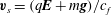 $\boldsymbol{v}_{s}=(q\boldsymbol{E}+m\boldsymbol{g})/c_{f}$
in a time of order
$\boldsymbol{v}_{s}=(q\boldsymbol{E}+m\boldsymbol{g})/c_{f}$
in a time of order
 $t_{s}$
. This time is to be compared to the residence time of the particle in its journey across the gap, of order
$t_{s}$
. This time is to be compared to the residence time of the particle in its journey across the gap, of order
 $t_{r}=L/v_{s}$
with
$t_{r}=L/v_{s}$
with
 $v_{s}=|\boldsymbol{v}_{s}|$
. In the absence of electric field,
$v_{s}=|\boldsymbol{v}_{s}|$
. In the absence of electric field,
 $v_{s}=mg/c_{f}$
and the ratio
$v_{s}=mg/c_{f}$
and the ratio
 $t_{s}/t_{r}$
is the Stokes number
$t_{s}/t_{r}$
is the Stokes number
 $St=m^{2}g/c_{f}^{2}L$
. This is typically small. For the aluminium particles of diameter
$St=m^{2}g/c_{f}^{2}L$
. This is typically small. For the aluminium particles of diameter
 $2a=10{-}30~\unicode[STIX]{x03BC}\text{m}$
used in the experiments of Shoshin & Dreizin (Reference Shoshin and Dreizin2002), it is in the range
$2a=10{-}30~\unicode[STIX]{x03BC}\text{m}$
used in the experiments of Shoshin & Dreizin (Reference Shoshin and Dreizin2002), it is in the range
 $1.12\times 10^{-3}$
–
$1.12\times 10^{-3}$
–
 $9.09\times 10^{-2}$
. The ratio
$9.09\times 10^{-2}$
. The ratio
 $t_{s}/t_{r}$
is somewhat larger than
$t_{s}/t_{r}$
is somewhat larger than
 $St$
when the electric field increases the terminal velocity, but in what follows this ratio is assumed to be also small, so that the inertia of the particle can be neglected and the momentum equation (2.3) reduces to a balance of forces.
$St$
when the electric field increases the terminal velocity, but in what follows this ratio is assumed to be also small, so that the inertia of the particle can be neglected and the momentum equation (2.3) reduces to a balance of forces.
Electrical breakdown limits the voltage that can be applied between the electrodes. Typical voltages and interelectrode distances are of the order of a few kilovolts and one centimetre, respectively, leading to electric fields of approximately one tenth of the breakdown value for air in the absence of particles. Metallic particles carrying a charge
 $q$
given by (2.1) intensify the electric field by a factor
$q$
given by (2.1) intensify the electric field by a factor
 $3+\unicode[STIX]{x1D6FC}/4\unicode[STIX]{x03C0}\approx 4.64$
. However, the small size of the region where the field is intensified may increase the breakdown value by a factor of this same order; for example, by a factor 9.7 if Rousse’s formula (Cloupeau Reference Cloupeau1994) is used for particles of
$3+\unicode[STIX]{x1D6FC}/4\unicode[STIX]{x03C0}\approx 4.64$
. However, the small size of the region where the field is intensified may increase the breakdown value by a factor of this same order; for example, by a factor 9.7 if Rousse’s formula (Cloupeau Reference Cloupeau1994) is used for particles of
 $15~\unicode[STIX]{x03BC}\text{m}$
radius. It seems thus that, unless cohesive forces are overwhelming and require the applied voltage to increase very much above the value for which the force (2.2) overcomes the weight of the particles, electrodynamic fluidization devices may operate without electrical breakdown in a certain range of voltages, except perhaps close to the electrodes or in collisions of particles with opposite charges. It was kindly pointed out by a reviewer that the possibility of electrical breakdown depends also on the presence of a resistive oxide layer around the particles, which would thus have an additional effect in the range of operation where discharges may be expected. Electrical breakdown is not taken into account in what follows.
$15~\unicode[STIX]{x03BC}\text{m}$
radius. It seems thus that, unless cohesive forces are overwhelming and require the applied voltage to increase very much above the value for which the force (2.2) overcomes the weight of the particles, electrodynamic fluidization devices may operate without electrical breakdown in a certain range of voltages, except perhaps close to the electrodes or in collisions of particles with opposite charges. It was kindly pointed out by a reviewer that the possibility of electrical breakdown depends also on the presence of a resistive oxide layer around the particles, which would thus have an additional effect in the range of operation where discharges may be expected. Electrical breakdown is not taken into account in what follows.
With many particles present in the gap, there is an upward flux of positive particles and a downward flow of negative charges. These fluxes are equal to each other in stationary conditions, as there is no net flux of particles in or out of the gap. However, owing to their weight, the upward velocity of the positive particles is smaller than the downward velocity of the negative particles, and therefore the number density of positive particles is larger than the number density of negative particles. When this effect is important, gravity leads to a net positive charge in the gap of density
 $\unicode[STIX]{x1D70C}_{e}\sim qn_{c}$
, where
$\unicode[STIX]{x1D70C}_{e}\sim qn_{c}$
, where
 $q$
is given by (2.1) and
$q$
is given by (2.1) and
 $n_{c}$
is the characteristic number density of particles. (Here the difference between the number densities of positive and negative particles is taken to be of order
$n_{c}$
is the characteristic number density of particles. (Here the difference between the number densities of positive and negative particles is taken to be of order
 $n_{c}$
, but see § 3 below for more accurate results.) The electric field induced by this space charge is
$n_{c}$
, but see § 3 below for more accurate results.) The electric field induced by this space charge is
 $E_{sc}\sim qn_{c}L/\unicode[STIX]{x1D716}_{0}$
, from the Poisson equation
$E_{sc}\sim qn_{c}L/\unicode[STIX]{x1D716}_{0}$
, from the Poisson equation
 $\unicode[STIX]{x1D6FB}^{2}\unicode[STIX]{x1D711}=-\unicode[STIX]{x1D70C}_{e}/\unicode[STIX]{x1D716}_{0}$
, where
$\unicode[STIX]{x1D6FB}^{2}\unicode[STIX]{x1D711}=-\unicode[STIX]{x1D70C}_{e}/\unicode[STIX]{x1D716}_{0}$
, where
 $\unicode[STIX]{x1D711}$
is the electric potential (
$\unicode[STIX]{x1D711}$
is the electric potential (
 $\boldsymbol{E}=-\unicode[STIX]{x1D735}\unicode[STIX]{x1D711}$
). Using (2.1), the ratio of this field to the field due to the applied voltage is
$\boldsymbol{E}=-\unicode[STIX]{x1D735}\unicode[STIX]{x1D711}$
). Using (2.1), the ratio of this field to the field due to the applied voltage is
 $E_{sc}/E\sim n_{c}a^{2}L$
. Thus the presence of charged particles significantly affects the electric field when
$E_{sc}/E\sim n_{c}a^{2}L$
. Thus the presence of charged particles significantly affects the electric field when
 $n_{c}\sim 1/(a^{2}L)$
.
$n_{c}\sim 1/(a^{2}L)$
.
Particles with different charges move in the gap with different velocities and eventually collide, redistributing their charges and leading to new populations with charges different from the charges acquired by the particles at the lower and upper electrodes. Leaving out the electrostatic force between colliding particles (see appendix A), the cross-section for mechanical collisions of any two particles is
 $\unicode[STIX]{x1D70E}=4\unicode[STIX]{x03C0}a^{2}$
. Consider a particle from a population
$\unicode[STIX]{x1D70E}=4\unicode[STIX]{x03C0}a^{2}$
. Consider a particle from a population
 $i$
with charge
$i$
with charge
 $q_{i}$
and number density
$q_{i}$
and number density
 $n_{i}$
, moving with velocity
$n_{i}$
, moving with velocity
 $\boldsymbol{v}_{i}$
across a region with a number density
$\boldsymbol{v}_{i}$
across a region with a number density
 $n_{j}$
of particles with charge
$n_{j}$
of particles with charge
 $q_{j}$
and velocity
$q_{j}$
and velocity
 $\boldsymbol{v}_{j}$
. The mean free path of the particle considered between collisions with particles of population
$\boldsymbol{v}_{j}$
. The mean free path of the particle considered between collisions with particles of population
 $j$
is
$j$
is
 $\unicode[STIX]{x1D706}_{ij}=1/(\unicode[STIX]{x1D70E}n_{j})$
. The mean number of collisions of this particle per unit time is
$\unicode[STIX]{x1D706}_{ij}=1/(\unicode[STIX]{x1D70E}n_{j})$
. The mean number of collisions of this particle per unit time is
 $|\boldsymbol{v}_{i}-\boldsymbol{v}_{j}|/\unicode[STIX]{x1D706}_{ij}$
, and the mean number of collisions of the whole population
$|\boldsymbol{v}_{i}-\boldsymbol{v}_{j}|/\unicode[STIX]{x1D706}_{ij}$
, and the mean number of collisions of the whole population
 $i$
to which the particle belongs with particles of population
$i$
to which the particle belongs with particles of population
 $j$
per unit volume and time is
$j$
per unit volume and time is
 $w_{ij}=4\unicode[STIX]{x03C0}a^{2}|\boldsymbol{v}_{i}-\boldsymbol{v}_{j}|n_{i}n_{j}$
. For particles of high electrical conductivity, each of these collisions removes one particle of population
$w_{ij}=4\unicode[STIX]{x03C0}a^{2}|\boldsymbol{v}_{i}-\boldsymbol{v}_{j}|n_{i}n_{j}$
. For particles of high electrical conductivity, each of these collisions removes one particle of population
 $i$
and one particle of population
$i$
and one particle of population
 $j$
, and generates two particles with charges
$j$
, and generates two particles with charges
 $(q_{i}+q_{j})/2\pm q_{E}$
, where
$(q_{i}+q_{j})/2\pm q_{E}$
, where
 $q_{E}$
is the excess or defect of charge induced in the colliding particles by the electric field at the point where the collision takes place; see appendix A.
$q_{E}$
is the excess or defect of charge induced in the colliding particles by the electric field at the point where the collision takes place; see appendix A.
Collisions significantly change the number density of each population during their journey across the gap when the mean free path for collisions with particles of any other population is of order
 $L$
. In terms of the characteristic number density of particles in the gap, this condition reads
$L$
. In terms of the characteristic number density of particles in the gap, this condition reads
 $1/(\unicode[STIX]{x1D70E}n_{c})\sim L$
, or
$1/(\unicode[STIX]{x1D70E}n_{c})\sim L$
, or
 $n_{c}\sim 1/(a^{2}L)$
. Thus, in the coarse approximation used here, the condition for collisions to matter coincides with the condition above for the electric field induced by the charge of the particles to be of the order of the field due to the applied voltage. When this condition is satisfied, the mean distance between particles is
$n_{c}\sim 1/(a^{2}L)$
. Thus, in the coarse approximation used here, the condition for collisions to matter coincides with the condition above for the electric field induced by the charge of the particles to be of the order of the field due to the applied voltage. When this condition is satisfied, the mean distance between particles is
 $1/n_{c}^{1/3}\sim a(L/a)^{1/3}\gg a$
. The suspension is still dilute, which justifies neglecting correlations between particles and three-body collisions.
$1/n_{c}^{1/3}\sim a(L/a)^{1/3}\gg a$
. The suspension is still dilute, which justifies neglecting correlations between particles and three-body collisions.
At small Stokes numbers, in the absence of particle inertia, the electric and gravity forces acting on each particle are balanced by its hydrodynamic drag. These forces are thus transmitted to the gas and set it in motion. Assuming that the gravity force is representative of the total force acting on a particle, the force of the particles on the gas is of order
 $n_{c}mg$
per unit volume, where
$n_{c}mg$
per unit volume, where
 $n_{c}$
denotes again the characteristic number density of particles in the gap. An order-of-magnitude balance of this force and the inertia of the gas reads
$n_{c}$
denotes again the characteristic number density of particles in the gap. An order-of-magnitude balance of this force and the inertia of the gas reads
 $\unicode[STIX]{x1D70C}_{g}v_{g}^{2}/L\sim n_{c}mg$
, where
$\unicode[STIX]{x1D70C}_{g}v_{g}^{2}/L\sim n_{c}mg$
, where
 $\unicode[STIX]{x1D70C}_{g}$
is the density of the gas and
$\unicode[STIX]{x1D70C}_{g}$
is the density of the gas and
 $v_{g}$
is its characteristic velocity. Using the settling velocity
$v_{g}$
is its characteristic velocity. Using the settling velocity
 $v_{s}=mg/c_{f}$
, this balance gives
$v_{s}=mg/c_{f}$
, this balance gives
 $v_{g}/v_{s}\sim 6\unicode[STIX]{x03C0}(n_{c}a^{2}L)^{1/2}(\unicode[STIX]{x1D707}_{g}^{2}/\unicode[STIX]{x1D70C}_{g}mg)^{1/2}$
, which is large when
$v_{g}/v_{s}\sim 6\unicode[STIX]{x03C0}(n_{c}a^{2}L)^{1/2}(\unicode[STIX]{x1D707}_{g}^{2}/\unicode[STIX]{x1D70C}_{g}mg)^{1/2}$
, which is large when
 $n_{c}a^{2}L=O(1)$
, of the order of 16–30 in the experiments of Shoshin & Dreizin (Reference Shoshin and Dreizin2002). This result overestimates the velocity of the gas in cases when the force of the particles can be balanced by a hydrostatic pressure or when there is much cancellation of the forces of positive and negative particles (see § 3 below), but it shows the potential of the induced gas flow to affect the dynamics of the aerosol. The Reynolds number of the gas flow,
$n_{c}a^{2}L=O(1)$
, of the order of 16–30 in the experiments of Shoshin & Dreizin (Reference Shoshin and Dreizin2002). This result overestimates the velocity of the gas in cases when the force of the particles can be balanced by a hydrostatic pressure or when there is much cancellation of the forces of positive and negative particles (see § 3 below), but it shows the potential of the induced gas flow to affect the dynamics of the aerosol. The Reynolds number of the gas flow,
 $\unicode[STIX]{x1D70C}_{g}v_{g}L/\unicode[STIX]{x1D707}_{g}$
, is in the range 380–470 in the conditions of the experiments of Shoshin & Dreizin when
$\unicode[STIX]{x1D70C}_{g}v_{g}L/\unicode[STIX]{x1D707}_{g}$
, is in the range 380–470 in the conditions of the experiments of Shoshin & Dreizin when
 $n_{c}a^{2}L=O(1)$
.
$n_{c}a^{2}L=O(1)$
.
2.2 Governing equations
In the absence of particle inertia, a monodisperse aerosol may be characterized by its one-particle distribution function
 $f(\boldsymbol{x},q,t)$
, such that the mean number of particles in the volume between
$f(\boldsymbol{x},q,t)$
, such that the mean number of particles in the volume between
 $\boldsymbol{x}$
and
$\boldsymbol{x}$
and
 $\boldsymbol{x}+\text{d}\boldsymbol{x}$
with charge between
$\boldsymbol{x}+\text{d}\boldsymbol{x}$
with charge between
 $q$
and
$q$
and
 $q+\text{d}q$
is
$q+\text{d}q$
is
 $f(\boldsymbol{x},q,t)\,\text{d}\boldsymbol{x}\,\text{d}q$
at time
$f(\boldsymbol{x},q,t)\,\text{d}\boldsymbol{x}\,\text{d}q$
at time
 $t$
. Leaving out collisions and neglecting correlations between particles, this function would satisfy a Vlasov equation (Landau & Lifshitz Reference Landau and Lifshitz1981; Clemmow & Dougherty Reference Clemmow and Dougherty1990) involving self-consistent mesoscale electric and gas velocity fields,
$t$
. Leaving out collisions and neglecting correlations between particles, this function would satisfy a Vlasov equation (Landau & Lifshitz Reference Landau and Lifshitz1981; Clemmow & Dougherty Reference Clemmow and Dougherty1990) involving self-consistent mesoscale electric and gas velocity fields,
 $\boldsymbol{E}$
and
$\boldsymbol{E}$
and
 $\boldsymbol{v}_{g}$
. If the collisions responsible for charge redistribution are instantaneous events, they can be added to this equation to give
$\boldsymbol{v}_{g}$
. If the collisions responsible for charge redistribution are instantaneous events, they can be added to this equation to give
 $$\begin{eqnarray}\frac{\unicode[STIX]{x2202}f}{\unicode[STIX]{x2202}t}+\unicode[STIX]{x1D735}\boldsymbol{\cdot }(\boldsymbol{v}f)={\mathcal{C}}\quad \text{with }\boldsymbol{v}=\boldsymbol{v}_{g}+\frac{q\boldsymbol{E}+m\boldsymbol{g}}{c_{f}},\end{eqnarray}$$
where the collision term
 ${\mathcal{C}}$
can be decomposed into the negative contribution of collisions that remove particles with charge
${\mathcal{C}}$
can be decomposed into the negative contribution of collisions that remove particles with charge
 $q$
and the positive contribution of collisions that generate particles with charge
$q$
and the positive contribution of collisions that generate particles with charge
 $q$
;
$q$
;
 ${\mathcal{C}}={\mathcal{C}}^{-}+{\mathcal{C}}^{+}$
. The first of these contributions is (with
${\mathcal{C}}={\mathcal{C}}^{-}+{\mathcal{C}}^{+}$
. The first of these contributions is (with
 $E=|\boldsymbol{E}|$
)
$E=|\boldsymbol{E}|$
)
 $$\begin{eqnarray}\displaystyle {\mathcal{C}}^{-}(\boldsymbol{x},q) & = & \displaystyle -4\unicode[STIX]{x03C0}a^{2}f(\boldsymbol{x},q)\int _{-\infty }^{\infty }|\boldsymbol{v}-\boldsymbol{v}^{\prime }|f(\boldsymbol{x},q^{\prime })\,\text{d}q^{\prime }\nonumber\\ \displaystyle & = & \displaystyle -\frac{4\unicode[STIX]{x03C0}a^{2}E}{c_{f}}f(\boldsymbol{x},q)\int _{-\infty }^{\infty }|q-q^{\prime }|f(\boldsymbol{x},q^{\prime })\,\text{d}q^{\prime },\end{eqnarray}$$
where
 $4\unicode[STIX]{x03C0}a^{2}|\boldsymbol{v}-\boldsymbol{v}^{\prime }|$
is the volume swept per unit time by a particle with charge
$4\unicode[STIX]{x03C0}a^{2}|\boldsymbol{v}-\boldsymbol{v}^{\prime }|$
is the volume swept per unit time by a particle with charge
 $q$
in a reference frame in which particles with charge
$q$
in a reference frame in which particles with charge
 $q^{\prime }$
are at rest. The dependence of
$q^{\prime }$
are at rest. The dependence of
 $f$
,
$f$
,
 ${\mathcal{C}}$
and other variables on time is not indicated explicitly hereafter. The integral accounts for collisions in which the particle with charge
${\mathcal{C}}$
and other variables on time is not indicated explicitly hereafter. The integral accounts for collisions in which the particle with charge
 $q$
overtakes that with charge
$q$
overtakes that with charge
 $q^{\prime }$
(when
$q^{\prime }$
(when
 $q>q^{\prime }$
) and those in which the opposite occurs (when
$q>q^{\prime }$
) and those in which the opposite occurs (when
 $q^{\prime }>q$
). The contribution of collisions that generate particles with charge
$q^{\prime }>q$
). The contribution of collisions that generate particles with charge
 $q$
is
$q$
is
 $$\begin{eqnarray}\displaystyle {\mathcal{C}}^{+} & = & \displaystyle \int _{0}^{2a}\int _{-\infty }^{\infty }f(\boldsymbol{x},q+q^{\prime }+2q_{E})f(\boldsymbol{x},q-q^{\prime })\frac{2|q^{\prime }+q_{E}|E}{c_{f}}2\unicode[STIX]{x03C0}e\,\text{d}e\,\text{d}q^{\prime }\nonumber\\ \displaystyle & & \displaystyle +\,\int _{0}^{2a}\int _{-\infty }^{\infty }f(\boldsymbol{x},q+q^{\prime })f(\boldsymbol{x},q-q^{\prime }-2q_{E})\frac{2|q^{\prime }+q_{E}|E}{c_{f}}2\unicode[STIX]{x03C0}e\,\text{d}e\,\text{d}q^{\prime }.\end{eqnarray}$$
Here the first integral accounts for collisions of particles with charges
 $q+q^{\prime }+2q_{E}$
and
$q+q^{\prime }+2q_{E}$
and
 $q-q^{\prime }$
, with
$q-q^{\prime }$
, with
 $q_{E}$
given by (A 2). The relative velocity between these particles is
$q_{E}$
given by (A 2). The relative velocity between these particles is
 $2|q^{\prime }+q_{E}|E/c_{f}$
. As explained in appendix A, each of these collisions generates a particle with charge
$2|q^{\prime }+q_{E}|E/c_{f}$
. As explained in appendix A, each of these collisions generates a particle with charge
 $q+2q_{E}$
and another with charge
$q+2q_{E}$
and another with charge
 $q$
. The integral over the impact parameter
$q$
. The integral over the impact parameter
 $e$
must be included explicitly because
$e$
must be included explicitly because
 $q_{E}$
depends on this parameter. Similarly, the second integral accounts for collisions of particles with charges
$q_{E}$
depends on this parameter. Similarly, the second integral accounts for collisions of particles with charges
 $q+q^{\prime }$
and
$q+q^{\prime }$
and
 $q-q^{\prime }-2q_{E}$
, whose outcome is a particle with charge
$q-q^{\prime }-2q_{E}$
, whose outcome is a particle with charge
 $q$
and another with charge
$q$
and another with charge
 $q-2q_{E}$
.
$q-2q_{E}$
.
Equation (2.6) is difficult to use owing to the dependence of
 $q_{E}$
on the impact parameter
$q_{E}$
on the impact parameter
 $e$
. Here this equation is simplified by assuming that
$e$
. Here this equation is simplified by assuming that
 $q_{E}$
is small compared to the typical charges of the colliding particles. Then the integrands in (2.6) can be Taylor expanded and the result, at leading order, can be written in terms of the mean value of
$q_{E}$
is small compared to the typical charges of the colliding particles. Then the integrands in (2.6) can be Taylor expanded and the result, at leading order, can be written in terms of the mean value of
 $q_{E}$
given by (A 3) as
$q_{E}$
given by (A 3) as
 $$\begin{eqnarray}\displaystyle {\mathcal{C}}^{+} & {\approx} & \displaystyle \frac{8\unicode[STIX]{x03C0}a^{2}E}{c_{f}}\int _{-\infty }^{\infty }[f(\boldsymbol{x},q+q^{\prime }+2\bar{q}_{E})f(\boldsymbol{x},q-q^{\prime })\nonumber\\ \displaystyle & & \displaystyle +\;f(\boldsymbol{x},q+q^{\prime })f(\boldsymbol{x},q-q^{\prime }-2\bar{q}_{E})\!]|q^{\prime }+\bar{q}_{E}|\,\text{d}q^{\prime }.\end{eqnarray}$$
Since the charge of the particles is of order
 $\unicode[STIX]{x1D6FC}\unicode[STIX]{x1D716}_{0}a^{2}E_{c}$
where
$\unicode[STIX]{x1D6FC}\unicode[STIX]{x1D716}_{0}a^{2}E_{c}$
where
 $E_{c}$
is the characteristic value of the electric field (cf. (2.1)), while
$E_{c}$
is the characteristic value of the electric field (cf. (2.1)), while
 $\bar{q}_{E}=O(\unicode[STIX]{x1D6FE}\unicode[STIX]{x1D716}_{0}a^{2}E_{c})$
(cf. (A 3)), the simplification (2.7) amounts to assuming that
$\bar{q}_{E}=O(\unicode[STIX]{x1D6FE}\unicode[STIX]{x1D716}_{0}a^{2}E_{c})$
(cf. (A 3)), the simplification (2.7) amounts to assuming that
 $\unicode[STIX]{x1D6FC}$
is large compared to
$\unicode[STIX]{x1D6FC}$
is large compared to
 $\unicode[STIX]{x1D6FE}$
. This involves a noticeable error, but (2.7) is expected to retain the main features of the much more complex collision rate (2.6).
$\unicode[STIX]{x1D6FE}$
. This involves a noticeable error, but (2.7) is expected to retain the main features of the much more complex collision rate (2.6).
Conservation of the number of particles and the charge in collisions requires
 $\int {\mathcal{C}}(\boldsymbol{x},q)\,\text{d}q=0$
and
$\int {\mathcal{C}}(\boldsymbol{x},q)\,\text{d}q=0$
and
 $\int q{\mathcal{C}}(\boldsymbol{x},q)\,\text{d}q=0$
. Using these conditions, the first moments of the kinetic equation (2.4) give the mass and charge conservation equations
$\int q{\mathcal{C}}(\boldsymbol{x},q)\,\text{d}q=0$
. Using these conditions, the first moments of the kinetic equation (2.4) give the mass and charge conservation equations
 $$\begin{eqnarray}\left.\begin{array}{@{}c@{}}\displaystyle \frac{\unicode[STIX]{x2202}n}{\unicode[STIX]{x2202}t}+\unicode[STIX]{x1D735}\boldsymbol{\cdot }\boldsymbol{p}=0\quad \text{and}\quad \frac{\unicode[STIX]{x2202}\unicode[STIX]{x1D70C}_{e}}{\unicode[STIX]{x2202}t}+\unicode[STIX]{x1D735}\boldsymbol{\cdot }\boldsymbol{j}=0\quad \text{with }\\ \displaystyle n=\int f\,\text{d}q,\quad \unicode[STIX]{x1D70C}_{e}=\int qf\,\text{d}q,\quad \boldsymbol{p}=\int \boldsymbol{v}f\,\text{d}q,\quad \boldsymbol{j}=\int q\boldsymbol{v}f\,\text{d}q.\end{array}\right\}\end{eqnarray}$$
The self-consistent electric field in the kinetic equation (2.4) is
 $\boldsymbol{E}=-\unicode[STIX]{x1D735}\unicode[STIX]{x1D711}$
, where the mesoscale electric potential
$\boldsymbol{E}=-\unicode[STIX]{x1D735}\unicode[STIX]{x1D711}$
, where the mesoscale electric potential
 $\unicode[STIX]{x1D711}$
satisfies the Poisson equation (see e.g. Clemmow & Dougherty Reference Clemmow and Dougherty1990)
$\unicode[STIX]{x1D711}$
satisfies the Poisson equation (see e.g. Clemmow & Dougherty Reference Clemmow and Dougherty1990)
 $$\begin{eqnarray}\unicode[STIX]{x1D6FB}^{2}\unicode[STIX]{x1D711}=-\frac{\unicode[STIX]{x1D70C}_{e}}{\unicode[STIX]{x1D716}_{0}},\end{eqnarray}$$
Equations for the mesoscale flow of the gas may be derived from the principles of conservation of mass and momentum applied to the gas in an elementary control volume of size large compared to the mean distance between particles but small compared to
 $L$
(Williams Reference Williams1985). This volume contains many particles exchanging momentum with the gas, whose effect appears as a distributed force in the gas momentum equation. The mesoscale gas velocity and pressure,
$L$
(Williams Reference Williams1985). This volume contains many particles exchanging momentum with the gas, whose effect appears as a distributed force in the gas momentum equation. The mesoscale gas velocity and pressure,
 $\boldsymbol{v}_{g}$
and
$\boldsymbol{v}_{g}$
and
 $p_{g}$
, thus satisfy the conservation equations (Williams Reference Williams1985)
$p_{g}$
, thus satisfy the conservation equations (Williams Reference Williams1985)
 $$\begin{eqnarray}\left.\begin{array}{@{}c@{}}\displaystyle \unicode[STIX]{x1D735}\boldsymbol{\cdot }\boldsymbol{v}_{g}=0,\quad \unicode[STIX]{x1D70C}_{g}\frac{\text{D}\boldsymbol{v}_{g}}{\text{D}t}=-\unicode[STIX]{x1D735}p_{g}+\unicode[STIX]{x1D707}_{g}\unicode[STIX]{x1D6FB}^{2}\boldsymbol{v}_{g}+\boldsymbol{F}\\ \displaystyle \text{with }\boldsymbol{F}(\boldsymbol{x})=\int c_{f}(\boldsymbol{v}-\boldsymbol{v}_{g})f(\boldsymbol{x},q)\,\text{d}q,\end{array}\right\}\end{eqnarray}$$
with
 $\text{D}\boldsymbol{v}_{g}/\text{D}t=\unicode[STIX]{x2202}\boldsymbol{v}_{g}/\unicode[STIX]{x2202}t+\boldsymbol{v}_{g}\boldsymbol{\cdot }\unicode[STIX]{x1D735}\boldsymbol{v}_{g}$
.
$\text{D}\boldsymbol{v}_{g}/\text{D}t=\unicode[STIX]{x2202}\boldsymbol{v}_{g}/\unicode[STIX]{x2202}t+\boldsymbol{v}_{g}\boldsymbol{\cdot }\unicode[STIX]{x1D735}\boldsymbol{v}_{g}$
.
In the operation of an electrodynamic fluidization device an excess of particles is often deposited at the lower electrode. The electric force continuously detaches these particles until the space charge due to the particles in suspension reduces the electric field at the electrode to the threshold value below which the electric force could no longer overcome the weight of the particles that bounce off the electrode. In this stationary state, the particles that fall onto the electrode are replaced by particles that detach from it with the equilibrium charge
 $q_{+}=\unicode[STIX]{x1D6FC}\unicode[STIX]{x1D716}_{0}a^{2}E$
, where
$q_{+}=\unicode[STIX]{x1D6FC}\unicode[STIX]{x1D716}_{0}a^{2}E$
, where
 $E$
is the threshold field satisfying
$E$
is the threshold field satisfying
 $q_{+}E=mg$
. Here, rather than directly trying to compute this state, it will be assumed that there are no particles deposited at the lower electrode and that the number of suspended particles in the interelectrode space is a given constant,
$q_{+}E=mg$
. Here, rather than directly trying to compute this state, it will be assumed that there are no particles deposited at the lower electrode and that the number of suspended particles in the interelectrode space is a given constant,
 $$\begin{eqnarray}\int f(\boldsymbol{x},q)\,\text{d}\boldsymbol{x}\,\text{d}q=NA,\end{eqnarray}$$
where
 $A$
is the area of the electrodes, the integral extends to the whole interelectrode volume, and
$A$
is the area of the electrodes, the integral extends to the whole interelectrode volume, and
 $N$
is the number of suspended particles per unit electrode area. A stationary solution satisfying this condition exists only when the applied voltage is higher than a certain value for which the electric field at the lower electrode equals the threshold value mentioned above. This minimum voltage is found in the following section as a function of
$N$
is the number of suspended particles per unit electrode area. A stationary solution satisfying this condition exists only when the applied voltage is higher than a certain value for which the electric field at the lower electrode equals the threshold value mentioned above. This minimum voltage is found in the following section as a function of
 $N$
and the parameters of the problem. Upon inverting this function, the value of
$N$
and the parameters of the problem. Upon inverting this function, the value of
 $N$
in the normal stationary operation of the device can be found as a function of the applied voltage.
$N$
in the normal stationary operation of the device can be found as a function of the applied voltage.
Cartesian coordinates will be used, with the distance
 $x$
measured upwards from the lower electrode, so that
$x$
measured upwards from the lower electrode, so that
 $\boldsymbol{g}=-g\hat{\boldsymbol{\imath }}$
with
$\boldsymbol{g}=-g\hat{\boldsymbol{\imath }}$
with
 $\hat{\boldsymbol{\imath }}$
a unit vector pointing upwards.
$\hat{\boldsymbol{\imath }}$
a unit vector pointing upwards.
Equations (2.4), (2.5), (2.7), (2.9) and (2.10) must be solved with the boundary conditions
 $$\begin{eqnarray}\left.\begin{array}{@{}c@{}}\displaystyle f=f_{+}\unicode[STIX]{x1D6FF}(q-q_{+})\quad \text{for }v_{x}>0\text{ with }q_{+}=\unicode[STIX]{x1D6FC}\unicode[STIX]{x1D716}_{0}a^{2}E,\quad f_{+}\frac{q_{+}E-mg}{c_{f}}=\unicode[STIX]{x1D719}_{+}\\ \displaystyle \unicode[STIX]{x1D711}=0,\quad \boldsymbol{v}_{g}=0\end{array}\right\}\end{eqnarray}$$
at the lower electrode,
 $x=0$
, where the first equation expresses the condition that the particles impinging on this electrode, whose flux is
$x=0$
, where the first equation expresses the condition that the particles impinging on this electrode, whose flux is
 $\unicode[STIX]{x1D719}_{+}=-\int _{v_{x}<0}v_{x}f\,\text{d}q$
, immediately acquire a charge
$\unicode[STIX]{x1D719}_{+}=-\int _{v_{x}<0}v_{x}f\,\text{d}q$
, immediately acquire a charge
 $q_{+}$
and are reinjected into the gap, and, similarly,
$q_{+}$
and are reinjected into the gap, and, similarly,
 $$\begin{eqnarray}\left.\begin{array}{@{}c@{}}\displaystyle f=f_{-}\unicode[STIX]{x1D6FF}(q-q_{-})\quad \text{for }v_{x}<0\text{ with }q_{-}=-\unicode[STIX]{x1D6FC}\unicode[STIX]{x1D716}_{0}a^{2}E,\quad f_{-}\frac{q_{-}E-mg}{c_{f}}=-\unicode[STIX]{x1D719}_{-}\\ \unicode[STIX]{x1D711}=-V,\quad \boldsymbol{v}_{g}=0\end{array}\right\}\end{eqnarray}$$
at the upper electrode,
 $x=L$
, where
$x=L$
, where
 $\unicode[STIX]{x1D719}_{-}=\int _{v_{x}>0}v_{x}f\,\text{d}q$
is the flux of particles impinging on this electrode. In addition, conditions of periodicity are used in the directions parallel to the electrodes to approximately simulate a region of the interelectrode gap.
$\unicode[STIX]{x1D719}_{-}=\int _{v_{x}>0}v_{x}f\,\text{d}q$
is the flux of particles impinging on this electrode. In addition, conditions of periodicity are used in the directions parallel to the electrodes to approximately simulate a region of the interelectrode gap.
In what follows, distances are scaled with the interelectrode distance
 $L$
, velocities with the settling velocity in the absence of electric field,
$L$
, velocities with the settling velocity in the absence of electric field,
 $mg/c_{f}$
, and time with
$mg/c_{f}$
, and time with
 $c_{f}L/mg$
. The electric field and the electric charge are scaled with
$c_{f}L/mg$
. The electric field and the electric charge are scaled with
 $E_{m}$
and
$E_{m}$
and
 $q_{m}=\unicode[STIX]{x1D6FC}\unicode[STIX]{x1D716}_{0}a^{2}E_{m}$
, where
$q_{m}=\unicode[STIX]{x1D6FC}\unicode[STIX]{x1D716}_{0}a^{2}E_{m}$
, where
 $E_{m}=\sqrt{mg/\unicode[STIX]{x1D6FC}\unicode[STIX]{x1D716}_{0}a^{2}}$
is the solution of
$E_{m}=\sqrt{mg/\unicode[STIX]{x1D6FC}\unicode[STIX]{x1D716}_{0}a^{2}}$
is the solution of
 $q_{+}E_{m}=mg$
. The electric potential
$q_{+}E_{m}=mg$
. The electric potential
 $\unicode[STIX]{x1D711}$
is scaled with
$\unicode[STIX]{x1D711}$
is scaled with
 $E_{m}L$
and the distribution function with
$E_{m}L$
and the distribution function with
 $1/(\unicode[STIX]{x1D6FC}La^{2}q_{m})$
. Accordingly, the number and charge densities and the momentum (per unit mass) and current density that appear in (2.8) are scaled with [
$1/(\unicode[STIX]{x1D6FC}La^{2}q_{m})$
. Accordingly, the number and charge densities and the momentum (per unit mass) and current density that appear in (2.8) are scaled with [
 $1/(\unicode[STIX]{x1D6FC}La^{2})$
,
$1/(\unicode[STIX]{x1D6FC}La^{2})$
,
 $q_{m}/(\unicode[STIX]{x1D6FC}La^{2})$
,
$q_{m}/(\unicode[STIX]{x1D6FC}La^{2})$
,
 $mg/(\unicode[STIX]{x1D6FC}La^{2}c_{f})$
,
$mg/(\unicode[STIX]{x1D6FC}La^{2}c_{f})$
,
 $q_{m}mg/(\unicode[STIX]{x1D6FC}La^{2})$
], and the voltage
$q_{m}mg/(\unicode[STIX]{x1D6FC}La^{2})$
], and the voltage
 $V$
and
$V$
and
 $N$
with
$N$
with
 $E_{m}L$
and
$E_{m}L$
and
 $1/(\unicode[STIX]{x1D6FC}a^{2})$
. Here
$1/(\unicode[STIX]{x1D6FC}a^{2})$
. Here
 $E_{m}$
is the electric field that would be required at the lower electrode for the electric force on a bouncing particle to exactly balance its weight. As explained above, this is the minimum value that the electric field may have in stationary conditions; smaller values would not suffice to pull the bouncing particles upwards.
$E_{m}$
is the electric field that would be required at the lower electrode for the electric force on a bouncing particle to exactly balance its weight. As explained above, this is the minimum value that the electric field may have in stationary conditions; smaller values would not suffice to pull the bouncing particles upwards.
Using the same symbols to denote the dimensionless variables and their dimensional counterparts, which will no longer appear, equations (2.4), (2.5), (2.7), (2.9)–(2.11) become
 $$\begin{eqnarray}\left.\begin{array}{@{}c@{}}\begin{array}{@{}c@{}}\displaystyle \frac{\unicode[STIX]{x2202}f}{\unicode[STIX]{x2202}t}+\unicode[STIX]{x1D735}\boldsymbol{\cdot }(\boldsymbol{v}f)=\frac{{\mathcal{C}}}{\unicode[STIX]{x1D6FC}}\quad \text{with }\boldsymbol{v}=\boldsymbol{v}_{g}+q\boldsymbol{E}-\hat{\boldsymbol{\imath }}\quad \text{and}\end{array}\\ \begin{array}{@{}rcl@{}}\displaystyle {\mathcal{C}}\; & =\; & \displaystyle -4\unicode[STIX]{x03C0}Ef(\boldsymbol{x},q)\int |q-q^{\prime }|f(\boldsymbol{x},q^{\prime })\,\text{d}q^{\prime }\\ \displaystyle \; & \; & +\,\displaystyle 8\unicode[STIX]{x03C0}E\int [f(\boldsymbol{x},q+q^{\prime }+2\bar{q}_{E})f(\boldsymbol{x},q-q^{\prime })\\ \displaystyle \; & \; & +\;\displaystyle f(\boldsymbol{x},q+q^{\prime })f(\boldsymbol{x},q-q^{\prime }-2\bar{q}_{E})\!]|q^{\prime }+\bar{q}_{E}|\,\text{d}q^{\prime },\end{array}\end{array}\right\}\end{eqnarray}$$
 $$\begin{eqnarray}\unicode[STIX]{x1D6FB}^{2}\unicode[STIX]{x1D711}=-\unicode[STIX]{x1D70C}_{e}\quad \text{with }\unicode[STIX]{x1D70C}_{e}=\int qf(\boldsymbol{x},q)\,\text{d}q\quad \text{and}\quad \boldsymbol{E}=-\unicode[STIX]{x1D735}\unicode[STIX]{x1D711},\end{eqnarray}$$
 $$\begin{eqnarray}\left.\begin{array}{@{}c@{}}\displaystyle \unicode[STIX]{x1D735}\boldsymbol{\cdot }\boldsymbol{v}_{g}=0,\quad R\frac{\text{D}\boldsymbol{v}_{g}}{\text{D}t}=-\unicode[STIX]{x1D735}p_{g}+\unicode[STIX]{x1D6FB}^{2}\boldsymbol{v}_{g}+\boldsymbol{F}\\ \displaystyle \text{with}\quad \boldsymbol{F}(\boldsymbol{x})=\frac{1}{\unicode[STIX]{x1D6FC}\widetilde{a}}\int (q\boldsymbol{E}-\hat{\boldsymbol{\imath }})f(\boldsymbol{x},q)\,\text{d}q,\end{array}\right\}\end{eqnarray}$$
 $$\begin{eqnarray}\frac{1}{\widetilde{A}}\int f\,\text{d}\boldsymbol{x}\,\text{d}q=N,\end{eqnarray}$$
and the boundary conditions (2.12) and (2.13) become
 $$\begin{eqnarray}\left.\begin{array}{@{}c@{}}\displaystyle f=f_{+}\unicode[STIX]{x1D6FF}(q-q_{+})\quad \text{for }qE-1>0\text{ with }q_{+}=E,\quad f_{+}(q_{+}E-1)=-\int _{v_{x}<0}v_{x}f\,\text{d}q\\ \displaystyle \unicode[STIX]{x1D711}=0,\quad \boldsymbol{v}_{g}=0\end{array}\right\}\end{eqnarray}$$
at
 $x=0$
and
$x=0$
and
 $$\begin{eqnarray}\left.\begin{array}{@{}c@{}}\displaystyle f=f_{-}\unicode[STIX]{x1D6FF}(q-q_{-})\quad \text{for }qE-1<0\text{ with }q_{-}=-E,\quad f_{-}(q_{-}E-1)=-\int _{v_{x}>0}v_{x}f\,\text{d}q\\ \displaystyle \unicode[STIX]{x1D711}=-V,\quad \boldsymbol{v}_{g}=0\end{array}\right\}\end{eqnarray}$$
at
 $x=1$
. The solution depends on the five dimensionless parameters
$x=1$
. The solution depends on the five dimensionless parameters
 $$\begin{eqnarray}N,V,R=\frac{\unicode[STIX]{x1D70C}_{g}mgL}{6\unicode[STIX]{x03C0}\unicode[STIX]{x1D707}_{g}^{2}a},\quad \widetilde{a}=\frac{a/L}{6\unicode[STIX]{x03C0}}\quad \text{and}\quad \widetilde{A}=\frac{A}{L^{2}}\end{eqnarray}$$
and the constant
 $\unicode[STIX]{x1D6FC}=2\unicode[STIX]{x03C0}^{3}/3$
. Here
$\unicode[STIX]{x1D6FC}=2\unicode[STIX]{x03C0}^{3}/3$
. Here
 $N$
is the number of suspended particles per unit electrode area scaled with
$N$
is the number of suspended particles per unit electrode area scaled with
 $1/(\unicode[STIX]{x1D6FC}a^{2})$
,
$1/(\unicode[STIX]{x1D6FC}a^{2})$
,
 $V$
is the voltage applied between the electrodes scaled with
$V$
is the voltage applied between the electrodes scaled with
 $\sqrt{mg/\unicode[STIX]{x1D6FC}\unicode[STIX]{x1D716}_{0}a^{2}}L$
,
$\sqrt{mg/\unicode[STIX]{x1D6FC}\unicode[STIX]{x1D716}_{0}a^{2}}L$
,
 $R$
is a Reynolds number of the mesoscale gas flow,
$R$
is a Reynolds number of the mesoscale gas flow,
 $\widetilde{a}$
is the radius of the particles scaled with
$\widetilde{a}$
is the radius of the particles scaled with
 $6\unicode[STIX]{x03C0}L$
, where the factor
$6\unicode[STIX]{x03C0}L$
, where the factor
 $6\unicode[STIX]{x03C0}$
is introduced for convenience, and
$6\unicode[STIX]{x03C0}$
is introduced for convenience, and
 $\widetilde{A}$
is the electrode area scaled with the square of the interelectrode distance.
$\widetilde{A}$
is the electrode area scaled with the square of the interelectrode distance.
3 Stationary solutions
Stationary solutions for unbounded electrodes depend only on the vertical distance
 $x$
and have vertical velocities and electric field, which will be denoted
$x$
and have vertical velocities and electric field, which will be denoted
 $v_{i}(x)$
and
$v_{i}(x)$
and
 $E(x)$
. The electric current carried by the particles across the unit area of any horizontal section of the gap is a constant,
$E(x)$
. The electric current carried by the particles across the unit area of any horizontal section of the gap is a constant,
 $I=j_{x}$
, from the stationary form of the charge conservation equation in (2.8). The condition of zero particle flux across any horizontal section of the gap reads
$I=j_{x}$
, from the stationary form of the charge conservation equation in (2.8). The condition of zero particle flux across any horizontal section of the gap reads
 $0=\int vf\,\text{d}q=n(x)v_{g}+\int (qE-1)f\,\text{d}q$
, where
$0=\int vf\,\text{d}q=n(x)v_{g}+\int (qE-1)f\,\text{d}q$
, where
 $n(x)=\int f\,\text{d}q$
is the total number density of particles. The mesoscale force of the particles on the gas reduces thus to
$n(x)=\int f\,\text{d}q$
is the total number density of particles. The mesoscale force of the particles on the gas reduces thus to
 $\boldsymbol{F}=-nv_{g}\hat{\boldsymbol{\imath }}$
, for which the stationary solution of (2.16) is
$\boldsymbol{F}=-nv_{g}\hat{\boldsymbol{\imath }}$
, for which the stationary solution of (2.16) is
 $v_{g}=0$
. Individual particles drag the gas in their motion across the gap, but the forces of the positive and negative particles on the gas balance each other as advanced before, and do not induce a mesoscale flow.
$v_{g}=0$
. Individual particles drag the gas in their motion across the gap, but the forces of the positive and negative particles on the gas balance each other as advanced before, and do not induce a mesoscale flow.
Owing to the effect of the electric field on the redistribution of charge in collisions, the range of electric charges of the particles extends from a certain value smaller than the charge
 $q_{-}=-E(1)$
with which the particles detach from the upper electrode to a certain value larger than the charge
$q_{-}=-E(1)$
with which the particles detach from the upper electrode to a certain value larger than the charge
 $q_{+}=E(0)$
with which they detach from the lower electrode. For the analysis of the kinetic equation (2.14), this range is split into a number
$q_{+}=E(0)$
with which they detach from the lower electrode. For the analysis of the kinetic equation (2.14), this range is split into a number
 $p$
of bins centred at charges
$p$
of bins centred at charges
 $q_{1}<\cdots <q_{-}<\cdots <q_{+}<\cdots <q_{p}$
with
$q_{1}<\cdots <q_{-}<\cdots <q_{+}<\cdots <q_{p}$
with
 $q_{1}<q_{-}$
and
$q_{1}<q_{-}$
and
 $q_{p}>q_{+}$
determined by numerical tests. In terms of the number densities
$q_{p}>q_{+}$
determined by numerical tests. In terms of the number densities
 $n_{i}=\int _{\unicode[STIX]{x0394}q_{i}}f\,\text{d}q$
, where the integral extends to the range of
$n_{i}=\int _{\unicode[STIX]{x0394}q_{i}}f\,\text{d}q$
, where the integral extends to the range of
 $q$
in bin
$q$
in bin
 $i$
, the kinetic equation (2.14) is replaced by the
$i$
, the kinetic equation (2.14) is replaced by the
 $p$
equations
$p$
equations
 $$\begin{eqnarray}\left.\begin{array}{@{}c@{}}\displaystyle \frac{\text{d}}{\text{d}x}(n_{i}v_{i})=\frac{w_{i}}{\unicode[STIX]{x1D6FC}}\quad \text{with }v_{i}=q_{i}E-1\quad \text{and}\\ \displaystyle w_{i}=-4\unicode[STIX]{x03C0}\mathop{\sum }_{j=1}^{p}|v_{i}-v_{j}|n_{i}n_{j}+4\unicode[STIX]{x03C0}\mathop{\sum }_{j,k|q_{j}+q_{k}=2q_{i}\pm 2\bar{q}_{E}}|v_{j}-v_{k}|n_{j}n_{k},\end{array}\right\}\end{eqnarray}$$
for
 $i=1,\ldots ,p$
, with
$i=1,\ldots ,p$
, with
 $\sum _{1}^{p}w_{i}=0$
. Equations (2.15) and (2.17) become
$\sum _{1}^{p}w_{i}=0$
. Equations (2.15) and (2.17) become
 $$\begin{eqnarray}\frac{\text{d}^{2}\unicode[STIX]{x1D711}}{\text{d}x^{2}}=-\mathop{\sum }_{i=1}^{p}n_{i}q_{i}\quad \text{with }E=-\frac{\text{d}\unicode[STIX]{x1D711}}{\text{d}x}\end{eqnarray}$$
and
 $$\begin{eqnarray}\int \mathop{\sum }_{i=1}^{p}n_{i}\,\text{d}x=N,\end{eqnarray}$$
and the boundary conditions at the electrodes are
 $$\begin{eqnarray}x=0:\left\{\begin{array}{@{}c@{}}\displaystyle n_{i}=0\quad \text{if }v_{i}>0\text{ for }i=1,\ldots ,p,\quad i\neq i_{+}\\ \displaystyle q_{i_{+}}=q_{+}=E,\quad n_{i_{+}}v_{i_{+}}=-\mathop{\sum }_{i=1|v_{i}<0}^{p}n_{i}v_{i},\quad \unicode[STIX]{x1D711}=0,\end{array}\right.\end{eqnarray}$$
where
 $i_{+}$
is the bin centred at
$i_{+}$
is the bin centred at
 $q_{+}$
, and
$q_{+}$
, and
 $$\begin{eqnarray}x=1:\left\{\begin{array}{@{}c@{}}\displaystyle n_{i}=0\quad \text{if }v_{i}<0\text{ for }i=1,\ldots ,p,\quad i\neq i_{-}\\ \displaystyle q_{i_{-}}=q_{-}=-E,\quad n_{i_{-}}v_{i_{-}}=-\mathop{\sum }_{i=1|v_{i}>0}^{p}n_{i}v_{i},\quad \unicode[STIX]{x1D711}=-V,\end{array}\right.\end{eqnarray}$$
where
 $i_{-}$
is the bin centred at
$i_{-}$
is the bin centred at
 $q_{-}$
. Apart from the artificial parameter
$q_{-}$
. Apart from the artificial parameter
 $p$
, the solution of (3.1)–(3.5) depends only on
$p$
, the solution of (3.1)–(3.5) depends only on
 $N$
and
$N$
and
 $V$
.
$V$
.
The condition of zero particle flux,
 $$\begin{eqnarray}\mathop{\sum }_{i=1}^{p}n_{i}v_{i}=0\end{eqnarray}$$
at any horizontal section of the gap, follows from the sum of the
 $p$
equations (3.1),
$p$
equations (3.1),
 $\text{d}(\sum _{1}^{p}n_{i}v_{i})/\text{d}x=\sum _{1}^{p}w_{i}=0$
, and the boundary conditions (3.4) or (3.5). Using this condition together with the expressions of the velocities
$\text{d}(\sum _{1}^{p}n_{i}v_{i})/\text{d}x=\sum _{1}^{p}w_{i}=0$
, and the boundary conditions (3.4) or (3.5). Using this condition together with the expressions of the velocities
 $v_{i}$
in (3.1), the Poisson equation (3.2) can be written in the form
$v_{i}$
in (3.1), the Poisson equation (3.2) can be written in the form
 $$\begin{eqnarray}\frac{\text{d}E}{\text{d}x}=\left(\mathop{\sum }_{i=1}^{p}n_{i}\right)\frac{1}{E}.\end{eqnarray}$$
The minimum number of bins required to resolve the distribution function depends on its shape. Numerical tests show that
 $p=77$
suffices for the solutions computed in § 3.3 below. For the numerical treatment, the differential equations (3.1) and (3.2) of the algebraic–differential system (3.1)–(3.5) are discretized using second-order finite differences in a non-uniform grid chosen to resolve the rapid variation that may appear around the lower electrode. The system is solved by pseudotransient iteration, which amounts to adding artificial time derivatives to (3.1) and to the equations giving
$p=77$
suffices for the solutions computed in § 3.3 below. For the numerical treatment, the differential equations (3.1) and (3.2) of the algebraic–differential system (3.1)–(3.5) are discretized using second-order finite differences in a non-uniform grid chosen to resolve the rapid variation that may appear around the lower electrode. The system is solved by pseudotransient iteration, which amounts to adding artificial time derivatives to (3.1) and to the equations giving
 $q_{\pm }$
in (3.4) and (3.5), and marching in this artificial time until the solution becomes time-independent. Grid independence of the results has been checked by numerical tests with different grids. The results discussed in § 3.3 have been computed with a grid of 360 points.
$q_{\pm }$
in (3.4) and (3.5), and marching in this artificial time until the solution becomes time-independent. Grid independence of the results has been checked by numerical tests with different grids. The results discussed in § 3.3 have been computed with a grid of 360 points.
3.1 Solution for
 $(N,V)=O(1)$

The solution of (3.1)–(3.5) can be simplified by taking advantage of the relatively large value of
 $\unicode[STIX]{x1D6FC}$
. The collision terms in (3.1) are small when
$\unicode[STIX]{x1D6FC}$
. The collision terms in (3.1) are small when
 $N$
and
$N$
and
 $V$
, and thus (
$V$
, and thus (
 $n_{i}$
,
$n_{i}$
,
 $q_{i}$
,
$q_{i}$
,
 $E$
), are of order unity. Leaving collisions out, these equations reduce to
$E$
), are of order unity. Leaving collisions out, these equations reduce to
 $\text{d}(n_{i}v_{i})/\text{d}x=0$
. But, since particles with charges different from
$\text{d}(n_{i}v_{i})/\text{d}x=0$
. But, since particles with charges different from
 $q_{+}$
and
$q_{+}$
and
 $q_{-}$
are generated only through collisions, they will be absent from the gap and only the populations with charges
$q_{-}$
are generated only through collisions, they will be absent from the gap and only the populations with charges
 $q_{+}$
and
$q_{+}$
and
 $q_{-}$
and velocities
$q_{-}$
and velocities
 $v_{+}=q_{+}E-1$
and
$v_{+}=q_{+}E-1$
and
 $v_{-}=q_{-}E-1$
need to be computed. The number densities of these populations are denoted
$v_{-}=q_{-}E-1$
need to be computed. The number densities of these populations are denoted
 $n_{+}$
and
$n_{+}$
and
 $n_{-}$
in what follows. At leading order in
$n_{-}$
in what follows. At leading order in
 $\unicode[STIX]{x1D6FC}$
the problem reduces to
$\unicode[STIX]{x1D6FC}$
the problem reduces to
 $$\begin{eqnarray}\left.\begin{array}{@{}c@{}}\displaystyle \frac{\text{d}}{\text{d}x}(n_{\pm }v_{\pm })=0\quad \text{with }v_{\pm }=q_{\pm }E-1,\quad \frac{\text{d}^{2}\unicode[STIX]{x1D711}}{\text{d}x^{2}}=-(n_{+}q_{+}+n_{-}q_{-}),\quad E=-\frac{\text{d}\unicode[STIX]{x1D711}}{\text{d}x}\\ \displaystyle \int _{0}^{1}(n_{+}+n_{-})\,\text{d}x=N,\quad q_{+}=E(0),\quad q_{-}=-E(1)\\ \displaystyle x=0:n_{+}v_{+}=-n_{-}v_{-},\quad \unicode[STIX]{x1D711}=0;\quad x=1:n_{-}v_{-}=-n_{+}v_{+},\quad \unicode[STIX]{x1D711}=-V.\end{array}\right\}\end{eqnarray}$$
This problem has been analysed by Shoshin & Dreizin (Reference Shoshin and Dreizin2002) using additional simplifications intended for cases with an excess of particles deposited at the lower electrode and large electric forces away from this electrode (
 $E(0)=1$
and moderately large
$E(0)=1$
and moderately large
 $N$
and
$N$
and
 $V$
in the present variables). The solution of (3.8) can be written in closed form without these simplifications. Briefly summarized, the first equations (3.8) with the first boundary condition at
$V$
in the present variables). The solution of (3.8) can be written in closed form without these simplifications. Briefly summarized, the first equations (3.8) with the first boundary condition at
 $x=0$
give the condition of zero flux
$x=0$
give the condition of zero flux
 $n_{+}v_{+}=-n_{-}v_{-}=\unicode[STIX]{x1D719}$
, where
$n_{+}v_{+}=-n_{-}v_{-}=\unicode[STIX]{x1D719}$
, where
 $\unicode[STIX]{x1D719}$
is a constant. The Poisson equation in the form (3.7) reduces to
$\unicode[STIX]{x1D719}$
is a constant. The Poisson equation in the form (3.7) reduces to
 $\text{d}E/\text{d}x=(n_{+}+n_{-})/E=\unicode[STIX]{x1D719}[(q_{+}E-1)^{-1}-(q_{-}E-1)^{-1}]/E$
. Integrating this equation with
$\text{d}E/\text{d}x=(n_{+}+n_{-})/E=\unicode[STIX]{x1D719}[(q_{+}E-1)^{-1}-(q_{-}E-1)^{-1}]/E$
. Integrating this equation with
 $E(0)=q_{+}$
and
$E(0)=q_{+}$
and
 $E(1)=-q_{-}$
gives
$E(1)=-q_{-}$
gives
 $E$
and
$E$
and
 $\unicode[STIX]{x1D719}$
in the implicit form
$\unicode[STIX]{x1D719}$
in the implicit form
 $$\begin{eqnarray}\left.\begin{array}{@{}c@{}}\displaystyle -\frac{q_{+}q_{-}}{3}(E^{3}-q_{+}^{3})+\frac{q_{+}+q_{-}}{2}(E^{2}-q_{+}^{2})-E+q_{+}=\unicode[STIX]{x1D719}(q_{+}-q_{-})x,\\ \displaystyle \unicode[STIX]{x1D719}=\frac{q_{+}+q_{-}}{q_{+}-q_{-}}\left[\frac{q_{+}q_{-}}{3}(q_{+}^{2}+q_{-}^{2}-q_{+}q_{-})-\frac{q_{+}^{2}-q_{-}^{2}}{2}+1\right],\end{array}\right\}\end{eqnarray}$$
while the conditions
 $\int _{0}^{1}E\,\text{d}x=V$
and
$\int _{0}^{1}E\,\text{d}x=V$
and
 $\int _{0}^{1}(n_{+}+n_{-})\,\text{d}x=N$
take the forms
$\int _{0}^{1}(n_{+}+n_{-})\,\text{d}x=N$
take the forms
 $$\begin{eqnarray}\left.\begin{array}{@{}c@{}}\displaystyle \begin{array}{@{}rcl@{}}\displaystyle V\; & =\; & \displaystyle \int _{q_{+}}^{-q_{-}}\frac{E}{\text{d}E/\text{d}x}\,\text{d}E\\ \; & =\; & \displaystyle \frac{1}{\unicode[STIX]{x1D719}(q_{+}-q_{-})}\left[\frac{q_{+}q_{-}}{4}(q_{+}^{4}-q_{-}^{4})-\frac{q_{+}+q_{-}}{3}(q_{+}^{3}+q_{-}^{3})+\frac{q_{+}^{2}-q_{-}^{2}}{2}\right]\end{array}\\ \begin{array}{@{}c@{}}\displaystyle q_{-}^{2}-q_{+}^{2}=2N\end{array}\end{array}\right\}\end{eqnarray}$$
and determine
 $q_{+}$
and
$q_{+}$
and
 $q_{-}$
.
$q_{-}$
.

Figure 2. (a) Dimensionless charges with which the particles detach from the lower (
 $q_{+}$
, solid curves) and upper (
$q_{+}$
, solid curves) and upper (
 $q_{-}$
, dashed curves) electrodes as functions of the dimensionless voltage for values of the dimensionless number of particles per unit electrode area
$q_{-}$
, dashed curves) electrodes as functions of the dimensionless voltage for values of the dimensionless number of particles per unit electrode area
 $N=0$
, 1, 2, 4 and 6, increasing as indicated by the arrows. (b) Dimensionless electric current as a function of the dimensionless voltage for
$N=0$
, 1, 2, 4 and 6, increasing as indicated by the arrows. (b) Dimensionless electric current as a function of the dimensionless voltage for
 $N=1$
, 2, 4 and 6.
$N=1$
, 2, 4 and 6.
The values of
 $q_{+}$
and
$q_{+}$
and
 $q_{-}$
are shown in figure 2(a) as functions of the voltage
$q_{-}$
are shown in figure 2(a) as functions of the voltage
 $V$
for several values of
$V$
for several values of
 $N$
. The dimensionless electric current transported by the particles per unit electrode area,
$N$
. The dimensionless electric current transported by the particles per unit electrode area,
 $I=n_{+}q_{+}v_{+}+n_{-}q_{-}v_{-}$
, is shown in figure 2(b). The charges and the current increase with
$I=n_{+}q_{+}v_{+}+n_{-}q_{-}v_{-}$
, is shown in figure 2(b). The charges and the current increase with
 $V$
and tend to
$V$
and tend to
 $\pm V$
and
$\pm V$
and
 $NV^{3}$
, respectively, for large values of
$NV^{3}$
, respectively, for large values of
 $V$
. The scaling factors by which
$V$
. The scaling factors by which
 $V$
,
$V$
,
 $I$
and
$I$
and
 $N$
must be multiplied to find the dimensional voltage, the electric current and the number of particles per unit electrode area are
$N$
must be multiplied to find the dimensional voltage, the electric current and the number of particles per unit electrode area are
 $\sqrt{mg/\unicode[STIX]{x1D6FC}\unicode[STIX]{x1D716}_{0}a^{2}}L$
,
$\sqrt{mg/\unicode[STIX]{x1D6FC}\unicode[STIX]{x1D716}_{0}a^{2}}L$
,
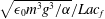 $\sqrt{\unicode[STIX]{x1D716}_{0}m^{3}g^{3}/\unicode[STIX]{x1D6FC}}/Lac_{f}$
and
$\sqrt{\unicode[STIX]{x1D716}_{0}m^{3}g^{3}/\unicode[STIX]{x1D6FC}}/Lac_{f}$
and
 $1/\unicode[STIX]{x1D6FC}a^{2}$
, respectively, whose values are 329.73–404.32 V, 0.66–
$1/\unicode[STIX]{x1D6FC}a^{2}$
, respectively, whose values are 329.73–404.32 V, 0.66–
 $1.80~\unicode[STIX]{x03BC}\text{A}~\text{m}^{-2}$
and 1905–
$1.80~\unicode[STIX]{x03BC}\text{A}~\text{m}^{-2}$
and 1905–
 $860~\text{mm}^{-2}$
for particles of diameter
$860~\text{mm}^{-2}$
for particles of diameter
 $2a=10$
–
$2a=10$
–
 $15~\unicode[STIX]{x03BC}\text{m}$
in the conditions of the experiments of Shoshin & Dreizin (Reference Shoshin and Dreizin2002) (aluminium particles in air,
$15~\unicode[STIX]{x03BC}\text{m}$
in the conditions of the experiments of Shoshin & Dreizin (Reference Shoshin and Dreizin2002) (aluminium particles in air,
 $L=6~\text{mm}$
).
$L=6~\text{mm}$
).
For a given
 $N$
, a solution exists only when the force acting on a particle that bounces off the lower electrode points upwards, i.e. when
$N$
, a solution exists only when the force acting on a particle that bounces off the lower electrode points upwards, i.e. when
 $E(0)>1$
. This condition determines a minimum voltage of the form
$E(0)>1$
. This condition determines a minimum voltage of the form
 $V=V_{min}(N)$
. Upon inversion, this relation determines the stationary number of suspended particles per unit electrode area as a function of the applied voltage for a device with an excess of particles deposited at the lower electrode. The result is shown in figure 3(a) (solid curve), together with the electric current in the gap (dashed curve). Figure 3(b) shows the corresponding distributions of
$V=V_{min}(N)$
. Upon inversion, this relation determines the stationary number of suspended particles per unit electrode area as a function of the applied voltage for a device with an excess of particles deposited at the lower electrode. The result is shown in figure 3(a) (solid curve), together with the electric current in the gap (dashed curve). Figure 3(b) shows the corresponding distributions of
 $n_{\pm }$
and
$n_{\pm }$
and
 $E$
across the gap for various values of
$E$
across the gap for various values of
 $V$
. The number density of positive particles tends to infinity at the lower electrode because
$V$
. The number density of positive particles tends to infinity at the lower electrode because
 $v_{+}$
tends to zero there.
$v_{+}$
tends to zero there.

Figure 3. (a) Maximum dimensionless number of suspended particles per unit electrode area as a function of the dimensionless voltage (solid curve, left-hand side scale), and dimensionless electric current in these conditions (dashed curve, right-hand side scale). The square and circle symbols are experimental results for the maximum number of suspended particles per unit electrode area from Yu & Colver (Reference Yu and Colver1987) and Shoshin & Dreizin (Reference Shoshin and Dreizin2002), respectively. (b) Distributions of positive particles (solid, right-hand side scale), negative particles (dashed) and electric field (dotted) for the maximum value of
 $N$
. Results are shown for
$N$
. Results are shown for
 $V=2$
, 3 and 4, increasing from bottom to top.
$V=2$
, 3 and 4, increasing from bottom to top.
The condition for a particle initially standing on the lower electrode to detach from it is that the electric force acting on the particle be larger than the sum of its weight and the cohesive forces. For a smooth electrode surface, the electric force is (2.2), which amounts to
 $F=(\unicode[STIX]{x1D6FD}/\unicode[STIX]{x1D6FC})E(0)^{2}$
in dimensionless variables. If the cohesive forces can be neglected, this condition reads
$F=(\unicode[STIX]{x1D6FD}/\unicode[STIX]{x1D6FC})E(0)^{2}$
in dimensionless variables. If the cohesive forces can be neglected, this condition reads
 $E(0)>(\unicode[STIX]{x1D6FC}/\unicode[STIX]{x1D6FD})^{1/2}\approx 1.096$
.
$E(0)>(\unicode[STIX]{x1D6FC}/\unicode[STIX]{x1D6FD})^{1/2}\approx 1.096$
.
3.2 Solution for
$N=O(1)$
,
$V=O(\unicode[STIX]{x1D6FC}^{1/2})$


The analysis of the previous section is extended here to large values of
 $V$
to see how the effect of the collisions first comes into play. The Poisson equation in the form (3.7) shows that the effect of the space charge, on its right-hand side, becomes negligible when
$V$
to see how the effect of the collisions first comes into play. The Poisson equation in the form (3.7) shows that the effect of the space charge, on its right-hand side, becomes negligible when
 $V$
(and thus
$V$
(and thus
 $E$
) takes large values keeping
$E$
) takes large values keeping
 $N$
(and thus
$N$
(and thus
 $n_{\pm }$
) of order unity. The electric field in the gap is then uniform at
$n_{\pm }$
) of order unity. The electric field in the gap is then uniform at
 $E=V$
; the charges of the positive and negative particles are opposite,
$E=V$
; the charges of the positive and negative particles are opposite,
 $q_{+}=-q_{-}=V$
, as well as their velocities,
$q_{+}=-q_{-}=V$
, as well as their velocities,
 $v_{+}\approx -v_{-}\approx V^{2}\gg 1$
. The condition of zero flux (3.6) gives
$v_{+}\approx -v_{-}\approx V^{2}\gg 1$
. The condition of zero flux (3.6) gives
 $n_{+}\approx n_{-}$
. The effect of the collisions in the conservation equations for these particles remains negligible because the transport and collision terms increase at the same pace, proportionally to the velocity of the particles.
$n_{+}\approx n_{-}$
. The effect of the collisions in the conservation equations for these particles remains negligible because the transport and collision terms increase at the same pace, proportionally to the velocity of the particles.
Collisions between positive and negative particles generate two other families of particles with smaller charges,
 $q_{0\pm }=\pm \bar{q}_{E}=\pm (\unicode[STIX]{x1D6FE}/\unicode[STIX]{x1D6FC})V$
, and velocities,
$q_{0\pm }=\pm \bar{q}_{E}=\pm (\unicode[STIX]{x1D6FE}/\unicode[STIX]{x1D6FC})V$
, and velocities,
 $v_{0\pm }=\pm (\unicode[STIX]{x1D6FE}/\unicode[STIX]{x1D6FC})V^{2}-1$
. These slow particles contribute little to the total flux. However, their residence time in the gap is larger than that of the particles detaching from the electrodes, which allows the collisions to increase their number densities (denoted
$v_{0\pm }=\pm (\unicode[STIX]{x1D6FE}/\unicode[STIX]{x1D6FC})V^{2}-1$
. These slow particles contribute little to the total flux. However, their residence time in the gap is larger than that of the particles detaching from the electrodes, which allows the collisions to increase their number densities (denoted
 $n_{0\pm }$
in what follows). The conservation equations for the two families of weakly charged particles are
$n_{0\pm }$
in what follows). The conservation equations for the two families of weakly charged particles are
 $$\begin{eqnarray}v_{0\pm }\frac{\text{d}n_{0\pm }}{\text{d}x}\approx \frac{1}{\unicode[STIX]{x1D6FC}}[8\unicode[STIX]{x03C0}V^{2}n_{+}n_{-}-4\unicode[STIX]{x03C0}V^{2}(n_{+}+n_{-})n_{0\pm }]=\frac{8\unicode[STIX]{x03C0}V^{2}}{\unicode[STIX]{x1D6FC}}n_{+}(n_{+}-n_{0\pm }),\end{eqnarray}$$
where the first term on the right-hand side is the rate at which weakly charged particles are generated by collisions of particles with charges
 $q_{+}$
and
$q_{+}$
and
 $q_{-}$
, and the second term is the rate at which they are depleted by their collisions with particles of charge
$q_{-}$
, and the second term is the rate at which they are depleted by their collisions with particles of charge
 $q_{+}$
or
$q_{+}$
or
 $q_{-}$
. The latter collisions lead to yet other families of particles, but these move too fast for collisions to increase their number densities to significant values. The solutions of (3.11) with the boundary conditions
$q_{-}$
. The latter collisions lead to yet other families of particles, but these move too fast for collisions to increase their number densities to significant values. The solutions of (3.11) with the boundary conditions
 $n_{0+}=0$
at
$n_{0+}=0$
at
 $x=0$
and
$x=0$
and
 $n_{0-}=0$
at
$n_{0-}=0$
at
 $x=1$
(assuming that
$x=1$
(assuming that
 $v_{0+}>0$
and
$v_{0+}>0$
and
 $v_{0-}<0$
) are
$v_{0-}<0$
) are
 $n_{0+}=n_{+}\{1-\exp (-8\unicode[STIX]{x03C0}V^{2}n_{+}x/\unicode[STIX]{x1D6FC}v_{0+})\}$
and
$n_{0+}=n_{+}\{1-\exp (-8\unicode[STIX]{x03C0}V^{2}n_{+}x/\unicode[STIX]{x1D6FC}v_{0+})\}$
and
 $n_{0-}=n_{+}\{1-\exp [8\unicode[STIX]{x03C0}V^{2}n_{+}(1-x)/\unicode[STIX]{x1D6FC}v_{0-}]\}$
. These solutions give
$n_{0-}=n_{+}\{1-\exp [8\unicode[STIX]{x03C0}V^{2}n_{+}(1-x)/\unicode[STIX]{x1D6FC}v_{0-}]\}$
. These solutions give
 $n_{0\pm }$
of the order of
$n_{0\pm }$
of the order of
 $n_{+}$
when
$n_{+}$
when
 $V=O(\unicode[STIX]{x1D6FC}^{1/2})$
, so that the exponents cease to be small. Condition (3.3) then reads
$V=O(\unicode[STIX]{x1D6FC}^{1/2})$
, so that the exponents cease to be small. Condition (3.3) then reads
 $\int _{0}^{1}(n_{+}+n_{-}+n_{0+}+n_{0-})\,\text{d}x=N$
and gives
$\int _{0}^{1}(n_{+}+n_{-}+n_{0+}+n_{0-})\,\text{d}x=N$
and gives
 $$\begin{eqnarray}4n_{+}-\frac{\unicode[STIX]{x1D6FC}}{16\unicode[STIX]{x03C0}V^{2}}\left\{v_{0+}\exp \left(-\frac{8\unicode[STIX]{x03C0}V^{2}n_{+}}{\unicode[STIX]{x1D6FC}v_{0+}}\right)-v_{0-}\exp \left(\frac{8\unicode[STIX]{x03C0}V^{2}n_{+}}{\unicode[STIX]{x1D6FC}v_{0-}}\right)\right\}=N,\end{eqnarray}$$
which determines
 $n_{+}$
and completes the solution of the problem.
$n_{+}$
and completes the solution of the problem.
This solution tends to
 $n_{+}=n_{-}=n_{0+}=n_{0-}=N/4$
(except in a thin layers by the electrodes) when
$n_{+}=n_{-}=n_{0+}=n_{0-}=N/4$
(except in a thin layers by the electrodes) when
 $N$
becomes large with
$N$
becomes large with
 $V=O(\unicode[STIX]{x1D6FC}^{1/2})$
. It may be noticed that the effect of the space charge remains negligible in these conditions, despite the fact that each term on the right-hand side of the first equation (3.2) is then large compared to the left-hand side of this equation, because there is nearly complete cancellation of positive and negative charges.
$V=O(\unicode[STIX]{x1D6FC}^{1/2})$
. It may be noticed that the effect of the space charge remains negligible in these conditions, despite the fact that each term on the right-hand side of the first equation (3.2) is then large compared to the left-hand side of this equation, because there is nearly complete cancellation of positive and negative charges.
3.3 Solution for
$N=O(\unicode[STIX]{x1D6FC})$
,
$V=O(\unicode[STIX]{x1D6FC}^{1/2})$


The collision terms of (3.1) are quadratic in the number densities
 $n_{j}$
and become of the order of the convection terms when
$n_{j}$
and become of the order of the convection terms when
 $N$
becomes of order
$N$
becomes of order
 $\unicode[STIX]{x1D6FC}$
. Collisions then populate states of charge different from
$\unicode[STIX]{x1D6FC}$
. Collisions then populate states of charge different from
 $q_{\pm }$
. Numerical solutions of (3.1)–(3.5) show that the number density of particles with charge
$q_{\pm }$
. Numerical solutions of (3.1)–(3.5) show that the number density of particles with charge
 $q_{+}$
decreases, and the number densities of particles with other positive charges increase, when the distance to the lower electrode increases. Similarly, negative charge is transferred from particles with charge
$q_{+}$
decreases, and the number densities of particles with other positive charges increase, when the distance to the lower electrode increases. Similarly, negative charge is transferred from particles with charge
 $q_{-}$
to particles with other negative charges when the distance to the upper electrode increases. The decrease of
$q_{-}$
to particles with other negative charges when the distance to the upper electrode increases. The decrease of
 $n_{\pm }$
with distance to the electrodes is faster when
$n_{\pm }$
with distance to the electrodes is faster when
 $N$
increases.
$N$
increases.
The left- and right-hand sides of (3.7) are of orders
 $V$
and
$V$
and
 $N/V$
. For a given
$N/V$
. For a given
 $N\gg 1$
, the dimensionless voltage
$N\gg 1$
, the dimensionless voltage
 $V$
must be at least of order
$V$
must be at least of order
 $N^{1/2}$
in order for the electric field due to the applied voltage to overcome the field of the space charge. Away from the deposition threshold, the electric field is of order
$N^{1/2}$
in order for the electric field due to the applied voltage to overcome the field of the space charge. Away from the deposition threshold, the electric field is of order
 $V$
everywhere in the gap, leading to
$V$
everywhere in the gap, leading to
 $q_{\pm }=O(V)$
. Particles with charges of this order move very fast, with velocities of
$q_{\pm }=O(V)$
. Particles with charges of this order move very fast, with velocities of
 $O(V^{2})$
, and lead to an electric current of order
$O(V^{2})$
, and lead to an electric current of order
 $NV^{3}$
. The velocity of these particles is little affected by gravity. Gravity is still responsible for the space charge density of order
$NV^{3}$
. The velocity of these particles is little affected by gravity. Gravity is still responsible for the space charge density of order
 $N/V$
left in the gap, but this is small compared to the density of order
$N/V$
left in the gap, but this is small compared to the density of order
 $NV$
that could exist if (3.6) were not satisfied. The right-hand side of (3.7) would be zero in the absence of gravity, and the stationary state would then be symmetric about the centreplane of the gap. This symmetric state is approached when
$NV$
that could exist if (3.6) were not satisfied. The right-hand side of (3.7) would be zero in the absence of gravity, and the stationary state would then be symmetric about the centreplane of the gap. This symmetric state is approached when
 $V\gg N^{1/2}$
, while the asymmetry becomes more pronounced when the voltage is decreased towards the deposition threshold for a given
$V\gg N^{1/2}$
, while the asymmetry becomes more pronounced when the voltage is decreased towards the deposition threshold for a given
 $N$
. Then the density of charge increases in the lower part of the gap, reducing the electric field at the lower electrode and the charge and velocity of the bouncing particles.
$N$
. Then the density of charge increases in the lower part of the gap, reducing the electric field at the lower electrode and the charge and velocity of the bouncing particles.

Figure 4. (a) Charges of the particles detaching from the lower (
 $q_{+}$
, solid curves) and upper (
$q_{+}$
, solid curves) and upper (
 $q_{-}$
, dashed curves) electrodes, from the numerical solution of (3.1)–(3.5), as functions of the voltage for values of the number of particles per unit electrode area
$q_{-}$
, dashed curves) electrodes, from the numerical solution of (3.1)–(3.5), as functions of the voltage for values of the number of particles per unit electrode area
 $N=0$
, 2.07, 8.27, 16.54 and 24.80, increasing as indicated by the arrows. (b) Electric current scaled with
$N=0$
, 2.07, 8.27, 16.54 and 24.80, increasing as indicated by the arrows. (b) Electric current scaled with
 $N$
as a function of the voltage for the same values of
$N$
as a function of the voltage for the same values of
 $N$
. The inset shows the current scaled with
$N$
. The inset shows the current scaled with
 $V^{3}$
as a function of
$V^{3}$
as a function of
 $N$
for
$N$
for
 $V=4.55$
, 6.82 and 9.09, increasing as indicated by the arrow.
$V=4.55$
, 6.82 and 9.09, increasing as indicated by the arrow.
Figure 4 shows some results from the numerical solution of (3.1)–(3.5) with
 $p=77$
. In agreement with the previous estimations,
$p=77$
. In agreement with the previous estimations,
 $q_{+}$
and
$q_{+}$
and
 $q_{-}$
in figure 4(a) increase as
$q_{-}$
in figure 4(a) increase as
 $V$
for large values of this variable, while
$V$
for large values of this variable, while
 $q_{+}$
decreases towards unity at the deposition threshold (the minimum value of
$q_{+}$
decreases towards unity at the deposition threshold (the minimum value of
 $V$
for which a solution with a given
$V$
for which a solution with a given
 $N$
exists). Despite the similarity of figures 2(a) and 4(a), the underlying distributions of charge are very different in the two cases. Figure 4(b) shows
$N$
exists). Despite the similarity of figures 2(a) and 4(a), the underlying distributions of charge are very different in the two cases. Figure 4(b) shows
 $I/N$
as a function of
$I/N$
as a function of
 $V$
. The collapse of the curves when
$V$
. The collapse of the curves when
 $N$
increases shows that the electric current scales with
$N$
increases shows that the electric current scales with
 $N$
for large values of this variable and values of
$N$
for large values of this variable and values of
 $V$
well above the deposition threshold. The inset of figure 4(b) shows that the electric current scales with
$V$
well above the deposition threshold. The inset of figure 4(b) shows that the electric current scales with
 $V^{3}$
in these conditions. Curves for different values of
$V^{3}$
in these conditions. Curves for different values of
 $V$
branch off a common behaviour when the deposition threshold marking the end point of each curve is approached.
$V$
branch off a common behaviour when the deposition threshold marking the end point of each curve is approached.
Near this end point,
 $q_{+}=E(0)=O(1)$
while
$q_{+}=E(0)=O(1)$
while
 $-q_{-}=E(1)=O(V)$
. Particles with positive charges of
$-q_{-}=E(1)=O(V)$
. Particles with positive charges of
 $O(V)$
are generated by collisions in the part of the gap where
$O(V)$
are generated by collisions in the part of the gap where
 $E=O(V)$
and move upwards from the point where they are generated. However, a region of low electric field (
$E=O(V)$
and move upwards from the point where they are generated. However, a region of low electric field (
 $E(x)\ll V$
) and high number density exists around the lower electrode where collisions have no time to affect the distribution of charge (see estimates at the end of this paragraph). In this region, particles with positive charge come from the electrode and move upwards with velocity
$E(x)\ll V$
) and high number density exists around the lower electrode where collisions have no time to affect the distribution of charge (see estimates at the end of this paragraph). In this region, particles with positive charge come from the electrode and move upwards with velocity
 $v_{+}=q_{+}E-1=O(E)$
, while particles with negative charge of
$v_{+}=q_{+}E-1=O(E)$
, while particles with negative charge of
 $O(V)$
enter from above moving downwards with velocities of order
$O(V)$
enter from above moving downwards with velocities of order
 $VE$
. The charge distribution of these particles depends on their dynamics in the bulk of the gap. Let
$VE$
. The charge distribution of these particles depends on their dynamics in the bulk of the gap. Let
 $n_{c_{-}}$
denote their characteristic number density in the region of interest. Condition (3.6) of zero particle flux then gives
$n_{c_{-}}$
denote their characteristic number density in the region of interest. Condition (3.6) of zero particle flux then gives
 $n_{+}v_{+}\sim n_{c_{-}}VE$
, whence
$n_{+}v_{+}\sim n_{c_{-}}VE$
, whence
 $n_{c_{-}}/n_{+}\sim 1/V\ll 1$
. The contributions of positive and negative particles to the electric current are
$n_{c_{-}}/n_{+}\sim 1/V\ll 1$
. The contributions of positive and negative particles to the electric current are
 $I_{+}=q_{+}n_{+}v_{+}\sim n_{+}E$
and
$I_{+}=q_{+}n_{+}v_{+}\sim n_{+}E$
and
 $I_{-}=\sum _{q_{i}<0}q_{i}n_{i}v_{i}\sim n_{c_{-}}V^{2}E\sim n_{+}VE\gg I_{+}$
. Thus most of the particles in this region are slowly moving positive particles, but the electric current is dominated by the less numerous but faster negative particles. Since
$I_{-}=\sum _{q_{i}<0}q_{i}n_{i}v_{i}\sim n_{c_{-}}V^{2}E\sim n_{+}VE\gg I_{+}$
. Thus most of the particles in this region are slowly moving positive particles, but the electric current is dominated by the less numerous but faster negative particles. Since
 $I\approx I_{-}$
is a constant independent of
$I\approx I_{-}$
is a constant independent of
 $x$
, the last balance gives
$x$
, the last balance gives
 $n_{+}\sim I/(VE)$
. Carrying this to the Poisson equation (3.7),
$n_{+}\sim I/(VE)$
. Carrying this to the Poisson equation (3.7),
 $\text{d}E/\text{d}x=(\sum n_{i})/E\approx n_{+}/E\sim I/(VE^{2})$
, which gives
$\text{d}E/\text{d}x=(\sum n_{i})/E\approx n_{+}/E\sim I/(VE^{2})$
, which gives
 $E(x)^{3}-E(0)^{3}\sim (I/V)x$
and thus determines the orders of
$E(x)^{3}-E(0)^{3}\sim (I/V)x$
and thus determines the orders of
 $n_{+}$
,
$n_{+}$
,
 $v_{+}$
and
$v_{+}$
and
 $n_{c_{-}}$
as functions of
$n_{c_{-}}$
as functions of
 $x$
near the lower electrode. Finally, the orders of magnitude of the collision and convection terms for positive particles in this region are
$x$
near the lower electrode. Finally, the orders of magnitude of the collision and convection terms for positive particles in this region are
 $w_{+}/\unicode[STIX]{x1D6FC}\sim VEn_{+}n_{c_{-}}/\unicode[STIX]{x1D6FC}$
and
$w_{+}/\unicode[STIX]{x1D6FC}\sim VEn_{+}n_{c_{-}}/\unicode[STIX]{x1D6FC}$
and
 $\text{d}(n_{+}v_{+})/\text{d}x\sim n_{+}E/x$
, so that the collision–convection ratio is of order
$\text{d}(n_{+}v_{+})/\text{d}x\sim n_{+}E/x$
, so that the collision–convection ratio is of order
 $Vn_{c_{-}}x/\unicode[STIX]{x1D6FC}\sim n_{+}x/\unicode[STIX]{x1D6FC}\sim E^{2}/\unicode[STIX]{x1D6FC}\ll 1$
when
$Vn_{c_{-}}x/\unicode[STIX]{x1D6FC}\sim n_{+}x/\unicode[STIX]{x1D6FC}\sim E^{2}/\unicode[STIX]{x1D6FC}\ll 1$
when
 $N=O(\unicode[STIX]{x1D6FC})$
, because
$N=O(\unicode[STIX]{x1D6FC})$
, because
 $E\ll V\sim N^{1/2}$
. The same estimate holds for negative particles because
$E\ll V\sim N^{1/2}$
. The same estimate holds for negative particles because
 $\sum w_{i}=\sum n_{i}v_{i}=0$
. Collisions are thus negligible near the lower electrode, as was advanced above.
$\sum w_{i}=\sum n_{i}v_{i}=0$
. Collisions are thus negligible near the lower electrode, as was advanced above.
The redistribution of charge in particle collisions due to the electric field in the gap has an important effect on these results. In each collision, the electric field induces equal and opposite charges in the two colliding particles, additional to the mean charge of the pair, and by this means makes for a wide distribution of charge. In the absence of this effect, particles would emerge from collisions with charges equal to the mean charge of the colliding pair, which in the long term leads to a large population of neutral or quasineutral particles.
It has been argued (Myazdrikov Reference Myazdrikov1984; Zhebelev Reference Zhebelev1992) that a stationary solution ceases to exist above a certain value of
 $N$
in the region of decreasing electric current in the inset of figure 4(b) when
$N$
in the region of decreasing electric current in the inset of figure 4(b) when
 $E(0)$
is still larger than unity. The numerical results of this section, which account for the effect of the electric field on the collisions to oppose the concentration of the distribution function about
$E(0)$
is still larger than unity. The numerical results of this section, which account for the effect of the electric field on the collisions to oppose the concentration of the distribution function about
 $q=0$
, do not hint at a maximum
$q=0$
, do not hint at a maximum
 $N$
in these conditions. In fact some of the stationary solutions in figure 4 are for values of
$N$
in these conditions. In fact some of the stationary solutions in figure 4 are for values of
 $N$
higher than the upper bounds proposed by Zhebelev (Reference Zhebelev1992), which are between
$N$
higher than the upper bounds proposed by Zhebelev (Reference Zhebelev1992), which are between
 $\unicode[STIX]{x1D6FC}/4\unicode[STIX]{x03C0}$
and
$\unicode[STIX]{x1D6FC}/4\unicode[STIX]{x03C0}$
and
 $\unicode[STIX]{x1D6FC}/\unicode[STIX]{x03C0}$
in the present dimensionless variables.
$\unicode[STIX]{x1D6FC}/\unicode[STIX]{x03C0}$
in the present dimensionless variables.
The numerical results suggest that a collision-dominated regime develops when
 $N$
becomes large compared to
$N$
becomes large compared to
 $\unicode[STIX]{x1D6FC}$
, with
$\unicode[STIX]{x1D6FC}$
, with
 $V=O(N^{1/2})$
or larger. In this regime, positive and negative contributions to
$V=O(N^{1/2})$
or larger. In this regime, positive and negative contributions to
 $w_{i}/\unicode[STIX]{x1D6FC}$
, each of which is large compared to the convection term in (3.1), nearly balance each other, except in thin layers by the electrodes. This asymptotic regime will not be further discussed here because the results of § 4 suggest that the stationary solution becomes unstable already at smaller values of
$w_{i}/\unicode[STIX]{x1D6FC}$
, each of which is large compared to the convection term in (3.1), nearly balance each other, except in thin layers by the electrodes. This asymptotic regime will not be further discussed here because the results of § 4 suggest that the stationary solution becomes unstable already at smaller values of
 $N$
when the threshold of particle deposition (
$N$
when the threshold of particle deposition (
 $E(0)=1$
) is approached.
$E(0)=1$
) is approached.
3.4 Comparison with experiments
To determine the maximum number of suspended particles (
 $\max (N)$
) as a function of the applied voltage, Colver and coworkers (Colver Reference Colver and Shahinpoor1983; Yu & Colver Reference Yu and Colver1987; Xu Reference Xu2008) carried out experiments in which the number of particles enclosed in a fluidization cell is sequentially increased keeping the voltage constant. These authors measured the number of particles in suspension (by optical means) or the electric current collected at the electrodes, and observed that both magnitudes first increase with the number of particles enclosed and then stabilize at nearly constant values when this number reaches a certain threshold at which a deposit begins forming at the lower electrode. They therefore identified this condition with the sought-for
$\max (N)$
) as a function of the applied voltage, Colver and coworkers (Colver Reference Colver and Shahinpoor1983; Yu & Colver Reference Yu and Colver1987; Xu Reference Xu2008) carried out experiments in which the number of particles enclosed in a fluidization cell is sequentially increased keeping the voltage constant. These authors measured the number of particles in suspension (by optical means) or the electric current collected at the electrodes, and observed that both magnitudes first increase with the number of particles enclosed and then stabilize at nearly constant values when this number reaches a certain threshold at which a deposit begins forming at the lower electrode. They therefore identified this condition with the sought-for
 $\max (N)$
. Yu & Colver (Reference Yu and Colver1987) show a sample result from their experiments in which a mean number density of suspended particles of
$\max (N)$
. Yu & Colver (Reference Yu and Colver1987) show a sample result from their experiments in which a mean number density of suspended particles of
 $8$
–
$8$
–
 $9\times 10^{3}$
cm
$9\times 10^{3}$
cm
 $^{-3}$
was measured at the deposition threshold for
$^{-3}$
was measured at the deposition threshold for
 $96~\unicode[STIX]{x03BC}\text{m}$
copper particles enclosed between disk electrodes 2.63 cm in diameter, spaced a distance
$96~\unicode[STIX]{x03BC}\text{m}$
copper particles enclosed between disk electrodes 2.63 cm in diameter, spaced a distance
 $L=1.1$
cm and subjected to a voltage of 10 kV. The result is recast in dimensionless variables and represented by the square in figure 3(a). It is in good agreement with the theoretical prediction in § 3.1.
$L=1.1$
cm and subjected to a voltage of 10 kV. The result is recast in dimensionless variables and represented by the square in figure 3(a). It is in good agreement with the theoretical prediction in § 3.1.
Shoshin & Dreizin (Reference Shoshin and Dreizin2002) used their analytical model to relate the mean number density of suspended particles to the number density at the upper electrode, which they measured by letting some particles escape through a small orifice at this electrode. These authors present results for 10–
 $14~\unicode[STIX]{x03BC}\text{m}$
aluminium particles in a cell of height
$14~\unicode[STIX]{x03BC}\text{m}$
aluminium particles in a cell of height
 $L=6~\text{mm}$
and voltages of 1.5 and 3 kV. The result for the lower voltage is represented by the circle in figure 3(a). The result for the higher voltage does not fit in the scale of this figure. It gives
$L=6~\text{mm}$
and voltages of 1.5 and 3 kV. The result for the lower voltage is represented by the circle in figure 3(a). The result for the higher voltage does not fit in the scale of this figure. It gives
 $N=47$
for
$N=47$
for
 $V=7.68$
, to be compared with the theoretical prediction
$V=7.68$
, to be compared with the theoretical prediction
 $N=50.1$
at this dimensionless voltage. The fact that the agreement with theoretical results is nearly as good for aluminium as for copper particles suggests that the effect of the electrical resistance of the oxide layer is not important in the experiments of Shoshin & Dreizin (Reference Shoshin and Dreizin2002).
$N=50.1$
at this dimensionless voltage. The fact that the agreement with theoretical results is nearly as good for aluminium as for copper particles suggests that the effect of the electrical resistance of the oxide layer is not important in the experiments of Shoshin & Dreizin (Reference Shoshin and Dreizin2002).

Figure 5. Dimensionless electric current as a function of the dimensionless number of suspended particles per unit electrode area for a constant voltage. The circles show the current measured by Yu & Colver (Reference Yu and Colver1987), scaled with an effective electrode area, for copper particles of
 $96~\unicode[STIX]{x03BC}\text{m}$
enclosed between two horizontal electrode disks of 2.63 cm diameter spaced 1.1 cm and subjected to a voltage difference of 10 kV (
$96~\unicode[STIX]{x03BC}\text{m}$
enclosed between two horizontal electrode disks of 2.63 cm diameter spaced 1.1 cm and subjected to a voltage difference of 10 kV (
 $V=2.93$
in dimensionless variables). Deposition at the lower electrode occurs only when the current levels off. The dashed curve is the theoretical prediction for this case. The rightmost point of this curve marks the deposition threshold.
$V=2.93$
in dimensionless variables). Deposition at the lower electrode occurs only when the current levels off. The dashed curve is the theoretical prediction for this case. The rightmost point of this curve marks the deposition threshold.
In principle, the experiments of Colver and coworkers offer a possibility of testing the theoretical predictions also in the absence of deposition, as they give results for cases when all the enclosed particles are in suspension. However, the idealized unidimensional state hypothesized above is not realized in these experiments. The electrodes used were disks of reduced size, either open at the edge or closed by a dielectric cylindrical wall, and perhaps more importantly, the cell was of the guard-ring capacitor type, with a central orifice at the upper disk. For these reasons, the density of electric current was not uniform on the electrodes, and comparison with theoretical unidimensional predictions requires introducing an effective electrode area smaller than the area of the disks by a certain unknown factor. Figure 2 of Yu & Colver (Reference Yu and Colver1987) shows the measured current as a function of the mean number density for the conditions mentioned at the beginning of this section. The results are recast in dimensionless variables and shown in figure 5 together with the theoretical prediction in § 3.1 (dashed curve). The good agreement between experimental and theoretical results has been obtained by multiplying the area of the electrode disks by an arbitrary factor of 0.7 and adjusting the mean number density accordingly. However, the shapes of the experimental and theoretical curves at the left of the maximum of the latter agree irrespective of this factor.
Similar experiments were performed by Xu (Reference Xu2008) with particles and cells of various materials, using different techniques to measure the number of particles in suspension and the electric current. The results agree with the theoretical prediction up to the uncertainty introduced by the arbitrary surface scale factor.
A noteworthy feature of the theoretical prediction is the decrease of the electric current with increasing
 $N$
in a range of values of this variable near the deposition threshold
$N$
in a range of values of this variable near the deposition threshold
 $E(0)=1$
(the end point of the dashed curve in figure 5); see also the inset of figure 4(b). The increase of the number of charged particles is outweighed in this region by the decrease of their charge accompanying the decrease of the electric field at the lower electrode. The decrease of the current was noted by Xu (Reference Xu2008) in some of his experiments, though it does not seem to have been taken into account in the determination of the deposition threshold. This author also notes that the suspension may become unstable before deposition occurs. This observation is in line with the results of the stability analysis of the following section.
$E(0)=1$
(the end point of the dashed curve in figure 5); see also the inset of figure 4(b). The increase of the number of charged particles is outweighed in this region by the decrease of their charge accompanying the decrease of the electric field at the lower electrode. The decrease of the current was noted by Xu (Reference Xu2008) in some of his experiments, though it does not seem to have been taken into account in the determination of the deposition threshold. This author also notes that the suspension may become unstable before deposition occurs. This observation is in line with the results of the stability analysis of the following section.
4 Time-dependent flow
The transient evolution of the aerosol is analysed for low particle densities, for which the effect of interparticle collisions is negligible and each particle conserves its charge in its journey across the gap, equal to the charge with which it last detached from an electrode. This charge is determined by the field at the electrode at the moment of detachment, which is no longer a constant but depends on position on the electrode and time. The Eulerian formulation of § 3.1 can be extended to describe a transient. The governing equations are
 $$\begin{eqnarray}\frac{\unicode[STIX]{x2202}n_{\pm }}{\unicode[STIX]{x2202}t}+\unicode[STIX]{x1D735}\boldsymbol{\cdot }(n_{\pm }\boldsymbol{v}_{\pm })=0,\quad \frac{\unicode[STIX]{x2202}q_{\pm }}{\unicode[STIX]{x2202}t}+\boldsymbol{v}_{\pm }\boldsymbol{\cdot }\unicode[STIX]{x1D735}q_{\pm }=0,\quad \boldsymbol{v}_{\pm }=\boldsymbol{v}_{g}+q_{\pm }\boldsymbol{E}-\hat{\boldsymbol{\imath }},\end{eqnarray}$$
 $$\begin{eqnarray}\unicode[STIX]{x1D6FB}^{2}\unicode[STIX]{x1D711}=-(n_{+}q_{+}+n_{-}q_{-}),\quad \boldsymbol{E}=-\unicode[STIX]{x1D735}\unicode[STIX]{x1D711},\end{eqnarray}$$
 $$\begin{eqnarray}\unicode[STIX]{x1D735}\boldsymbol{\cdot }\boldsymbol{v}_{g}=0,\quad R\frac{\text{D}\boldsymbol{v}_{g}}{\text{D}t}=-\unicode[STIX]{x1D735}p_{g}+\unicode[STIX]{x1D6FB}^{2}\boldsymbol{v}_{g}+\frac{1}{\unicode[STIX]{x1D6FC}\widetilde{a}}[n_{+}(q_{+}\boldsymbol{E}-\hat{\boldsymbol{\imath }})+n_{-}(q_{-}\boldsymbol{E}-\hat{\boldsymbol{\imath }})],\end{eqnarray}$$
with the boundary conditions (
 $E=|\boldsymbol{E}|$
)
$E=|\boldsymbol{E}|$
)
 $$\begin{eqnarray}\left.\begin{array}{@{}c@{}}\displaystyle x=0:n_{+}\boldsymbol{v}_{+}=-n_{-}\boldsymbol{v}_{-},\quad q_{+}=E,\quad \unicode[STIX]{x1D711}=0,\quad \boldsymbol{v}_{g}=0,\\ \displaystyle x=1:n_{-}\boldsymbol{v}_{-}=-n_{+}\boldsymbol{v}_{+},\quad q_{-}=-E,\quad \unicode[STIX]{x1D711}=-V,\quad \boldsymbol{v}_{g}=0.\end{array}\right\}\end{eqnarray}$$
The conservation equations for
 $n_{\pm }$
in (4.1) together with the first boundary condition at each electrode in (4.4) imply that the number of suspended particles is conserved:
$n_{\pm }$
in (4.1) together with the first boundary condition at each electrode in (4.4) imply that the number of suspended particles is conserved:
 $$\begin{eqnarray}\int (n_{+}+n_{-})\,\text{d}\boldsymbol{x}=N\widetilde{A},\end{eqnarray}$$
where the number of suspended particles per unit electrode area,
 $N$
, is determined by the initial condition. This need not be the case for non-stationary systems with an excess of particles deposited at the lower electrode. A modified boundary condition at the lower electrode that allows for a variable number of suspended particles will be introduced in the linear stability analysis of § 4.1. Extension of this condition to more general cases would require a model of the rate of particle deposition/resuspension that is beyond the scope of this work.
$N$
, is determined by the initial condition. This need not be the case for non-stationary systems with an excess of particles deposited at the lower electrode. A modified boundary condition at the lower electrode that allows for a variable number of suspended particles will be introduced in the linear stability analysis of § 4.1. Extension of this condition to more general cases would require a model of the rate of particle deposition/resuspension that is beyond the scope of this work.
4.1 Linear stability
Linearizing (4.1)–(4.4) for small perturbations of the form
 $$\begin{eqnarray}\unicode[STIX]{x1D6FF}n_{+}=\text{Re}\{\hat{n}_{+}(x)\exp [\text{i}(k_{y}y+k_{z}z)+st]\},\end{eqnarray}$$
and similarly for other variables, an eigenvalue problem is obtained whose eigenvalues are of the form
 $s=s(k;N,V,R,\widetilde{a})$
with
$s=s(k;N,V,R,\widetilde{a})$
with
 $k=(k_{y}^{2}+k_{z}^{2})^{1/2}$
. The eigenvalue with largest real part is shown in figure 6 as a function of
$k=(k_{y}^{2}+k_{z}^{2})^{1/2}$
. The eigenvalue with largest real part is shown in figure 6 as a function of
 $k$
for
$k$
for
 $N=2.067$
,
$N=2.067$
,
 $R=12.92$
,
$R=12.92$
,
 $\widetilde{a}=8.84\times 10^{-5}$
(particles of
$\widetilde{a}=8.84\times 10^{-5}$
(particles of
 $20~\unicode[STIX]{x03BC}\text{m}$
in the experiments of Shoshin & Dreizin), and various values of
$20~\unicode[STIX]{x03BC}\text{m}$
in the experiments of Shoshin & Dreizin), and various values of
 $V$
.
$V$
.

Figure 6. Growth rate (solid curves) and oscillation frequency (dashed curves, right-hand side scale) for the eigenvalue with largest real part as functions of the wavenumber for
 $N=2.067$
,
$N=2.067$
,
 $R=12.92$
,
$R=12.92$
,
 $\widetilde{a}=8.84\times 10^{-5}$
and four values of the dimensionless voltage,
$\widetilde{a}=8.84\times 10^{-5}$
and four values of the dimensionless voltage,
 $V=2.05$
, 2.11, 2.18 and 2.25, increasing as indicated by the arrows.
$V=2.05$
, 2.11, 2.18 and 2.25, increasing as indicated by the arrows.
As can be seen, the stationary state becomes unstable when the voltage
 $V$
decreases below a certain value. This instability is oscillatory (
$V$
decreases below a certain value. This instability is oscillatory (
 $\text{Im}(s)\neq 0$
) and extends to a range of wavenumbers that increases with decreasing
$\text{Im}(s)\neq 0$
) and extends to a range of wavenumbers that increases with decreasing
 $V$
. A second range of unstable wavenumbers appears around
$V$
. A second range of unstable wavenumbers appears around
 $k=0$
when
$k=0$
when
 $V$
is further decreased. The first of these instabilities is hydrodynamic; it disappears when the motion of the gas induced by the drag of the particles is ignored (formally, in the limit
$V$
is further decreased. The first of these instabilities is hydrodynamic; it disappears when the motion of the gas induced by the drag of the particles is ignored (formally, in the limit
 $\unicode[STIX]{x1D6FC}\rightarrow \infty$
). The second instability remains in this limit. It is an instability of the stationary distribution of charge associated to the large concentration of positive particles that appears around the lower electrode when
$\unicode[STIX]{x1D6FC}\rightarrow \infty$
). The second instability remains in this limit. It is an instability of the stationary distribution of charge associated to the large concentration of positive particles that appears around the lower electrode when
 $V$
decreases.
$V$
decreases.
Inspection of the eigenmodes shows that the perturbations with largest growth rate develop near the lower electrode, where various excesses and defects of positive particles stack vertically. Apparently, in a certain range of wavenumbers, a perturbation that increases the density of positive charge around a point of the lower electrode locally increases the force acting on the gas and induces a vertical flow that helps carrying the excess of charge away from the electrode. This increases the amplitude of the perturbation by initiating an electrohydrodynamic plume.
In the absence of gas motion, the excess of charge would stay longer near the electrode, and the perturbation of the electric field that it induces at the electrode would decrease the charge of the particles that detach later. In these conditions, repetition of this process with alternating excesses and defects of charge may cause the stacks mentioned above, which only become unstable when the voltage is further decreased.

Figure 7. Stability limit in the (
 $N$
,
$N$
,
 $V$
) plane for
$V$
) plane for
 $R=12.92$
,
$R=12.92$
,
 $\widetilde{a}=8.84\times 10^{-5}$
(lower solid curve) and
$\widetilde{a}=8.84\times 10^{-5}$
(lower solid curve) and
 $R=29.07$
,
$R=29.07$
,
 $\widetilde{a}=1.33\times 10^{-4}$
(upper solid curve). The dashed curve shows the deposition threshold
$\widetilde{a}=1.33\times 10^{-4}$
(upper solid curve). The dashed curve shows the deposition threshold
 $E(0)=1$
(the solid curve in figure 3
a). In each case, the stationary state is linearly stable below the solid curve and particle deposition on the lower electrode occurs above the dashed curve.
$E(0)=1$
(the solid curve in figure 3
a). In each case, the stationary state is linearly stable below the solid curve and particle deposition on the lower electrode occurs above the dashed curve.
Figure 7 shows the stability limit in the (
 $N$
,
$N$
,
 $V$
) plane for
$V$
) plane for
 $R=12.92$
,
$R=12.92$
,
 $\widetilde{a}=8.84\times 10^{-5}$
(lower solid curve), and
$\widetilde{a}=8.84\times 10^{-5}$
(lower solid curve), and
 $R=29.07$
,
$R=29.07$
,
 $\widetilde{a}=1.33\times 10^{-4}$
(upper solid curve), which correspond to particles of size
$\widetilde{a}=1.33\times 10^{-4}$
(upper solid curve), which correspond to particles of size
 $20~\unicode[STIX]{x03BC}\text{m}$
and
$20~\unicode[STIX]{x03BC}\text{m}$
and
 $30~\unicode[STIX]{x03BC}\text{m}$
, respectively, in the conditions of the experiments of Shoshin & Dreizin (Reference Shoshin and Dreizin2002). The dashed curve in this figure shows the deposition threshold
$30~\unicode[STIX]{x03BC}\text{m}$
, respectively, in the conditions of the experiments of Shoshin & Dreizin (Reference Shoshin and Dreizin2002). The dashed curve in this figure shows the deposition threshold
 $E(0)=1$
. In each case, the stationary state is unstable in the wedge between the solid and the dashed curve. The kink of the upper solid curve reflects a change in the dominant instability. For values of
$E(0)=1$
. In each case, the stationary state is unstable in the wedge between the solid and the dashed curve. The kink of the upper solid curve reflects a change in the dominant instability. For values of
 $N$
above 0.9, the first instability to appear when
$N$
above 0.9, the first instability to appear when
 $V$
is decreased is that with
$V$
is decreased is that with
 $k=0$
.
$k=0$
.
A large number density of particles near the lower electrode is a necessary condition for instability, and this condition is realized near the dashed curve in figure 7. On this curve deposition begins to occur and the number density of positive particles diverges at the lower electrode. The region of instability can be approached either by decreasing the voltage at constant
 $N$
or by increasing
$N$
or by increasing
 $N$
at constant voltage, but both ways amount to approaching the threshold of particle deposition and thus increasing the maximum number density.
$N$
at constant voltage, but both ways amount to approaching the threshold of particle deposition and thus increasing the maximum number density.
A modified eigenvalue problem has also been considered to mimic the presence of deposited particles at the lower electrode, which allows for a variable number of suspended particles during the development of the instability. For this purpose, the first boundary condition (4.4) at the lower electrode is replaced by the condition that the electric field be constant at this electrode. Strictly, this field should be equal to unity, but the value
 $1+\unicode[STIX]{x1D702}$
with
$1+\unicode[STIX]{x1D702}$
with
 $\unicode[STIX]{x1D702}$
as small as
$\unicode[STIX]{x1D702}$
as small as
 $10^{-3}$
has been used to avoid the divergence of the stationary number density of positive particles. Numerical tests show that the effect of a small
$10^{-3}$
has been used to avoid the divergence of the stationary number density of positive particles. Numerical tests show that the effect of a small
 $\unicode[STIX]{x1D702}$
on the eigenvalue with largest real part is negligible. Solution of this eigenvalue problem shows that the modified boundary condition has only a small effect on the hydrodynamic instability, although it suppresses the second instability discussed above, which was due to the variation of the electric field at the lower electrode caused by the perturbation of the space charge above this electrode. On (essentially) the dashed curve in figure 7, the stationary solution becomes unstable when
$\unicode[STIX]{x1D702}$
on the eigenvalue with largest real part is negligible. Solution of this eigenvalue problem shows that the modified boundary condition has only a small effect on the hydrodynamic instability, although it suppresses the second instability discussed above, which was due to the variation of the electric field at the lower electrode caused by the perturbation of the space charge above this electrode. On (essentially) the dashed curve in figure 7, the stationary solution becomes unstable when
 $N$
becomes larger than approximately 0.185 (for which
$N$
becomes larger than approximately 0.185 (for which
 $V\approx 1.115$
; the black circle in the figure), in agreement with the results of the analysis for a constant number of suspended particles. It seems thus that particle deposition and resuspension does not suppress the instability that appeared already above the deposition threshold, when these processes did not occur.
$V\approx 1.115$
; the black circle in the figure), in agreement with the results of the analysis for a constant number of suspended particles. It seems thus that particle deposition and resuspension does not suppress the instability that appeared already above the deposition threshold, when these processes did not occur.
Similarly, the instability is not expected to disappear when the number of particles per unit electrode area increases to values of
 $O(\unicode[STIX]{x1D6FC})$
and interparticle collisions come into play.
$O(\unicode[STIX]{x1D6FC})$
and interparticle collisions come into play.
4.2 Nonlinear transients
The dynamics of large-amplitude perturbations in systems without deposited particles is computed with a combination of an Eulerian, mesoscale description of the gas and the electric field (Williams Reference Williams1985) and a Lagrangian, particle-in-cell description of the particles (Hockney & Eastwood Reference Hockney and Eastwood1988; Birdsall & Langdon Reference Birdsall and Langdon1991). Starting from a random initial distribution, the positions of the particles change according to
 $$\begin{eqnarray}\frac{\text{d}\boldsymbol{x}_{i}}{\text{d}t}=\boldsymbol{v}_{gi}+q_{i}\boldsymbol{E}_{i}-\hat{\boldsymbol{\imath }}\quad \text{for }i=1,\ldots ,N_{p},\end{eqnarray}$$
where
 $N_{p}$
is the number of particles in the gap, equal to
$N_{p}$
is the number of particles in the gap, equal to
 $N\widetilde{A}/\unicode[STIX]{x1D6FC}(6\unicode[STIX]{x03C0}\widetilde{a})^{2}$
in terms of the dimensionless variables of § 2, and
$N\widetilde{A}/\unicode[STIX]{x1D6FC}(6\unicode[STIX]{x03C0}\widetilde{a})^{2}$
in terms of the dimensionless variables of § 2, and
 $\boldsymbol{v}_{gi}$
and
$\boldsymbol{v}_{gi}$
and
 $\boldsymbol{E}_{i}$
are the gas velocity and electric field at the position
$\boldsymbol{E}_{i}$
are the gas velocity and electric field at the position
 $\boldsymbol{x}_{i}$
of particle
$\boldsymbol{x}_{i}$
of particle
 $i$
.
$i$
.
When a particle hits the lower (respectively upper) electrode, it is replaced by a particle injected at the same electrode point with charge
 $q_{+}=E$
(respectively
$q_{+}=E$
(respectively
 $q_{-}=-E$
), where
$q_{-}=-E$
), where
 $E$
is the local instantaneous value of the electric field. Therefore the total number of suspended particles is conserved as far as this process can be carried out; i.e., when
$E$
is the local instantaneous value of the electric field. Therefore the total number of suspended particles is conserved as far as this process can be carried out; i.e., when
 $q_{+}E-1>0$
(respectively
$q_{+}E-1>0$
(respectively
 $q_{-}E-1<0$
).
$q_{-}E-1<0$
).
Only two-dimensional simulations have been done, in which the variables depend on a single horizontal coordinate (
 $y$
) in addition to the vertical coordinate
$y$
) in addition to the vertical coordinate
 $x$
. In these simulations, each particle can be understood as an array of identical particles equispaced in the third direction. Periodicity conditions are used in
$x$
. In these simulations, each particle can be understood as an array of identical particles equispaced in the third direction. Periodicity conditions are used in
 $y$
. The parameter
$y$
. The parameter
 $\widetilde{A}$
in (2.20) is here the ratio of the
$\widetilde{A}$
in (2.20) is here the ratio of the
 $y$
-period to the interelectrode distance.
$y$
-period to the interelectrode distance.
The electric potential and the velocity and pressure of the gas are determined by (2.15) and (2.16) with the relevant boundary conditions in (2.18) and (2.19). The charge and force densities appearing in these equations are
 $$\begin{eqnarray}\unicode[STIX]{x1D70C}_{e}=\frac{(6\unicode[STIX]{x03C0}\widetilde{a})^{2}\unicode[STIX]{x1D6FC}}{\unicode[STIX]{x1D6FF}{\mathcal{V}}}\sum q_{i}\quad \text{and}\quad \boldsymbol{F}=\frac{(6\unicode[STIX]{x03C0})^{2}\widetilde{a}}{\unicode[STIX]{x1D6FF}{\mathcal{V}}}\sum (q_{i}\boldsymbol{E}-\hat{\boldsymbol{\imath }})\end{eqnarray}$$
in the variables used in this section. Here the sums are over the particles present in a control volume
 $\unicode[STIX]{x1D6FF}{\mathcal{V}}$
centred at point
$\unicode[STIX]{x1D6FF}{\mathcal{V}}$
centred at point
 $\boldsymbol{x}$
at time
$\boldsymbol{x}$
at time
 $t$
, and the factors
$t$
, and the factors
 $(6\unicode[STIX]{x03C0}\widetilde{a})^{2}\unicode[STIX]{x1D6FC}$
and
$(6\unicode[STIX]{x03C0}\widetilde{a})^{2}\unicode[STIX]{x1D6FC}$
and
 $(6\unicode[STIX]{x03C0})^{2}\widetilde{a}$
are a consequence of the non-dimensionalization.
$(6\unicode[STIX]{x03C0})^{2}\widetilde{a}$
are a consequence of the non-dimensionalization.
The numerical treatment of this problem is fairly standard. Equations (2.16) are rewritten in the equivalent stream function–vorticity formulation. These equations are discretized together with the Poisson equation (2.15) using second-order finite differences in
 $x$
and spectral collocation in
$x$
and spectral collocation in
 $y$
. They are marched in time along with (4.7) using second-order methods. A Crank–Nicolson method with a standard preconditioned biconjugate gradient is used for the viscous term, and an Adams–Bashforth method is used for the rest. Numerical tests show that grid independence is achieved with a non-uniform
$y$
. They are marched in time along with (4.7) using second-order methods. A Crank–Nicolson method with a standard preconditioned biconjugate gradient is used for the viscous term, and an Adams–Bashforth method is used for the rest. Numerical tests show that grid independence is achieved with a non-uniform
 $x$
-grid of 120 points, finer around the lower electrode, and 512 Fourier modes in
$x$
-grid of 120 points, finer around the lower electrode, and 512 Fourier modes in
 $y$
(for
$y$
(for
 $\tilde{A}=6$
). A dimensionless time step of
$\tilde{A}=6$
). A dimensionless time step of
 $5\times 10^{-5}$
has been used.
$5\times 10^{-5}$
has been used.
The hybrid Eulerian/Lagrangian character of the simulation requires that the velocity of the gas and the electric field be evaluated at the positions of the particles, in (4.7), and that the charge and force densities in (4.8) be evaluated in terms of the charges of individual particles and the forces they exert on the gas. For this purpose, the gas velocity and the electric field are linearly interpolated to the positions of the particles in each grid cell, and the charges and forces of the particles on the gas are projected onto the grid using a linear weighting particle-in-cell method (Birdsall & Langdon Reference Birdsall and Langdon1991) to evaluate (4.8). The volumes of the grid cells are used for
 $\unicode[STIX]{x1D6FF}{\mathcal{V}}$
.
$\unicode[STIX]{x1D6FF}{\mathcal{V}}$
.
To further reduce the numerical burden in cases when the number of particles in the gap is very large, particles are grouped in superparticles. Each superparticle obeys the same (4.7) as individual particles, but it counts for as many particles as it represents in the sums (4.8). The number of particles per superparticle is a free parameter of the method; see Hockney & Eastwood (Reference Hockney and Eastwood1988) and Birdsall & Langdon (Reference Birdsall and Langdon1991). In the computations discussed below, which require
 $N_{p}=215\,820$
, this number is 5. Numerical tests consisting of sample runs in which the particles are treated individually show that this grouping does not degrade the accuracy of the results.
$N_{p}=215\,820$
, this number is 5. Numerical tests consisting of sample runs in which the particles are treated individually show that this grouping does not degrade the accuracy of the results.
The code developed has been validated on related problems for which results of Eulerian simulations are available for comparison; see Higuera (Reference Higuera2016) and Higuera & Tejera (Reference Higuera and Tejera2017).
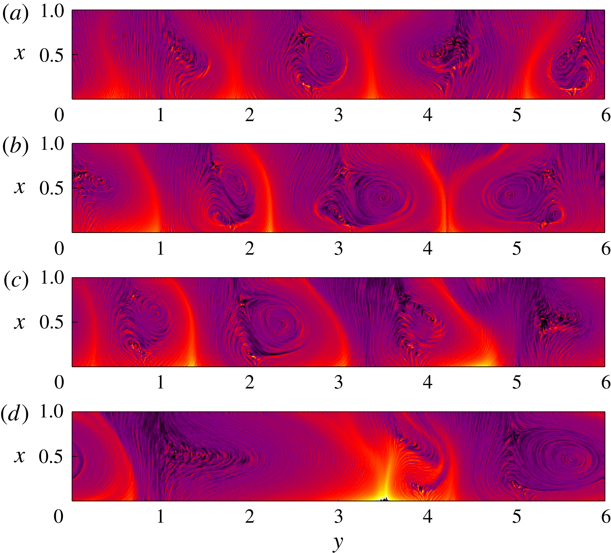


Figure 8 shows some snapshots of the number density of positive particles,
 $$\begin{eqnarray}n_{+}=\frac{(6\unicode[STIX]{x03C0}\widetilde{a})^{2}\unicode[STIX]{x1D6FC}}{\unicode[STIX]{x1D6FF}{\mathcal{V}}}\sum 1^{+},\end{eqnarray}$$
computed for
 $N=2.067$
,
$N=2.067$
,
 $V=2.14$
,
$V=2.14$
,
 $R=12.92$
and
$R=12.92$
and
 $\widetilde{a}=8.84\times 10^{-5}$
in a domain of width
$\widetilde{a}=8.84\times 10^{-5}$
in a domain of width
 $\widetilde{A}=6$
. Here the sum extends to particles with positive charge (coming from the lower electrode) in
$\widetilde{A}=6$
. Here the sum extends to particles with positive charge (coming from the lower electrode) in
 $\unicode[STIX]{x1D6FF}{\mathcal{V}}$
. To reduce the noise intrinsic to the particle method, the variable shown in figure 8 is averaged over 1000 time steps, spanning a dimensionless time 0.05. The most salient events of the history displayed by the simulation from which this figure is extracted are briefly described here. Some of these events appear also in other simulations, although the history itself changes from case to case.
$\unicode[STIX]{x1D6FF}{\mathcal{V}}$
. To reduce the noise intrinsic to the particle method, the variable shown in figure 8 is averaged over 1000 time steps, spanning a dimensionless time 0.05. The most salient events of the history displayed by the simulation from which this figure is extracted are briefly described here. Some of these events appear also in other simulations, although the history itself changes from case to case.
In an initial stage, a number of structures with an average spacing of the order of the wavelength of the most unstable perturbations emerge from the background of noise and fall back to it, sometimes after two of these structures merge. By
 $t=1.225$
(figure 8
a) four plumes are clearly established in the computational domain. The three at the left-hand side of the figure drift towards the right, and the rightmost plume drifts towards the left. Counter-rotating vortices are visible at the lee side of some of these plumes and move with them.
$t=1.225$
(figure 8
a) four plumes are clearly established in the computational domain. The three at the left-hand side of the figure drift towards the right, and the rightmost plume drifts towards the left. Counter-rotating vortices are visible at the lee side of some of these plumes and move with them.
At approximately
 $t=1.825$
(figure 8
b), the two plumes at the right of the figure, which were drifting in opposite directions, collide and merge. The space at the right of the emerging plume, which due to the periodicity condition extends to the leftmost plume in the figure, is wider than the spaces between other plumes and contains two couples of vortices, one at each side of figure 8(b).
$t=1.825$
(figure 8
b), the two plumes at the right of the figure, which were drifting in opposite directions, collide and merge. The space at the right of the emerging plume, which due to the periodicity condition extends to the leftmost plume in the figure, is wider than the spaces between other plumes and contains two couples of vortices, one at each side of figure 8(b).
A new plume appears in this wide space at approximately
 $t=2.525$
(figure 8
c; plume at the left-hand side). The four plumes now present in the domain drift towards the right, together with their vortex structures. However, the two plumes at the left drift faster than the other two. They distort and overtake the vortices in the intervening spaces and, one after the other, collide with the plume that was third from the left in figure 8(c), merging with it. At
$t=2.525$
(figure 8
c; plume at the left-hand side). The four plumes now present in the domain drift towards the right, together with their vortex structures. However, the two plumes at the left drift faster than the other two. They distort and overtake the vortices in the intervening spaces and, one after the other, collide with the plume that was third from the left in figure 8(c), merging with it. At
 $t=4.225$
(figure 8
d) a strong plume has just been generated by this double merger. The rightmost plume in figure 8(c), which was not involved in the process, is now at the left-hand side of figure 8(d). Finally, after some reordering of the vortices at the lee side of the rightmost plume in figure 8(d), the two plumes drift at approximately the same velocity without further collisions.
$t=4.225$
(figure 8
d) a strong plume has just been generated by this double merger. The rightmost plume in figure 8(c), which was not involved in the process, is now at the left-hand side of figure 8(d). Finally, after some reordering of the vortices at the lee side of the rightmost plume in figure 8(d), the two plumes drift at approximately the same velocity without further collisions.
The time-averaged electric current collected at the electrodes in this simulation is 46.84 per unit electrode area, with an r.m.s. value of only 3.31. This average current density is to be compared with the current density of the stationary state for the same values of
 $N$
and
$N$
and
 $V$
, which is 18.32. The transient structures significantly increase the current causing only small fluctuations in the external circuit. They can go unnoticed if current fluctuations are used as an indicator. The fluctuations of the number density of particles at the upper electrode, which could be relevant to characterize the spray issuing from a small orifice in this electrode, are also small.
$V$
, which is 18.32. The transient structures significantly increase the current causing only small fluctuations in the external circuit. They can go unnoticed if current fluctuations are used as an indicator. The fluctuations of the number density of particles at the upper electrode, which could be relevant to characterize the spray issuing from a small orifice in this electrode, are also small.
An additional computation in a domain twice as wide (
 $\widetilde{A}=12$
) has been carried out to ascertain if the final state with only two plumes is an effect of the artificial periodicity condition. In this case, after a number of events, three plumes are left in the computational domain. It seems therefore that collisions between these structures cease in the two-dimensional simulations when the mean spacing between them becomes larger than 3–4 times the depth of the gap. An extensive investigation of the long-term evolution of the system is beyond the scope of this work.
$\widetilde{A}=12$
) has been carried out to ascertain if the final state with only two plumes is an effect of the artificial periodicity condition. In this case, after a number of events, three plumes are left in the computational domain. It seems therefore that collisions between these structures cease in the two-dimensional simulations when the mean spacing between them becomes larger than 3–4 times the depth of the gap. An extensive investigation of the long-term evolution of the system is beyond the scope of this work.
The through gas flow required to push the suspended particles out of the interelectrode gap has not been accounted for. Some possible effects of this flow are briefly commented upon here to close this section. The flow is expected to affect the suspension when its velocity is of the order of the velocities of the particles due to the electric forces. A vertical upward gas flow injected through the electrodes could be a rough model of the mesh electrode configuration of Kim (Reference Kim1989), though detailed modelling of this device would be far too complex. The vertical flow would push the particles upwards, increasing the maximum number of particles that can be suspended for a given voltage. For given values of
 $N$
and
$N$
and
 $V$
, the flow would decrease the number density of particles near the lower electrode, and thus should push the stability limit in figure 7 to larger values of these parameters. A radially converging gas flow carrying the suspension towards an outlet orifice at the centre of the upper electrode (Shoshin & Dreizin Reference Shoshin and Dreizin2002) leads to a velocity that increases as the inverse of the distance to the outlet while this distance is large compared to the interelectrode distance. In the absence of viscosity, the flow in this region would merely transport the particles radially. However, vorticity generation at the electrode surfaces can very much complicate this picture.
$V$
, the flow would decrease the number density of particles near the lower electrode, and thus should push the stability limit in figure 7 to larger values of these parameters. A radially converging gas flow carrying the suspension towards an outlet orifice at the centre of the upper electrode (Shoshin & Dreizin Reference Shoshin and Dreizin2002) leads to a velocity that increases as the inverse of the distance to the outlet while this distance is large compared to the interelectrode distance. In the absence of viscosity, the flow in this region would merely transport the particles radially. However, vorticity generation at the electrode surfaces can very much complicate this picture.
4.3 Effect of the particle inertia
The effect of the inertia of the particles has been left out up to this point on the basis of the estimations of § 2. It can be taken into account replacing (4.7) by
 $$\begin{eqnarray}St\frac{\text{d}\boldsymbol{v}_{i}}{\text{d}t}=q_{i}\boldsymbol{E}_{i}-\hat{\boldsymbol{\imath }}-(\boldsymbol{v}_{i}-\boldsymbol{v}_{gi})\quad \text{and}\quad \frac{\text{d}\boldsymbol{x}_{i}}{\text{d}t}=\boldsymbol{v}_{i}\quad \text{for }i=1,\ldots ,N_{p},\end{eqnarray}$$
where
 $St=m^{2}g/c_{f}^{2}L$
; replacing
$St=m^{2}g/c_{f}^{2}L$
; replacing
 $\boldsymbol{v}_{+}=q_{+}\boldsymbol{E}-\hat{\boldsymbol{\imath }}$
in the boundary condition at
$\boldsymbol{v}_{+}=q_{+}\boldsymbol{E}-\hat{\boldsymbol{\imath }}$
in the boundary condition at
 $x=0$
by
$x=0$
by
 $\boldsymbol{v}_{+}\boldsymbol{\cdot }\hat{\boldsymbol{\imath }}=-r\boldsymbol{v}_{-}\boldsymbol{\cdot }\hat{\boldsymbol{\imath }}$
and
$\boldsymbol{v}_{+}\boldsymbol{\cdot }\hat{\boldsymbol{\imath }}=-r\boldsymbol{v}_{-}\boldsymbol{\cdot }\hat{\boldsymbol{\imath }}$
and
 $\boldsymbol{v}_{+}\times \hat{\boldsymbol{\imath }}=\boldsymbol{v}_{-}\times \hat{\boldsymbol{\imath }}$
, and similarly
$\boldsymbol{v}_{+}\times \hat{\boldsymbol{\imath }}=\boldsymbol{v}_{-}\times \hat{\boldsymbol{\imath }}$
, and similarly
 $\boldsymbol{v}_{-}\boldsymbol{\cdot }\hat{\boldsymbol{\imath }}=-r\boldsymbol{v}_{+}\boldsymbol{\cdot }\hat{\boldsymbol{\imath }}$
and
$\boldsymbol{v}_{-}\boldsymbol{\cdot }\hat{\boldsymbol{\imath }}=-r\boldsymbol{v}_{+}\boldsymbol{\cdot }\hat{\boldsymbol{\imath }}$
and
 $\boldsymbol{v}_{-}\times \hat{\boldsymbol{\imath }}=\boldsymbol{v}_{+}\times \hat{\boldsymbol{\imath }}$
at
$\boldsymbol{v}_{-}\times \hat{\boldsymbol{\imath }}=\boldsymbol{v}_{+}\times \hat{\boldsymbol{\imath }}$
at
 $x=1$
, where
$x=1$
, where
 $r$
is a coefficient of restitution in
$r$
is a coefficient of restitution in
 $[0,1]$
; and evaluating the density of force in the momentum equation (2.16) as
$[0,1]$
; and evaluating the density of force in the momentum equation (2.16) as
 $$\begin{eqnarray}\boldsymbol{F}=\frac{(6\unicode[STIX]{x03C0})^{2}\widetilde{a}}{\unicode[STIX]{x1D6FF}{\mathcal{V}}}\sum (\boldsymbol{v}_{i}-\boldsymbol{v}_{gi}).\end{eqnarray}$$
Numerical results for
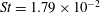 $St=1.79\times 10^{-2}$
, which corresponds to particles of approximately
$St=1.79\times 10^{-2}$
, which corresponds to particles of approximately
 $20~\unicode[STIX]{x03BC}\text{m}$
in size in the experiments of Shoshin & Dreizin (Reference Shoshin and Dreizin2002), and values of other parameters given above, show that the system tends to a stationary unidimensional state, up to the noise implicit in the simulations. The dimensionless voltage must be decreased to
$20~\unicode[STIX]{x03BC}\text{m}$
in size in the experiments of Shoshin & Dreizin (Reference Shoshin and Dreizin2002), and values of other parameters given above, show that the system tends to a stationary unidimensional state, up to the noise implicit in the simulations. The dimensionless voltage must be decreased to
 $V=2.05$
before a non-stationary structure similar to that of the previous section emerges. When it does, the plumes have less tendency than before to orderly drift, though they still collide, merge and reappear in a seemingly continuous manner.
$V=2.05$
before a non-stationary structure similar to that of the previous section emerges. When it does, the plumes have less tendency than before to orderly drift, though they still collide, merge and reappear in a seemingly continuous manner.
The stabilizing effect of the inertia of the particles at the small value of
 $St$
in the simulation is surprising at first sight. For large values of the coefficient of restitution
$St$
in the simulation is surprising at first sight. For large values of the coefficient of restitution
 $r$
, leading to rebound velocities at the lower electrode larger than
$r$
, leading to rebound velocities at the lower electrode larger than
 $q_{+}\boldsymbol{E}-\hat{\boldsymbol{\imath }}$
, the effect can be understood by noticing that the inertia decreases the number density of positive particles in the thin layer by the lower electrode where it is highest, which is where the instability developed in the absence of inertia. For small values of
$q_{+}\boldsymbol{E}-\hat{\boldsymbol{\imath }}$
, the effect can be understood by noticing that the inertia decreases the number density of positive particles in the thin layer by the lower electrode where it is highest, which is where the instability developed in the absence of inertia. For small values of
 $r$
, leading to rebound velocities smaller than
$r$
, leading to rebound velocities smaller than
 $q_{+}\boldsymbol{E}-\hat{\boldsymbol{\imath }}$
, the stabilizing effect of the particle inertia may be due to the lag it induces in the transmission of electric forces from the particles to the gas. This delays the acceleration of the gas in regions near the lower electrode where a perturbation in the density of positive particles increases the electric field, and thus hinders the mechanism of growth of the hydrodynamic instability discussed above.
$q_{+}\boldsymbol{E}-\hat{\boldsymbol{\imath }}$
, the stabilizing effect of the particle inertia may be due to the lag it induces in the transmission of electric forces from the particles to the gas. This delays the acceleration of the gas in regions near the lower electrode where a perturbation in the density of positive particles increases the electric field, and thus hinders the mechanism of growth of the hydrodynamic instability discussed above.
5 Conclusions
An analysis has been carried out of the electrodynamic fluidization of monodisperse particles of infinite electrical conductivity in a gas, assuming that the particles do not coalesce and that the effect of their inertia is negligible (small Stokes number).
Order-of-magnitude estimations show that the effect of the collisions on the dynamics of electrically charged particles is small when the characteristic number density of suspended particles is small compared to the inverse of the volume swept by a particle crossing the interelectrode gap. Stationary distributions of the particles and the electric field have been computed for given values of the applied voltage (
 $V$
) and the number of suspended particles per unit electrode area (
$V$
) and the number of suspended particles per unit electrode area (
 $N$
). Analytical results based on the work of Shoshin & Dreizin (Reference Shoshin and Dreizin2002) are given for values of
$N$
). Analytical results based on the work of Shoshin & Dreizin (Reference Shoshin and Dreizin2002) are given for values of
 $N$
small compared to the inverse of the cross-section of a particle, and numerical computations are used for larger values of
$N$
small compared to the inverse of the cross-section of a particle, and numerical computations are used for larger values of
 $N$
. These stationary distributions determine the maximum value
$N$
. These stationary distributions determine the maximum value
 $N$
can take as a function of the applied voltage. This maximum is attained in the normal operation of an electrodynamic fluidization device, when there are particles deposited at the lower electrode. It is determined by the field mechanism, whereby the electric field induced by the charge of the suspended particles, which opposes the field due to the applied voltage in the lower part of the interelectrode gap, reduces the field at the lower electrode to the minimum required for electric forces to resuspend falling particles.
$N$
can take as a function of the applied voltage. This maximum is attained in the normal operation of an electrodynamic fluidization device, when there are particles deposited at the lower electrode. It is determined by the field mechanism, whereby the electric field induced by the charge of the suspended particles, which opposes the field due to the applied voltage in the lower part of the interelectrode gap, reduces the field at the lower electrode to the minimum required for electric forces to resuspend falling particles.
Stationary solutions without collision effects become unstable when the applied voltage decreases below a certain value that depends on
 $N$
. Two instabilities may appear. One is an instability of the stationary distribution of charge associated with the large concentration of positive particles near the lower electrode. The other is a hydrodynamic instability by which an initial perturbation in the form of a localized accumulation of positive particles near the lower electrode grows and drifts away from the electrode due to the upward flow induced in the gas by the electric force on the excess of charge. This instability develops into electrohydrodynamic plumes whose dynamics is described by means of two-dimensional Lagrangian simulations. The inertia of the particles has a stabilizing effect, probably due to the delay it introduces in the response of the gas to the electric force on the particles.
$N$
. Two instabilities may appear. One is an instability of the stationary distribution of charge associated with the large concentration of positive particles near the lower electrode. The other is a hydrodynamic instability by which an initial perturbation in the form of a localized accumulation of positive particles near the lower electrode grows and drifts away from the electrode due to the upward flow induced in the gas by the electric force on the excess of charge. This instability develops into electrohydrodynamic plumes whose dynamics is described by means of two-dimensional Lagrangian simulations. The inertia of the particles has a stabilizing effect, probably due to the delay it introduces in the response of the gas to the electric force on the particles.
Acknowledgements
I am grateful to Dr Y. L. Shoshin (Eindhoven) for introducing me to this problem and for enlightening discussions, and to the anonymous referees whose comments have very much improved the paper. This work was supported by the Spanish MINECO through projects DPI2017-86547-C2-2-P and DPI2015-71901-REDT.
Appendix A. Collisions
Collisions leading to redistribution of charge require mechanical contact of the colliding particles. The relevant distance for these collisions is the particle radius
 $a$
, and the Stokes number based on this distance is larger than the small Stokes number considered in § 2 by a factor
$a$
, and the Stokes number based on this distance is larger than the small Stokes number considered in § 2 by a factor
 $L/a$
. The new Stokes number is typically large (except in the experiments of Shoshin & Dreizin (Reference Shoshin and Dreizin2002) with
$L/a$
. The new Stokes number is typically large (except in the experiments of Shoshin & Dreizin (Reference Shoshin and Dreizin2002) with
 $10~\unicode[STIX]{x03BC}\text{m}$
aluminium particles, which are unusually small and light). Thus the effect of the inertia of the particles is large compared to the hydrodynamic drag during collisions, while the opposite is true between collisions.
$10~\unicode[STIX]{x03BC}\text{m}$
aluminium particles, which are unusually small and light). Thus the effect of the inertia of the particles is large compared to the hydrodynamic drag during collisions, while the opposite is true between collisions.
The effect of the electric force between colliding particles can be estimated as follows. In terms of the characteristic electric field in the gap,
 $E_{c}=V/L$
, the typical charge of the particles is
$E_{c}=V/L$
, the typical charge of the particles is
 $q_{c}=\unicode[STIX]{x1D6FC}\unicode[STIX]{x1D716}_{0}a^{2}E_{c}$
and their typical velocity is
$q_{c}=\unicode[STIX]{x1D6FC}\unicode[STIX]{x1D716}_{0}a^{2}E_{c}$
and their typical velocity is
 $v_{c}=q_{c}E_{c}/c_{f}$
. The electrostatic energy of two charged particles whose centres are separated a distance
$v_{c}=q_{c}E_{c}/c_{f}$
. The electrostatic energy of two charged particles whose centres are separated a distance
 $2a$
is
$2a$
is
 $q_{c}^{2}/(8\unicode[STIX]{x03C0}\unicode[STIX]{x1D716}_{0}a)$
, and the ratio of this energy to the kinetic energy of the particles (
$q_{c}^{2}/(8\unicode[STIX]{x03C0}\unicode[STIX]{x1D716}_{0}a)$
, and the ratio of this energy to the kinetic energy of the particles (
 $mv_{c}^{2}$
) is
$mv_{c}^{2}$
) is
 $$\begin{eqnarray}S=\frac{c_{f}^{2}L^{2}}{8\unicode[STIX]{x03C0}m\unicode[STIX]{x1D716}_{0}aV^{2}}.\end{eqnarray}$$
This ratio is small, in the range
 $3.2\times 10^{-3}$
–
$3.2\times 10^{-3}$
–
 $8\times 10^{-3}$
in the experiments of Shoshin and Dreizin, which justifies neglecting electric forces in particle collisions.
$8\times 10^{-3}$
in the experiments of Shoshin and Dreizin, which justifies neglecting electric forces in particle collisions.
Electric forces may be important in other interactions, with impact parameter larger than
 $2a$
. These, however, do not involve mechanical contact or redistribution of charge between the particles, while the exchanges of momentum and energy are irrelevant when the effect of the particle inertia is negligible between collisions.
$2a$
. These, however, do not involve mechanical contact or redistribution of charge between the particles, while the exchanges of momentum and energy are irrelevant when the effect of the particle inertia is negligible between collisions.

Figure 9. Sketch of the excess and defect of charge induced by an external electric field on colliding particles.
Collisions occur in the presence of an external electric field additional to the field induced by the charges of the colliding particles. In the absence of an external field, the charges
 $q_{1}$
and
$q_{1}$
and
 $q_{2}$
of the particles, assumed to be perfect conductors, would be equally distributed between then, each emerging with a charge
$q_{2}$
of the particles, assumed to be perfect conductors, would be equally distributed between then, each emerging with a charge
 $(q_{1}+q_{2})/2$
. However, the external field leads to an additional redistribution of the charge which can be computed as follows. Since the effect of the inertia is negligible between collisions, the velocities of the particles relative to the gas align with the external field, and collisions occur when the more charged particle overtakes the less charged particle or the two particles approach head on. Consider first the special case sketched in figure 9(a), in which the line joining the centres of the particles is parallel to the external field. The electrostatic problem can be solved by inversion about the point of contact, which transforms the problem to that of a dipole between two parallel planes, followed by the method of images (Maxwell Reference Maxwell1881). The excess of charge induced by the external field in the upper sphere of figure 9(a), equal to the defect of charge induced in the lower sphere, is
$(q_{1}+q_{2})/2$
. However, the external field leads to an additional redistribution of the charge which can be computed as follows. Since the effect of the inertia is negligible between collisions, the velocities of the particles relative to the gas align with the external field, and collisions occur when the more charged particle overtakes the less charged particle or the two particles approach head on. Consider first the special case sketched in figure 9(a), in which the line joining the centres of the particles is parallel to the external field. The electrostatic problem can be solved by inversion about the point of contact, which transforms the problem to that of a dipole between two parallel planes, followed by the method of images (Maxwell Reference Maxwell1881). The excess of charge induced by the external field in the upper sphere of figure 9(a), equal to the defect of charge induced in the lower sphere, is
 $q_{E0}=\unicode[STIX]{x1D6FE}_{0}\unicode[STIX]{x1D716}_{0}a^{2}E$
with
$q_{E0}=\unicode[STIX]{x1D6FE}_{0}\unicode[STIX]{x1D716}_{0}a^{2}E$
with
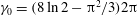 $\unicode[STIX]{x1D6FE}_{0}=(8\ln 2-\unicode[STIX]{x03C0}^{2}/3)2\unicode[STIX]{x03C0}$
. In the more general case of figure 9(b), only the component of the external field parallel to the line joining the centres contributes to the redistribution of charge between the spheres, and the excess and defect of charge are
$\unicode[STIX]{x1D6FE}_{0}=(8\ln 2-\unicode[STIX]{x03C0}^{2}/3)2\unicode[STIX]{x03C0}$
. In the more general case of figure 9(b), only the component of the external field parallel to the line joining the centres contributes to the redistribution of charge between the spheres, and the excess and defect of charge are
 $$\begin{eqnarray}q_{E}=\unicode[STIX]{x1D6FE}_{0}\unicode[STIX]{x1D716}_{0}a^{2}E\sqrt{1-\left(\frac{e}{2a}\right)^{2}},\end{eqnarray}$$
where
 $e$
is the impact parameter of the collision. If all the values of
$e$
is the impact parameter of the collision. If all the values of
 $e$
between 0 and
$e$
between 0 and
 $2a$
are equiprobable, the mean value of the excess and defect of charge is
$2a$
are equiprobable, the mean value of the excess and defect of charge is
 $$\begin{eqnarray}\bar{q}_{E}=\frac{1}{4\unicode[STIX]{x03C0}a^{2}}\int _{0}^{2a}q_{E}2\unicode[STIX]{x03C0}e\,\text{d}e=\unicode[STIX]{x1D6FE}\unicode[STIX]{x1D716}_{0}a^{2}E\quad \text{with }\unicode[STIX]{x1D6FE}=\frac{2}{3}\unicode[STIX]{x1D6FE}_{0}\approx 9.45.\end{eqnarray}$$
For completeness, collisions with negligible inertial effects, which could be relevant for suspensions of very small particles with
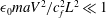 $\unicode[STIX]{x1D716}_{0}maV^{2}/c_{f}^{2}L^{2}\ll 1$
, are briefly discussed in an approximate manner. Using the estimation of
$\unicode[STIX]{x1D716}_{0}maV^{2}/c_{f}^{2}L^{2}\ll 1$
, are briefly discussed in an approximate manner. Using the estimation of
 $q_{c}$
above, the electric force between two colliding particles is of order
$q_{c}$
above, the electric force between two colliding particles is of order
 $q_{c}^{2}/(8\unicode[STIX]{x03C0}\unicode[STIX]{x1D716}_{0}a^{2})\sim q_{c}E_{c}$
, which is the order of the force due to the characteristic electric field in the gap. The mutual attraction or repulsion between colliding particles is thus important in this case and affects the value of the collision cross-section.
$q_{c}^{2}/(8\unicode[STIX]{x03C0}\unicode[STIX]{x1D716}_{0}a^{2})\sim q_{c}E_{c}$
, which is the order of the force due to the characteristic electric field in the gap. The mutual attraction or repulsion between colliding particles is thus important in this case and affects the value of the collision cross-section.

Figure 10. Sketch of particle collisions in the absence of inertia.
Consider a reference frame moving with velocity
 $(\boldsymbol{v}_{g}+m\boldsymbol{g})/c_{f}$
, where
$(\boldsymbol{v}_{g}+m\boldsymbol{g})/c_{f}$
, where
 $\boldsymbol{v}_{g}$
is the mesoscale velocity of the gas, which can be assumed to be uniform on distances of order
$\boldsymbol{v}_{g}$
is the mesoscale velocity of the gas, which can be assumed to be uniform on distances of order
 $a$
. The motion of the colliding particles takes place in a plane determined by their initial positions and the mesoscale field
$a$
. The motion of the colliding particles takes place in a plane determined by their initial positions and the mesoscale field
 $\boldsymbol{E}$
, which can also be assumed to be uniform in the collision region. Let
$\boldsymbol{E}$
, which can also be assumed to be uniform in the collision region. Let
 $\boldsymbol{x}_{1}$
and
$\boldsymbol{x}_{1}$
and
 $\boldsymbol{x}_{2}$
be the positions of the centres of the particles, and
$\boldsymbol{x}_{2}$
be the positions of the centres of the particles, and
 $q_{1}$
and
$q_{1}$
and
 $q_{2}$
their charges, with
$q_{2}$
their charges, with
 $q_{1}>q_{2}$
for definiteness. Writing
$q_{1}>q_{2}$
for definiteness. Writing
 $\boldsymbol{x}_{1}=\boldsymbol{x}_{m}+\unicode[STIX]{x1D6FF}\boldsymbol{x}$
and
$\boldsymbol{x}_{1}=\boldsymbol{x}_{m}+\unicode[STIX]{x1D6FF}\boldsymbol{x}$
and
 $\boldsymbol{x}_{2}=\boldsymbol{x}_{m}-\unicode[STIX]{x1D6FF}\boldsymbol{x}$
, the mean point
$\boldsymbol{x}_{2}=\boldsymbol{x}_{m}-\unicode[STIX]{x1D6FF}\boldsymbol{x}$
, the mean point
 $\boldsymbol{x}_{m}$
moves with velocity
$\boldsymbol{x}_{m}$
moves with velocity
 $(q_{1}-q_{2})\boldsymbol{E}/c_{f}$
. Approximating the electric force between the particles by the force between two point particles, and scaling distances with
$(q_{1}-q_{2})\boldsymbol{E}/c_{f}$
. Approximating the electric force between the particles by the force between two point particles, and scaling distances with
 $a$
and time with
$a$
and time with
 $2c_{f}a/(q_{1}-q_{2})|\boldsymbol{E}|$
,
$2c_{f}a/(q_{1}-q_{2})|\boldsymbol{E}|$
,
 $\unicode[STIX]{x1D6FF}\boldsymbol{x}=a(\unicode[STIX]{x1D6FF}x,\unicode[STIX]{x1D6FF}y)$
satisfy
$\unicode[STIX]{x1D6FF}\boldsymbol{x}=a(\unicode[STIX]{x1D6FF}x,\unicode[STIX]{x1D6FF}y)$
satisfy
 $$\begin{eqnarray}\left.\begin{array}{@{}c@{}}\displaystyle \frac{\text{d}\unicode[STIX]{x1D6FF}x}{\text{d}t}=1+\unicode[STIX]{x1D6F1}\frac{\unicode[STIX]{x1D6FF}x}{r^{3}},\quad \frac{\text{d}\unicode[STIX]{x1D6FF}y}{\text{d}t}=\unicode[STIX]{x1D6F1}\frac{\unicode[STIX]{x1D6FF}y}{r^{3}}\\ \displaystyle \text{with }r=(\unicode[STIX]{x1D6FF}x^{2}+\unicode[STIX]{x1D6FF}y^{2})^{2}\quad \text{and}\quad \unicode[STIX]{x1D6F1}=\frac{q_{1}q_{2}}{8\unicode[STIX]{x03C0}\unicode[STIX]{x1D716}_{0}|q_{1}-q_{2}||\boldsymbol{E}|a^{2}},\end{array}\right\}\end{eqnarray}$$
where the
 $x$
-axis points in the direction of
$x$
-axis points in the direction of
 $\boldsymbol{E}$
.
$\boldsymbol{E}$
.
The solution of these equations can be written in parametric form as
 $$\begin{eqnarray}\unicode[STIX]{x1D6FF}x=\frac{\unicode[STIX]{x1D6F1}}{|\unicode[STIX]{x1D6F1}|^{1/2}}\frac{\pm f(\unicode[STIX]{x1D709})-1}{\unicode[STIX]{x1D709}}\quad \text{and}\quad \unicode[STIX]{x1D6FF}y=|\unicode[STIX]{x1D6F1}|^{1/2}\frac{\sqrt{\pm 2f(\unicode[STIX]{x1D709})-2-c\unicode[STIX]{x1D709}^{2}}}{\unicode[STIX]{x1D709}}\end{eqnarray}$$
with
 $f(\unicode[STIX]{x1D709})=\sqrt{1+c\unicode[STIX]{x1D709}^{2}+\unicode[STIX]{x1D709}^{4}}$
, where
$f(\unicode[STIX]{x1D709})=\sqrt{1+c\unicode[STIX]{x1D709}^{2}+\unicode[STIX]{x1D709}^{4}}$
, where
 $\unicode[STIX]{x1D709}$
is a parameter related to time,
$\unicode[STIX]{x1D709}$
is a parameter related to time,
 $c$
is an integration constant, and the upper and lower signs in front of
$c$
is an integration constant, and the upper and lower signs in front of
 $f(\unicode[STIX]{x1D709})$
apply in different regions of the trajectory.
$f(\unicode[STIX]{x1D709})$
apply in different regions of the trajectory.
The dividing trajectory in the
 $(\unicode[STIX]{x1D6FF}x,\unicode[STIX]{x1D6FF}y)$
plane separating collisions with mechanical contact between the particles from interactions without contact is sketched in figure 10 for different ranges of
$(\unicode[STIX]{x1D6FF}x,\unicode[STIX]{x1D6FF}y)$
plane separating collisions with mechanical contact between the particles from interactions without contact is sketched in figure 10 for different ranges of
 $\unicode[STIX]{x1D6F1}$
. With reference to this figure, the problem reduces to determining
$\unicode[STIX]{x1D6F1}$
. With reference to this figure, the problem reduces to determining
 $c(\unicode[STIX]{x1D6F1})$
for the dividing trajectory, which in turn determines the limiting impact parameter
$c(\unicode[STIX]{x1D6F1})$
for the dividing trajectory, which in turn determines the limiting impact parameter
 $\unicode[STIX]{x1D6E5}(\unicode[STIX]{x1D6F1})$
in terms of which the collision cross-section is
$\unicode[STIX]{x1D6E5}(\unicode[STIX]{x1D6F1})$
in terms of which the collision cross-section is
 $4\unicode[STIX]{x03C0}\unicode[STIX]{x1D6E5}^{2}a^{2}$
. A straightforward though somewhat tedious analysis using (A 5) gives
$4\unicode[STIX]{x03C0}\unicode[STIX]{x1D6E5}^{2}a^{2}$
. A straightforward though somewhat tedious analysis using (A 5) gives
 $$\begin{eqnarray}\unicode[STIX]{x1D6E5}=\left\{\begin{array}{@{}ll@{}}\displaystyle 0 & \text{for }\unicode[STIX]{x1D6F1}>1\\ \displaystyle 1-\unicode[STIX]{x1D6F1} & \text{for }-1<\unicode[STIX]{x1D6F1}<1\\ \displaystyle 2(-\unicode[STIX]{x1D6F1})^{1/2} & \text{for }\unicode[STIX]{x1D6F1}<-1.\end{array}\right.\end{eqnarray}$$
Appendix B. Effect of a finite electrical conductivity
The assumption of infinite particle conductivity needs to be revised for non-metallic particles and for metallic particles surrounded by a layer of oxide of reduced conductivity. This is the case for aluminium particles. The electrical resistance of the oxide layer depends on its thickness and may also depend on the electric field, if quantum tunnelling is relevant (Zhebelev Reference Zhebelev1991), and on the contact pressure that appears in collisions, if electrical shorting through the layer is to be expected (Colver Reference Colver1976). In addition, surface conductivity may play a role, which brings in effects of the size, permittivity and relative humidity. In particular, the relative humidity may depend on the through flow that pushes the particles, which would thus affect the electrical properties of the particles in addition to the drag force acting on them. As kindly pointed out by a reviewer, this could partially explain the observed change of the operation characteristics of the device when a through flow is imposed. All these factors make it difficult to predict the electrical resistance of the particles. However, this resistance is known to have important effects, in particular on the maximum attainable concentration of suspended particles; see Myazdrikov (Reference Myazdrikov1984), Krivtsov & Morozov (Reference Kritsov and Morozov1985) and Bologa & Berkov (Reference Bologa and Berkov1989).
Zhebelev (Reference Zhebelev1991, Reference Zhebelev1993) modelled the effect of a finite electrical resistance on the redistribution of charge in particle–particle and particle–electrode collisions in terms of the ratio of the contact time
 $t_{c}$
to the electric relaxation time
$t_{c}$
to the electric relaxation time
 $t_{e}$
. For an elastic collision of a spherical particle and a planar electrode of the same material, the first of these times is (Landau & Lifshitz Reference Landau and Lifshitz1986)
$t_{e}$
. For an elastic collision of a spherical particle and a planar electrode of the same material, the first of these times is (Landau & Lifshitz Reference Landau and Lifshitz1986)
 $$\begin{eqnarray}t_{c}=3.78\frac{(1-\unicode[STIX]{x1D707}_{s}^{2})^{2/5}m^{2/5}}{E_{s}^{2/5}a^{1/5}v^{1/5}},\end{eqnarray}$$
where
 $E_{s}$
and
$E_{s}$
and
 $\unicode[STIX]{x1D707}_{s}$
are the elastic modulus and the Poisson modulus of the material,
$\unicode[STIX]{x1D707}_{s}$
are the elastic modulus and the Poisson modulus of the material,
 $m$
and
$m$
and
 $a$
are the mass and radius of the particle, and
$a$
are the mass and radius of the particle, and
 $v$
is the velocity with which the particle impacts on the electrode. The electric relaxation time is
$v$
is the velocity with which the particle impacts on the electrode. The electric relaxation time is
 $t_{e}=\unicode[STIX]{x1D716}_{0}\unicode[STIX]{x1D716}/K$
, where
$t_{e}=\unicode[STIX]{x1D716}_{0}\unicode[STIX]{x1D716}/K$
, where
 $\unicode[STIX]{x1D716}$
and
$\unicode[STIX]{x1D716}$
and
 $K$
are effective values of the dielectric constant and the electrical conductivity of the particle. According to Zhebelev (Reference Zhebelev1991), the charge with which a particle with initial charge
$K$
are effective values of the dielectric constant and the electrical conductivity of the particle. According to Zhebelev (Reference Zhebelev1991), the charge with which a particle with initial charge
 $q$
emerges from a collision with the lower (upper) electrode is
$q$
emerges from a collision with the lower (upper) electrode is
 $q^{\prime }=q_{\pm }+(q-q_{\pm })\exp (-t_{c}/t_{e})$
, where
$q^{\prime }=q_{\pm }+(q-q_{\pm })\exp (-t_{c}/t_{e})$
, where
 $q_{\pm }$
are given by (2.12) and (2.13).
$q_{\pm }$
are given by (2.12) and (2.13).
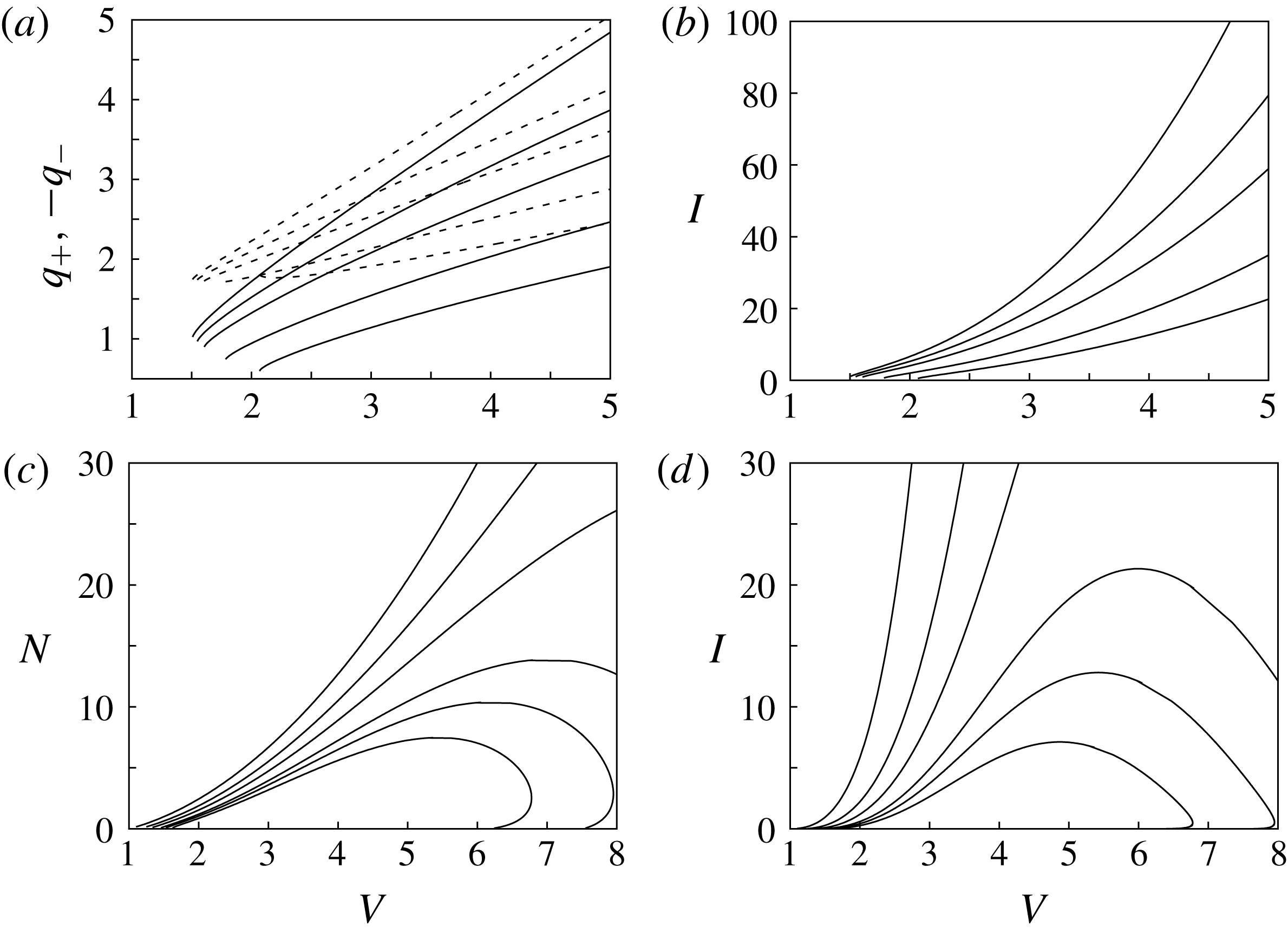
Figure 11. (a) Dimensionless charges with which the particles detach from the lower (
 $q_{+}^{\ast }$
, solid curves) and upper (
$q_{+}^{\ast }$
, solid curves) and upper (
 $q_{-}^{\ast }$
, dashed curves) electrodes, given by (B 2) as functions of the dimensionless voltage for
$q_{-}^{\ast }$
, dashed curves) electrodes, given by (B 2) as functions of the dimensionless voltage for
 $N=1$
and
$N=1$
and
 $\unicode[STIX]{x1D708}=1.5$
, 2, 3, 4 and 10, increasing from bottom to top. (b) Dimensionless electric current as a function of the dimensionless voltage for
$\unicode[STIX]{x1D708}=1.5$
, 2, 3, 4 and 10, increasing from bottom to top. (b) Dimensionless electric current as a function of the dimensionless voltage for
 $N=1$
and
$N=1$
and
 $\unicode[STIX]{x1D708}=1.5$
, 2, 3, 4 and 10, increasing from bottom to top. (c) Dimensionless number of particles per unit electrode area at the threshold of particle deposition on the lower electrode, determined by the condition
$\unicode[STIX]{x1D708}=1.5$
, 2, 3, 4 and 10, increasing from bottom to top. (c) Dimensionless number of particles per unit electrode area at the threshold of particle deposition on the lower electrode, determined by the condition
 $q_{+}^{\ast }E(0)=1$
, as a function of the dimensionless voltage for
$q_{+}^{\ast }E(0)=1$
, as a function of the dimensionless voltage for
 $\unicode[STIX]{x1D708}=1.5$
, 1.6, 1.7, 2, 2.5 and 10, increasing from bottom to top. (d) Dimensionless electric current as a function of the dimensionless voltage in the conditions of (c).
$\unicode[STIX]{x1D708}=1.5$
, 1.6, 1.7, 2, 2.5 and 10, increasing from bottom to top. (d) Dimensionless electric current as a function of the dimensionless voltage in the conditions of (c).
In this appendix, the model of Zhebelev is applied to stationary solutions in the conditions of § 3.1, when the effect of interparticle collisions is negligible. Then the charge of a particle that rebounds from the lower electrode after
 $\ell$
oscillation cycles, having collided
$\ell$
oscillation cycles, having collided
 $\ell$
times with each electrode, is
$\ell$
times with each electrode, is
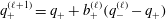 $q_{+}^{(\ell +1)}=q_{+}+b_{+}^{(\ell )}(q_{-}^{(\ell )}-q_{+})$
, where
$q_{+}^{(\ell +1)}=q_{+}+b_{+}^{(\ell )}(q_{-}^{(\ell )}-q_{+})$
, where
 $q_{-}^{(\ell )}$
is the charge with which the particle last left the upper electrode and
$q_{-}^{(\ell )}$
is the charge with which the particle last left the upper electrode and
 $b_{+}^{(\ell )}=\exp (-t_{c+}^{(\ell )}/t_{e})$
with
$b_{+}^{(\ell )}=\exp (-t_{c+}^{(\ell )}/t_{e})$
with
 $t_{c+}^{(\ell )}$
given by (B 1) for
$t_{c+}^{(\ell )}$
given by (B 1) for
 $v=[-q_{-}^{(\ell )}E(0)+mg]/c_{f}$
. Similarly,
$v=[-q_{-}^{(\ell )}E(0)+mg]/c_{f}$
. Similarly,
 $q_{-}^{(\ell +1)}=q_{-}+b_{-}^{(\ell )}(q_{+}^{(\ell )}-q_{-})$
with
$q_{-}^{(\ell +1)}=q_{-}+b_{-}^{(\ell )}(q_{+}^{(\ell )}-q_{-})$
with
 $b_{-}^{(\ell )}=\exp (-t_{c-}^{(\ell )}/t_{e})$
and
$b_{-}^{(\ell )}=\exp (-t_{c-}^{(\ell )}/t_{e})$
and
 $t_{c-}^{(\ell )}$
given by (B 1) for
$t_{c-}^{(\ell )}$
given by (B 1) for
 $v=[q_{+}^{(\ell )}E(L)-mg]/c_{f}$
. After a large number of oscillation cycles, in the limit
$v=[q_{+}^{(\ell )}E(L)-mg]/c_{f}$
. After a large number of oscillation cycles, in the limit
 $\ell \rightarrow \infty$
, the charges of the particles bouncing off the lower and upper electrodes settle to the values
$\ell \rightarrow \infty$
, the charges of the particles bouncing off the lower and upper electrodes settle to the values
 $$\begin{eqnarray}q_{+}^{\ast }=\frac{1-b_{+}^{\ast }}{1-b_{+}^{\ast }b_{-}^{\ast }}q_{+}+\frac{b_{+}^{\ast }(1-b_{-}^{\ast })}{1-b_{+}^{\ast }b_{-}^{\ast }}q_{-}\quad \text{and}\quad q_{-}^{\ast }=\frac{b_{-}^{\ast }(1-b_{+}^{\ast })}{1-b_{+}^{\ast }b_{-}^{\ast }}q_{+}+\frac{1-b_{-}^{\ast }}{1-b_{+}^{\ast }b_{-}^{\ast }}q_{-},\end{eqnarray}$$
where dimensionless variables are used,
 $q_{+}=E(0)$
,
$q_{+}=E(0)$
,
 $q_{-}=-E(1)$
, and
$q_{-}=-E(1)$
, and
 $$\begin{eqnarray}\left.\begin{array}{@{}c@{}}\displaystyle b_{+}^{\ast }=\exp \left\{-\frac{\unicode[STIX]{x1D708}}{[1-q_{-}^{\ast }E(0)]^{1/5}}\right\}\quad \text{and}\quad b_{-}^{\ast }=\exp \left\{-\frac{\unicode[STIX]{x1D708}}{[q_{+}^{\ast }E(1)-1]^{1/5}}\right\}\\ \displaystyle \text{with }\unicode[STIX]{x1D708}=\frac{t_{c0}}{t_{e}},\quad t_{c0}=3.78\frac{(1-\unicode[STIX]{x1D707}_{s}^{2})^{2/5}c_{f}^{1/5}m^{1/5}}{E_{s}^{2/5}a^{1/5}g^{1/5}}.\end{array}\right\}\end{eqnarray}$$
The analysis of § 3.1 can be redone with these modified charges of the particles. Figure 11(a,b) show the values of the charges and the electric current as functions of the voltage for
 $N=1$
and various values of
$N=1$
and various values of
 $\unicode[STIX]{x1D708}$
. As could have been expected, the charges and the current decrease when the effective conductivity, thus
$\unicode[STIX]{x1D708}$
. As could have been expected, the charges and the current decrease when the effective conductivity, thus
 $\unicode[STIX]{x1D708}$
, decreases. Figure 11(c,d) show the dimensionless number of suspended particles
$\unicode[STIX]{x1D708}$
, decreases. Figure 11(c,d) show the dimensionless number of suspended particles
 $N$
and the electric current
$N$
and the electric current
 $I$
as functions of the voltage at the threshold of particle deposition, determined by the condition
$I$
as functions of the voltage at the threshold of particle deposition, determined by the condition
 $q_{+}^{\ast }E(0)=1$
, for various values of
$q_{+}^{\ast }E(0)=1$
, for various values of
 $\unicode[STIX]{x1D708}$
. For a given voltage,
$\unicode[STIX]{x1D708}$
. For a given voltage,
 $N$
and
$N$
and
 $I$
decrease with
$I$
decrease with
 $\unicode[STIX]{x1D708}$
. For any
$\unicode[STIX]{x1D708}$
. For any
 $\unicode[STIX]{x1D708}<\infty$
, both magnitudes attain maximum values for a certain voltage and decrease when the voltage is further increased.
$\unicode[STIX]{x1D708}<\infty$
, both magnitudes attain maximum values for a certain voltage and decrease when the voltage is further increased.
The cause of this non-monotonic behaviour can be described as follows. The electric field at the upper electrode and the value of the negative charge of the particles that detach from it (
 $-q_{-}^{\ast }$
) increase with the applied voltage. The velocity with which these particles hit the lower electrode also increases. This, however, decreases the contact time of the particles with the lower electrode (see (B 1)), and the positive charge with which the particles rebound. The electric field at the lower electrode must increase in order to satisfy the condition
$-q_{-}^{\ast }$
) increase with the applied voltage. The velocity with which these particles hit the lower electrode also increases. This, however, decreases the contact time of the particles with the lower electrode (see (B 1)), and the positive charge with which the particles rebound. The electric field at the lower electrode must increase in order to satisfy the condition
 $q_{+}^{\ast }E(0)=1$
, and this limits the maximum amount of space charge (thus
$q_{+}^{\ast }E(0)=1$
, and this limits the maximum amount of space charge (thus
 $N$
), which tends to reduce this field, to a value that first increases and then decreases with increasing
$N$
), which tends to reduce this field, to a value that first increases and then decreases with increasing
 $V$
. The velocity of the positive particles tends to zero at any point in the gap when
$V$
. The velocity of the positive particles tends to zero at any point in the gap when
 $N\rightarrow 0$
on the rightmost branch of the curves.
$N\rightarrow 0$
on the rightmost branch of the curves.


