2.1 Numerical method

In this study, we perform numerical simulations using an in-house hybrid unstructured CFD code which solves the unsteady Reynolds-averaged Navier–Stokes (URANS) equations using a cell-centred finite volume approach. The integral form of the two-dimensional compressible URANS equations with the S–A turbulence model (Spalart & Allmaras Reference Spalart and Allmaras1992) can be written for a cell of volume $\unicode[STIX]{x1D6FA}$ limited by a surface $\unicode[STIX]{x1D6F4}$ and with an outer normal vector $\boldsymbol{n}$ . The equation can be expressed as

(2.1) $$\begin{eqnarray}\displaystyle \frac{\unicode[STIX]{x2202}}{\unicode[STIX]{x2202}t}\int _{\unicode[STIX]{x1D6FA}}\boldsymbol{W}\,\text{d}\unicode[STIX]{x1D6FA}+\oint _{\unicode[STIX]{x1D6F4}}\boldsymbol{E}(\boldsymbol{W},\boldsymbol{V}_{grid})\boldsymbol{\cdot }\boldsymbol{n}\,\text{d}\unicode[STIX]{x1D6F4}-\oint _{\unicode[STIX]{x1D6F4}}\boldsymbol{F}(\boldsymbol{W})\boldsymbol{\cdot }\boldsymbol{n}\,\text{d}\unicode[STIX]{x1D6F4}=\int _{\unicode[STIX]{x1D6FA}}\boldsymbol{H}\,\text{d}\unicode[STIX]{x1D6FA}, & & \displaystyle\end{eqnarray}$$

where $\boldsymbol{W}$ is a five-component vector of the conservative variables $\boldsymbol{W}=[\unicode[STIX]{x1D70C}\;\;\unicode[STIX]{x1D70C}u\;\;\unicode[STIX]{x1D70C}v\unicode[STIX]{x1D70C}E\;\;\unicode[STIX]{x1D70C}\tilde{\unicode[STIX]{x1D708}}]^{\text{T}}$ ; $\unicode[STIX]{x1D70C}$ is the density; $u,v$ are respectively the $x$ -wise and $y$ -wise components of the velocity vector of the flow; $E$ denotes the specific total energy; and $\tilde{\unicode[STIX]{x1D708}}$ denotes the working variable of the S–A turbulence model. Here, $\boldsymbol{E}$ , $\boldsymbol{F}$ and $\boldsymbol{H}$ are the inviscid flux, viscous flux and source term respectively.

The spatial discretization and time integration of the turbulence model equation and the mean flow equations are carried out in a loosely coupled way. The second-order advection upstream splitting method (AUSM) scheme is used to evaluate the inviscid flux with a reconstruction technique (Liu et al. Reference Liu, Zhang, Jiang and Ye2016b ). The viscous flux term is discretized by the standard central scheme. In the turbulence model, the convective term is discretized by the second-order AUSM scheme and the destruction term by the second-order central scheme. For unsteady computations, the dual time stepping method is used to solve the governing equations. At the sub-iteration, the fourth-stage Runge–Kutta scheme is used with a local time stepping and residual smoothing for acceleration of convergence. A no-slip wall boundary condition is applied to the airfoil surface. Moreover, the far-field boundary is assigned with a non-reflective boundary condition.

A moving boundary is involved in the control simulations due to the motion of the trailing-edge flap. Thus, a grid deformation method must be used to match the grid with the new airfoil position. The grid deformation scheme is based on the radial basis function (RBF) interpolation method (Wang, Mian & Ye Reference Wang, Mian and Ye2015). A compact Wendland C2 function is chosen as the basis function.

2.2 Validation of the buffet flow

The transonic buffet flow over a NACA 0012 airfoil is used as a test case in this study. The actuator is a 15 %-chord-length flap from the trailing edge, and its axis is located at 85 % of the chord (figure 1). Here, $\unicode[STIX]{x1D6FC}$ is the free-stream angle of attack and $\unicode[STIX]{x1D6FD}$ is the flap rotation angle. The computational domain around the airfoil is discretized by a hybrid unstructured grid. The far field extends approximately 20 chords away from the airfoil. There are 25 361 surface nodes and 40 layers of structured viscous grids around the airfoil. The distance between the first layer and the wall in the perpendicular direction is $5\times 10^{-6}$ chords ( $y^{+}\sim 1$ ). The physical time step adopted is $2.94\times 10^{-4}$  s (the non-dimensional one is 0.1).

Figure 1. Flow and actuator set-up for the simulations. The actuator is a 15 %-chord-length flap from the trailing edge. Here, $\unicode[STIX]{x1D6FD}$ is the flap rotation angle. It is determined by the control laws in the control process, while it is zero without control.

We first calculate the transonic buffet flow on a stationary NACA 0012 airfoil (without control). Figure 2 shows the comparison of the buffet onset boundary, in which the circles represent the data from the experiment conducted by Doerffer et al. (Reference Doerffer, Hirsch and Dussauge2011) and the solid line represents the computational results from the present URANS method. As can be seen, the experimental data and URANS calculations are in good agreement. At a Mach number of $M=0.70$ , the calculated buffet onset angle is $4.80^{\circ }$ , which is very close to the $4.74^{\circ }$ obtained from experiment. For other validations, including convergence studies on the grid and time step, one can refer to Gao et al. (Reference Gao, Zhang, Liu, Ye and Jiang2015) and Zhang et al. (Reference Zhang, Gao, Liu, Ye and Jiang2015a ). The strongest buffet loads occur at $5.5^{\circ }$ with a Mach number of 0.70. Therefore, we choose the case of $M=0.70$ , $\unicode[STIX]{x1D6FC}=5.5^{\circ }$ and Reynolds number $Re=3\times 10^{6}$ to perform open-loop and closed-loop control. Figure 3 shows the time histories of the lift and pitching moment coefficients at $M=0.70$ , $\unicode[STIX]{x1D6FC}=5.5^{\circ }$ and $Re=3\times 10^{6}$ initiated from the unstable steady flow. Figure 4 shows the power spectrum densities (PSDs) of the lift coefficient and the pitching moment coefficient. It can be seen that the buffet frequency is 0.2 in the non-dimensional reduced frequency scale. The reduced buffet frequency is defined as $k_{b}=\unicode[STIX]{x03C0}f_{b}c/U_{\infty }$ , where $f_{b}$ is the buffet frequency, $c$ is the chord length of the airfoil and $U_{\infty }$ denotes the velocity of the free stream.

Figure 2. Comparison of the buffet onset boundary between the present calculation and experiment.

Figure 3. Time histories of (a) lift and (b) pitching moment coefficients at $M=0.70$ , $\unicode[STIX]{x1D6FC}=5.5^{\circ }$ and $Re=3\times 10^{6}$ .

Figure 4. Power spectrum density analyses of aerodynamic responses at $M=0.70$ , $\unicode[STIX]{x1D6FC}=5.5^{\circ }$ and $Re=3\times 10^{6}$ for (a) the lift coefficient and (b) the pitching moment coefficient.

Because the transonic buffet flow exhibits periodic features, a DMD technique with an improved criterion (Kou & Zhang Reference Kou and Zhang2017a ) is used to extract the dominant frequency information and coherent flow structures of the buffet flow. As shown in figure 3(a), 300 snapshots from $t=621$ to $t=827$ in the limit cycle state are recorded as the sampling dataset for the DMD analysis. From previous studies (Schmid Reference Schmid2010; Kou & Zhang Reference Kou and Zhang2017a ), it is sufficiently accurate to illustrate the dynamics of an unstable periodic flow using no more than 10 dominant modes. Therefore, we select the first four dominant modes (all are conjugate modes except for the first one; thus, in total, seven modes are selected) in the present study. All Ritz eigenvalues and the seven selected dominant eigenvalues are shown in figure 5. The dashed line represents the unit circle. We notice that the eigenvalues are located in the vicinity of this circle, which is consistent with the snapshots taken from the fully developed limit cycle state. The first four dominant global modes characterized by the pressure contours are shown in figure 6, and the corresponding reduced frequencies and growth rates are shown in table 1. We notice that both the growth rate and the frequency are zero for the first mode. It is a static mode, close to the mean flow field. All of the other modes reflect the oscillating features resulting from shock waves. From table 1, the growth rates of these modes are also nearly zero because the snapshots are recorded from the limit cycle state. We also note that the reduced frequency of mode 2 is 0.196, which is equal to the buffet frequency from CFD simulation. The other mode frequencies are two or three times the buffet frequency. Therefore, mode 2 is the most important coherent global mode for the present buffet flow, which should be focused on to address the most relevant changes in the flow field and physical mechanisms under the control action.

Figure 5. The Ritz eigenvalues of the four dominant global modes among all modes by the DMD technique.

Table 1. Growth rates and reduced frequencies of the dominant DMD modes.

Figure 6. The first four dominant global modes from the DMD technique for a transonic buffet flow in the limit cycle state: (a) mode 1, (b) mode 2, (c) mode 3 and (d) mode 4.

3.1 Unstable steady base flow

The transonic buffet flow under consideration is unstable, which makes it challenging to construct a linear model for two reasons. First, the growing amplitudes of the aerodynamic forces or shock oscillations will ultimately give rise to a limit cycle behaviour (figure 3), which is certainly not linear. Second, the forced response under the limit cycle system is unbounded, meaning that some standard techniques to form a linear model cannot be used. Therefore, the first step, training, must be constructed with appropriate forcing signals based on the unstable steady solution. That is, the starting point to construct a linear ROM is to obtain the unstable steady base flow. The unstable steady base flow is a term often used in stability studies dealing with laminar flows, and here we employ it to denote the steady solution of the transonic buffet.

In contrast to the time-averaged flow, the steady base flow strictly satisfies the governing equations and boundary conditions in the mathematical form. It plays an important role in the modelling of unsteady flow and stability analysis (Dowell & Hall Reference Dowell and Hall2001; Illingworth et al. Reference Illingworth, Morgans and Rowley2012). Researchers have proposed many methods to obtain the steady base flow, like the Newton–Raphson technique (Barbagallo, Sipp & Schmid Reference Barbagallo, Sipp and Schmid2009, Reference Barbagallo, Sipp and Schmid2011; Weller et al. Reference Weller, Camarri and Iollo2009), selective frequency damping (Åkervik et al. Reference Åkervik, Brandt, Henningson, Hoepffner, Marxen and Schlatter2006; Jordi, Cotter & Sherwin Reference Jordi, Cotter and Sherwin2014; Flinois & Morgans Reference Flinois and Morgans2016) and control (Illingworth et al. Reference Illingworth, Morgans and Rowley2012). In our recent work (Gao et al. Reference Gao, Zhang and Ye2016b ), the unstable steady solution of buffet flow is obtained by a feedback control. Under the assumed control law, the unsteadiness of the buffet flow is stabilized without any changes in the initial flow condition, such as the angle of attack, airfoil shape, and so on. The stabilized flow is the steady base flow for the given buffet state, which is used as the initial flow condition in the training process.

Figure 8 shows the pressure contours and streamlines of the steady base flow field at $M=0.70$ , $\unicode[STIX]{x1D6FC}=5.5^{\circ }$ and $Re=3\times 10^{6}$ . It can be seen that the shock wave remains at 20 % chord behind the leading edge of the airfoil, resulting in a complete separation from $0.22c$ . The comparison of the pressure coefficient between the steady base flow and the time-averaged flow is shown in figure 9. There is a prominent difference around the shock wave, which consequently leads to the aerodynamic force, lift and pitching moment coefficients of the steady base flow being slightly larger than those of the time-averaged flow. Figure 10 presents the evolution of the aerodynamic forces ( $t<850$ in figure 3), which are plotted in the logarithm scale. When the non-dimensional time $t$ is less than 400, the amplitude of the aerodynamic coefficients is smaller than 0.015. At this stage, the evolution develops by exponential growth, which we define as the linear stage. For $t>400$ , the growing amplitude of the unstable aerodynamics ultimately reaches a nonlinear limit cycle oscillation. Therefore, the training process must finish during the linear stage.

Figure 8. Pressure contours and streamlines of the unstable steady base flow at $M=0.70$ , $\unicode[STIX]{x1D6FC}=5.5^{\circ }$ and $Re=3\times 10^{6}$ .

Figure 9. Comparison of the pressure coefficient between the time-averaged flow and the steady base flow.

Figure 10. Evolution of (a) the lift and (b) the pitching moment coefficients based on the steady base flow plotted in logarithm scale.

As shown in figure 11(a), a chirp signal with an increasing frequency is designed as the input to establish the ROM. Figure 11(b) shows the PSD analysis of the signal. Its dominant reduced frequency is varied from 0.1 to 0.5, covering the buffet frequency. Then, the training is conducted by CFD simulations at $M=0.70$ , $\unicode[STIX]{x1D6FC}=5.5^{\circ }$ based on the steady base flow, in which the flap oscillation follows the input training signal, and the outputs (lift coefficient $C_{l}$ and pitching moment coefficient $C_{m}$ ) are recorded. The non-dimensional time step is 0.1.

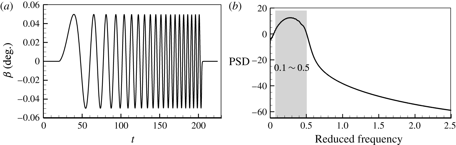
Figure 11. (a) Time history and (b) PSD analysis of the training signal.

In the training process, the flow fields are also recorded as snapshots. They are then analysed by the DMD technique. The first four dominant global modes with pressure contours are shown in figure 12, and the corresponding growth rates and reduced frequencies are shown in table 2. Similarly to the DMD modes of the fully developed buffet flow (refer to figure 6), the first mode of the present training flow is also a static mode with zero growth rate and zero frequency. This mode is very close to the steady base flow because the training is, in essence, a set of small disturbances to the base flow. From table 2, we can see that the frequency of mode 3 is zero, but its growth rate is a positive value, which means that this is a shift mode. The range of shock motions will be amplified during the training process. We also notice that modes 2 and 4 share similar flow structures and frequencies which are close to the buffet frequency. Both are correlative modes towards the dominant buffet mode (mode 2 in figure 6) under the influence of training disturbances. Modes 2 and 4 have positive growth rates, which corresponds to the divergent response of the output in figure 13. We also investigate modes 2 and 4 (dominant global mode) with respect to the conservative variables $\unicode[STIX]{x1D70C}$ and $\unicode[STIX]{x1D70C}u$ , and compare them with the coherent structure of the dominant global mode around a supercritical airfoil studied by Sartor et al. (Reference Sartor, Mettot and Sipp2015a ). We find that the coherent flow structures are similar between them. These modes are most energetic within the shock wave. However, some details, such as the position and intensity of the shock wave, are different, which is caused by differences in the buffet conditions and airfoil shapes.

Figure 12. The first four dominant global modes from the DMD technique for the training process: (a) mode 1, (b) mode 2, (c) mode 3 and (d) mode 4.

Table 2. Growth rates and reduced frequencies of the dominant DMD modes.

3.2 Linear model by the identification method

System identification is a well-established technique for the recovery of deterministic and/or stochastic dynamical systems from their output to input signals. In the present study, we are interested in modelling the unstable transonic buffet flow by processing measured data sequences for $\boldsymbol{u}$ and $\boldsymbol{y}$ based on the ARX method.

Figure 13. Identified aerodynamic coefficients of (a) the lift moment and (b) the pitching moment compared with those of CFD simulations.

Given that unsteady loads are computed in the discrete-time domain, the unified form can be expressed as follows:

(3.1) $$\begin{eqnarray}\displaystyle \boldsymbol{y}(k)=\mathop{\sum }_{i=1}^{na}\unicode[STIX]{x1D63C}_{i}\boldsymbol{y}(k-i)+\mathop{\sum }_{i=0}^{nb-1}\unicode[STIX]{x1D63D}_{i}\boldsymbol{u}(k-i), & & \displaystyle\end{eqnarray}$$

where $\boldsymbol{y}$ is the system output vector and $\boldsymbol{u}$ is the system input. Here, $\unicode[STIX]{x1D63C}_{i}$ and $\unicode[STIX]{x1D63D}_{i}$ are the constant coefficients to be estimated. The orders of the model chosen in this study are $na$ and $nb$ . The least-squares method is used to estimate unknown model parameters. To ensure that the mean is zero, constant levels are removed from the initial data before they are estimated.

In order to complete the state-space aerodynamic analysis, we define a state $\hat{\boldsymbol{x}}(k)$ consisting of ( $na+nb-1$ ) states as follows:

(3.2) $$\begin{eqnarray}\displaystyle \hat{\boldsymbol{x}}(k)=[\boldsymbol{y}(k-1),\ldots ,\boldsymbol{y}(k-na),\boldsymbol{u}(k-1),\ldots ,\boldsymbol{u}(k-nb+1)]^{\text{T}}. & & \displaystyle\end{eqnarray}$$

The state-space form of the discrete-time aerodynamic model is

(3.3) $$\begin{eqnarray}\displaystyle \left.\begin{array}{@{}l@{}}\hat{\boldsymbol{x}}(k+1)=\tilde{\unicode[STIX]{x1D63C}}\boldsymbol{x}(k)+\tilde{\unicode[STIX]{x1D63D}}\boldsymbol{u}(k),\\ \boldsymbol{y}(k)=\tilde{\unicode[STIX]{x1D63E}}\boldsymbol{x}(k)+\tilde{\unicode[STIX]{x1D63F}}\boldsymbol{u}(k),\end{array}\right\} & & \displaystyle\end{eqnarray}$$

where

(3.4) $$\begin{eqnarray}\displaystyle & \displaystyle \tilde{\unicode[STIX]{x1D63C}}=\left[\begin{array}{@{}cccccccccc@{}}A_{1} & A_{2} & \cdots \, & A_{na-1} & A_{na} & B_{1} & B_{2} & \cdots \, & B_{nb-2} & B_{nb-1}\\ 1 & 0 & \cdots \, & 0 & 0 & 0 & 0 & \cdots \, & 0 & 0\\ \vdots & 1 & \cdots \, & 0 & 0 & 0 & 0 & \cdots \, & 0 & 0\\ \vdots & \vdots & \ddots & \vdots & \vdots & \vdots & \vdots & \ddots & \vdots & \vdots \\ 0 & 0 & \cdots \, & 1 & 0 & 0 & 0 & \cdots \, & 0 & 0\\ 0 & 0 & \cdots \, & 0 & 0 & 0 & 0 & \cdots \, & 0 & 0\\ 0 & 0 & \cdots \, & 0 & 0 & 1 & 0 & \cdots \, & 0 & 0\\ 0 & 0 & \cdots \, & 0 & 0 & 0 & 1 & \cdots \, & 0 & 0\\ \vdots & \vdots & \ddots & \vdots & \vdots & \vdots & \vdots & \ddots & \vdots & \vdots \\ 0 & 0 & \cdots \, & 0 & 0 & 0 & 0 & \cdots \, & 1 & 0\\ \end{array}\right], & \displaystyle\end{eqnarray}$$

(3.5) $$\begin{eqnarray}\displaystyle & \displaystyle \tilde{\unicode[STIX]{x1D63D}}=\left[\begin{array}{@{}cccccccccc@{}}B_{0} & 0 & 0 & \cdots \, & 0 & 1 & 0 & 0 & \cdots \, & 0\\ \end{array}\right]^{\text{T}}, & \displaystyle\end{eqnarray}$$

(3.6) $$\begin{eqnarray}\displaystyle & \displaystyle \tilde{\unicode[STIX]{x1D63E}}=\left[\begin{array}{@{}cccccccccc@{}}A_{1} & A_{2} & \cdots \, & A_{na-1} & A_{na} & B_{1} & B_{2} & \cdots \, & B_{nb-2} & B_{nb-1}\end{array}\right], & \displaystyle\end{eqnarray}$$

(3.7) $$\begin{eqnarray}\displaystyle & \displaystyle \tilde{\unicode[STIX]{x1D63F}}=[B_{0}]. & \displaystyle\end{eqnarray}$$

Then, the discrete-time state-space equation is turned into the continuous-time form by bilinear transformation, and the model in the state-space form is constructed as follows:

(3.8) $$\begin{eqnarray}\displaystyle \left.\begin{array}{@{}l@{}}\dot{\hat{\boldsymbol{x}}}(t)=\hat{\unicode[STIX]{x1D63C}}\hat{\boldsymbol{x}}(t)+\hat{\unicode[STIX]{x1D63D}}\boldsymbol{u}(t),\\ \boldsymbol{y}(t)=\hat{\unicode[STIX]{x1D63E}}\hat{\boldsymbol{x}}(t)+\hat{\unicode[STIX]{x1D63F}}\boldsymbol{u}(t),\end{array}\right\} & & \displaystyle\end{eqnarray}$$

where $\hat{\boldsymbol{x}}\in \mathbb{R}^{n\ast }$ , $\boldsymbol{u}\in \mathbb{R}^{m}$ and $\boldsymbol{y}\in \mathbb{R}^{p}$ are respectively the state vector, the input vector and the output vector. We define $n^{\ast }=na+nb-1$ as the dimension of the state; $m$ and $p$ are the dimensions of the input and output respectively. Here, $\hat{\unicode[STIX]{x1D63C}}\in \mathbb{R}^{n^{\ast }\times n^{\ast }}$ , $\hat{\unicode[STIX]{x1D63D}}\in \mathbb{R}^{n^{\ast }\times m}$ and $\hat{\unicode[STIX]{x1D63E}}\in \mathbb{R}^{p\times n^{\ast }}$ are matrices calculated by the above method. This model (3.8) is referred to as ROM-ARX.

We set up the aerodynamic model at $M=0.70$ and $\unicode[STIX]{x1D6FC}=5.5^{\circ }$ to verify the method. The input and output have been recorded in the training process in § 3.1. In the present case, the output vector $\boldsymbol{y}$ contains the components of the lift coefficient $C_{l}$ and the pitching moment coefficient $C_{m}$ . The input $\boldsymbol{u}$ is the flapping angle $\unicode[STIX]{x1D6FD}$ . That is, for the present single-input double-output system, $m=1$ , $p=2$ . The comparison between CFD simulations and identified results with different orders is shown in figure 13, and identified errors are shown in table 3. The error is defined as follows:

(3.9) $$\begin{eqnarray}\displaystyle \boldsymbol{e}=\frac{\displaystyle \mathop{\sum }_{i=1}^{L}|\boldsymbol{y}(i)-\boldsymbol{y}_{iden}(i)|}{\displaystyle \mathop{\sum }_{i=1}^{L}|\boldsymbol{y}(i)|}, & & \displaystyle\end{eqnarray}$$

where $\boldsymbol{y}_{iden}$ represents the vector of identified aerodynamic forces and $L$ is the length of the training signals. It can be seen that the best identification is obtained with errors of less than 8 % when $na=nb=60$ . In this case, the established ROM-ARX ( $\hat{A},\hat{B},{\hat{C}},\hat{D}$ ) has high accuracy compared with the CFD simulation.

Once we have constructed the state-space model (3.8), the instability problem of the flow is converted into the analysis of eigenvalues of the matrix $\hat{\unicode[STIX]{x1D63C}}$ . We can obtain the unstable global fluid mode that is associated with the instability of the transonic buffet flow. The real part of the eigenvalue indicates the damping of the mode, and a positive one means that the flow is unstable. The imaginary part, in the reduced frequency scale, indicates the reduced frequency of the mode. Figure 14 displays eigenvalues of ROM-ARX with different orders at $M=0.70$ and $\unicode[STIX]{x1D6FC}=5.5^{\circ }$ . It can be seen that most eigenvalues are located in the left half of the complex plane (figure 14 a,b). There are a pair of conjugate eigenvalues lying in the right half-plane, and they are approximately convergent with the identified accuracy, as shown in figure 14(c). In addition, we notice that the imaginary parts (indicating frequency) of the eigenvalues are nearly equal to 0.2, which coincides with the buffet frequency from the CFD simulation (figure 4). This pair of eigenvalues represents the dominant unstable global mode, and its coherent flow structure is shown in mode 2 of figure 12(b). The dynamics of the buffet flow system is dominated by this pair of unstable eigenvalues.

Figure 14. Eigenvalues obtained by ROM-ARX with different orders at $M=0.70$ and $\unicode[STIX]{x1D6FC}=5.5^{\circ }$ . (b) Shows a zoomed view of the region of interest in (a) and (c) shows a zoomed view of the unstable poles in (b).

Table 3. Identified errors with different orders.

3.3 Balanced truncation model

A linear model (ROM-ARX) has been obtained in (3.8). Its dimension has been greatly reduced compared with the full-dimensional system, but it is still $O\sim (10^{2})$ in most cases, which is inconvenient for the design of the feedback control law. Moreover, it is observed that in many high-dimensional systems, the control input may only excite a few controllable modes, while the remaining modes stay stable. Therefore, we aim to find an approximate but lower-dimensional model to represent the input–output dynamics. Balanced truncation is a commonly used method, which was developed by Moore (Reference Moore1981) for stable systems. The basic idea is to discard states that have little effect on the overall model response. By finding a transformation, the controllability and observability Gramians can be transformed into equal and diagonal entries, which are called generalized Hankel singular values (HSVs). A balanced ROM can be obtained by truncating the states with small HSVs.

The standard balanced truncation method was extended to study unstable systems by Zhou, Salomon & Wu (Reference Zhou, Salomon and Wu1999), Rowley (Reference Rowley2005) and Flinois, Morgans & Schmid (Reference Flinois, Morgans and Schmid2015). It is necessary to first calculate the Gramians of the system, which represent the system input and output characteristics. For an unstable system, the controllability and observability Gramians of a continuous system (3.8) can be defined in the frequency domain as follows:

(3.10) $$\begin{eqnarray}\displaystyle \left.\begin{array}{@{}l@{}}\displaystyle \boldsymbol{M}_{c}=\frac{1}{2\unicode[STIX]{x03C0}}\int _{-\infty }^{\infty }(\text{i}\unicode[STIX]{x1D714}\unicode[STIX]{x1D644}-\hat{\unicode[STIX]{x1D63C}})^{-1}\hat{\unicode[STIX]{x1D63D}}\hat{\unicode[STIX]{x1D63D}}^{\text{T}}(-\text{i}\unicode[STIX]{x1D714}\unicode[STIX]{x1D644}-\hat{\unicode[STIX]{x1D63C}}^{\text{T}})^{-1}\,\text{d}\unicode[STIX]{x1D714},\\ \displaystyle \boldsymbol{M}_{o}=\frac{1}{2\unicode[STIX]{x03C0}}\int _{-\infty }^{\infty }(\text{i}\unicode[STIX]{x1D714}\unicode[STIX]{x1D644}-\hat{\unicode[STIX]{x1D63C}}^{\text{T}})^{-1}\hat{\unicode[STIX]{x1D63E}}\hat{\unicode[STIX]{x1D63E}}^{\text{T}}(-\text{i}\unicode[STIX]{x1D714}\unicode[STIX]{x1D644}-\hat{\unicode[STIX]{x1D63C}})^{-1}\,\text{d}\unicode[STIX]{x1D714}.\end{array}\right\} & & \displaystyle\end{eqnarray}$$

The integrals in (3.10) are bounded for unstable systems as long as the eigenvalues of $\hat{\unicode[STIX]{x1D63C}}$ are not on the imaginary axis. The full dynamics can be divided into two subspaces, one representing the unstable dynamics (the unstable global modes) and the other describing the stable dynamics required for the subsequent analysis. Since the dynamics in both subspaces are decoupled, they can be modelled separately. The system (3.8) can be transformed to

(3.11) $$\begin{eqnarray}\displaystyle \left.\begin{array}{@{}l@{}}\displaystyle \dot{\hat{\boldsymbol{x}}}=\frac{\text{d}}{\text{d}t}\left(\begin{array}{@{}c@{}}\hat{\boldsymbol{x}}_{u}\\ \hat{\boldsymbol{x}}_{s}\end{array}\right)=\left(\begin{array}{@{}cc@{}}\hat{\unicode[STIX]{x1D63C}}_{u} & \mathbf{0}\\ \mathbf{0} & \hat{\unicode[STIX]{x1D63C}}_{s}\end{array}\right)\hat{\boldsymbol{x}}+\left(\begin{array}{@{}c@{}}\hat{\unicode[STIX]{x1D63D}}_{u}\\ \hat{\unicode[STIX]{x1D63D}}_{s}\end{array}\right)\boldsymbol{u},\\ \boldsymbol{y}=\left(\begin{array}{@{}cc@{}}\hat{\unicode[STIX]{x1D63E}}_{u} & \hat{\unicode[STIX]{x1D63E}}_{s}\end{array}\right)\hat{\boldsymbol{x}}+\hat{\unicode[STIX]{x1D63F}}\boldsymbol{u},\end{array}\right\} & & \displaystyle\end{eqnarray}$$

where $\hat{\unicode[STIX]{x1D63C}}_{u}$ and $\hat{\unicode[STIX]{x1D63C}}_{s}$ are the decoupled state matrices, the eigenvalues of which are in the right and left half-complex-planes respectively, while $\hat{\boldsymbol{x}}_{u}$ and $\hat{\boldsymbol{x}}_{s}$ are the corresponding states. The dimensions of $\hat{\boldsymbol{x}}_{u}$ and $\hat{\boldsymbol{x}}_{s}$ are $n_{u}$ and $n_{s}$ respectively ( $n^{\ast }=n_{u}+n_{s}$ ). Then, we define the controllability and observability Gramians corresponding to the stable set ( $\hat{\unicode[STIX]{x1D63C}}_{s},\hat{\unicode[STIX]{x1D63D}}_{s},\hat{\unicode[STIX]{x1D63E}}_{s}$ ) describing the stable dynamics as $\boldsymbol{M}_{c}^{s}$ and $\boldsymbol{M}_{o}^{s}$ respectively. Similarly, the Gramians corresponding to the unstable set ( $\hat{\unicode[STIX]{x1D63C}}_{u},\hat{\unicode[STIX]{x1D63D}}_{u},\hat{\unicode[STIX]{x1D63E}}_{u}$ ) are defined as $\boldsymbol{M}_{c}^{u}$ and $\boldsymbol{M}_{o}^{u}$ . By introducing the transformation $\hat{\boldsymbol{x}}=\boldsymbol{T}\boldsymbol{x}$ , the Gramians of the original system can then be related to those corresponding to the subsystems through

(3.12) $$\begin{eqnarray}\displaystyle \left.\begin{array}{@{}l@{}}\boldsymbol{M}_{c}=\boldsymbol{T}\left(\begin{array}{@{}cc@{}}\boldsymbol{M}_{c}^{u} & \mathbf{0}\\ \mathbf{0} & \boldsymbol{M}_{c}^{s}\end{array}\right)\boldsymbol{T}^{\ast },\\ \boldsymbol{M}_{o}=(\boldsymbol{T}^{-1})^{\ast }\left(\begin{array}{@{}cc@{}}\boldsymbol{M}_{o}^{u} & \mathbf{0}\\ \mathbf{0} & \boldsymbol{M}_{o}^{s}\end{array}\right)\boldsymbol{T}^{-1}.\end{array}\right\} & & \displaystyle\end{eqnarray}$$

For an unstable system, we need to establish a balanced model which can (i) capture the unstable dynamics of the original system and (ii) accurately reproduce the input–output behaviour. The first requirement can be satisfied by guaranteeing that unstable modes are not truncated. All unstable global eigenvalues are used directly to represent the dynamics in the unstable subspace. This leads to an ‘exact’ model for the unstable subspace. Generally speaking, the dimension of the unstable subspace is often less than 10 for fluid systems, and so this method often requires the computation of only a few eigenvalues and eigenmodes. For the second requirement, the stable subspace is balanced by truncating the states with small HSVs (e.g. only the first $r$ states are kept). This choice has been proved to achieve an accurate description of the stable input–output behaviour with a small number of modes (Barbagallo et al. Reference Barbagallo, Sipp and Schmid2009). In this process, the input and output remain unchanged. Therefore, the primary ROM-ARX model with $n^{\ast }$ dimensions is approximated by a balanced one with $n$ dimensions ( $n=n_{u}+r$ and $n\ll n^{\ast }$ ). We refer to this balanced model as balanced ROM, which is expressed as follows:

(3.13) $$\begin{eqnarray}\displaystyle \left.\begin{array}{@{}l@{}}\dot{\boldsymbol{x}}=\unicode[STIX]{x1D63C}\boldsymbol{x}+\unicode[STIX]{x1D63D}\boldsymbol{u},\\ \boldsymbol{y}=\unicode[STIX]{x1D63E}\boldsymbol{x}+\unicode[STIX]{x1D63F}\boldsymbol{u}.\end{array}\right\} & & \displaystyle\end{eqnarray}$$

We also take the buffet flow at $M=0.7$ and $\unicode[STIX]{x1D6FC}=5.5^{\circ }$ to verify the method. In this case, there are a pair of unstable complex eigenvalues from figure 14; that is, $n_{u}=2$ . For the stable subspace, we choose $r=2$ . In this way, a balanced ROM with four dimensions is established. It is validated in the time domain by comparing the predicted results with CFD simulations under excitations of two harmonic signals. Their amplitudes are both $0.03^{\circ }$ , and their frequencies are 0.7 and 1.4 times the buffet frequency respectively. Figure 15 shows a comparison of the time histories of the lift and pitching moment coefficients between the ROMs (ROM-ARX and balanced ROM) and CFD simulations. The ROMs perform well during the initial transients, but over longer time frames they fail to capture the actual dynamics. This is not surprising as these perturbations exceed the validity range of the linear models. The dynamics of the present buffet flow is dominated by the linear characteristic, and the results obtained from the balanced ROM are in good agreement with higher-order models. The present model is the first ROM with a moving boundary for transonic buffet flow, with which it is feasible to perform model-based control law design.

Figure 15. Comparison of time responses under harmonic excitations: (a) lift coefficient and (b) pitching moment coefficient at 1.4 times the buffet frequency; (c) lift coefficient and (d) pitching moment coefficient at 0.7 times the buffet frequency.

4.1 Open-loop control

The controller proposed here is of the open-loop type; that is, the flap is driven in a prescribed periodic oscillating way. The block diagram of the open-loop control is shown in figure 16. The control law is given as

(4.1) $$\begin{eqnarray}\displaystyle \unicode[STIX]{x1D6FD}(t)=A\sin (\unicode[STIX]{x1D714}_{flap}t+\unicode[STIX]{x1D711})=A\sin (\unicode[STIX]{x1D702}\unicode[STIX]{x1D714}_{flow}t+\unicode[STIX]{x1D711}), & & \displaystyle\end{eqnarray}$$

where $A$ is the amplitude of the oscillating flap, $\unicode[STIX]{x1D714}_{flap}$ is the circular frequency of the oscillating flap, which is $\unicode[STIX]{x1D702}$ times the buffet frequency $\unicode[STIX]{x1D714}_{flow}$ , $t$ is the non-dimensional time and $\unicode[STIX]{x1D711}$ is the phase angle.

Figure 16. Block diagram of the open-loop control.

4.1.1 Effect of the flapping amplitude and frequency

We first investigate the effects of the flapping amplitude and frequency on the buffet flow. That is, the phase angle is fixed at $\unicode[STIX]{x1D711}=0$ while the amplitude $A$ and the frequency ratio $\unicode[STIX]{x1D702}$ are changed. Generally speaking, the flapping has an obvious impact on the unsteadiness of the buffet flow when the amplitude is large or the frequency ratio is close to 1 ( $\unicode[STIX]{x1D702}\sim 1$ ) (Doerffer et al. Reference Doerffer, Hirsch and Dussauge2011). A larger flapping amplitude ( $A>5^{\circ }$ ), however, often causes extra fluctuations in the aerodynamic performance. Therefore, we take two medium amplitudes, $A=2.0^{\circ }$ and $A=3.5^{\circ }$ , as examples in the present study. In order to conduct a comprehensive parameter study, the frequency ratio $\unicode[STIX]{x1D702}$ changes in a range from $\unicode[STIX]{x1D702}=0.2$ to $\unicode[STIX]{x1D702}=5.0$ , with increased resolution around $\unicode[STIX]{x1D702}\sim 1$ . It has been tested that for a wider range of ratio, the trend agrees with that of the present one.

Figure 17 shows the amplitude of the lift coefficient as a function of the frequency ratio at $A=2.0^{\circ }$ and $A=3.5^{\circ }$ . The trends of both curves are consistent. It can be seen that at most frequencies, the amplitude of the lift coefficient with the present open-loop control is larger than that of the stationary airfoil. In particular, when the flapping frequency is close to the buffet frequency ( $\unicode[STIX]{x1D702}\sim 1$ ), aerodynamic resonance occurs, resulting in an amplitude much larger than that of the stationary airfoil (Doerffer et al. Reference Doerffer, Hirsch and Dussauge2011; Iovnovich & Raveh Reference Iovnovich and Raveh2012; Sipp Reference Sipp2012). We denote the aerodynamic resonance by the term $\boldsymbol{R}$ zone. Similarly, we use $\boldsymbol{E}$ zone to represent the region of effective control. For the cases in the $\boldsymbol{E}$ zone, the amplitude of the lift coefficient is smaller than that of the stationary airfoil, for the ratio $\unicode[STIX]{x1D702}$ in the range 1.4–1.8. Figure 18 shows the oscillating frequencies of the lift coefficient with different flapping frequencies. In the case of $A=2.0^{\circ }$ (figure 18 a), the basic frequency follows the buffet frequency, while in the case of $A=3.5^{\circ }$ (figure 18 b), the basic frequency locks onto the flapping frequency and the secondary frequency equals the buffet frequency. For a smaller amplitude ( $A=2.0^{\circ }$ ), the flap oscillation only has a weak impact on the unstable buffet flow; therefore, the buffet flow is the dominant one. For a larger amplitude ( $A=3.5^{\circ }$ ), the unsteadiness caused by the oscillating flap dominates the buffet flow, transforming the basic frequency from the buffet frequency to the flapping frequency.

Figure 17. The amplitude of the lift coefficient as a function of the frequency ratio $\unicode[STIX]{x1D702}$ .

Figure 18. The relationship between the oscillating frequency of the lift coefficient and the frequency ratio $\unicode[STIX]{x1D702}$ at (a) $A=2.0^{\circ }$ and (b) $A=3.5^{\circ }$ .

4.1.2 Effect of the phase angle

The effect of the phase angle is then studied with the parameter set of $A=2.0^{\circ }$ and $\unicode[STIX]{x1D702}=1.6$ . Figure 19 shows the amplitude of the lift coefficient at different phase angles and figure 20 shows the oscillating frequency of the lift coefficient as a function of the phase angle. The phase angle step size is $30^{\circ }$ and has been reduced around $290^{\circ }$ for the increased resolution. It can be seen that the amplitude of the lift coefficient displays two dips near $90^{\circ }$ and $290^{\circ }$ , which are significantly smaller than that of the stationary airfoil without control. From figure 20, it can be seen that the oscillating frequency completely follows the flapping frequency around $290^{\circ }$ . At other phase angles, the responses of the lift coefficient display two frequencies, with the basic one equal to the buffet frequency. Therefore, the optimal phase angle is approximately $290^{\circ }$ for the present open-loop control.

Figure 19. The amplitude of the lift coefficient as a function of the phase angle.

Figure 20. The oscillating frequency of the lift coefficient at different phase angles.

Figure 21 shows the response of the lift coefficient and PSD results at $A=2^{\circ }$ , $\unicode[STIX]{x1D702}=1.6$ and $\unicode[STIX]{x1D711}=290^{\circ }$ . In this combination of control parameters, the open-loop control law can efficiently suppress buffet loads, reducing the amplitude of the lift coefficient by more than 70 % (from 0.130 to 0.035). The PSD results indicate that the oscillating frequency shifts from the buffet frequency ( $t<624$ ) to the flapping frequency ( $t>950$ ). Therefore, the present open-loop control strategy with appropriate control parameters can significantly reduce the buffet unsteadiness. However, it cannot completely suppress the unsteadiness due to the sustained disturbance of the oscillating flap on the flow. The unsteadiness at $t>950$ is caused by the prescribed flap oscillations.

Figure 21. (a) Time history of the lift coefficient and (b,c) PSD results at the stages (b) $t<624$ and (c) $t>950$ at $A=2^{\circ }$ , $\unicode[STIX]{x1D702}=1.6$ and $\unicode[STIX]{x1D711}=290^{\circ }$ . The process of this open-loop control is available as a supplementary movie at https://doi.org/10.1017/jfm.2017.344 (movie 1).

4.2 Closed-loop control by the pole assignment method

A four-dimensional balanced ROM was developed in § 3.3. The system has a pair of conjugate poles in the unstable complex plane, indicating the instability of the flow system. As the purpose of the pole assignment is to stabilize the system, it is desired to have all of the poles of the closed-loop system located in the left half of the complex plane. The block diagram of the closed-loop control is shown in figure 22, in which the feedback gain $\unicode[STIX]{x1D646}$ is solved according to the framework of the pole assignment method.

Figure 22. Closed-loop control topology.

4.2.1 Pole assignment method framework

Pole assignment is a traditional method for closed-loop control, which is essentially a special algebraic inverse eigenvalue problem (Kimura Reference Kimura1977; Franke Reference Franke2014). Its basic idea is to find a feedback gain matrix that keeps all or partial poles of the closed-loop system in the desired place.

Since the balanced truncation does not change the controllability, the balanced system in (3.13) shares the same controllability with the original system in (3.8). The Gramians defined in (3.10) are not singular matrices. Therefore, the balanced ROM ( $\unicode[STIX]{x1D63C}$ , $\unicode[STIX]{x1D63D}$ , $\unicode[STIX]{x1D63E}$ , $\unicode[STIX]{x1D63F}$ ) is controllable. According to the output feedback, the linear feedback control law is defined as a linear function of the output aerodynamics,

(4.2) $$\begin{eqnarray}\displaystyle \unicode[STIX]{x1D6FD}(t)=\boldsymbol{u}(t)=\unicode[STIX]{x1D646}\boldsymbol{y}(t), & & \displaystyle\end{eqnarray}$$

where the feedback gain is $\unicode[STIX]{x1D646}\in \mathbb{R}^{m\times p}$ . By substituting the output of (3.13) into (4.2), we can obtain

(4.3) $$\begin{eqnarray}\displaystyle \boldsymbol{u}(t)=\unicode[STIX]{x1D646}(\unicode[STIX]{x1D644}-\unicode[STIX]{x1D63F}\unicode[STIX]{x1D646})^{-1}\unicode[STIX]{x1D63E}\boldsymbol{x}(t). & & \displaystyle\end{eqnarray}$$

Then, by substituting (4.3) into the open-loop system equation (3.13), we obtain the state equation of the closed-loop system,

(4.4) $$\begin{eqnarray}\displaystyle \dot{\boldsymbol{x}}(t)=[\unicode[STIX]{x1D63C}+\unicode[STIX]{x1D63D}\unicode[STIX]{x1D646}(\unicode[STIX]{x1D644}-\unicode[STIX]{x1D63F}\unicode[STIX]{x1D646})^{-1}\unicode[STIX]{x1D63E}]\boldsymbol{x}(t). & & \displaystyle\end{eqnarray}$$

We define $\unicode[STIX]{x1D63C}_{c}=\unicode[STIX]{x1D63C}+\unicode[STIX]{x1D63D}\unicode[STIX]{x1D646}(\unicode[STIX]{x1D644}-\unicode[STIX]{x1D63F}\unicode[STIX]{x1D646})^{-1}\unicode[STIX]{x1D63E}$ , which is a function of the feedback gain $\unicode[STIX]{x1D646}$ . The characteristics of the closed-loop system are indicated by the eigenvalues (poles of the closed-loop system) of the state matrix $\unicode[STIX]{x1D63C}_{c}$ . Therefore, the poles of the closed-loop system can be modified by the feedback gain $\unicode[STIX]{x1D646}$ .

We note that the balanced ROM decouples the dynamics into stable and unstable subspaces and that the dynamics of the system is dominated by the two-dimensional unstable part of the model. Therefore, we can change the stability of the system by only assigning unstable poles; that is, a partial pole assignment technique can be used (Davison & Wang Reference Davison and Wang1975). For the static output feedback, the number of poles that can be assigned is

(4.5) $$\begin{eqnarray}\displaystyle q=\min (n,m+p-1), & & \displaystyle\end{eqnarray}$$

where $n,m$ and $p$ are the dimensions of the state, input and output respectively. The process to assign partial poles can be stated as follows.

1. (1) Define a finite self-conjugate set $\unicode[STIX]{x1D726}$ of $q$ ( $q<n$ ) complex numbers $\tilde{\unicode[STIX]{x1D706}}_{1},\tilde{\unicode[STIX]{x1D706}}_{2},\ldots ,\tilde{\unicode[STIX]{x1D706}}_{q}\in \mathbb{C}$ . For the unstable flow control, we can just assign unstable poles.

2. (2) Calculate an output feedback gain matrix $\unicode[STIX]{x1D646}$ , which can ensure that the eigenspectrum of the closed-loop system satisfies $\unicode[STIX]{x1D706}_{i}(\unicode[STIX]{x1D63C}_{c}(\unicode[STIX]{x1D646}))=\tilde{\unicode[STIX]{x1D706}}_{i},i=1,\ldots ,q$ .

The gain matrix $\unicode[STIX]{x1D646}$ is calculated by the nonlinear least-squares method. The mapping $f$ is defined by

(4.6) $$\begin{eqnarray}\displaystyle f(\unicode[STIX]{x1D646})=\left[\begin{array}{@{}c@{}}\unicode[STIX]{x1D706}_{1}(\unicode[STIX]{x1D63C}_{c}(\unicode[STIX]{x1D646}))-\tilde{\unicode[STIX]{x1D706}}_{1}\\ \cdots \\ \unicode[STIX]{x1D706}_{q}(\unicode[STIX]{x1D63C}_{c}(\unicode[STIX]{x1D646}))-\tilde{\unicode[STIX]{x1D706}}_{q}\end{array}\right]. & & \displaystyle\end{eqnarray}$$

The pole assignment is equivalent to solving the following nonlinear least-squares problem:

(4.7) $$\begin{eqnarray}\displaystyle \min _{\unicode[STIX]{x1D646}\in \mathbb{R}^{m\times p}}\hat{f}(\unicode[STIX]{x1D646}):=\frac{1}{2}\Vert f(\unicode[STIX]{x1D646})\Vert ^{2}=\frac{1}{2}\mathop{\sum }_{i=1}^{q}(\unicode[STIX]{x1D706}_{i}(\unicode[STIX]{x1D63C}_{c}(\unicode[STIX]{x1D646}))-\tilde{\unicode[STIX]{x1D706}}_{i})^{\ast }(\unicode[STIX]{x1D706}_{i}(\unicode[STIX]{x1D63C}_{c}(\unicode[STIX]{x1D646}))-\tilde{\unicode[STIX]{x1D706}}_{i}), & & \displaystyle\end{eqnarray}$$

where $f(\unicode[STIX]{x1D646})$ is defined as in (4.6) and the superscript $^{\ast }$ denotes the complex conjugate. The goal of this problem is to find a feedback gain $\unicode[STIX]{x1D646}$ that guarantees that the poles of the closed-loop system matrix $\unicode[STIX]{x1D706}_{i}(\unicode[STIX]{x1D63C}_{c}(\unicode[STIX]{x1D646}))$ are as close as possible to the desired poles.

4.2.2 Feedback control

The current transonic buffet flow under consideration has only a pair of unstable conjugate poles which dominate the characteristics of the buffet flow system. From the above framework, the number of poles that can be assigned is $q=2$ . Therefore, we assign the pair of unstable poles with predetermined values and ignore the others; that is, we move the unstable complex-conjugate pair from the right half of the complex plane to the left half, as shown in figure 23.

Figure 23. Unstable poles move to the left half-plane.

Generally speaking, the choice of pole location is driven by design specifications, such as setting time, rise time, etc. A large absolute value of the real part will cause unexpected oscillations. Therefore, two pairs of conjugate poles, PA1 and PA2, with medium real parts are assigned in this paper, referring to the real parts of the subcritical buffet states. The imaginary parts of both pairs are kept the same, equal to the buffet frequency. They are listed in table 4.

Table 4. Original and assigned poles.

The nonlinear least-squares method is used to obtain the gain matrix $\unicode[STIX]{x1D646}$ . The results are shown in table 4 and the feedback control laws are given as follows:

(4.8) $$\begin{eqnarray}\displaystyle & \displaystyle \text{PA1: }\unicode[STIX]{x1D6FD}(t)=0.054[C_{l}(t)-C_{l0}]+1.080[C_{m}(t)-C_{m0}], & \displaystyle\end{eqnarray}$$

(4.9) $$\begin{eqnarray}\displaystyle & \displaystyle \text{PA2: }\unicode[STIX]{x1D6FD}(t)=0.18[C_{l}(t)-C_{l0}]+0.90[C_{m}(t)-C_{m0}]. & \displaystyle\end{eqnarray}$$

It is interesting to compare the responses of PA1 and PA2, which are shown in figure 24. Both simulations start from a fully developed buffet flow, with feedback controls impulsively applied at a given time, $t=490$ (the dashed vertical line). Once the control starts ( $t>490$ ), the flap actuation operates and the unsteadiness of the aerodynamics decreases. Finally, the flap tends to the initial position of zero and the aerodynamic forces converge to the unstable steady state. This indicates that the feedback control laws, PA1 and PA2, are both able to drive the flow towards the target unstable steady solution, thus stabilizing the flow completely. However, the regulating time of PA2 is 400, which is shorter than 1030 for PA1. This corresponds to the fact that the assigned poles of PA2 are more stable than those of PA1. We further calculate the amplitude–frequency characteristics of the convergent response and compare them with the assigned poles, as shown in figure 25. It can be seen that the convergent characteristics from the CFD simulation reasonably match those from the assigned poles. Thus, the present model-based pole assignment control is valid with effective control laws.

Figure 24. Responses of (a,b) actuation angle, (c,d) lift coefficient and (e,f) pitching moment coefficient for the closed-loop control laws of PA1 and PA2.

Figure 25. Comparison of convergent characteristics between the CFD simulation and the assigned poles. The real part (damping) of the CFD simulation is calculated by the logarithmic decrement and the imaginary part (frequency) is from the PSD analysis.

4.3 Closed-loop control by the LQ method

The above feedback control laws obtained by the pole assignment method can stabilize the buffet unsteadiness, and it is mathematically possible to obtain many more stabilized control laws. However, these control laws are not necessarily optimal or suboptimal. In contrast to the pole assignment method, the LQ approach can provide an optimal/suboptimal control law by minimizing a quadratic cost function. This kind of technique has been widely applied for active control purposes (e.g. Barbagallo et al. Reference Barbagallo, Sipp and Schmid2009; Ahuja & Rowley Reference Ahuja and Rowley2010; Illingworth et al. Reference Illingworth, Morgans and Rowley2012; Akhtar et al. Reference Akhtar, Borggaard, Burns, Imtiza and Zietsman2015). The sketch map of the closed-loop optimal/suboptimal control by the LQ method can also be represented by figure 22. The feedback gain in this section is acquired by the optimal/suboptimal design of the LQ technique, rather than by pole assignment as in § 4.2.

4.3.1 Model-based control

In this section, we choose to minimize the difference between the actuated aerodynamic forces and the unstable steady solution (see figure 8), meaning that if the flow is actuated by a feedback based on this minimization, the rotational angle of the flap tends to zero as the flow is stabilized. Therefore, in an LQ controller, the feedback gain $\unicode[STIX]{x1D646}_{o}$ is chosen to minimize a quadratic cost function $\boldsymbol{J}$ , which is defined by

(4.10) $$\begin{eqnarray}\displaystyle J_{m}=\int _{0}^{\infty }(\boldsymbol{x}^{\text{T}}\unicode[STIX]{x1D64C}\boldsymbol{x}+\boldsymbol{u}^{\text{T}}\unicode[STIX]{x1D64D}\boldsymbol{u})\,\text{d}t, & & \displaystyle\end{eqnarray}$$

where $\unicode[STIX]{x1D64C}$ is a symmetric semidefinite matrix with positive values, which is chosen to penalize deviations of the state $\boldsymbol{x}$ from the set point. Similarly, $\unicode[STIX]{x1D64D}$ is a symmetric positive definite matrix to penalize control expenditure. The matrices $\unicode[STIX]{x1D64C}$ and $\unicode[STIX]{x1D64D}$ are often chosen to be diagonal matrices, and the magnitudes of the diagonal elements can be adjusted to tune the control performance by adjusting the relative penalty ratios. The optimal control law that minimizes $\boldsymbol{J}$ in (4.10) is given by $\boldsymbol{u}=\unicode[STIX]{x1D646}_{o}\boldsymbol{x}$ , with $\unicode[STIX]{x1D646}_{o}=\unicode[STIX]{x1D64D}^{-1}\unicode[STIX]{x1D63D}^{\text{T}}\tilde{\unicode[STIX]{x1D646}}_{o}$ . Here, $\tilde{\unicode[STIX]{x1D646}}_{o}$ is an unique solution to the algebraic matrix Riccati equation,

(4.11) $$\begin{eqnarray}\displaystyle \unicode[STIX]{x1D63C}^{\text{T}}\tilde{\unicode[STIX]{x1D646}}_{o}+\tilde{\unicode[STIX]{x1D646}}_{o}\unicode[STIX]{x1D63C}-\tilde{\unicode[STIX]{x1D646}}_{o}\unicode[STIX]{x1D63D}\unicode[STIX]{x1D64D}^{-1}\unicode[STIX]{x1D63D}^{\text{T}}\tilde{\unicode[STIX]{x1D646}}_{o}+\unicode[STIX]{x1D64C}=\mathbf{0}. & & \displaystyle\end{eqnarray}$$

In practice, however, the above optimal feedback control is difficult to achieve because the state is unavailable without an estimator. Therefore, a suboptimal control law $\boldsymbol{u}=\unicode[STIX]{x1D646}_{s}\boldsymbol{y}$ based on the output feedback is used as an alternative. The cost function $\boldsymbol{J}$ of the suboptimal output feedback is defined by

(4.12) $$\begin{eqnarray}\displaystyle J_{s}=\int _{0}^{\infty }(C_{l}(t)-C_{l0})^{2}+w_{m}(C_{m}(t)-C_{m0})^{2}+w_{c}u(t)^{2}\,\text{d}t, & & \displaystyle\end{eqnarray}$$

where $w_{m}$ and $w_{c}$ denote constant weight parameters.

In the present buffet control, we define $w_{m}=1$ and $w_{c}=100$ to avoid excessively aggressive controllers. The gains obtained based on the above LQ approach are $k_{1}=0.2$ and $k_{2}=1.2$ . That is, the suboptimal control law can be expressed as follows:

(4.13) $$\begin{eqnarray}\displaystyle \unicode[STIX]{x1D6FD}(t)=0.20[C_{l}(t)-C_{l0}]+1.20[C_{m}(t)-C_{m0}]. & & \displaystyle\end{eqnarray}$$

Figure 26 shows the time histories of the responses of the fully developed buffet flow under the suboptimal control law in the CFD simulation. It can be seen that the flow is stabilized to the steady base flow. The setting time is 220, which is closer to that of PA2 (400) compared with that of PA1 (1030). It is also important to note that the gains obtained through the LQ technique and PA2 are close, leading to similar control responses. Therefore, they are both suboptimal controllers.

The flow fields under the suboptimal controller from $t=500$ to $t=750$ (figure 26) are recorded and analysed by the DMD technique. The first four dominant global modes with their pressure contours are shown in figure 27, and the corresponding growth rates and reduced frequencies are shown in table 5. Similarly to the DMD modes of the buffet flow (figure 6) and the training flow (figure 12), the first mode of the present damped flow is also a static mode. It is very close to the steady base flow. From table 5, mode 3 is a shift mode with a negative growth rate, which means that the range of shock motions is damped during the control action. Its value correspondingly agrees with the convergent characteristic of the CFD simulation of PA2 in figure 25. We also notice that modes 2 and 4 share similar flow structures and similar frequencies. These frequencies are close to the buffet frequency. Both are correlative modes with small disturbances towards the dominant buffet mode (mode 2 in figure 6) under the control action. In addition, they have negative growth rates, which correspond to the convergent response of the output in figure 26. Therefore, the coherent physics of the damped flow is captured by DMD analysis, the dominant divergent global mode being a damped one under the control action. In addition, it is clearly shown that the origin (mechanism) of transonic buffet is the global instability of the flow, rather than Lee’s self-sustained feedback interpretation (Lee Reference Lee2001), which further supports the conclusion of Crouch et al. (Reference Crouch, Garbaruk, Magidov and Travin2009) and Sartor et al. (Reference Sartor, Mettot, Bur and Sipp2015b ).

Figure 26. Responses of (a) the actuation angle, (b) the lift coefficient and (c) the pitching moment coefficient with the suboptimal closed-loop control law. The process of this kind of feedback control is available as a movie (movie 2) in the supplementary material.

Figure 27. The first four dominant global modes from the DMD technique for the feedback control process: (a) mode 1, (b) mode 2, (c) mode 3 and (d) mode 4.

Table 5. The growth rates and reduced frequencies of the dominant DMD modes.

4.3.2 Controller robustness

Robustness is an important feature for a controller with good performance, which should be also effective under unexpected perturbations and off-design conditions. In this section, we take the suboptimal controller obtained from the LQ technique as an example to test its robustness.

From the response in figure 26, it can be seen that the controller is switched on only when the buffet flow has evolved to limit cycle oscillation. The controller is effective for this kind of fully developed nonlinear flow. Therefore, it certainly should also work well in underdeveloped cases. We now use the same controller to test its performance with various disturbances to the steady state. As shown in figure 28, control is turned on at $t=90$ , 200, 350, and 490, corresponding to the base case. It can be seen that the control is effective and is able to stabilize the steady state in each case.

The robustness of the controller to a transient external disturbance to the fully developed flow is then tested. The disturbance has a static flap angle of $-2.5^{\circ }$ and persists for 10 non-dimensional time steps, as shown in figure 29(a). After the disturbance, extra lift fluctuation is caused. When the controller is switched on at $t=597$ , the unsteadiness of the buffet flow with the extra fluctuation is suppressed and the steady state is again stabilized. Therefore, the present control law is still robust to the nonlinear disturbance.

The suboptimal controller is then further challenged by repeating the robustness test but in off-design buffet conditions. Two sets of buffet flows are chosen as examples. As shown in figure 30, the first is a small disturbance in either the designed Mach number or the designed angle of attack, i.e. $M=0.702$ , $\unicode[STIX]{x1D6FC}=5.5^{\circ }$ and $M=0.70$ , $\unicode[STIX]{x1D6FC}=5.56^{\circ }$ . The second set contains three flow conditions that are far away from the designed buffet state, i.e. $M=0.70$ , $\unicode[STIX]{x1D6FC}=5.0^{\circ }$ ; $M=0.72$ , $\unicode[STIX]{x1D6FC}=4.5^{\circ }$ ; and $M=0.75$ , $\unicode[STIX]{x1D6FC}=3.5^{\circ }$ .

Figure 28. Response of the lift coefficient with control turned on at different times.

Figure 29. (a) Flap angle and (b) lift coefficient response of the closed-loop system under a transient external disturbance.

For the cases in set 1, tiny disturbances seldom cause distinct changes in the characteristics of buffet flows, such as shock motion range, aerodynamic forces, and so forth. The suboptimal control law, therefore, is perfectly effective in these cases, stabilizing the buffet flows to their unstable steady solutions. For the cases in set 2, we find that the gains of the suboptimal control law are also effective, but the regulation parameters, $C_{l0}$ and $C_{m0}$ , should be altered according to the buffet conditions. These values are calculated by iterations proposed by Gao et al. (Reference Gao, Zhang and Ye2016b ). With these regulation parameters, the renewed control law can stabilize the buffet flows in set 2 to their unstable steady solutions, as shown in figure 31. Therefore, the present controller is also suitable for other off-design buffet conditions.

Figure 30. Unstable poles for different buffet flow conditions. Set 1 is a small disturbance in either the designed Mach number or the designed angle of attack, while set 2 contains flow conditions far away from the designed buffet state.

Figure 31. The time history of the lift coefficient with the suboptimal control law at (a) $M=0.70$ , $\unicode[STIX]{x1D6FC}=5.0^{\circ }$ , (b) $M=0.72$ , $\unicode[STIX]{x1D6FC}=4.5^{\circ }$ and (c) $M=0.75$ , $\unicode[STIX]{x1D6FC}=3.5^{\circ }$ . In these cases, the regulation parameters, $C_{l0}$ and $C_{m0}$ , should be obtained in advance.

Figure 32. The phase angles of the reconstructed control signals of (a) PA1, (b) PA2 and (c) LQ to the lift coefficient.

4.4 Analysis of the control laws

From the above independent active controls, we have obtained several feedback control laws that can stabilize the transonic buffet flow. Their underlying physics still needs to be discussed. Therefore, we further investigate the following questions.

1. (1) Why do the closed-loop controls designed separately using the pole assignment and LQ methods result in similar and suboptimal controllers?

2. (2) Why is the optimal parameter combination of the open-loop control in § 4.1 at $\unicode[STIX]{x1D702}\sim 1.6$ and $\unicode[STIX]{x1D711}\sim 290^{\circ }$ ?

3. (3) Are there any common rules shared by these active control laws that can guide the optimal control of unstable flows?

To answer the first question, we compute the phase angle between the control signal (flap angle) and the lift coefficient, because the phase plays a central role in the feedback control law. In order to get signals with better periodicity, we reconstruct the control signal using outputs from the fully developed buffet flow. The reconstructed signals for the control laws of PA1, PA2 and the suboptimal one obtained from the LQ method are shown in figure 32. It can be seen that the phase angles are $270^{\circ }$ , $290^{\circ }$ and $300^{\circ }$ respectively. The phase angle of PA2 is close to that of the suboptimal one. Therefore, they share similar damped responses and setting time.

To answer why the suboptimal control laws (PA2 and LQ method) are obtained when their phase angles are approximately $290^{\circ }$ , we further analyse the physical interpretation from the Bode diagram of the open-loop system. We find that these controls correspond to the optimal phase which is the key parameter associated with the zeros of the open-loop system. In figure 33, the Bode diagram is displayed with the output of lift coefficient to the input of flap rotation. For comparison, figure 33 also shows the amplitude and the phase calculated by the CFD simulation. The results obtained by the balanced ROM agree with the data from ROM-ARX, and both agree well with the CFD simulation. There are two important frequencies from the magnitude–frequency curve in figure 33(a). The lower one is at $k=k_{b}=0.20$ , the frequency of the unstable poles, and the upper one is at $k=1.7k_{b}=0.34$ , which is equal to the frequency of the zeros. At the lower frequency, the curve reaches the maximum peak value (magnitude $(k)>0$ ), which indicates that a small-amplitude input can achieve a maximum output gain. This is, in essence, the phenomenon of aerodynamic resonance (Iovnovich & Raveh Reference Iovnovich and Raveh2012), and the key frequency is called the ‘resonance frequency’. The response with a large amplitude when $\unicode[STIX]{x1D702}\sim 1.0$ in § 4.1 is caused by resonance. Certainly, we should avoid the resonance range when we design an open-loop controller. The upper key frequency corresponds to the minimum trough value (magnitude $(k)<0$ ), which means that even a large-amplitude input can only achieve a minimum output gain. This phenomenon is in contrast to the aerodynamic resonance. We define it as the ‘anti-resonance phenomenon’, and the key frequency is called the ‘anti-resonance frequency’. The phase corresponding to anti-resonance is $296^{\circ }$ (figure 33 b). We find that this phase is very close to the phase angles of PA2 and LQ. This is the root cause for the fact that the two control laws share similar suboptimal setting times. For the case of PA1, the phase angle is $270^{\circ }$ , close to the phase of anti-resonance but not as close as that of PA2; thus, it can stabilize the buffet flow but its setting time is longer than that of PA2. Therefore, the Bode diagram, especially the key phase corresponding to the anti-resonance, plays an important role in the design of the present closed-loop control law even if the frequencies are mismatched. The closer the phase angle is to $296^{\circ }$ , the shorter the setting time is. Under this condition, control action results in a lift coefficient perturbation that is nearly in phase opposition with respect to the input lift signal; that is, the actuator (flap rotation) does negative work on the flow field, thus reducing the unsteadiness of the flow.

Figure 33. Bode diagram of the linear models obtained by ROM-ARX and the balanced ROM. It should be noted that the curves corresponding to the two ROMs overlap well. The squares obtained from CFD simulations are also coincident with the ROMs.

Active control by CFD simulation also depends on the anti-resonance and its corresponding phase. For the open-loop control in § 4.1, we notice that the optimal flapping frequency ( $k_{f}=1.6k_{b}$ ) is nearly equal to the anti-resonance frequency and the optimal phase angle (figure 19) is also close to that of the corresponding phase. Therefore, the characteristics of the open-loop control system are entirely dependent on the Bode diagram. The frequency and phase corresponding to anti-resonance represent the optimal combination of control parameters for the open-loop control law. That is why we get the optimal control at $\unicode[STIX]{x1D702}\sim 1.6$ and $\unicode[STIX]{x1D711}\sim 290^{\circ }$ . In addition, as shown in figure 34, the optimal phase angle for the delayed feedback controller proposed in our recent study by CFD simulation is approximately $310^{\circ }$ (Gao et al. Reference Gao, Zhang and Ye2016b ), which is also close to the key phase corresponding to anti-resonance. Thus, the use of parameters corresponding to anti-resonance is also supported by CFD simulations.

The frequency and phase of the anti-resonance are the guides to the design of the optimal control law. That is, the best performance is obtained when the control operates close to the anti-resonance, in which phase opposition control is achieved. We find that the state of anti-resonance is in essence the zero of the open-loop dynamic system. In contrast to the poles, which represent the dynamics of the flow itself, the zero depends on the actuator, which means that when different actuators are adopted, the zero will change; consequently, the frequency and phase corresponding to the anti-resonance will also change. However, once we achieve the zero and its corresponding frequency and phase for a new actuator, we can design an approximate optimal controller with the given actuator. This rule does not only apply to the present transonic buffet flow, but is also a common guide for other unstable flows.

Figure 34. Effective control regions for different gains and phase angles at $M=0.70$ , $\unicode[STIX]{x1D6FC}=5.5^{\circ }$ and $Re=3\times 10^{6}$ . (Taken from Gao et al. (Reference Gao, Zhang and Ye2016b ).)