


1. Introduction
Considerable advancements have been made in the last few years in the field of jet aeroacoustics, as highlighted in the reviews of Brès & Lele (Reference Brès and Lele2019) and Lyrintzis & Coderoni (Reference Lyrintzis and Coderoni2020) on jet noise prediction and modelling using large-eddy simulations, and that of Edgington-Mitchell (Reference Edgington-Mitchell2019) on aeroacoustic resonance and self-excitation in supersonic jets, for instance. They have provided new insights into jet flow and noise generation mechanisms. In particular, a number of studies have emphasized the important role played by the upstream-propagating neutral subsonic instability waves of the jets in the establishment of feedback phenomena and the radiation of acoustic tones.
These waves were first clearly identified and described by Tam & Hu (Reference Tam and Hu1989). They are different from the free-stream sound waves classically considered to model feedback loops in jets, as for example in Powell (Reference Powell1953), Ho & Nosseir (Reference Ho and Nosseir1981), Raman (Reference Raman1998) and Weightman et al. (Reference Weightman, Amili, Honnery, Edgington-Mitchell and Soria2019). They are characterized by specific dispersion relations and can be classified into modes depending on their radial and azimuthal structures. In addition, they are essentially confined inside the jet flow. For that reason, these waves, sometimes called neutral acoustic waves in the literature, will be referred to as guided jet waves in what follows, as in the recent paper of Edgington-Mitchell et al. (Reference Edgington-Mitchell, Wang, Nogueira, Schmidt, Jaunet, Duke, Jordan and Towne2021). They were shown in Tam & Ahuja (Reference Tam and Ahuja1990), Tam & Norum (Reference Tam and Norum1992), Gojon, Bogey & Marsden (Reference Gojon, Bogey and Marsden2016), Bogey & Gojon (Reference Bogey and Gojon2017) and Jaunet et al. (Reference Jaunet, Mancinelli, Jordan, Towne, Edgington-Mitchell, Lehnasch and Girard2019) to close the feedback loops encountered in subsonic and supersonic ideally expanded jets impinging on a flat plate, whose direct part consists of growing aerodynamic disturbances convected downstream by the flow. Indeed, the frequencies and axisymmetric or helical natures of the tones observed in such flow configurations can be explained by the properties of the guided jet waves. Similar findings were reported in Jordan et al. (Reference Jordan, Jaunet, Towne, Cavalieri, Colonius, Schmidt and Agarwal2018) for jet–flap interaction tones for Mach numbers between 0.6 and 1, in Tam & Chandramouli (Reference Tam and Chandramouli2020) for jet–plate interaction tones based on the experimental data of Zaman et al. (Reference Zaman, Fagan, Bridges and Brown2015) for Mach numbers ranging from 0.5 to 1.06 as well as in Shen & Tam (Reference Shen and Tam2002), Gojon, Bogey & Mihaescu (Reference Gojon, Bogey and Mihaescu2018), Edgington-Mitchell et al. (Reference Edgington-Mitchell, Jaunet, Jordan, Towne, Soria and Honnery2018), Mancinelli et al. (Reference Mancinelli, Jaunet, Jordan and Towne2019) and Li et al. (Reference Li, Zhang, Hao and He2020) for some of the screech tones emitted by non-ideally expanded supersonic jets. For round screeching jets, more precisely, the feedback loops of the axisymmetric screech modes A1 and A2 and of the helical screech mode C appear to be completed by waves belonging to upstream-propagating guided jet modes, namely to the second radial axisymmetric mode and the first radial helical mode, respectively, according to the results in Gojon et al. (Reference Gojon, Bogey and Mihaescu2018). On the contrary, waves of other kinds, e.g. free-stream acoustic waves, may be involved for the flapping screech modes B and D.
The upstream-propagating guided jet waves have also been found to be responsible for the generation of acoustic tones in the near fields of high-speed free jets. Such tones were documented for the first time in the paper of Suzuki & Colonius (Reference Suzuki and Colonius2006). These authors noted that the tones are particularly strong near the nozzle of a jet at a Mach number of 0.9, are weaker or undetectable at lower Mach numbers, and do not scale with the Strouhal number in term of frequency. They stated the need for further investigation to fully understand this phenomenon. The origin of the tones was studied a decade later in the companion papers of Towne et al. (Reference Towne, Cavalieri, Jordan, Colonius, Schmidt, Jaunet and Brès2017), Schmidt et al. (Reference Schmidt, Towne, Colonius, Cavalieri, Jordan and Brès2017) and Brès et al. (Reference Brès, Jordan, Jaunet, Le Rallic, Cavalieri, Towne, Lele, Colonius and Schmidt2018). Using a vortex-sheet model, Towne et al. (Reference Towne, Cavalieri, Jordan, Colonius, Schmidt, Jaunet and Brès2017) showed that downstream- and upstream-propagating guided jet waves can both exist in the potential core of subsonic jets for Mach numbers between 0.82 and 1. They demonstrated that, combined with the end conditions imposed by the nozzle and the contraction of the potential core with the axial distance, this can lead to acoustic resonance and the presence of trapped waves in the jet core within limited frequency bands, and observed that these bands are consistent with the frequencies of the tonal peaks obtained just outside the flow in both experiments and numerical simulations (Brès et al. Reference Brès, Jordan, Jaunet, Le Rallic, Cavalieri, Towne, Lele, Colonius and Schmidt2018).
Several questions remain, however, about the acoustic tones measured in the near pressure fields of free jets, as pointed out by Brès & Lele (Reference Brès and Lele2019). This is the case, for example, concerning their azimuthal structures, their precise relationship with the trapped waves in the jet core, their possible propagation to the acoustic far field and the variations of their properties with the nozzle-exit flow conditions and with the jet Mach number. On the last point, Towne et al. (Reference Towne, Cavalieri, Jordan, Colonius, Schmidt, Jaunet and Brès2017) speculated that the tones due to the presence of trapped waves in the jet core should gradually appear as the Mach number approaches 0.82, and reach their strongest prominence before being damped away into a broadband spectrum for Mach numbers higher than 1. The latter behaviour seems corroborated by the indication of the authors that no near-nozzle tones have been detected for a jet computed at a Mach number of 1.5. Complementary analyses and results were given in Towne, Schmidt & Brès (Reference Towne, Schmidt and Brès2019) based on large-eddy simulation data for jets at Mach numbers between 0.4 and 1.5. The results included frequency–wavenumber spectra in the jet potential core, which enabled the authors to isolate the signature of the waves trapped in this flow region. The progressive emergence of tones near the nozzle lips of free jets at low Mach numbers was illustrated by the measurements of Jaunet et al. (Reference Jaunet, Jordan, Cavalieri, Towne, Colonius, Schmidt and Brès2016) and Zaman & Fagan (Reference Zaman and Fagan2019) for Mach numbers ranging approximately from 0.6 to 1. No discontinuity of the tone properties is seen to occur around a Mach number of 0.82, below which the guided jet waves cannot propagate in the downstream direction according to their dispersion relations obtained using a vortex-sheet model. This rather unexpected trend was underlined by Jordan et al. (Reference Jordan, Jaunet, Towne, Cavalieri, Colonius, Schmidt and Agarwal2018) in their study on jet–flap interaction tones. It led them to assume that the upstream-propagating guided jet waves couple with Kelvin–Helmholtz instability waves for jets at low Mach numbers. The variations of the near-nozzle acoustic tones at high Mach numbers were revealed in the experiments of Zaman & Fagan (Reference Zaman and Fagan2019) for free jets at Mach numbers increasing nearly up to 1.5. The tones display continuous characteristics around Mach number 1, but visibly turn into the screech tones of the axisymmetric modes A1 and A2 and of the modes B and D as the jets are supersonic and not ideally expanded at the nozzle exit. This result further shows that the upstream-propagating guided jet waves are an effective means of closing the feedback loops in screeching jets. In Zaman & Fagan (Reference Zaman and Fagan2019), four axisymmetric nozzles of different diameters and geometries, providing fully turbulent or nominally laminar boundary layers at the exit, were also used. The near-nozzle acoustic tones appear poorly affected by the nozzle-exit boundary-layer state and thickness. This seems to be also the case for the two initially laminar and turbulent jets computed by Brès et al. (Reference Brès, Jordan, Jaunet, Le Rallic, Cavalieri, Towne, Lele, Colonius and Schmidt2018). Finally, regarding the propagation of the near-nozzle tones to the acoustic far field, Jaunet et al. (Reference Jaunet, Jordan, Cavalieri, Towne, Colonius, Schmidt and Brès2016) reported significant coherence levels between these waves and the sound waves at 30 nozzle diameters from the jet exit at high polar angles for Mach numbers around 0.82. Zaman & Fagan (Reference Zaman and Fagan2019) observed undulations in the spectra measured at 25 diameters and an angle of  $60^{\circ }$ resembling those in the spectra close to the jet exit for a Mach number of 1.013. Therefore, the near-nozzle tones leave their footprints in the far field in both experiments. The radiation mechanism is, however, unclear and may involve diffraction by the nozzle lip (Jaunet et al. Reference Jaunet, Jordan, Cavalieri, Towne, Colonius, Schmidt and Brès2016) or unwanted reflections by some uncovered surfaces (Zaman & Fagan Reference Zaman and Fagan2019).
In the present work, the emergence of acoustic tones in the near-nozzle spectra of isothermal round free jets is investigated using large-eddy simulation. The jets have a diameter-based Reynolds number of  $10^5$ and Mach numbers ranging from 0.5 up to 2. Their upstream boundary layers have different thicknesses, and they are tripped or not, leading to highly disturbed or fully laminar nozzle-exit flow conditions. In this way, the sensitivity of the tones to the jet initial conditions will be examined. In particular, the presence of larger velocity fluctuations early on in the mixing layers may lead to weaker tones in broader spectra. The characteristics of the tones, in terms of frequency, intensity, prominence and width, will be detailed over the jet Mach number range. Their links with the trapped waves observed in the jet potential core will be discussed, based notably on frequency–wavenumber spectra calculated inside and just outside of the jets. Their propagation to the far pressure field, computed using the linearized Euler equations from the large-eddy simulation near field, will also be highlighted. The azimuthal structures of the tones will be described. For that purpose, the contributions of the first two azimuthal modes for all jets, but also of higher modes for the jets with tripped boundary layers, will be evaluated. The near-nozzle tone frequencies will be compared with the frequencies allowed for the upstream-propagating guided jet waves according to a vortex-sheet model, in order to assess the role of these wave in the tone generation. This role will also be clarified by considering the eigenfunctions of the guided waves predicted by the model, and their variations along the dispersion curves of the waves. Furthermore, the scaling of the tone intensities with the Mach number will be addressed. Specific attention will be paid at both ends of the Mach number range. For subsonic Mach numbers, for instance, the continuity of the tone properties will be scrutinized in the vicinity of the Mach number thresholds below which downstream-propagating guided jet waves cannot exist, making their coupling with the upstream-propagating waves impossible. For supersonic Mach numbers, the appearance of near-nozzle tones for Mach numbers greater than or equal to 1.5 is not obvious given the results mentioned above. If such tones are observed for the present ideally expanded jets, it will be interesting to look at whether they only extend the tones obtained for subsonic Mach numbers, or also share similarities with the tones of screeching jets, exhibiting mode jumps as the Mach number varies, for example.
The paper is organized as follows. In § 2, the jet initial conditions are defined, and the large-eddy simulation methods and parameters are documented. In § 3, the properties of the guided jet modes obtained using a vortex-sheet model for isothermal round jets at varying Mach numbers are presented. The simulation results are displayed in § 5. Vorticity and pressure snapshots and the main flow features of the jets with tripped boundary layers are briefly shown. More importantly, the peaks found in the pressure spectra computed in the jet potential core, very near the nozzle and in the far field are quantified and analysed, first for the jets at a Mach number of 0.9, then over the whole Mach number range considered. Concluding remarks are given in § 4. Finally, results obtained for untripped jets at Mach numbers between 0.75 and 0.85 and for untripped jets at a Mach number of 0.50 are provided in two appendices. The aim in the second case is to explore the origin of tones appearing in the near-nozzle spectra at the vortex-pairing frequency.
2. Parameters
2.1. Jet definition
Isothermal round free jets at a Reynolds number  ${Re}_D=u_jD/\nu =10^5$ have been computed by large-eddy simulations for various Mach numbers
  ${M}=u_j/c_0$, where
  $u_j$,
  $D$,
$D$,  $c_0$ and
  $\nu$ are the jet velocity and diameter, the speed of sound in the ambient medium and the kinematic molecular viscosity. The jets originate at
  $z=0$ from a straight pipe nozzle of radius
  $r_0=D/2$ and length
  $2 r_0$, whose lip is
  $0.053r_0$ thick, into a medium at rest at a temperature
  $T_0=293$ K and a pressure
  $p_0=10^5$ Pa. At the pipe inlet, at
  $z=-2r_0$, Blasius laminar boundary-layer profiles of thickness
  $\delta _{BL}$ are imposed for the axial velocity, radial and azimuthal velocities are set to zero, pressure is equal to
  $p_0$ and temperature is determined by a Crocco–Busemann relation. In the pipe, the boundary layers are tripped or not, leading to highly disturbed or fully laminar flow conditions at the exit. The main parameters of the jets are collected in table 1 and represented in figure 1. Forty-four jets, including six tripped and thirty-eight untripped cases, are simulated.
Table 1. Jet parameters: boundary-layer tripping, Mach and Reynolds numbers  ${M}$ and
  ${Re}_D$, thickness
  $\delta _{BL}$ of the Blasius profiles at the pipe-nozzle inlet, momentum thickness
  $\delta _{\theta }(z=0)$ and peak turbulence intensity
  $u'_e/u_j$ at the exit.


Figure 1. Jets with  $\bullet$ tripped and
  $\circ$ untripped boundary layers: Mach number
  ${M}$ and thickness
  $\delta _{BL}$ of the Blasius profiles at the pipe-nozzle inlet.
The six jets with tripped boundary layers have Mach numbers equal to  $0.60$, 0.75, 0.90, 1.10, 1.30 and 2, and boundary layers of thickness
  $\delta _{BL}=0.15r_0$ at the pipe inlet. The boundary layers are forced by adding random low-level vortical disturbances uncorrelated in the azimuthal direction in the pipe using a procedure developed in former simulations (Bogey, Marsden & Bailly Reference Bogey, Marsden and Bailly2011a, Reference Bogey, Marsden and Bailly2012; Bogey & Marsden Reference Bogey and Marsden2016; Bogey & Sabatini Reference Bogey and Sabatini2019), in order to generate turbulent structures typical of those encountered in wall-bounded flows (Bogey, Marsden & Bailly Reference Bogey, Marsden and Bailly2011b). The forcing is applied at the axial position
  $z = -0.95r_0$ and the radial position
  $r=r_0-\delta _{BL}/2$ with a magnitude adjusted to obtain the desired level of peak turbulence intensity at the pipe exit. The mean and root-mean-square (r.m.s.) velocity profiles calculated at the nozzle-exit section of the jets are plotted in figure 2(a,b). As intended, they are very close to each other. The mean velocity profiles in figure 2(a) are similar to a laminar boundary-layer profile of momentum thickness
  $\delta _{\theta }=0.018r_0$, while the turbulence intensities in figure 2(c) reach peak values
  $u'_e/u_j\simeq 9\,\%$, where
  $u'_e$ is the maximum r.m.s. value of axial velocity at
  $z=0$. That was also the case in the experiments of Zaman (Reference Zaman1985) for a tripped jet at
  ${Re}_D = 10^5$ with highly disturbed, nominally laminar exit boundary layers.

Figure 2. Nozzle-exit profiles for the jets (a,b) with tripped boundary layers at  $M=0.60$ (black lines),
  $0.75$ (red lines),
  $0.90$ (blue lines),
  $1.10$ (black dashed lines),
  $1.30$ (red dashed lines) and
  $2$ (blue dashed lines), and (c,d) with untripped boundary layers at
  ${M}=0.9$ with
  $\delta _{BL}=0.4r_0$ (black lines),
  $0.2r_0$ (red lines),
  $0.1r_0$ (blue lines),
  $0.05r_0$ (black dashed lines) and
  $0.025r_0$ (red dashed lines); (a,c) mean and (b,d) r.m.s. values of axial velocity.
On the contrary, and unlike most high-speed jets in experiments, the jets with untripped boundary layers are initially fully laminar. The computational cost for such a jet is lower than that for a tripped jet, because it is not necessary to discretize turbulent boundary-layer structures. Thus, the simulations of the untripped jets in this work allows us to cover and describe with accuracy wide ranges of boundary-layer thicknesses and Mach numbers at an affordable cost. Five jets have a Mach number  ${M}=0.90$, and pipe-inlet boundary-layer thicknesses
  $\delta _{BL}=0.025r_0$,
  $0.05r_0$,
  $0.1r_0$,
  $0.2r_0$ and
  $0.4r_0$. Past or partial simulations of the first four jets were presented in Bogey & Bailly (Reference Bogey and Bailly2010) and Bogey (Reference Bogey2018). The nozzle-exit mean and r.m.s. velocity profiles obtained for the five jets are shown in figure 2(c,d). The mean profiles in figure 2(c) resemble the Blasius profiles imposed at the inlet. They are characterized by momentum thicknesses varying from
  $0.004r_0$ up to
  $0.047r_0$, as reported in table 1. For the comparison, Zaman (Reference Zaman1985) measured
  $\delta _{\theta }=0.0062r_0$ in an untripped, initially fully laminar jet at
  ${Re}_D=10^5$. Therefore, with respect to the experiments, the boundary layer is thinner in the jet with
  $\delta _{BL}=0.025r_0$, similar for
  $\delta _{BL}=0.05r_0$ and thicker for
  $\delta _{BL}\geq 0.1r_0$. Regarding the r.m.s. values of velocity fluctuations in figure 2(d), they are not zero but do not exceed 0.2 % of the jet velocity. In addition to the five jets at
  ${M}=0.90$, thirty-two jets have the same pipe-inlet boundary-layer thickness
  $\delta _{BL}=0.2r_0$, yielding exit momentum thicknesses
  $\delta _{\theta } \simeq 0.024r_0$, but different Mach numbers. These ones increase from
  ${M}=0.50$ to
  ${M}=2$, in increments of
  ${\rm \Delta} {M}=0.05$ for
  ${M} \leq 0.75$,
  ${\rm \Delta} {M}=0.01$ for
  $0.75 \leq {M} \leq 0.85$,
  ${\rm \Delta} {M}=0.05$ for
  $0.85 \leq {M} \leq 1.30$ and
  ${\rm \Delta} {M}=0.10$ for
  ${M} \geq 1.30$. The Mach number range
  $0.75 \leq {M} \leq 0.85$ is particularly well discretized to carefully examine the changes in the near-nozzle tone properties around the Mach numbers below which downstream-propagating guided jet waves cannot exist according to the vortex-sheet model. Finally, two jets at
  ${M} = 0.50$ with
  $\delta _{BL}=0.05r_0$ and
  $0.1r_0$ are considered in order to discuss the emergence of acoustic tones at the vortex-pairing frequency in initially laminar jets at low Mach numbers.
It can be noted that for the jets with untripped boundary layers, pressure fluctuations of maximum amplitude 200 Pa random in both space and time are arbitrarily introduced from the start of the simulations between  $z=0.25r_0$ and
  $z=4r_0$ in the shear layers, in order to speed up the flow transitory period. At the non-dimensional time
  $t=12.5 r_0/u_j$, this acoustic excitation is turned off. Therefore, afterwards, the jet flow turbulent development sustains by itself, without any external help. The acoustic waves travelling in the upstream direction may be involved in this process, which will be investigated in future studies.
2.2. Numerical methods
The numerical methods in the large-eddy simulations (LES) are identical to those used in previous jet simulations (Bogey & Bailly Reference Bogey and Bailly2010; Bogey et al. Reference Bogey, Marsden and Bailly2011a, Reference Bogey, Marsden and Bailly2012; Bogey Reference Bogey2018; Bogey & Sabatini Reference Bogey and Sabatini2019). The LES have been carried out using an in-house solver of the three-dimensional filtered compressible Navier–Stokes equations in cylindrical coordinates  $(r,\theta ,z)$ based on low-dissipation and low-dispersion explicit schemes. The axis singularity is taken into account by the method of Mohseni & Colonius (Reference Mohseni and Colonius2000). In order to alleviate the time-step restriction near the cylindrical origin, the derivatives in the azimuthal direction around the axis are calculated at coarser resolutions than permitted by the grid (Bogey, de Cacqueray & Bailly Reference Bogey, de Cacqueray and Bailly2011). For the points closest to the axis, they are evaluated using
  $16$ points, yielding an effective resolution of
  $2{\rm \pi} /16$. Fourth-order eleven-point centred finite differences are used for spatial discretization, and a second-order six-stage Runge–Kutta algorithm is implemented for time integration (Bogey & Bailly Reference Bogey and Bailly2004). A sixth-order eleven-point centred filter (Bogey, de Cacqueray & Bailly Reference Bogey, de Cacqueray and Bailly2009) is applied explicitly to the flow variables every time step. Non-centred finite differences and filters are also used near the pipe walls and the grid boundaries (Berland et al. Reference Berland, Bogey, Marsden and Bailly2007). The explicit filtering is employed to remove grid-to-grid oscillations, but also as a subgrid-scale high-order dissipation model in order to relax turbulent energy at wavenumbers close to the grid cutoff wavenumber while leaving larger scales mostly unaffected. The performance of this LES approach has been studied for subsonic jets (Bogey & Bailly Reference Bogey and Bailly2006), Taylor–Green vortices (Fauconnier, Bogey & Dick Reference Fauconnier, Bogey and Dick2013) and turbulent channel flows (Kremer & Bogey Reference Kremer and Bogey2015) over the past years. For the jets with untripped boundary layers at
  ${M}\geq 1.30$, containing weak shock cells in their potential cores as will be shown in § 4.1, a shock-capturing filtering is applied in order to avoid Gibbs oscillations near the shocks. It consists in applying a conservative second-order filter at a magnitude determined each time step using a shock sensor (Bogey et al. Reference Bogey, de Cacqueray and Bailly2009). At the boundaries, the radiation conditions of Tam & Dong (Reference Tam and Dong1996) are applied, with the addition of a sponge zone combining grid stretching and Laplacian filtering at the outflow. At the inflow and radial boundaries, density and pressure are also brought back close to
  $p_0$ and
  $\rho _0$, in order to keep the mean values of density and pressure around their ambient values without generating significant acoustic reflections. No co-flow is imposed.
2.3. Simulation parameters
In this study, except for the jets with tripped boundary layers at  ${M}=1.30$ and
  ${M}=2$, all the jets are simulated using the same grid in the
  $(r,z)$ plane, detailed and referred to as gridz40B in Bogey (Reference Bogey2018). It contains
  $N_r=504$ points in the radial direction and
  $N_z=2048$ points in the axial direction, and extends radially out to
  $r=L_r = 15r_0$ and axially, excluding the 100-point outflow sponge zone, down to
  $z=L_z=40r_0$. The variations of the mesh spacings in gridz40B are represented in figure 3(a,b). In the radial direction, there are 96 points between
  $r=0$ and
  $r=r_0$. The mesh spacing
  ${\rm \Delta} r$ is minimum and equal to
  ${\rm \Delta} r_{min}=0.0036r_0$ at
  $r=r_0$. It is equal to
  $0.014r_0$ at
  $r=0$ on the jet axis and to
  $0.075r_0$ between
  $r=6.25r_0$ and
  $r=L_r$ in the jet near pressure field. For an acoustic wave discretized by five points per wavelength, the mesh spacing
  ${\rm \Delta} r=0.075r_0$ provides diameter-based Strouhal numbers
  ${St}_D=fD/u_j=10.7$ for
  ${M}=0.50$,
  ${St}_D=5.9$ for
  ${M}=0.90$,
  ${St}_D=4.1$ for
  ${M}=1.30$ and
  ${St}_D=2.7$ for
  ${M}=2$, where
  $f$ is the frequency. In the axial direction, there are 169 points between
  $z=-2r_0$ and
  $z=0$ along the pipe nozzle. The mesh spacing
  ${\rm \Delta} z$ is minimum and equal to
  $0.0072r_0$ between
  $z=-r_0$ and
  $z=0$. Farther downstream, it increases at the constant stretching rate of 0.103 % and reaches
  ${\rm \Delta} z=0.049r_0$ at
  $z=L_z$. Finally, the number of points in the azimuthal direction depends on the state and thickness of the nozzle-exit boundary layer. It was set at
  $N_{\theta }=1024$ for the jets with tripped boundary layers, at
  $N_{\theta }=512$ for the jets at
  ${M}=0.90$ with untripped boundary layers of thicknesses
  $\delta _{BL}\leq 0.1r_0$ and at
  $N_{\theta }=256$ in all other cases. This leads to a total number of points of one billion, 528 million and 262 million in the three-dimensional grids, respectively.

Figure 3. Variations (a) of radial mesh spacing  ${\rm \Delta} r$ for ——– all jets except for – – – the jets with tripped boundary layers at
  ${M}\geq 1.30$ and (b) of axial mesh spacing
  ${\rm \Delta} z$ for ——– all jets except for the jets with tripped boundary layers at – – –
  ${M}=1.30$ and – - – - – -
  ${M}=2$.
For the jets with tripped boundary layers at  ${M}=1.30$ and at
  ${M}=2$, the grids are larger and contain
  $N_r\times N_{\theta } \times N_{\theta }= 572 \times 1024 \times 2412=1.4$ billion points for
  ${M}=1.30$ and
  $572 \times 1024 \times 2947=1.7$ billion points for
  ${M}=2$. Compared with gridz40B, as illustrated in figure 3(a,b), they extend farther in the axial direction in order to take into account the lengthening of the jet potential core with the Mach number (Lau, Morris & Fisher Reference Lau, Morris and Fisher1979). In addition, they are finer in the jet near pressure field to deal with the presence of sharp pressure gradients in the acoustic field of supersonic jets (Ffowcs Williams, Simson & Virchis Reference Ffowcs Williams, Simson and Virchis1975; Laufer, Schlinker & Kaplan Reference Laufer, Schlinker and Kaplan1976). In the radial direction, the grids for
  ${M}=1.30$ and
  ${M}=2$ are the same. The mesh spacing
  ${\rm \Delta} r$ is identical to that in gridz40B for
  $r\leq 4r_0$, but is constant and equal to
  $0.05r_0$ between
  $r=4r_0$ and
  $r=L_r=15 r_0$, yielding
  ${St}_D=6.2$ for
  ${M}=1.30$ and
  ${St}_D=4$ for
  ${M}=2$ for an acoustic wave with 5 points per wavelength. In the axial direction, the grids coincide with gridz40B for
  $z\leq 0$. From the nozzle exit, they are stretched at the rates of 0.091 % for
  ${M}=1.30$ and 0.070 % for
  ${M}=2$ to obtain
  ${\rm \Delta} z =0.053r_0$ at
  $z=L_z=50r_0$ and
  ${\rm \Delta} z =0.050r_0$ at
  $z=L_z= 60r_0$, respectively.
The quality of the grids for the present jet LES has been assessed in several previous papers. In particular, studies of the sensitivity of the results to the grid resolution in the axial and radial directions and to the number of points in the azimuthal direction were conducted in Bogey & Bailly (Reference Bogey and Bailly2010) and Bogey et al. (Reference Bogey, Marsden and Bailly2011a) for some of the jets with untripped and tripped boundary layers. The magnitude of the relaxation filtering dissipation was also estimated and compared with that of viscous dissipation in the wavenumber space. More recently, the grid dependence of the flow and acoustic fields of the two jets with untripped boundary layers of thicknesses  $\delta _{BL}=0.2r_0$ and
  $0.025r_0$ and of the tripped jet at
  ${M}=0.90$ was discussed at length in Bogey (Reference Bogey2018). Moreover, for the tripped jets, the near-wall mesh spacing in the radial direction at the nozzle exit is approximately equal to 2.4, in wall units, which is most likely sufficient to provide accurate results according to former simulations of jets with highly disturbed laminar boundary-layer profiles performed using the same numerical methods as in this work (Bogey & Marsden Reference Bogey and Marsden2016; Bogey & Sabatini Reference Bogey and Sabatini2019).
In the LES, with two exceptions, the time step is identical for all jets in order to apply the relaxation filtering at the same frequency, and hence not to change its magnitude compared to that of viscous dissipation (Bogey et al. Reference Bogey, Marsden and Bailly2011a). Based on the minimum mesh spacing and the speed of sound in the ambient medium, it is given by  ${\rm \Delta} t=0.7 \times {\rm \Delta} r_{min}/c_0$, ensuring numerical stability up to
  ${M}=2$. The two exceptions are for the jets with tripped boundary layers at
  ${M}=0.60$ and
  ${M}=0.75$, for which
  ${\rm \Delta} t=1.1 \times {\rm \Delta} r_{min}/c_0$ and
  ${\rm \Delta} t=0.9 \times {\rm \Delta} r_{min}/c_0$, respectively, in order to compensate for the increase of the computational cost due to the lower jet velocities in these two LES performed using one billion points. After a transient period varying from
  $275r_0/u_j$ up to
  $400r_0/u_j$ depending on the jet initial conditions and on the grid extent in the axial direction, the simulations have been carried out during a time period
  $T$ of
  $500r_0/u_j$. The LES of the jets with tripped boundary layers have been continued from this time onwards, leading to
  $T=3000r_0/u_j$ at
  ${M}=0.90$,
  $T=1250r_0/u_j$ at
  ${M}=0.60$ and
  $0.75$ and
  $T=1000r_0/u_j$ otherwise. This allows us to obtain a better statistical convergence for the results of the jets with highly disturbed initial conditions, which are the main jets of interest and for which, in addition, broadband noise components can be expected to be strong due to the presence of fine-scale turbulence all along the mixing layers. The simulation times of the untripped jets at
  ${M}=0.9$ have also been raised to
  $T=2000r_0/u_j$ for
  $\delta _{BL}=0.2r_0$ and
  $T=1600r_0/u_j$ for
  $\delta _{BL}=0.025r_0$.
In all simulations, the signals of density, radial, azimuthal and axial velocities, and pressure have been recorded at several locations during time  $T$, creating a data base of the order of 150 TB, refer for instance to Bogey (Reference Bogey2018) and Bogey & Sabatini (Reference Bogey and Sabatini2019) for a description of the data available for the tripped jets. The data of interest in this work include those on the jet axis at
  $r=0$, the cylindrical surfaces at
  $r=r_0$ and
  $r=L_r$ and the cross-sections at
  $z=-1.5r_0$,
  $z=0$ and
  $z=L_z$. These data have been stored at a sampling frequency corresponding to
  ${St}_D=12.8$, with 256 points retained in the azimuthal direction. The signals have also been acquired in the azimuthal planes at
  $\theta =0$,
  ${\rm \pi} /4$,
  ${\rm \pi} /2$ and
  $3{\rm \pi} /4$ for all jets, as well as at
  $\theta ={\rm \pi} /8$,
  $3{\rm \pi} /8$,
  $5{\rm \pi} /8$ and
  $7{\rm \pi} /8$ for the tripped jet at
  ${M}=0.90$, at a sampling frequency of
  ${St}_D=6.4$. The Fourier coefficients estimated over the section
  $(r,z)$ for density, the velocity components and pressure have been saved in the same way for the azimuthal modes
  $n_{\theta }=0$ to 8 for the six tripped jets and the untripped jets at
  ${M}=0.90$, and for the modes
  $n_{\theta }=0$ and 1 for the other untripped jets. The flow and acoustic near-field statistics presented in what follows are calculated from these recordings. They are averaged in the azimuthal direction, when possible. The time spectra are evaluated from overlapping samples of duration
  $90 r_0/u_j$.
Finally, the simulations have been carried out using an OpenMP-based in-house solver on single nodes with 16 to 40 cores. These nodes, provided by the French regional and national high-performance computing (HPC) centres listed in the acknowledgment section, consisted, for instance, of four Intel Sandy Bridge E5-4650 8-core processors at a clock speed of 2.7 GHz or of two Intel Xeon Gold 6130 16-core processors at 2.1 GHz. The LES needed between 50 GB of memory for the jets with untripped boundary layers computed using gridz40B and 256 points in the azimuthal direction and 340 GB for the tripped jet at  ${M}=2$ simulated using the largest mesh grid. The number of iterations performed varies between 170 000 for the untripped jet at
  ${M}=2$ and 1.2 million for the tripped jet at
  ${M}=0.90$. For the last jet, the time per iteration is equal to 120 and 70 s using the two 32-core nodes mentioned above, respectively, leading to the consumption of slightly more than one million CPU hours in total. For the five other tripped jets, approximately three million CPU hours have been required. For the thirty-eight untripped jets, most of which have been simulated using four times smaller grids and over shorter time periods than the tripped jets, between six and ten million CPU hours have been necessary. The LES of these jets have run on a wide variety of nodes with different cores, making it difficult to give a more accurate estimation. Thus, the cost of the full study is of the order of 15 million CPU hours.
3. Guided jet modes in isothermal round jets at varying Mach numbers for a vortex-sheet model
The Mach number variations of the properties of the guided waves in jets are investigated in this section. For this, based on the pioneering work of Tam & Hu (Reference Tam and Hu1989), the dispersion relations and eigenfunctions of the neutral subsonic instability waves predicted using a vortex-sheet model for isothermal round jets are examined. They are analysed, taking into account previous studies on the subject, conducted by Tam & Ahuja (Reference Tam and Ahuja1990), Morris (Reference Morris2010) and Towne et al. (Reference Towne, Cavalieri, Jordan, Colonius, Schmidt, Jaunet and Brès2017), among others.
3.1. Guided jet waves for the first two azimuthal modes
As in the papers mentioned above, the two azimuthal modes  $n_{\theta }=0$ and
  $1$ are first considered. The dispersion relations of the guided jet waves determined for these modes at
  ${M}=0.70$,
  $0.90$ and
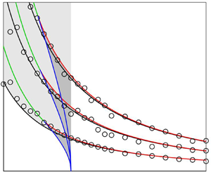
  $1.10$ using the vortex-sheet model are represented in figure 4(a–c) as a function of wavenumber
  $k$ and Strouhal number
  $St_D$. These values are chosen to illustrate the three types of results obtained, respectively, for subsonic Mach numbers below and above
  ${M} \simeq 0.80$ and for supersonic Mach numbers. For each azimuthal mode, waves are allowed for specific values of
  $(k,{St}_D)$. They are classified into different radial modes, with the mode number
  $n_r$ given by the number of antinodes exhibited by the eigenfunction between the jet centreline and the shear layer. The dispersion curves start from a limit point
  $L$ on the line
  $k=-\omega /c_0$, where
  $\omega =2{\rm \pi} f$, at a Strouhal number increasing with the mode number. The waves propagate in the upstream direction when their group velocities
  $v_g=d\omega /dk$ are negative and in the downstream direction when
  $v_g>0$. In what follows, they will be denoted as
  $v_g^-$ waves in the first case and
  $v_g^+$ waves in the second one. The points on the curves where
  $v_g=0$ and
  $dv_g/dk=0$ are marked in order to distinguish between different portions and locate waves with specific characteristics on the dispersion curves. They will be referred to as the stationary and inflection points
  $S$ and
  $I$, respectively. The points
  $S$ also correspond to the saddle points in the complex wavenumber plane whose importance in the emergence of acoustic tones in the potential core of high subsonic jets was highlighted in Towne et al. (Reference Towne, Cavalieri, Jordan, Colonius, Schmidt, Jaunet and Brès2017). At these points, the waves have zero group velocity, do not propagate and are stationary by nature. At points
  $I$, the waves have zero group-velocity dispersion. They are the least dispersive (Whitham Reference Whitham1974) and most coherent waves, and travel without frequency change. This led, for instance, Tam & Ahuja (Reference Tam and Ahuja1990) to assume that they are the most likely to establish stable feedback loops in subsonic jets impinging on a flat plate, which is supported by experimental data for Mach numbers between 0.7 and 0.95 in their paper.

Figure 4. Dispersion relations obtained using the vortex-sheet model for the guided jet waves at (a)  ${M}=0.70$, (b)
  ${M}=0.90$ and (c)
  ${M}=1.10$ for
  $n_{\theta }=0$ (black lines) and
  $n_{\theta }=1$ (grey lines) as a function of
  $k$ and
  ${St}_D$; points
  $L$ (black circles),
  $S_{max}$ (red circles),
  $S_{min}$ (blue circles) and
  $I$ (green circles); dispersion relations of the acoustic waves in a duct for
  $n_{\theta }=0$ (black dashed lines) and
  $n_{\theta }=1$ (grey dashed lines);
  $k=\omega /(u_j-c_0)$ (black dash-dotted lines),
  $k=-\omega /c_0$ (black dotted lines).
For the subsonic Mach numbers  ${M}=0.70$ and 0.90, in figure 4(a,b), the dispersion curves fully stand in the region with negative wavenumbers, between the two straight lines
  $k=-\omega /c_0$ and
  $k=\omega /(u_j-c_0)$ indicating waves with phase and group velocities equal to
  $-c_0$ and
  $u_j-c_0$. The curves are close to the first line near the limit points
  $L$ of the modes and converge towards the second one as the wavenumber tends to
  $-\infty$ and the Strouhal number increases. To further characterize the guided waves, following Towne et al. (Reference Towne, Cavalieri, Jordan, Colonius, Schmidt, Jaunet and Brès2017), the dispersion curves obtained for the acoustic modes in a cylindrical soft duct for
  $n_{\theta }=0$ and
  $1$ are also displayed. They coincide with the dispersion curves of the guided jet modes for high wavenumbers, in absolute value, but progressively deviate from them as one approaches the line
  $k=-\omega /c_0$. Thus, Towne et al. (Reference Towne, Cavalieri, Jordan, Colonius, Schmidt, Jaunet and Brès2017) proposed to separate the modes into two categories, namely the duct-like modes and the free-stream modes. For
  ${M}=0.90$, in figure 4(b), they suggested that the waves belong to free-stream modes between points
  $L$ and
  $S_{max}$, named S2 in their work, and to duct-like modes anywhere else on the dispersion curves. For
  ${M}=0.70$, in figure 4(a), it appears similarly that the waves can be considered as free-stream waves between points
  $L$ and
  $I$ and as duct-like waves to the left of points
  $I$.
$I$.
Regarding the group velocities of the waves, they are always negative for  ${M}=0.70$ in figure 4(a), implying that the waves all propagate in the upstream direction. Given that
  ${St}_D=0$ at the limit point
  $L$ of the first axisymmetric mode,
  $v_g^-$ waves can be found for all frequencies. For
  ${M}=0.90$, in figure 4(b), the group velocities of the waves are negative between points
  $L$ and
  $S_{max}$, positive between
  $S_{max}$ and
  $S_{min}$ and negative again to the left of
  $S_{min}$, where
  $S_{min}$ and
  $S_{max}$ are the stationary points associated, respectively, with the local minimum and the local maximum on the dispersion curves, corresponding to the saddle points S1 and S2 in Towne et al. (Reference Towne, Cavalieri, Jordan, Colonius, Schmidt, Jaunet and Brès2017). Therefore, as for
  ${M}=0.70$,
  $v_g^-$ waves are possible for all frequencies. However,
  $v_g^+$ waves propagating in the downstream direction can also exist, over limited frequency bands ranging between the Strouhal numbers at points
  $S_{min}$ and
  $S_{max}$. These waves vanish below threshold Mach numbers depending on the azimuthal and radial modes. The threshold Mach number is equal to
  ${M}=0.82$ for the first axisymmetric mode and to
  ${M}=0.80$ for the first helical mode, for example, and decreases for higher radial modes.
For the supersonic Mach number  ${M}=1.10$, in figure 4(c), the dispersion curves first extend in the region with negative wavenumbers, to the left of the limit points
  $L$ on the line
  $k=-\omega /c_0$ down to
  ${St}_D=0$, and then continue in the region with positive wavenumbers, tending towards the line
  $k=\omega /(u_j-c_0)$, as illustrated in Morris (Reference Morris2010) for instance. For all modes, the group velocities of the waves are negative from points
  $L$ to
  $S_{max}$ and positive everywhere else. As a result, as for
  ${M}=0.90$, the waves can propagate both in the upstream and the downstream directions. Nevertheless, contrary to the previous case, the
  $v_g^-$ waves are now restricted to very narrow frequency bands ranging between the Strouhal numbers at points
  $L$ and
  $S_{max}$, whereas the
  $v_g^+$ waves are allowed for all frequencies.
Pressure eigenfunctions obtained using the vortex-sheet model for the guided jet mode ( $n_{\theta }=1$,
  $n_r=1$) at
  ${M}=0.70$, 0.90 and 1.10 are shown in figure 5(a–c) between
  $r=0$ and
  $r=1.5r_0$. They are determined at the points
  $L$,
$L$,  $I$,
$I$,  $S_{max}$ and
  $S_{min}$, when available. The first helical mode is considered, but similar trends can be seen for the other azimuthal modes. As reported in previous studies, the waves are essentially confined inside the jet flow and they decay with the radial distance at a rate depending on the point on the dispersion curves. Outside the jet flow, in particular, the wave magnitudes are quite significant at the limit points
  $L$, but much lower at the other points. More precisely, they are approximately two times smaller at the stationary points
  $S_{max}$ for
  ${M}=0.90$ and
  ${M}=1.10$, and 5 times smaller at the inflection point
  $I$ for
  ${M}=0.70$. They are even negligible at the stationary point
  $S_{min}$ for
  ${M}=0.90$, resulting in almost entirely confined waves in that case (Tam & Ahuja Reference Tam and Ahuja1990). These trends are consistent with the classification of the waves into free-stream waves near the line
  $k=-\omega /c_0$ and duct-like waves otherwise. However, the changeover from free-stream to duct-like waves is gradual, which makes it difficult to claim, for some waves such as those found in the vicinity of the points
  $I$ for
  ${M}=0.70$ and
  $S_{max}$ for
  ${M}=0.90$ for instance, whether they are free-stream or duct-like waves.

Figure 5. Pressure eigenfunctions obtained using the vortex-sheet model for the guided jet waves at (a)  ${M}=0.70$, (b)
  ${M}=0.90$ and (c)
  ${M}=1.10$ at points
  $L$ (black lines),
  $S_{max}$ (red lines),
  $S_{min}$ (blue lines) and
  $I$ (green lines) on the dispersion curves of the mode (
 $n_{\theta }=1$,
  $n_r=1$).
To better quantify the amplitude of the waves outside of the jet flow, the magnitudes of the pressure eigenfunctions obtained at  $r=1.5r_0$ for
  $n_{\theta }=0$ and 1 at the Mach numbers of the six jets with tripped boundary layers are represented in figure 6(a–f) as a function of
  ${St}_D$. The
  $v_g^-$ and
  $v_g^+$ waves propagating in the upstream and downstream directions are indicated by solid and dashed lines, respectively, and the points
  $L$,
$L$,  $I$,
$I$,  $S_{max}$ and
  $S_{min}$ are displayed. The variations with the frequency of the magnitude of the
  $v_g^-$ waves from the limit point
  $L$ depend on the Mach number and on the presence of
  $v_g^+$ waves on the curves. For
  ${M}=0.60$ and 0.75, in figure 6(a,b), in the absence of
  $v_g^+$ waves, the magnitude of the
  $v_g^-$ waves decays continuously with the frequency, as was noticed by Jordan et al. (Reference Jordan, Jaunet, Towne, Cavalieri, Colonius, Schmidt and Agarwal2018) also for
  ${M}=0.60$. The decay is slow for
  ${M}=0.60$ but much faster for
  ${M}=0.75$. It is maximum at points
  $I^{\prime }$, which are close to the inflection points
  $I$ for
  ${M}=0.60$ and nearly coinciding with them for
  ${M}=0.75$. For
  ${M}=0.90$, in figure 6(c),
  $v_g^-$ waves are first found between
  $L$ and
  $S_{max}$, and again below
  $S_{min}$ but with an amplitude at least two orders of magnitude lower. Consequently, the magnitudes of the
  $v_g^-$ waves are significant between the Strouhal numbers of
  $L$ and
  $S_{max}$ and negligible for higher frequencies. Finally, for
  ${M}=1.10$, 1.30 and 2, in figure 6(d–f), as the waves are all
  $v_g^+$ waves below the stationary points
  $S_{max}$, the
  $v_g^-$ waves are cut off above the Strouhal numbers of these points. Therefore, each guided jet mode can be regarded as a band-pass filter of the upstream-propagating waves. The filter band-width appears to decrease with the Mach number, and can be approximated by the frequency difference between points
  $L$ and
  $I$ for
  ${M}\leq 0.80$, and points
  $L$ and
  $S_{max}$ for
  ${M}\geq 0.80$. Around the frequencies of
  $I$ or
  $S_{max}$, the filter cutoff is smooth in the first case with a slope steepening with the Mach number, but it is sharp in the second case.

Figure 6. Magnitudes of the pressure eigenfunctions obtained using the vortex-sheet model for the guided jet waves at  $r=1.5r_0$ at (a)
  ${M}=0.60$, (b)
  ${M}=0.75$, (c)
  ${M}=0.90$ (d)
  ${M}=1.10$, (e)
  ${M}=1.30$ and (f)
  ${M}=2$ as a function of
  ${St}_D$: upstream-propagating (solid lines) and downstream-propagating (dashed lines) waves for
  $n_{\theta }=0$ (black) and
  $n_{\theta }=1$ (grey); points
  $L$ (black circles),
  $S_{max}$ (red circles),
  $S_{min}$ (blue circles) and
  $I$ (green circles) on the dispersion curves; points
  $I^{\prime }$ (filled green circles) of maximum rate of decrease. Only the waves with
  $k\leq 0$ are considered for supersonic Mach numbers.
The dispersion relations of the guided jet waves allow us to determine the allowable frequency bands for the  $v_g^-$ waves propagating in the upstream direction (Tam & Norum Reference Tam and Norum1992). The bands predicted using the vortex-sheet model between
  ${M}=0.50$ and 2 for the first five radial modes for
  $n_{\theta }=0$ and 1 are represented as a function of the Mach and the Strouhal number in figure 7(a,b), along with the points
  $L$,
$L$,  $S_{max}$,
  $S_{min}$,
  $I$ and
  $I^{\prime }$ defined above. The bands are highlighted in two shades of grey, depending on the presence of
  $v_g^+$ waves simultaneously with the
  $v_g^-$ waves. In the dark-grey regions,
  $v_g^-$ and
  $v_g^+$ waves are both permitted, making acoustic resonance possible in the jet potential core (Towne et al. Reference Towne, Cavalieri, Jordan, Colonius, Schmidt, Jaunet and Brès2017). In the light-grey ones, on the contrary, only
  $v_g^-$ waves can be found. For subsonic Mach numbers, the upstream-propagating waves can exist at all frequencies for
  $n_{\theta }=0$ and over a wide range of frequencies for
  $n_{\theta }=1$. As the Mach number decreases, the inflection points
  $I$ gradually move away from the points
  $I^{\prime }$ of maximum decay of the eigenfunction magnitude outside of the jet. They remain, however, very close to each other nearly down to
  ${M}=0.60$. For supersonic Mach numbers, as mentioned previously, the upstream-propagating waves are restricted to bands narrowing with the Mach number. For a given Mach number, these bands are much smaller for
  $n_{\theta }=1$ than for
  $n_{\theta }=0$, yielding extremely thin bands for
  $n_{\theta }=1$ at
  ${M}=2$ for example. As the radial mode number increases, the bands are also smaller for
  $n_{\theta }=0$ but larger for
  $n_{\theta }=1$.

Figure 7. Allowable Strouhal number ranges obtained using the vortex-sheet model for the upstream-propagating guided jet waves with (dark grey shading) and without (light grey shading) downstream-propagating guided waves for (a)  $n_{\theta }=0$ and (b)
  $n_{\theta }=1$ as a function of
  ${M}$; points
  $L$ (black lines),
  $S_{max}$ (red lines),
  $S_{min}$ (blue lines),
  $I$ (green lines) and
  $I^{\prime }$ (green dashed lines) on the dispersion curves. The first five radial modes are shown.
3.2. Guided jet waves for the azimuthal modes  $n_{\theta }\geq 2$

The properties of the guided jet waves associated with the azimuthal modes  $n_{\theta }\geq 2$, whose contributions to the emergence of acoustic tones in the potential core and the near field of jets have not been discussed in the literature to the best of the author's knowledge, are briefly examined in this section. For that, the dispersion relations of the waves have been calculated using the vortex-sheet model for
  $n_{\theta }=2$ to 8 over the Mach number range considered in the present work.
The dispersion relations obtained at  ${M}=0.70$,
  $0.90$ and
  $1.10$ for
  $n_{\theta }=2$ to 5 are represented in figure 8(a–c) as a function of
  $k$ and
  $St_D$, along with those for
  $n_{\theta }=0$ and 1. The results for
  $n_{\theta }=6$ to 8 are not plotted, for clarity. For each azimuthal mode,
  $n_{\theta }$ is indicated on the curve for the first radial mode. At a higher azimuthal mode, the dispersion curves are found for higher Strouhal numbers, but their shapes do not change much. As a result, they are essentially aligned with each other, and are sometimes very similar. The latter can be observed, for instance, for the solid black curve related to the second radial axisymmetric mode and the dashed black curve of the first radial mode for
  $n_{\theta }=2$, and for the solid black curve of the third radial axisymmetric mode and the dash-dotted grey curve of the first radial mode for
  $n_{\theta }=5$. Differences between the dispersion relations can, however, be noted in the vicinity of the line
  $k=-\omega /c_0$. The portion of the curves near that line is narrower as the azimuthal mode number increases. This leads to limit points
  $L$ closer to the inflection points
  $I$ for
  ${M}= 0.70$ in figure 8(a) and to the stationary points
  $S_{max}$ for
  ${M}=0.90$ and
  $1.10$ in figure 8(b,c). There are even no points
  $S_{max}$ at
  ${M}=0.90$ for
  $n_{\theta }\geq 3$ and at
  ${M}=1.10$ for
  $n_{\theta }\geq 2$. In these cases, the curves have a positive slope immediately to the left of the limit points
  $L$, suggesting that free-stream upstream-propagating guided jet waves cannot exist.

Figure 8. Dispersion relations obtained using the vortex-sheet model for the guided jet waves at (a)  ${M}=0.70$, (b)
  ${M}=0.90$ and (c)
  ${M}=1.10$ for
  $n_{\theta }=$ 0 (black lines), 1 (grey lines), 2 (black dashed lines), 3 (grey dashed lines), 4 (black dash-dotted lines) and 5 (grey dash-dotted lines) as a function of
  $k$ and
  ${St}_D$; points
  $L$ (black circles),
  $S_{max}$ (red circles),
  $S_{min}$ (blue circles) and
  $I$ (green circles);
  $k=-\omega /c_0$ (black dotted lines). For each azimuthal mode,
  $n_{\theta }$ is indicated on the dispersion curve for the first radial mode. Only the part with
  $k\leq 0$ is shown for
  ${M}=1.10$.
The allowable frequency bands obtained using the vortex-sheet model between  ${M}=0.5$ and 2 for the first five radial upstream-propagating wave modes for
  $n_{\theta }=2$, 3 and 4 are represented as a function of the Mach and the Strouhal number in figure 9(a–c). They resemble those obtained for
  $n_{\theta }=0$ and 1 in figure 7(a,b). Compared with these two modes, however, the inflection points
  $I$ and the stationary points
  $S_{max}$ are nearer to the limit points
  $L$, providing narrower bands. The bands even subsist only up to threshold Mach numbers, indicated by red asterisks, above which there is no stationary point
  $S_{max}$ on the dispersion curves. The threshold values decrease with the azimuthal mode number and are, for example, equal to
  ${M} = 1.09$, 0.86 and 0.78 for the radial modes
  $n_r=1$ for
  $n_{\theta }=2$, 3 and 4. They also increase with the radial mode number and vary, for instance, from
  ${M} =1.09$ for
  $n_r=1$ up to
  $1.86$ for
  $n_r=5$ in figure 9(a) for
  $n_{\theta }=2$. Again, the vortex-sheet model predicts the non-existence of free-stream upstream-propagating waves for the azimuthal modes
  $n_{\theta }\geq 2$ at sufficiently high Mach numbers. The dispersion curves of the guided jet waves being sensitive to the thickness of the mixing layer, as shown theoretically in Tam & Ahuja (Reference Tam and Ahuja1990) for a Mach number of 0.8 and numerically in Bogey & Gojon (Reference Bogey and Gojon2017) for a Mach number of 1.5, one may wonder whether this will be true for jets with mixing layers of finite thickness, such as those simulated in the present study.

Figure 9. Allowable Strouhal number ranges obtained using the vortex-sheet model for the upstream-propagating guided jet waves with (dark grey shading) and without (light grey shading) downstream-propagating guided waves for (a)  $n_{\theta }=2$, (b)
  $n_{\theta }=3$ and (c)
  $n_{\theta }=4$ as a function of
  ${M}$; points
  $L$ (black lines),
  $S_{max}$ (red lines),
  $S_{min}$ (blue lines) and
  $I$ (green lines) on the dispersion curves; threshold Mach numbers for the presence of
  $S_{max}$ points (red asterisks). The first five radial modes are shown.
4. Simulation results
4.1. Snapshots and flow properties
The flow and near pressure fields of the jets with tripped boundary layers are briefly presented. For conciseness, those obtained for the jets with untripped boundary layers are not shown. In short, these jets exhibit roll-ups and pairings of vortical structures (Winant & Browand Reference Winant and Browand1974) in their initially fully laminar mixing layers, which occur more rapidly and at a higher frequency as the boundary-layer thickness decreases (Bogey & Bailly Reference Bogey and Bailly2010; Bogey Reference Bogey2018), and farther downstream as the Mach number increases in agreement with linear stability analyses (Michalke Reference Michalke1984; Morris Reference Morris2010). The vortex pairings generate strong acoustic waves in the downstream direction (Colonius, Lele & Moin Reference Colonius, Lele and Moin1997).
Snapshots of the vorticity and pressure fields obtained downstream of the nozzle-exit section for the jets with tripped boundary layers at  ${M}=0.60$,
  $0.75$,
  $0.90$,
  $1.30$ and
  $2$ are provided in figure 10(a–e). Due to the highly disturbed exit flow conditions, turbulence is found just downstream of the nozzle, no vortex pairing can be easily detected in the shear layers, and fine-scale structures and high-frequency sound waves can be seen. In the pressure fields, fluctuations of hydrodynamic nature are visible just outside of the jets (Arndt, Long & Glauser Reference Arndt, Long and Glauser1997) and waves are observed in the potential cores (Towne et al. Reference Towne, Cavalieri, Jordan, Colonius, Schmidt, Jaunet and Brès2017). For a higher jet velocity, the shear layers develop faster and Mach waves are radiated due to the convection of the flow structures at a supersonic speed. Footprints of shock cells can also be detected in the cores of the supersonic jets despite ambient pressure being imposed at the inlet of the pipe nozzle.

Figure 10. Snapshots in the  $(z,r)$ plane of vorticity norm between
  $r=0.5r_0$ and
  $r=1.5r_0$ and of pressure fluctuations otherwise for the jets with tripped boundary layers at (a)
  ${M}=0.60$, (b)
  ${M}=0.75$, (c)
  ${M}=0.90$, (d)
  ${M}=1.30$ and (e)
  ${M}=2$. The colour scales range between
  $\pm 20u_j/r_0$ and (a)
  $\pm 3.5\times 10^{-3} p_0$, (b)
  $\pm 4.25\times 10^{-3} p_0$, (c)
  $\pm 5.5\times 10^{-3} p_0$, (d)
  $\pm 1.3\times 10^{-2} p_0$ and (e)
  $\pm 2.5\times 10^{-2} p_0$, from blue to red.
The effects of the Mach number on the jet flow development are illustrated by the variations of the shear-layer momentum thickness, of the r.m.s. values of axial velocity at  $r=r_0$ and of the centreline mean axial velocity in figure 11(a–c). As the Mach number increases, the shear layers spread more slowly in figure 11(a) due to the lower growth rates of instability waves (Michalke Reference Michalke1984) and to compressibility effects (Brown & Roshko Reference Brown and Roshko1974). As expected (Lau et al. Reference Lau, Morris and Fisher1979), this leads to longer potential cores in figure 11(c), ending at
  $z_c=13r_0$ for
  ${M}=0.60$,
  $z_c=14.8r_0$ for
  ${M}=0.90$,
  $z_c=17.8r_0$ for
  ${M}=1.30$ and
  $z_c=23.4r_0$ for
  ${M}=2$ for instance. In that figure, the centreline mean velocity profiles exhibit oscillations in the core of the supersonic jets, but they are quite small, indicating that the shock-cell structures are very weak and that the jets are nearly ideally expanded at the nozzle exit. Finally, in figure 11(b), the profiles of turbulence intensities in the mixing layers are quite flat due to the high level of velocity fluctuations at the nozzle exit (Bogey et al. Reference Bogey, Marsden and Bailly2012), and reach peak values decreasing from 17 % for
  ${M}=0.60$ down to 15 % for
  ${M}=2$.

Figure 11. Axial variations of (a) the shear-layer momentum thickness, (b) the r.m.s. values of axial velocity at  $r=r_0$ and (c) the mean axial velocity at
  $r=0$ for the jets with tripped boundary layers at
  ${M}=$ 0.60 (black lines),
  $0.75$ (red lines),
  $0.90$ (blue lines),
  $1.10$ (black dashed lines),
  $1.30$ (red dashed lines) and
  $2$ (blue dashed lines).
4.2. Acoustic tones for the jets at a Mach number of 0.90
The presence and properties of acoustic tones in the jet potential core, in the near-nozzle region and in the pressure far field are first examined for the six jets at  ${M}=0.90$ in figure 1, with particular emphasis on the jet with tripped boundary layers.
4.2.1. Tones in the jet potential core
In order to shed light on the waves in the jets, a space–time Fourier transform has been applied to the pressure fluctuations inside the jet potential core for azimuthal modes  $n_{\theta }=0$ and 1, as in previous work on free, impinging and screeching jets (Bogey & Gojon Reference Bogey and Gojon2017; Towne et al. Reference Towne, Cavalieri, Jordan, Colonius, Schmidt, Jaunet and Brès2017, Reference Towne, Schmidt and Brès2019; Gojon et al. Reference Gojon, Bogey and Mihaescu2018), but also for modes
  $n_{\theta }=2$ to 8. The pressure fluctuations are taken at a fixed radial position, depending on the azimuthal mode, from the nozzle exit at
  $z=0$ down to
  $z=0.7z_c$. The latter position allows us to reduce the contributions of the pressure disturbances of aerodynamic nature, particularly significant around the end of the potential core, while permitting a substantial spatial extent in the axial direction.
The spectra obtained for the jets with tripped boundary layers for  $n_{\theta }=0$ to 5 are represented in figure 12(a–f) as a function of wavenumber and Strouhal number. For positive wavenumbers, strong components lie near the line
  $k=\omega /(0.75u_j)$. They correspond to the footprints left in the jet potential core by the shear-layer turbulent structures convected by the flow. For negative wavenumbers, high levels appear along bands near the dispersion curves predicted for the guided jet waves using the vortex-sheet model. This is clearly visible for
  $n_{\theta }=0$ and 1, as in Towne et al. (Reference Towne, Cavalieri, Jordan, Colonius, Schmidt, Jaunet and Brès2017) also for a Mach number 0.9 jet, as well as for higher azimuthal modes. Differences can be noted between the bands and the dispersion curves. They are less important in the spectra for the untripped jets with thinner boundary layers, not shown for brevity. Therefore, they can be attributed to the assumption of an infinitely thin shear layer in the vortex-sheet model. In agreement with previous studies (Tam & Ahuja Reference Tam and Ahuja1990; Bogey & Gojon Reference Bogey and Gojon2017), the bands are slightly above the dispersion curves far from the line
  $k=-\omega /c_0$. Near the line, the opposite trend is observed for
  $n_{\theta }=0$ to 2 in figure 12(a–c). In this zone, the bands have larger portions with a negative slope than the dispersion curves, yielding waves with a negative group velocity over wider frequency ranges. This is especially true for
  $n_{\theta }=3$ to 5 in figure 12(d–f), for which upstream-propagating waves are found near
  $k=-\omega /c_0$ for all radial modes, contrary to the model prediction. In that case, they are restricted to Strouhal numbers around that of the limit points
  $L$ given by the model. Moreover, the bands are thicker as the azimuthal mode number increases. In the bands, the energy is rather evenly distributed and no peak can be detected, unlike the results for impinging and screeching jets (Bogey & Gojon Reference Bogey and Gojon2017; Gojon et al. Reference Gojon, Bogey and Mihaescu2018) for instance. However, the energy levels are, overall, highest between the Strouhal numbers of the two stationary points
  $S_{min}$ and
  $S_{max}$, as pointed out by Towne et al. (Reference Towne, Cavalieri, Jordan, Colonius, Schmidt, Jaunet and Brès2017). In most cases, the maximum levels even appear mainly located between
  $S_{min}$ and
  $S_{max}$ where the waves propagate in the downstream direction.

Figure 12. Frequency–wavenumber spectra of pressure fluctuations in the potential core of the jet at  ${M}=0.90$ with tripped boundary layers at (a)
  $r=0$ for
  $n_{\theta }=0$, (b)
  $r=0.2r_0$ for
  $n_{\theta }=1$, (c)
  $r=0.3r_0$ for
  $n_{\theta }=2$, (d)
  $r=0.3r_0$ for
  $n_{\theta }=3$, (e)
  $r=0.4r_0$ for
  $n_{\theta }=4$ and (f)
  $r=0.4r_0$ for
  $n_{\theta }=5$ as a function of
  $(kD,{St}_D)$; dispersion curves of the guided jet waves (black lines), points
  $L$ (black circles),
  $S_{max}$ (red circles) and
  $S_{min}$ (blue circles);
  $k=-\omega /c_0$ (black dashed lines),
  $k=\omega /(0.75u_j)$ (black dash-dotted lines). The grey-scale levels spread over 25 dB.
Spectra of pressure fluctuations obtained for  $n_{\theta }=0$ to 5 in the potential core of the jets with tripped boundary layers and with untripped boundary layers with
  $\delta _{BL}=0.025r_0$ are plotted in figure 13(a–f) as a function of
  ${St}_D$. To be consistent with the frequency–wavenumber spectra of figure 12, they are computed at the same radial positions, by averaging between
  $z=0$ and
  $z=0.7 z_c$. The allowable frequency ranges predicted using the vortex-sheet model for the upstream-propagating guided jet waves are displayed using the same colour code as in figures 7 and 9. To avoid an overlapping of the dark-grey bands, in which upstream-propagating but also downstream-propagating waves can exist, only the bands for the first four radial guided jet modes are represented for
  $n_{\theta }=0$. In the same way, only the bands for
  $n_r=1-3$ and
  $n_r=1-2$ are shown for
  $n_{\theta }=1,2$ and
  $n_{\theta }=3-5$, respectively. For all azimuthal modes, despite the presence of strong broadband aerodynamic components, visible in the spectra of figure 12 for positive wavenumbers, large acoustic peaks emerge in the spectra. They lie exclusively within the dark-grey bands, indicating that they are closely linked to the presence of
  $v_g^+$ guided jet waves. These results are in line with the findings of Towne et al. (Reference Towne, Cavalieri, Jordan, Colonius, Schmidt, Jaunet and Brès2017), who demonstrated the possibility of resonant interactions between the former waves and
  $v_g^-$ guided waves in high subsonic jets between the frequencies of the stationary points
  $S_{min}$ and
  $S_{max}$ for
  $n_{\theta }=0$ and 1. In the present work, these interactions are found to be possible for higher azimuthal modes. On the basis of the frequency–wavenumber spectra of figure 12, two types of resonances can occur (Towne et al. Reference Towne, Cavalieri, Jordan, Colonius, Schmidt, Jaunet and Brès2017). The first one involves
  $v_g^+$ and
  $v_g^-$ duct-like waves located on both sides of points
  $S_{min}$ and the second one happens between
  $v_g^+$ duct-like and
  $v_g^-$ free-stream waves around points
  $S_{max}$.

Figure 13. Sound pressure levels in the potential core of the jets at  ${M}=0.90$ with tripped boundary layers (black lines) and with untripped boundary layers with
  $\delta _{BL}=0.025r_0$ (red lines) at (a)
  $r=0$ for
  $n_{\theta }=0$, (b)
  $r=0.2r_0$ for
  $n_{\theta }=1$, (c)
  $r=0.3r_0$ for
  $n_{\theta }=2$, (d)
  $r=0.3r_0$ for
  $n_{\theta }=3$, (e)
  $r=0.4r_0$ for
  $n_{\theta }=4$ and (f)
  $r=0.4r_0$ for
  $n_{\theta }=5$ as a function of
  ${St}_D$; allowable ranges for the upstream-propagating guided jet waves with (dark grey shading) and without (light grey shading) downstream-propagating guided waves for (a)
  $n_r=1-4$, (b,c)
  $n_r=1-3$ and (d–f)
  $n_r=1-2$.
4.2.2. Tones in the jet near-nozzle region
To identify which of the guided jet waves have a significant radial support outside of the jets, a space–time Fourier transform has been applied to the pressure fluctuations at  $r=1.1r_0$, between
  $z=0$ and
  $z=0.7z_c$ as previously in the potential core, for
  $n_{\theta }=0$ to 8. The spectra for
  $n_{\theta }=0$ to 5 are represented in figure 14(a–f) as a function of
  $k$ and
  ${St}_D$ for
  $k\leq 0$ only. Strong components of aerodynamic nature are observed near
  $k=0$ for low Strouhal numbers due to the proximity of the shear layer. In spite of this, spots of high levels are found for all azimuthal modes in the vicinity of the dispersion curves predicted for the guided jet waves using the vortex-sheet model. With respect to the elongated bands obtained in the in-core spectra of figure 12, the spots do extend along the curves but are restricted to very limited parts. Their levels are highest close to the line
  $k=-\omega /c_0$, rapidly decrease farther from it and are negligible to the left of the local maximum point. Therefore, the waves located between the limit points
  $L$ and the stationary points
  ${S}_{max}$ of the dispersion curves, i.e. the so-called free-stream waves in Towne et al. (Reference Towne, Cavalieri, Jordan, Colonius, Schmidt, Jaunet and Brès2017), are detected just outside of the jets, whereas the other, duct-like, waves are not. The frequency ranges of the free-stream waves also appear to be narrower at a higher azimuthal mode. These results are in agreement with the variations of the eigenfunction magnitude of the guided jet waves outside of the shear layer in figures 5(b) and 6(c), and with the merging of points
  $L$ and
  ${S}_{max}$ as the azimuthal mode number increases in figures 7 and 9 for
  ${M}=0.90$. Given their negative group velocities, the free-stream waves propagate in the upstream direction, and can be expected to mark the pressure spectra in the near-nozzle region.

Figure 14. Frequency–wavenumber spectra of pressure fluctuations of the jet at  ${M}=0.90$ with tripped boundary layers at
  $r=1.1r_0$ for (a)
  $n_{\theta }=0$, (b)
  $n_{\theta }=1$, (c)
  $n_{\theta }=2$, (d)
  $n_{\theta }=3$, (e)
  $n_{\theta }=4$ and (f)
  $n_{\theta }=5$ as a function of
  $(kD,{St}_D)$; dispersion curves of the guided jet waves (black lines), points
  $L$ (black circles),
  $S_{max}$ (red circles) and
  $S_{min}$ (blue circles);
  $k=-\omega /c_0$ (black dashed lines). The grey-scale levels spread over 25 dB. Only
  $k\leq 0$ is shown.
The spectra of pressure fluctuations computed near the nozzle exit at  $z=0$ and
  $r=1.5r_0$ for the jets with tripped boundary layers and with untripped boundary layers with
  $\delta _{BL}=0.025r_0$ are represented in figure 15(a,b) as a function of
  ${St}_D$. The contributions of the first six azimuthal modes are also depicted. Tonal peaks emerge in the full spectra as well as for the azimuthal modes. They are very similar to those found in the near-nozzle spectra reported in Suzuki & Colonius (Reference Suzuki and Colonius2006), Towne et al. (Reference Towne, Cavalieri, Jordan, Colonius, Schmidt, Jaunet and Brès2017) and Brès et al. (Reference Brès, Jordan, Jaunet, Le Rallic, Cavalieri, Towne, Lele, Colonius and Schmidt2018) for jets at the same Mach number as the present jets but at Reynolds numbers
  $Re_D\simeq 10^6$. They are stronger and narrower for the jet with untripped boundary layers than for the other one. However, the peak frequencies are almost identical in the two cases. For a given azimuthal mode, the first peak falls very near the dash-dotted line indicating the Strouhal number of point
  ${S}_{max}$, or
  $L$ in the absence of
  ${S}_{max}$, obtained on the dispersion curves for the radial guided jet mode
  $n_r=1$ using the vortex-sheet model. This supports that the peaks are due to the upstream-propagating waves highlighted in figure 14. Regarding the full spectra, the first, second and third peaks at
  ${St}_D\simeq 0.4$,
  $0.6$ and 1 coincide with the first peaks of modes
  $n_{\theta }=0$, 1 and 2 in red, blue and green, respectively. The fourth peak corresponds to the first peak of mode
  $n_{\theta }=3$ in magenta, enhanced by the second peak of mode
  $n_{\theta }=1$ in blue. The higher peaks also consist of combinations of peaks of different modes, for instance modes
  $n_{\theta }=2$ and 4 for the fifth peak and modes
  $n_{\theta }=1$, 3 and 5 for the sixth peak. The complex structure of the peaks can be explained by the great resemblance, and quasi superposition in some instances, of the dispersion curves for different azimuthal modes, discussed in § 3.2 based on figure 8. This issue was mentioned by Suzuki & Colonius (Reference Suzuki and Colonius2006) who remarked that the frequency of the first peak of mode
  $n_{\theta }=2$ is nearly the same as that of the second peak of mode
  $n_{\theta }=0$ in their experimental spectra.

Figure 15. Sound pressure levels obtained at  $z=0$ and
  $r=1.5r_0$ for the jets at
  ${M}=0.90$ (a) with tripped boundary layers and (b) with untripped boundary layers with
  $\delta _{BL}=0.025r_0$ as a function of
  ${St}_D$: full spectra (black lines) and
  $n_{\theta }=$ 0 (red lines), 1 (blue lines), 2 (green lines), 3 (magenta lines), 4 (yellow lines) and 5 (light blue lines). Dash-dotted lines: Strouhal numbers at points
  $S_{max}$ or
  $L$ on the dispersion curves for the guided jet modes (
 $n_{\theta }$,
  $n_r=1$) using the same colours as for the solid lines.
The spectra calculated at  $z=0$ and
  $r=1.5r_0$ for the jets with tripped boundary layers and untripped boundary layers with
  $\delta _{BL}=0.025r_0$ for modes
  $n_{\theta }=0$ to 5 are plotted in figure 16(a–f) as a function of
  $St_D$. The allowable ranges for the upstream-propagating guided jet waves according to the vortex-sheet model are represented in grey as in figure 13. The frequency ranges of the free-stream waves between points
  $L$ and
  $S_{max}$ on the dispersion curves are also indicated by oblique hatching, when possible. Compared with the peaks obtained in the potential core in figure 13, the near-nozzle peaks are narrower and exhibit a sharper decrease on the right side of the stationary points
  ${S}_{max}$. Moreover, instead of fully filling the dark-grey bands where
  $v_g^-$ and
  $v_g^+$ guided jet waves can both exist, they appear limited to the hatched bands. This trend is clearly observed for modes
  $n_{\theta }\geq 1$ in figure 16(b–f), for which points
  $L$ and
  $S_{max}$ are very close or superimposed on the dispersion curves, which gives rise to very tonal peaks. The present results are in agreement with the eigenfunctions of figure 5(b) and the transfer functions of 6(c). They show that the near-nozzle peaks are mainly related to the free-stream guided jet waves. In particular, it appears that among the resonant interactions possibly occurring between
  $v_g^-$ and
  $v_g^+$ guided waves in the jet potential core, only those involving
  $v_g^-$ free-stream waves can contribute significantly to the near-nozzle pressure field. Given that the peak levels are higher at point
  $S_{max}$ than at point
  $L$ when the two points are sufficiently distinct from each other, as for mode (
 $n_{\theta }=0$,
  $n_r=2$) in figure 16(a) and for mode (
 $n_{\theta }=1$,
  $n_r=1$) in figure 16(b), this may be especially true for the waves resonating around the stationary point
  ${S}_{max}$.

Figure 16. Sound pressure levels obtained at  $z=0$ and
  $r=1.5r_0$ for the jets at
  ${M}=0.90$ with tripped boundary layers (black lines) and with untripped boundary layers with
  $\delta _{BL}=0.025r_0$ (red lines) for (a)
  $n_{\theta }=0$, (b)
  $n_{\theta }=1$, (c)
  $n_{\theta }=2$, (d)
  $n_{\theta }=3$, (e)
  $n_{\theta }=4$ and (f)
  $n_{\theta }=5$ as a function of
  ${St}_D$; allowable ranges for the upstream-propagating guided jet waves with (dark grey shading) and without (light grey shading) downstream-propagating guided waves and between the
  ${St}_D$ at points
  $L$ and
  $S_{max}$ (hatched) for (a)
  $n_r=1-4$, (b–c)
  $n_r=1-3$ and (d–f)
  $n_r=1-2$,
  ${St}_D$ at points
  $L$ on the dispersion curves (black dash-dotted lines).
The Strouhal numbers of the peaks obtained for the six jets at  ${M}=0.90$ in the spectra at
  $z=0$ and
  $r=1.5r_0$ for
  $n_{\theta }=0$, 1 and 2 are represented in figure 17(a–c) as a function of boundary-layer thickness
  $\delta _{BL}$ at the nozzle-pipe inlet. The allowable bands predicted for the upstream-propagating guided jet waves using the vortex-sheet model, as well as the points
  $L$,
$L$,  $S_{max}$ and
  $S_{min}$ on the dispersion curves given by the model, are also displayed. Over the wide range of boundary-layer thicknesses considered, the peak Strouhal numbers do not vary appreciably despite the ratio of 16 between the largest and the smallest values of
  $\delta _{BL}$. This is in line with the experimental results of Zaman & Fagan (Reference Zaman and Fagan2019) for two jets with boundary-layer thicknesses differing by a factor of 3. In the same way, the peak frequencies are very similar for tripped and untripped boundary layers, as was the case for the two initially laminar and turbulent jets computed by Brès et al. (Reference Brès, Jordan, Jaunet, Le Rallic, Cavalieri, Towne, Lele, Colonius and Schmidt2018). For all jets, even for the one with
  $\delta _{BL}=0.4r_0$ for which the vortex-sheet model is a very rough approximation, the peaks are located between the points
  $L$ and
  $S_{max}$, or near the point
  $L$ when
  $S_{max}$ does not exist. These results provide further evidence about the links between the near-nozzle peaks and the free-stream guided jet waves. In the zones between points
  $L$ and
  $S_{max}$, the peaks are closer to the second point than to the first one for the first two radial modes for
  $n_{\theta }=0$ in figure 17(a). This again supports the possible contributions of waves resonating around the stationary point
  $S_{max}$ to the near-nozzle pressure fields.

Figure 17. Peak Strouhal numbers in the spectra of pressure fluctuations at  $z=0$ and
  $r=1.5r_0$ for the jets at
  ${M}=0.90$ with tripped (filled black circles) and untripped (black circles) boundary layers for (a)
  $n_{\theta }=0$, (b)
  $n_{\theta }=1$ and (c)
  $n_{\theta }=2$ as a function of
  $\delta _{BL}/r_0$; allowable ranges for the upstream-propagating guided jet waves with (dark grey shading) and without (light grey shading) downstream-propagating guided waves,
  ${St}_D$ at points
  $L$ (black dash-dotted lines),
  $S_{max}$ (red lines) and
  $S_{min}$ (blue lines) on the dispersion curves.
The sensitivity of the near-nozzle acoustic peaks to the jet initial conditions is examined by comparing some properties of the near-nozzle peaks obtained for the six jets at  ${M}=0.90$. Only the peaks associated with the guided jet modes
  $n_r=1$ for
  $n_{\theta }=0$, 1 and 2 are considered. The peak intensities are depicted in figure 18(a). They are lower for the jet with tripped boundary layers than for the jets with untripped ones, and for the latter jets, they grow with the boundary-layer thickness except for
  $\delta _{BL}\geq 0.2r_0$. Thus, overall, the more noise generated by the jets (Bogey & Bailly Reference Bogey and Bailly2010; Bogey Reference Bogey2018), the higher the levels of the near-nozzle acoustic peaks.

Figure 18. Near-nozzle peaks for the jets at  ${M}=0.90$ with tripped (filled circles) and untripped (circles) boundary layers for the radial modes
  $n_r=1$ of the guided jet waves for
  $n_{\theta }=0$ (red),
  $n_{\theta }=1$ (blue) and
  $n_{\theta }=2$ (green): (a) peak levels, (b) ratio between the peak levels and the minimum values for higher
  ${St}_D$ and (c) peak widths as a function of
  $\delta _{BL}/r_0$. Dash-dotted lines:
  ${\rm \Delta} {St}_D$ between points
  $S_{max}$ and
  $L$ using the above colours for
  $n_{\theta }$.
In order to quantify the degree of emergence of the peaks, the ratios between the peak levels and the first minimum values reached for a higher frequency are plotted in figure 18(b). As for the peak intensities, they are minimum for the jet with tripped boundary layers and are higher as the boundary layer is thicker for the initially fully laminar jets. Therefore, the near-nozzle peaks are more prominent for the jets with mixing layers containing stronger large-scale coherent structures, and inversely weaker fine-scale turbulent structures, yielding a weaker broadband noise in the upstream direction.
Finally, the peak widths at half of maximum are given in figure 18(c). They increase with the boundary-layer thickness. This trend can be attributed to the effects of the shear-layer thickness on the dispersion curves of the guided jet waves near the line  $k=-\omega /c_0$ (Tam & Ahuja Reference Tam and Ahuja1990; Bogey & Gojon Reference Bogey and Gojon2017). Indeed, as mentioned in § 4.2.1 and illustrated by the frequency–wavenumber spectra of figure 12, the free-stream guided jet waves are obtained over wider frequency ranges for a thicker shear layer. In that case, the band-pass filtering of the upstream-propagating waves by the guided jet modes has a larger width. For comparison, the widths estimated as the frequency differences between points
  $L$ and
  $S_{max}$ on the dispersion curves using the vortex-sheet model for modes (
 $n_{\theta }=1$,
  $n_r=1$) and (
 $n_{\theta }=2$,
  $n_r=1$) are shown in figure 18(c). A fairly good agreement is found with the peak widths for
  $n_{\theta }=1$. For
  $n_{\theta }=2$, the peak width is underestimated by the model, which is expected due to the discrepancies between the numerical and theoretical dispersion curves near
  $k=-\omega /c_0$ in figure 12(c).
4.2.3. Tones in the jet acoustic far field
The LES near-field fluctuations obtained for the jet at  ${M}=0.90$ with tripped boundary layers have been propagated to the far field using an in-house OpenMP-based solver of the isentropic linearized Euler equations in cylindrical coordinates based on the same numerical methods as the LES. Two calculations are performed as in previous studies (Bogey & Sabatini Reference Bogey and Sabatini2019; Bogey Reference Bogey2021). They are carried out from the velocity and pressure fluctuations recorded during time
  $T=3000r_0/u_j$ at
  $r=15r_0$ and at
  $z=-1.5r_0$ and
  $z=L_z=40r_0$ at a sampling frequency corresponding to a Strouhal number of
  ${St}_D=12.8$. They allow us to compute the pressure waves radiated at a distance of
  $150 r_0$ from the nozzle exit, where far-field acoustic conditions are expected to apply (Ahuja, Tester & Tanna Reference Ahuja, Tester and Tanna1987; Viswanathan Reference Viswanathan2010), between the angles
  $\phi =15^{\circ }$ and
  $165^{\circ }$ relative to the jet direction. Grids containing up to
  $1.6 \times 10^9$ points with a uniform mesh spacing of
  $0.075 r_0$ in the axial and radial directions and
  $N_{\theta }=256$ points in the azimuth are used. This mesh spacing, leading to
  ${St}_D=5.9$ for an acoustic wave discretized by five points per wavelength, is identical to that in the LES near pressure field. The sound pressure spectra thus determined at six angles
  $\phi$ between
  $30^{\circ }$ and
  $165^{\circ }$ are represented in figure 19(a–f) as a function of
  ${St}_D$. The contributions of modes
  $n_{\theta }=0$ to 8 are also shown. Because of the different shapes of the spectra (Mollo-Christensen, Kolpin & Martucelli Reference Mollo-Christensen, Kolpin and Martucelli1964; Tam Reference Tam1998), the level axis ranges from 74 up to 116 dB/
 ${St}_D$ in figure 19(a) for
  $\phi =30^{\circ }$, but only up to 104 dB/
 ${St}_D$ in figure 19(b) for
  $\phi =60^{\circ }$ and to 98 dB/
 ${St}_D$ in figure 19(c–f) for
  $\phi \geq 90^{\circ }$.

Figure 19. Sound pressure levels obtained for the jet at  ${M}=0.90$ with tripped boundary layers at
  $150r_0$ from the nozzle exit for (a)
  $\phi =30^{\circ }$, (b)
  $\phi =60^{\circ }$, (c)
  $\phi =90^{\circ }$, (d)
  $\phi =135^{\circ }$, (e)
  $\phi =150^{\circ }$ and (f)
  $\phi =165^{\circ }$ as a function of
  ${St}_D$: full spectra (black lines) and
  $n_{\theta }=$ 0 (red lines), 1 (blue lines), 2 (green lines), 3 (magenta lines), 4 (yellow lines), 5 (light blue lines), 6, 7 and 8 (grey lines). Dash-dotted lines: Strouhal numbers at points
  $S_{max}$ or
  $L$ on the dispersion curves for the guided jet modes (
 $n_{\theta }$,
  $n_r=1$) using the same colours as for the solid lines; measurements of Bridges & Brown (Reference Bridges and Brown2005) for an isothermal jet at
  ${M}=0.9$ and
  ${Re}_D=10^6$ (black triangles).
In the downstream and sideline directions, in figure 19(a–c), the pressure spectra exhibit the characteristics typically found in the far field of subsonic jets. The axisymmetric mode is dominant in the downstream direction and is soon overwhelmed by modes  $n_{\theta }=1$ and 2 as the radiation angle increases (Juvé, Sunyach & Comte-Bellot Reference Juvé, Sunyach and Comte-Bellot1979; Cavalieri et al. Reference Cavalieri, Jordan, Colonius and Gervais2012; Brès et al. Reference Brès, Jordan, Jaunet, Le Rallic, Cavalieri, Towne, Lele, Colonius and Schmidt2018). More importantly given the focus of the present work, there are peaks neither in the spectra for the full pressure signals, nor in those for the different azimuthal modes. This is obvious in figure 19(c) for the angle
  $\phi =90^{\circ }$, for instance. In particular, there is no trace of the undulations noticed around
  ${St}_D=1$ in the spectra of Zaman & Fagan (Reference Zaman and Fagan2019) at an angle of
  $60^{\circ }$ for jets at Mach numbers close to 1. This supports the hypothesis of the authors that these undulations are due to unwanted reflections by some uncovered surfaces in their experiments.
In the upstream direction, as suggested by the experiments of Jaunet et al. (Reference Jaunet, Jordan, Cavalieri, Towne, Colonius, Schmidt and Brès2016), peaks appear in the full spectra at high radiation angles. They are barely detectable at  $\phi = 135^{\circ }$ in figure 19(d), clearly visible at
  $\phi = 150^{\circ }$ in figure 19(e) and predominant at
  $\phi = 165^{\circ }$ in figure 19(f). Their frequencies and azimuthal structures at the latter angle are very close, if not identical, to those of the near-nozzle peaks in figure 15(a). In summary, the
  $i$th peak in the full spectrum corresponds to the first peak of the azimuthal mode
  $n_{\theta }=i-1$. The latter peak is located near the Strouhal number of the point
  ${S}_{max}$, or
  $L$ when
  ${S}_{max}$ is lacking, obtained on the dispersion curve for the guided jet mode (
 $n_{\theta }=i-1$,
  $n_r=1$) using the vortex-sheet model. Therefore, the free-stream guided jet waves contribute significantly to the far-field noise for very large radiation angles. It can be noted that the prominence and tonal shape of the peaks vary with the angle. Thus, the most apparent peaks are the peaks for modes
  $n_{\theta }= 4-8$ at
  $\phi = 135^{\circ }$, for
  $n_{\theta }= 2-5$ at
  $\phi = 150^{\circ }$ and for
  $n_{\theta }= 0-3$ at
  $\phi = 165^{\circ }$. Finally, the emergence of peaks in the spectra results in stronger noise components at
  $\phi = 165^{\circ }$ than at
  $150^{\circ }$. This trend is similar to that observed for supersonic jets generating screech tones in the upstream direction.
To better describe the noise variations with the radiation angle, the overall sound pressure levels computed at  $150 r_0$ from the nozzle exit are plotted in figure 20 as a function of
  $\phi$. They decrease monotonically with the angle between
  $\phi = 25^{\circ }$ and
  $150^{\circ }$, in agreement with the experimental data of the literature (Bridges & Brown Reference Bridges and Brown2005; Bogey et al. Reference Bogey, Barré, Fleury, Bailly and Juvé2007), and then are nearly constant between
  $\phi = 150^{\circ }$ and
  $165^{\circ }$. The effects of the emergence of peaks in the spectra for large radiation angles are more visible on the sound levels associated with the different azimuthal modes. For
  $\phi \leq 135^{\circ }$, in line with previous studies (Cavalieri et al. Reference Cavalieri, Jordan, Colonius and Gervais2012; Brès et al. Reference Brès, Jordan, Jaunet, Le Rallic, Cavalieri, Towne, Lele, Colonius and Schmidt2018), the stronger modes are the axisymmetric mode for
  $\phi \leq 45^{\circ }$ and modes
  $n_{\theta }=1$ and 2 for
  $\phi \geq 45^{\circ }$. In addition, for all modes, the levels decrease between
  $\phi =60^{\circ }$ and
  $135^{\circ }$. For
  $\phi \geq 135^{\circ }$, more surprisingly, the contributions of modes
  $n_{\theta }=0$ and 1 sharply grow with the radiation angle. As a consequence, at
  $\phi = 165^{\circ }$, the first helical mode predominates, closely followed by the axisymmetric mode. For larger angles, given the tendencies obtained between
  $\phi =150^{\circ }$ and
  $165^{\circ }$, one can expect a further increase of the sound levels for modes
  $n_{\theta }=0$ and 1 and the predominance of mode
  $n_{\theta }=0$ near
  $\phi = 180^{\circ }$. This could be checked in future studies.

Figure 20. Overall sound pressure levels obtained for the jet at  ${M}=0.90$ with tripped boundary layers at
  $150r_0$ from the nozzle exit as a function of the angle
  $\phi$: full spectra (black lines) and
  $n_{\theta }=$ 0 (red lines), 1 (blue lines), 2 (green lines), 3 (magenta lines), 4 (yellow lines), 5 (light blue lines), 6 and 7 (grey lines); measurements of Bridges & Brown (Reference Bridges and Brown2005) for an isothermal jet at
  ${M}=0.9$ and
  ${Re}_D=10^6$ (black triangles).
4.3. Acoustic tones for the jets at Mach numbers between 0.50 and 2
The persistence and properties of acoustic tones in the jet potential core and in the near-nozzle region are now investigated for the jets at Mach numbers varying from  ${M}=0.50$ to 2 in figure 1. As previously, greater attention is paid to the jets with tripped boundary layers.
4.3.1. Tones in the jet potential core
A space–time Fourier transform has been applied to the pressure fluctuations inside the jet potential core for modes  $n_{\theta }=0$ to 8. The fluctuations are located between
  $z=0$ and
  $0.7z_c$ at radial positions depending on the azimuthal mode as in § 4.2.1. The spectra for the jets with tripped boundary layers at
  ${M}=0.75$,
  $1.10$ and
  $2$ for
  $n_{\theta }=0$ to 2 are represented in figure 21(a–i) as a function of wavenumber and Strouhal number. As for the tripped jet at
  ${M}=0.90$ in figure 12, strong aerodynamic components are found along the line
  $k=\omega /(0.75u_j)$. Bands of high energy are also observed near the dispersion curves of the guided jet modes predicted by the vortex-sheet model, for negative wavenumbers but also for positive wavenumbers in the supersonic cases, as expected. Similar results were obtained by Towne et al. (Reference Towne, Schmidt and Brès2019) for jets at
  ${M}=0.70$, 0.80, 0.9 and 1.50 for
  $n_{\theta }=0$. The agreement between the bands and the dispersion curves is good in figure 21(a–c) for
  ${M}=0.75$, fair in figure 21(d–f) for
  ${M}=1.10$ and rather poor in figure 21(g–i) for
  ${M}=2$. This may be due to the fact that the dispersion curves are determined from the linearized equation of motion of a compressible flow by assuming disturbances of small amplitudes, which is not necessarily true for supersonic jet velocities. For all Mach numbers, the energy is fairly well distributed along the bands. This is the case in particular for
  ${M}=0.75$, in figure 21(a–c), where the levels are significant from the limit point
  $L$ of the dispersion curves on
  $k=-\omega /c_0$ to the inflexion point
  $I$ and far beyond that point. For
  ${M}=2$, in figure 21(g–i), the levels are, however, much stronger for positive wavenumbers than for negative ones. Focusing on the region near the line
  $k=-\omega /c_0$, the bands all exhibit a portion with negative slopes between the limit point on the line and the local maximum point. This indicates the presence of upstream-propagating guided jet waves for all modes, including those for which such waves should not exist according to the vortex-sheet model. This is the case, for instance, in figure 21(f) for the mode (
 $n_{\theta }=2$,
  $n_r=1$) at
  ${M}=1.10$. This discrepancy, also noticed for the tripped jet at
  ${M}=0.90$ for
  $n_{\theta }\geq 3$ in previous section, is most likely due to the infinitely thin shear layer in the vortex-sheet model.

Figure 21. Frequency–wavenumber spectra of pressure fluctuations in the potential cores of the jets with tripped boundary layers at (a–c)  ${M}=0.75$, (d–f)
  ${M}=1.10$ and (g–i)
  ${M}=2$, at (a,d,g)
  $r=0$ for
  $n_{\theta }=0$, (b,e,h)
  $r=0.2r_0$ for
  $n_{\theta }=1$ and (c,f,i)
  $r=0.3r_0$ for
  $n_{\theta }=2$, as a function of
  $(kD,{St}_D)$; dispersion curves of the guided jet waves (black lines), points
  $L$ (black circles),
  $S_{max}$ (red circles),
  $S_{min}$ (blue circles) and
  $I$ (green circles);
  $k=-\omega /c_0$ (black dashed lines),
  $k=\omega /(0.75u_j)$ (black dash-dotted lines). The grey-scale levels spread over 25 dB.
The pressure spectra calculated in the potential core of the six jets with tripped boundary layers for  $n_{\theta }=0$ and 1, by averaging between
  $z=0$ and
  $0.7 z_c$ at
  $r=0$ and
  $r=0.2r_0$, respectively, are depicted in figure 22(a,b) as a function of
  $St_D$. For the two modes and for modes
  $n_{\theta }\geq 2$, not shown for brevity, the spectra are smooth for
  ${M}=0.60$ but peaks can be seen for higher Mach numbers. The peaks clearly appear for
  ${M}=0.75$ at
  $St_D\geq 1.5$, dramatically emerge for
  ${M}=0.90$ and are hardly visible for supersonic Mach numbers. This trend is in good agreement with the statement of Towne et al. (Reference Towne, Cavalieri, Jordan, Colonius, Schmidt, Jaunet and Brès2017) that the acoustic tones in the jet potential core, attributed to resonating trapped waves, should reach their strongest prominence between
  ${M}\simeq 0.82$ and 1. For
  ${M}=0.90$, as illustrated in figure 13, the peaks lie within the frequency bands of the
  $v_g^+$ duct-like waves. For
  ${M}=0.75$, the peaks are close to the Strouhal numbers of the inflexion points
  $I$ on the dispersion curves. For supersonic Mach numbers, they are near the frequencies of the stationary points
  $S_{max}$, around which interactions are possible between
  $v_g^+$ and
  $v_g^-$ guided jet waves. Finally, it can be remarked that in the frequency–wavenumber spectra, the dominant components are those associated with aerodynamic fluctuations for
  ${M}=0.75$ in figure 21(a–c) and with the guided jet waves with positive wavenumbers for
  ${M}=2$ in figure 21(g–i). The strengthening of these two components, in comparison with those related to the guided jet waves with negative wavenumbers, may be one reason for the weakening of the peaks in the spectra as the Mach number deviates from
  ${M}=0.90$.

Figure 22. Sound pressure levels obtained in the potential core of the jets with tripped boundary layers at (a)  $r=0$ for
  $n_{\theta }=0$ and (b)
  $r=0.2r_0$ for
  $n_{\theta }=1$ as a function of
  ${St}_D$ for
  ${M}=$ 0.60 (black lines),
  $0.75$ (red lines),
  $0.90$ (blue lines),
  $1.10$ (black dashed lines),
  $1.30$ (red dashed lines) and
  $2$ (blue dashed lines).
4.3.2. Tones in the jet near-nozzle region
To get information on the pressure waves just outside of the jet flow, a space–time Fourier transform has been applied to the pressure fluctuations at  $r=1.1r_0$ between
  $z=0$ and
  $0.7z_c$ for
  $n_{\theta }=0$ to 8, as in § 4.2.2. The spectra for the jets with tripped boundary layers at
  ${M}=0.75$,
  $1.10$ and 2 for
  $n_{\theta }=0$ to 2 are presented in figure 23(a–i) as a function of
  $k$ and
  ${St}_D$ for
  $k\leq 0$. In the region with
  $k\geq 0$, not shown for clarity, the spectra are dominated by very strong aerodynamic components as the in-core spectra of figure 21. However, contrary to the latter, they do not reveal spots of notable energy near the dispersion curves of the guided jet modes provided by the vortex-sheet model for supersonic Mach numbers. For
  $k\leq 0$, despite the wide dark patch due to aerodynamic disturbances at low Strouhal numbers, high levels are found close to the dispersion curves. As for the jet at
  ${M}=0.90$ in figure 14, the levels are significant only in the vicinity of
  $k=-\omega /c_0$. For
  ${M}=0.75$, in figure 23(a–c), they are negligible on the left side of the inflexion point
  $I$ of the dispersion curves. For
  ${M}=1.10$, in figure 23(d–f), they quickly decrease to the left of the local maximum point, corresponding to the stationary points
  ${S}_{max}$ of the dispersion curves. For
  ${M}=2$, in figure 23(g–i), a similar trend is observed for the first radial modes. For modes
  $n_r\geq 2$, however, the decay on the left side of the local maximum point is less rapid. This may be caused by the fact that for the jet at
  ${M}=2$, represented in figure 10(e) between
  $z=0$ and
  $12r_0$, some of the points considered from
  $z=0$ down to
  $z=0.7z_c=16.4r_0$ at
  $r=1.1r_0$ to compute the spectra lie inside the jet flow. Therefore, only the guided jet waves located approximately between the limit points
  $L$ on
  $k=-\omega /c_0$ and points
  $I$ in the subsonic case, and between points
  $L$ and
  ${S}_{max}$ in the supersonic cases, clearly extend out of the jets. These waves, with a negative group velocity, are able to propagate in the upstream direction up to the near-nozzle region. These results are consistent with the eigenfunction magnitudes obtained for the guided jet waves at
  $r=1.5r_0$ using the vortex-sheet model, displayed as a function of the Strouhal number in figure 6(b,d,e) for
  ${M}=0.75$,
  $1.10$ and 2.

Figure 23. Frequency–wavenumber spectra of pressure fluctuations of the jets with tripped boundary layers at (a–c)  ${M}=0.75$, (d–f)
  ${M}=1.10$ and (g–i)
  ${M}=2$, at
  $r=1.1r_0$ for (a,d,g)
  $n_{\theta }=0$, (b,e,h)
  $n_{\theta }=1$ and (c,f,i)
  $n_{\theta }=2$, as a function of
  $(kD,{St}_D)$; dispersion curves of the guided jet waves (black lines), points
  $L$ (black circles),
  $S_{max}$ (red circles),
  $S_{min}$ (blue circles) and
  $I$ (green circles);
  $k=-\omega /c_0$ (black dashed lines). The grey-scale levels spread over 25 dB. Only
  $k\leq 0$ is shown.
The spectra of pressure fluctuations obtained at  $z=0$ and
  $r=1.5r_0$ for the jets with untripped boundary layers with
  $\delta _{BL}=0.2r_0$ are presented in figure 24(a) as a function of the Mach number, using a logarithmic scale. They are normalized by their respective peak values, yielding a maximum value of 1 for each jet velocity. The contributions of modes
  $n_{\theta }=0$ and
  $1$ to the spectra are highlighted in figure 24(b,c). A zoom between
  ${M}=0.75$ and 0.85 is provided in Appendix A, based on the results for the jets at Mach numbers increasing in increments of
  ${\rm \Delta} {M}=0.01$ in figure 1. Well-organized peaks are visible in the spectrograms. For
  ${M}\leq 0.65$, the dominant peaks are at
  ${St}_D \simeq 0.70$ for both
  $n_{\theta }=0$ and
  $1$. As discussed in Appendix B, they happen at the vortex-pairing frequency and may result from the establishment of a feedback loop between the Kelvin–Helmholtz instability waves and the upstream-propagating sound waves generated by the first stage of vortex pairings in the initially laminar shear layers. For higher Mach numbers, the peaks form continuous bands, with the first two bands associated with the axisymmetric and the first helical modes, respectively. The bands have central Strouhal numbers decreasing with the Mach number, and emerge hardly from the background noise below
  ${M}= 0.75$ but quite distinctly above. They are similar to those measured near the nozzle lips of free jets by Jaunet et al. (Reference Jaunet, Jordan, Cavalieri, Towne, Colonius, Schmidt and Brès2016) and Zaman & Fagan (Reference Zaman and Fagan2019) for
  $0.6\lesssim {M} \leq 1$, and resemble the allowable frequency bands obtained for the upstream-propagating guided jet waves in figure 7. They persist for supersonic Mach numbers up to
  ${M}=2$, without any discontinuity or energy jump from one band to another. In particular, they do not turn into screech-tone bands, as it was the case for the non-ideally expanded jets of Zaman & Fagan (Reference Zaman and Fagan2019).

Figure 24. Power spectral densities of (a) pressure fluctuations at  $z=0$ and
  $r=1.5r_0$, normalized by their peak values, and contributions of modes (b)
  $n_{\theta }=0$ and (c)
  $n_{\theta }=1$ for the jets with untripped boundary layers with
  $\delta _{BL}=0.2r_0$ as a function of
  $({M},{St}_D)$. The grey scale ranges logarithmically from
  $10^{-2}$ to
  $10$.
$10$.
The spectra of the pressure fluctuations at  $z=0$ and
  $r=1.5r_0$ for the six jets with tripped boundary layers at
  ${M}=0.60$,
  $0.75$,
  $0.90$,
  $1.10$,
  $1.30$ and
  $2$ are represented in figure 25(a–f) as a function of
  ${St}_D$, along with the contributions of modes
  $n_{\theta }=0$ to 8. The Strouhal numbers of specific points on the dispersion curves predicted by the vortex-sheet model for the guided jet modes (
 $n_{\theta }$,
  $n_r=1$) are also indicated by dash-dotted lines. For a given mode, the reported point is the inflexion point
  $I$ when the dispersion curve has no portion with a positive slope. Otherwise, the point is the stationary point
  $S_{max}$, or the limit point
  $L$ on the line
  $k=-\omega /c_0$ when there is no local maximum on the curve. The first case happens for all modes for
  ${M}=0.60$ in figure 25(a), and the second one for all modes for
  ${M}\geq 0.90$ in figure 25(c–f). For
  ${M}=0.75$ in figure 25(b), both cases occur and the dash-dotted lines are associated with points
  $I$ for
  $n_{\theta }=0-3$,
  $S_{max}$ for
  $n_{\theta }=4$ and
  $L$ for
  $n_{\theta }=5-8$. According to figure 6, these lines reveal the cutoff Strouhal numbers of the band-pass filtering of the sound waves propagating in the upstream direction outside of the jets by the guided jet modes.

Figure 25. Sound pressure levels obtained at  $z=0$ and
  $r=1.5r_0$ for the jets with tripped boundary layers at (a)
  ${M}=0.60$, (b)
  ${M}=0.75$, (c)
  ${M}=0.90$, (d)
  ${M}=1.10$, (e)
  ${M}=1.30$ and (f)
  ${M}=2$ as a function of
  ${St}_D$: full spectra (black lines) and
  $n_{\theta }=$ 0 (red lines), 1 (blue lines), 2 (green lines), 3 (magenta lines), 4 (yellow lines), 5 (light blue lines), 6, 7 and 8 (grey lines);
  ${St}_D$ at points
  $I$ (dashed lines) and
  $S_{max}$ or
  $L$ (dash-dotted lines) on the dispersion curves for the guided jet modes (
 $n_{\theta }$,
  $n_r=1$) using the same colours as for the solid lines.
In figure 25, peaks emerge in the spectra for the full pressure signals, strongly for  ${M} \geq 0.75$ but hardly for
  ${M}=0.60$. This is in agreement with the experimental results of Suzuki & Colonius (Reference Suzuki and Colonius2006) and Zaman & Fagan (Reference Zaman and Fagan2019). They correspond to peaks in the spectra for the modes
  $n_{\theta }=0$ to
  $n_{\theta }^{max}$, with
  $n_{\theta }^{max}$ depending on the Mach number and being equal to 8 for
  ${M}=0.75$ and to 1 for
  ${M}=2$, for instance. For a given azimuthal mode, the first peak falls very near the associated dash-dotted line. The second peak is much weaker than the first one for subsonic Mach numbers in figure 25(a–c), but is significant for supersonic ones for
  $n_{\theta }=0$ and 1 in figure 25(d–f). Coming back to the first peak for each
  $n_{\theta }$, it is tonal and well above the background noise when the dash-dotted line is plotted for a point
  $S_{max}$ or
  $L$. For a point
  $I$, in contrast, the peak can be more or less broadband and prominent. For
  ${M}=0.75$, in figure 25(b), the peak is very narrow for mode
  $n_{\theta }=3$ in magenta, and broadens for a lower azimuthal mode. The peaks are still larger and less pronounced for
  ${M}=0.60$ in figure 25(a) than for
  ${M}=0.75$. These results demonstrate the close links between the near-nozzle peaks and the upstream-propagating guided jet modes over the wide range of Mach numbers considered in this study. Moreover, they suggest that the tonal character of the peaks is related to the shape of the transfer function of the band-pass filtering associated with the latter modes outside of the jet, illustrated in figure 6. Indeed, the peaks are tonal for a sharp cutoff, but are gradually broader for a smoother one. This can explain the different shapes of the peaks for Mach numbers above and below
  ${M}=0.75$.
As was done in figure 16(a–c) for jets at  ${M}=0.90$, the pressure spectra obtained at
  $z=0$ and
  $r=1.5r_0$ for
  $n_{\theta }=0$, 1 and 2 for the jets at
  ${M}=0.75$ with tripped boundary layers and with untripped boundary layers with
  $\delta _{BL}=0.2r_0$ are represented in figure 26(a–c). The allowable ranges for the upstream-propagating guided jet waves according to the vortex-sheet model are displayed in grey using the same colour code as in figures 7 and 9. Among these waves, those located between points
  $L$ and
  $I$ on the dispersion curves are specifically highlighted with greenish grey. For the two jets, and especially for the untripped one, peaks appear in the spectra, despite the fact that downstream-propagating guided jet waves cannot exist at
  ${M}=0.75$ for
  $n_{\theta }=0$, 1 and 2. This result, along with those reported in Appendix A for the jets at Mach numbers varying from
  ${M}=0.75$ up to
  ${M}=0.85$ in increments of
  ${\rm \Delta} {M}=0.01$, may cast doubt on the importance of the acoustic resonance possibly occurring in the jet potential core in the generation of the near-nozzle peaks. In figure 26, overall, the peaks lie in the greenish–grey bands. They strongly decrease on the right side of the bands, all the more rapidly that the peak is at a higher frequency. This is clearly observed, for instance, for the untripped jet in figure 26(b) for
  $n_{\theta }=1$. These trends are in agreement with the transfer functions of figure 6(b), revealing that along the dispersion curves of the guided jet modes, the decay of the wave magnitude outside of the jet is maximum around the inflexion point
  $I$, and that the decay rate at that point increases with the radial mode number. They provide additional evidence of the importance of the steepness of the band-pass filter associated with the latter modes on the near-nozzle peak shape. Regarding the Mach number effects for
  ${M}\leq 0.75$, the decrease of the spectra around point
  $I$ is slower for
  ${M}=0.60$ in figure 25(a) than for
  ${M}=0.75$ in figure 25(b). Again, this can be explained by the lower decay rates in the transfer functions for
  ${M}=0.60$ in figure 6(a) than for
  ${M}=0.75$ in figure 6(b).

Figure 26. Sound pressure levels obtained at  $z=0$ and
  $r=1.5r_0$ for the jets at
  ${M}=0.75$ with tripped boundary layers (black lines) and with untripped boundary layers with
  $\delta _{BL}=0.2r_0$ (red lines) for (a)
  $n_{\theta }=0$, (b)
  $n_{\theta }=1$ and (c)
  $n_{\theta }=2$ as a function of
  ${St}_D$; the allowable ranges for the upstream-propagating guided jet waves are coloured in greenish-grey between the Strouhal numbers at points
  $L$ and
  $I$ on the dispersion curves of the modes and in light grey otherwise.
To examine the near-nozzle peak properties for a supersonic Mach number, the pressure spectra obtained at  $z=0$ and
  $r=1.5r_0$ for
  $n_{\theta }=0$, 1 and 2 for the jets at
  ${M}=1.30$ with tripped boundary layers and with untripped boundary layers with
  $\delta _{BL}=0.2r_0$ are gathered in figure 27(a–c). The frequency ranges for the upstream-propagating guided jet waves according to the vortex-sheet model are displayed in grey. Downstream-propagating waves are permitted in the bands. The Strouhal numbers at the points
  $L$ of the dispersion curves of the waves on
  $k=-\omega /c_0$ are indicated by dash-dotted lines. They allow us to roughly locate the frequencies of the upstream-propagating guided jet waves when these waves are not predicted by the vortex-sheet model, refer to the frequency–wavenumber spectra in figure 23(g–i). In figure 27, the peaks are typically one order of magnitude higher for
  $n_{\theta }=0$ and 1 than for
  $n_{\theta }=2$. They are all near the grey bands, when available, or the dash-dotted lines, otherwise, despite the relatively poor agreement between the dispersion curves given by the model and the simulations in figure 21(d–i) for the jets at
  ${M}=1.10$ and 2. Therefore, for supersonic jets, the near-nozzle peaks can also be related to the upstream-propagating guided jet modes. In this case, interactions are possible between free-stream upstream-propagating and duct-like downstream-propagating waves close to the cutoff frequencies of the modes, as suggested by figure 23(d–i).

Figure 27. Sound pressure levels obtained at  $z=0$ and
  $r=1.5r_0$ for the jets at
  ${M}=1.30$ with tripped boundary layers (black lines) and with untripped boundary layers with
  $\delta _{BL}=0.2r_0$ (red lines) for (a)
  $n_{\theta }=0$, (b)
  $n_{\theta }=1$ and (c)
  $n_{\theta }=2$ as a function of
  ${St}_D$; allowable ranges for the upstream-propagating guided jet waves (dark grey shading); Strouhal numbers at points
  $L$ on the dispersion curves (black dash-dotted lines).
The Strouhal numbers of the first three peaks associated with the guided jet modes in the near-nozzle spectra are represented as a function of the Mach number in figure 28(a–c) for the tripped jets for  $n_{\theta }=0$, 1 and 2 and in figure 29(a,b) for the untripped jets for
  $n_{\theta }=0$ and 1. For the latter jets, the Strouhal numbers of the peaks obtained for
  ${M}\leq 0.65$ close to the vortex-pairing frequency, as documented in Appendix B, are also shown. The allowable frequency bands for the upstream-propagating guided jet waves, as well as the points
  $L$,
$L$,  $S_{max}$,
  $S_{min}$,
  $I$ and
  $I^{\prime }$ on the dispersion curves, defined in § 3 based on the vortex-sheet model, are displayed. For both tripped and untripped jets, for all azimuthal modes, the circles remarkably follow the variations of the guided jet modes over the entire Mach number range. They are found between points
  $L$ and
  $I$ for
  ${M}\leq 0.75$ and points
  $L$ and
  $S_{max}$ for
  ${M}\geq 0.80$. Thus, they all lie within the frequency ranges over which free-stream upstream-propagating guided jet waves are possible according to figure 6. This further supports that the presence of the near-nozzle peaks is mainly due to a filtering of the upstream-travelling sound waves by the guided jet modes, the amplitude of the waves with frequencies in specific ranges being preserved while that of the other waves decreases because of their evanescent nature.

Figure 28. Mach number variations of  $\circ$ the Strouhal numbers of the first three peaks in the spectra of pressure fluctuations at
  $z=0$ and
  $r=1.5r_0$ for the jets with tripped boundary layers for (a)
  $n_{\theta }=0$, (b)
  $n_{\theta }=1$ and (c)
  $n_{\theta }=2$; allowable ranges for the upstream-propagating guided jet waves with (dark grey shading) and without (light grey shading) downstream-propagating guided waves, points
  $L$ (black lines),
  $S_{max}$ (red lines),
  $S_{min}$ (blue lines) and
  $I$ (green lines).

Figure 29. Mach number variations of the peak Strouhal numbers in the spectra of pressure fluctuations at  $z=0$ and
  $r=1.5r_0$ for the jets with untripped boundary layers with
  $\delta _{BL}=0.2r_0$ for (a)
  $n_{\theta }=0$ and (b)
  $n_{\theta }=1$: peaks associated with the first three guided jet modes (black circles) and peaks at the vortex-pairing frequencies (black diamonds); allowable ranges for the upstream-propagating guided jet waves with (dark grey shading) and without (light grey shading) downstream-propagating guided waves, points
  $L$ (black lines),
  $S_{max}$ (red lines),
  $S_{min}$ (blue lines),
  $I$ (green lines) and
  $I^{\prime }$ (green dashed lines).
The intensities, degrees of emergence and full widths at half-maximum of the spectral peaks at  $z=0$ and
  $r=1.5r_0$ are represented as a function of the Mach number in figure 30 for the tripped jets and in figure 31 for the untripped jets. For the tripped jets, the peaks are those associated with the first radial guided jet modes
  $n_r=1$ for
  $n_{\theta }=0$, 1 and 2, while for the untripped jets, modes
  $n_r=1$ and 2 are both considered for
  $n_{\theta }=0$ and 1. For the latter jets, zoomed views between
  ${M}=0.75$ and 0.85 are also available in Appendix A.

Figure 30. Near-nozzle peaks associated with the radial modes  $n_r=1$ of the guided jet waves for
  $n_{\theta }=0$ (red circles),
  $n_{\theta }=1$ (blue circles) and
  $n_{\theta }=2$ (green circles) for the jets with tripped boundary layers: (a) peak levels, (b) ratios between the peak levels and the minimum values for higher
  ${St}_D$ and (c) peak widths as a function of
  ${M}$; ——–
 ${M}^8$, – – –
  ${M}^3$; dash-dotted lines:
  ${\rm \Delta} {St}_D$ between points
  $I$ and
  $L$ or between
  $S_{max}$ and
  $L$ using the same colours for
  $n_{\theta }$ as for the circles.

Figure 31. Near-nozzle peaks associated with the guided jet modes (a–c)  $n_r=1$ and (d–f)
  $n_r=2$ (circles) and at the vortex-pairing frequencies (diamonds) for
  $n_{\theta }=0$ (red) and
  $n_{\theta }=1$ (blue) for the jets with untripped boundary layers with
  $\delta _{BL}=0.2r_0$: (a,d) peak levels, (b,e) ratios between the peak levels and the minimum values for higher
  ${St}_D$ and (c,f) peak widths as a function of
  ${M}$; ——–
 ${M}^8$, – – –
  ${M}^3$. Dash-dotted lines:
  ${\rm \Delta} {St}_D$ between points
  $I$ and
  $L$ or between
  $S_{max}$ and
  $L$ using the same colours for
  $n_{\theta }$ as for the symbols.
In figures 30(a) and 31(a,d), the peak levels increase roughly as  ${M}^8$ for
  ${M}\leq 1$ and as
  ${M}^3$ for
  ${M}\geq 1$, following the typical scaling laws of aerodynamic noise for subsonic jets (Lighthill Reference Lighthill1952) and supersonic jets (Ffowcs Williams Reference Ffowcs Williams1963). This indicates, unsurprisingly, that the pressure waves propagating up to the near-nozzle region are acoustic waves generated by the jets. In most cases, there are no significant deviations from the
  ${M}^8$ law between
  ${M}=0.5$ and 1, suggesting that the acoustic resonances which can occur in the jet potential core for
  $0.80 \leq {M}\leq 1$ have a rather limited effect on the near-nozzle peak intensities. Given the 3–5 dB excess observed between the red circles and the trend line around
  ${M}= 0.85$ in figure 31(a), this may, however, not be true for the untripped jets for the peaks associated with the first radial axisymmetric guided jet mode. In figure 31(a), the levels of the peaks obtained for the untripped jets at low Mach numbers at the vortex-pairing frequency
  ${St}_D \simeq 0.70$ are also represented. For the axisymmetric mode, they strongly increase as the Mach number decreases. A tone can even be observed at
  ${St}_D \simeq 0.70$ in the near-nozzle spectrum for the jet at
  ${M} = 0.50$, provided in figure 35(a) of Appendix B. This may result from a feedback loop establishing between the Kelvin–Helmholtz instability waves and the sound waves generated by the vortex pairings.
Regarding the peak emergence, it is difficult to identify a clear trend in figure 30(b) for the tripped jets. For the untripped jets, however, the peak emergence gradually increases from  ${M}=0.50$ up to
  ${M}\simeq 0.85$ and then decreases with the Mach number for
  ${M}\geq 0.85$ in figure 31(b,e). The increase may be linked to the steepening of the filters induced by the guided jet modes at their upper cutoff frequencies, shown in figure 6(a–c), providing lower noise levels just above these frequencies. As for the decrease, it may be due to the fact that at a higher Mach number the bands of the filters are closer to each other, leading to smaller bands without upstream-propagating guided jet waves as illustrated in the spectra of figure 23(f,i).
Finally, in figures 30(c) and 31(c,f), the peak widths decrease significantly between  ${M}=0.50$ and 1, and then very slightly for
  ${M}\geq 1$. These variations can be explained by the narrowing of the allowable frequency bands for the free-stream guided jet modes as the Mach number increases. To demonstrate this, the band widths, estimated as the frequency differences between points
  $L$ and
  $I$ or points
  $L$ and
  $S_{max}$ on the dispersion curves obtained using the vortex-sheet model, are plotted. They are in fairly good agreement with the peak widths nearly up to
  ${M}= 1$ in all cases. Above
  ${M}= 1$, except for the mode (
 $n_{\theta }=0$,
  $n_r=2$) in figure 31(f), they are much smaller than the peak widths, which is not surprising considering the considerable discrepancies observed between the dispersion curves given by the model and the simulations near
  $k=-\omega /c_0$ in figure 23(d–i) for supersonic Mach numbers.
5. Conclusion
In the present paper, the presence and properties of acoustic tones in the pressure spectra computed near the nozzle of jets have been investigated for isothermal round jets with different Mach numbers, nozzle-exit boundary-layer thicknesses and turbulence intensities using LES. For all jets, acoustic peaks appear in the near-nozzle spectra over the whole range of Mach numbers considered, from  ${M}= 0.50$ up to
  ${M}=2$, at frequencies which do not depend appreciably on the initial jet flow conditions. The peaks have a tonal shape above
  ${M}\simeq 0.75$, broaden for lower Mach numbers, and correspond to peaks in the spectra of the first azimuthal modes
  $n_{\theta }=0$ to
  $n_{\theta }^{max}$, with
  $n_{\theta }^{max}$ reaching a value of 8 for
  ${M}= 0.75$ for instance. The peak levels increase roughly as the eighth power of the jet Mach number for
  ${M}\leq 1$ and then as the third power for
  ${M}\geq 1$, following the typical scaling laws of aerodynamic noise. Their other properties vary continuously with the Mach number, without spectacular changes around the threshold Strouhal numbers
  ${M}\simeq 0.80$ for the downstream-propagating guided jet waves, and without stage jump for supersonic Mach numbers, contrary to the screeching modes observed for non-ideally expanded jets. In the acoustic far field, the peaks can also be detected for large radiation angles
  $\phi \geq 135^{\circ }$ and they are predominant in the upstream direction.
The properties of the near-nozzle peaks and their links with the acoustic tones emerging in the jet potential core in some cases have been carefully examined by the computations of frequency and frequency–wavenumber spectra inside and outside of the jet flow and comparisons with the dispersion relations and eigenfunctions of the guided jet waves predicted for a vortex-sheet model. The near-nozzle peaks are found to lie within the frequency bands of the upstream-propagating guided jet waves with a significant radial support outside of the jet shear layer. This suggests that they are mainly due to the filtering of the upstream-travelling sound waves by the guided jet modes. The sharpness and prominence of the peaks can thus be explained by the decay rate of the filtering transfer functions at their cutoff frequencies. Concerning the upstream-propagating guided jet waves possibly resonating in the jet potential core for high subsonic Mach numbers, only those close to the cutoff frequencies of the guided jet modes can contribute to the near-nozzle peak. Naturally, for impinging jets or supersonic non-ideally expanded supersonic jets, the upstream-propagating guided jet waves of the jets are likely to couple with the Kelvin–Helmholtz instability waves growing in the jet mixing layers to establish intense aeroacoustic feedback loops. For free, ideally expanded jets, such a coupling may exist, but its strength can be expected to depend on the laminar or turbulent state of the boundary layers at the nozzle exit. This will be discussed in future studies.
Acknowledgements
This work was granted access to the HPC resources of PMCS2I (Pôle de Modélisation et de Calcul en Sciences de l'Ingénieur et de l'Information) of Ecole Centrale de Lyon, PSMN (Pôle Scientifique de Modélisation Numérique) of ENS de Lyon and P2CHPD (Pôle de Calcul Hautes Performances Dédiés) of Université Lyon I, members of FLMSN (Fédération Lyonnaise de Modélisation et Sciences Numériques), partner of EQUIPEX EQUIP@MESO and to the resources of CINES (Centre Informatique National de l'Enseignement Supérieur) and IDRIS (Institut du Développement et des Ressources en Informatique Scientifique) under the allocation 2020-2a0204 made by GENCI (Grand Equipement National de Calcul Intensif). It was performed within the framework of the LABEX CeLyA (ANR-10-LABX-0060) of Université de Lyon, within the program Investissements d'Avenir (ANR-16-IDEX-0005) operated by the French National Research Agency (ANR).
Declaration of interest
The author reports no conflict of interest.
Appendix A. Near-nozzle acoustic tones for the untripped jets at Mach numbers varying from 0.75 to 0.85
In this first appendix, the near-nozzle acoustic peaks obtained for the jets with untripped boundary layers at Mach numbers increasing from  ${M}=0.75$ up to
  ${M}=0.85$ in increments of
  ${\rm \Delta} {M}=0.01$ are examined in order to reveal their possible changes around the Mach numbers below which downstream-propagating guided waves are not permitted in the jets according to the vortex-sheet model.
The spectrograms of pressure fluctuations calculated at  $z=0$ and
  $r=1.5r_0$ for
  $n_{\theta }=0$ and 1 are represented in figure 32(a,b) as a function of
  ${M}$ and
  ${St}_D$ using logarithmic scales. Lines indicating the Strouhal numbers at the limit points
  $L$ on
  $k=-\omega /c_0$, the stationary points
  $S_{max}$ and
  $S_{min}$ and the inflexion points
  $I$ on the dispersion curves of the guided jet modes according to the vortex-sheet model are also displayed. Significant energy is found inside the bands between points
  $L$ and
  $I$ and then points
  $L$ and
  $S_{max}$, as expected given the eigenfunction magnitudes obtained in figure 6 for the waves travelling in the upstream direction outside of the jet flow. These are the bands of the free-stream guided jet waves. In particular, no notable change seems to occur around point
  $S_{min}$, which marks the cut-on frequency of the waves which can be involved in resonant mechanisms in the potential core.

Figure 32. Power spectral densities of pressure fluctuations at  $z=0$ and
  $r=1.5r_0$, normalized by their peak values, for (a)
  $n_{\theta }=0$ and (b)
  $n_{\theta }=1$ for the jets with untripped boundary layers with
  $\delta _{BL}=0.2r_0$ as a function of
  $({M},{St}_D)$; points
  $L$ (black lines),
  $S_{max}$ (red lines),
  $S_{min}$ (blue lines) and
  $I$ (green lines) on the dispersion curves of the guided jet modes. The grey scale ranges logarithmically (a) from
  $10^{-3}$ to
  $10$ and (b) from
  $10^{-2}$ to
  $10$.
$10$.
In support of the preceding observations, some properties of the near-nozzle peaks associated with the guided jet modes  $n_r=1$ and 2 for
  $n_{\theta }=0$ and 1 are plotted in figure 33 as a function of the Mach number. Over the whole Mach number range, the peak levels grow roughly as
  ${M}^8$ in figure 33(a,d). The peak prominence increases with the jet velocity in figure 33(b,e) and the peak full widths at half-maximum decrease in figure 33(b,e), in good agreement with the filter band widths estimated between points
  $L$ and
  $I$ and then points
  $L$ and
  $S_{max}$. Except maybe for the intensity of the peaks for mode (
 $n_{\theta }=0$,
  $n_r=1$) in figure 33(a), there are no significant variations near the threshold Mach numbers for the downstream-propagating guided jet waves.

Figure 33. Near-nozzle peaks associated with the guided jet modes (a–c)  $n_r=1$ and (d–f)
  $n_r=2$ for
  $n_{\theta }=0$ (red circles) and
  $n_{\theta }=1$ (blue circles) for the jets with untripped boundary layers with
  $\delta _{BL}=0.2r_0$: (a,d) peak levels, (b,e) ratios between the peak levels and the minimum values for higher
  ${St}_D$ and (c,f) peak widths as a function of
  ${M}$; ——–
 ${M}^8$; Mach number thresholds for the downstream-propagating waves (dashed lines) and
  ${\rm \Delta} {St}_D$ between points
  $I$ and
  $L$ or between
  $S_{max}$ and
  $L$ (dash-dotted lines) using the same colours for
  $n_{\theta }$ as for the circles.
Appendix B. Near-nozzle tones at the vortex-pairing frequency for the untripped jets at low Mach numbers
In this second appendix, results obtained for the three jets at  ${M}=0.50$ with untripped boundary layers of thickness
  $\delta _{BL}=0.2r_0$,
  $0.1r_0$ and
  $0.05r_0$ are provided in order to investigate the origin of the peaks at
  ${St}\simeq 0.70$ in the near-nozzle spectra for the untripped jets with
  $\delta _{BL}=0.2r_0$ for
  ${M}\leq 0.6$.
In order to determine the frequencies of the first vortex pairings in the mixing layers, the spectra of radial velocity fluctuations computed for the three jets at  $r=r_0$ for
  $z=3.6r_0$,
  $2r_0$ and
  $1.2r_0$, that is approximately at the positions of the vortex pairings, are plotted in figure 34(a–c). The spectra for
  $n_{\theta }=0$ and
  $n_{\theta }=1$ are also depicted. For all jets, peaks at harmonic frequencies are observed. The dominant ones are centred around the vortex-pairing frequencies, providing
  ${St}_{\theta }=f\delta _{\theta }(z=0)/u_j \simeq 0.007$ when normalized by the nozzle-exit momentum thickness. This
  ${St}_{\theta }$ value corresponds to half of the frequency of the initial instability waves in laminar shear layers (Zaman & Hussain Reference Zaman and Hussain1981; Gutmark & Ho Reference Gutmark and Ho1983).

Figure 34. Power spectral densities of radial velocity fluctuations for the jets at  ${M}=0.50$ with untripped boundary layers with (a)
  $\delta _{BL}=0.2r_0$, (b)
  $\delta _{BL}=0.1r_0$ and (c)
  $\delta _{BL}=0.05r_0$, at
  $r=r_0$ and
  $z=3.6r_0$,
  $2r_0$ and
  $1.2r_0$, respectively: full spectra (black lines),
  $n_{\theta }=0$ (red lines) and
  $n_{\theta }=1$ (blue lines);
  ${St}_{\theta }=f\delta _{\theta }(z=0)/u_j=0.007$ (black dashed lines).
The spectra of pressure fluctuations at  $z=0$ and
  $r=1.5r_0$ for the full pressure signal and for the first two azimuthal modes are reported in figure 35(a–c). The vortex-pairing frequencies obtained from the velocity spectra are indicated by a mixed line. At these frequencies, a tone clearly emerges in figure 35(a) for
  $\delta _{BL}=0.2r_0$, a small hump is visible in figure 35(b) for
  $\delta _{BL}=0.1r_0$, but no specific components are found in figure 35(c) for
  $\delta _{BL}=0.05r_0$. Therefore, the peaks in the near-nozzle spectra for the untripped jets with
  $\delta _{BL}=0.2r_0$ for low Mach numbers are related to the vortex-pairing process, and vanish for a thinner boundary layer. In addition, the tonal shape of the peak for
  ${M}=0.50$ in figure 35(a) suggests the establishment of a feedback loop between the growing Kelvin–Helmholtz instability waves and the upstream-propagating sound waves generated by the first stage of vortex pairings in the shear layers in that case. The possibility of such a feedback mechanism in free jets, similar to that found in impinging jets (Ho & Nosseir Reference Ho and Nosseir1981), was proposed forty years ago by Laufer & Monkewitz (Reference Laufer and Monkewitz1980) and Ho & Huang (Reference Ho and Huang1982), for instance.

Figure 35. Sound pressure levels obtained at  $z=0$ and
  $r=1.5r_0$ for the jets at
  ${M}=0.50$ with untripped boundary layers with (a)
  $\delta _{BL}=0.2r_0$, (b)
  $\delta _{BL}=0.1r_0$ and (c)
  $\delta _{BL}=0.05r_0$: full spectra (black lines) ,
  $n_{\theta }=0$ (red lines) and
  $n_{\theta }=1$ (blue lines); vortex-pairing frequencies (dash-dotted lines).


