


1 Introduction
It is well known that many species of owls have the unique ability to fly almost silently, and this topic is now widely studied as it could provide novel designs which allow for noise reduction in bladed systems, such as helicopter rotors and wind turbines (Barone Reference Barone2011). Certain features of the wings of owls are known to be particularly effective in reducing scattered noise (Graham Reference Graham1934): the fringed or serrated trailing edge (Howe Reference Howe1991); the downy coat on the upper surface of the wing (Clark Reference Clark2014); and the flexible and porous qualities of the feathers at the trailing edge (Jaworski & Peake Reference Jaworski and Peake2013). It is this latter feature that we discuss in detail here, by modelling the flexible and porous qualities of the trailing edge of an owl’s wing. It is hoped that a greater understanding of the sound reduction mechanisms could lead to new designs of wind turbine blades that reduce trailing-edge noise.
Poroelastic plates, that is infinitely thin plates which include both flexural elasticity and surface porosity due to acoustically compact circular apertures, can be modelled by the poroelastic plate equation (Howe Reference Howe1998). Howe has assessed the independent effects of porosity and elasticity on trailing-edge noise for semi-infinite plates (Howe Reference Howe1979, Reference Howe1993), finding both to be suitable adaptations to blades for noise reduction. Recently Jaworski & Peake (Reference Jaworski and Peake2013) have combined the effects of porosity and elasticity to show that for a semi-infinite plate, trailing-edge noise can be significantly reduced if a poroelastic material is used rather than a purely rigid, impermeable material. Whilst semi-infinite models are useful for highlighting the potential noise reduction for poroelastic trailing edges from, for example, a turbulent eddy produced in a boundary layer near a compliant edge, they do not account for finite chord-length effects, including perhaps principally the scattering of noise by a leading edge. The interaction between the leading- and trailing-edge scattered fields is a key factor in determining the maximum level of far-field noise due to rigid plates scattering an incident sound wave (Ayton & Peake Reference Ayton and Peake2013), and similarly leading-edge back-scattering is important for rigid plates scattering near-field acoustic sources (Roger & Moreau Reference Roger and Moreau2005). For elastic plates, Scott (Reference Scott1992), and more recently Cavalieri, Wolf & Jaworski (Reference Cavalieri, Wolf and Jaworski2014), have considered acoustic scattering by a finite-chord elastic strip analytically and numerically respectively. Their results exhibit modulated far-field scattered acoustic directivities, as is typical for finite chord-length plate interactions, due to the interaction of leading- and trailing-edge scattered fields.
In practice, however, one would not wish to alter a wind turbine blade from fully rigid to fully compliant, as this would adversely affect the performance. Instead, a poroelastic extension could be added to a rigid blade to reduce noise, but maintain performance. Indeed the idea of a trailing-edge extension is already implemented for serrated (sawtooth) trailing edges on wind turbines (Koegler, Herr & Fisher Reference Koegler, Herr and Fisher2009). It is vital to include both leading- and trailing-edge fields, and a rigid–elastic connection to appropriately model the effects of adding a poroelastic extension to a rigid wind turbine blade. Therefore in this paper we develop such a model by extending the two ideas from Jaworski & Peake (Reference Jaworski and Peake2013) and Scott (Reference Scott1992) to consider a finite rigid plate, with a finite poroelastic extension. Not only can we then assess the effects of the poroelastic trailing edge on the scattered leading- and trailing-edge fields, we can alter the length of the poroelastic section to highlight optimal extensions that could minimise scattered noise.
Also in this paper we present an analytic method to approximate the solution for the far-field scattered acoustics. Previous work by Jaworski & Peake (Reference Jaworski and Peake2013) and Scott (Reference Scott1992) relies on numerical factorisations of the Wiener–Hopf kernels which are far from straightforward. The analytic approach presented here utilizes Padé approximations and the extended Liouville’s theorem to approximate unknown functions arising in the Wiener–Hopf equations (Abrahams Reference Abrahams2000). The results are sufficiently accurate to illustrate the effects of finite chord length on this scattering process, and results can be produced quicker and more easily than the numerical schemes in Jaworski & Peake (Reference Jaworski and Peake2013) or Scott (Reference Scott1992). To validate the approximate Wiener–Hopf method we compare to an asymptotic result for the scattering of a high-frequency incident sound wave by a finite rigid flat plate, where the result is known (Ayton & Peake Reference Ayton and Peake2013), and compare to the findings of Cavalieri et al. (Reference Cavalieri, Wolf and Jaworski2014) in the case of a fully elastic plate (with no rigid section).
The model we use in this paper is illustrated by figure 1 and investigates the scattering of an arbitrary acoustic source,
 $S$
, by a finite flat plate which comprises of a rigid section,
$S$
, by a finite flat plate which comprises of a rigid section,
 $x\in (-M,0)$
, and a poroelastic section,
$x\in (-M,0)$
, and a poroelastic section,
 $x\in (0,L)$
. This composite plate represents a simplified version of the owl’s wing, which has a rigid leading edge, but porous and flexible qualities at the trailing edge. In our model, the porosity and elasticity of the poroelastic section are assumed to be homogeneous. We obtain a formal Wiener–Hopf solution for the scattered sound in § 2. We initially consider a non-porous elastic edge in § 2.1, and discuss the inclusion of porosity in § 2.3. We confirm that our Wiener–Hopf equations agree with the analytic system obtained by Scott (Reference Scott1992) in the limit
$x\in (0,L)$
. This composite plate represents a simplified version of the owl’s wing, which has a rigid leading edge, but porous and flexible qualities at the trailing edge. In our model, the porosity and elasticity of the poroelastic section are assumed to be homogeneous. We obtain a formal Wiener–Hopf solution for the scattered sound in § 2. We initially consider a non-porous elastic edge in § 2.1, and discuss the inclusion of porosity in § 2.3. We confirm that our Wiener–Hopf equations agree with the analytic system obtained by Scott (Reference Scott1992) in the limit
 $M\rightarrow 0$
, and also limit to a semi-infinite rigid plate case,
$M\rightarrow 0$
, and also limit to a semi-infinite rigid plate case,
 $M\rightarrow \infty$
, in § 3. Section 4 discusses the new analytic approach to approximating the solution for the far-field scattered sound, § 5 contains our results, and § 6 contains concluding remarks.
$M\rightarrow \infty$
, in § 3. Section 4 discusses the new analytic approach to approximating the solution for the far-field scattered sound, § 5 contains our results, and § 6 contains concluding remarks.

Figure 1. The model problem with arbitrary source,
 $S$
.
$S$
.
2 Formal Wiener–Hopf solution
In this section we construct the formal Wiener–Hopf solution for the acoustic scattering of an arbitrary source by a finite flat plate with a poroelastic extension, as illustrated in figure 1.
2.1 Elastic edge
We begin by considering the problem illustrated in figure 1 with zero porosity. The surrounding fluid is quiescent and the speed of sound is
 $c_{0}$
. We take a general acoustic source whose associated pressure,
$c_{0}$
. We take a general acoustic source whose associated pressure,
 $p_{i}$
, satisfies the Helmholtz equation with source
$p_{i}$
, satisfies the Helmholtz equation with source
 $S$
and wavenumber
$S$
and wavenumber
 $k_{0}={\it\omega}l^{\ast }/c_{0}$
, where
$k_{0}={\it\omega}l^{\ast }/c_{0}$
, where
 $l^{\ast }$
is a characteristic length scale of the problem which we shall discuss shortly. The total unsteady pressure is written
$l^{\ast }$
is a characteristic length scale of the problem which we shall discuss shortly. The total unsteady pressure is written
 $p=p_{i}\text{e}^{-\text{i}{\it\omega}t}+H(x,y)\text{e}^{-\text{i}{\it\omega}t}$
, where
$p=p_{i}\text{e}^{-\text{i}{\it\omega}t}+H(x,y)\text{e}^{-\text{i}{\it\omega}t}$
, where
 $H$
is the scattered pressure which satisfies the homogeneous Helmholtz equation,
$H$
is the scattered pressure which satisfies the homogeneous Helmholtz equation,
 $$\begin{eqnarray}{\rm\nabla}^{2}H+k_{0}^{2}H=0,\end{eqnarray}$$
and must consist only of outgoing waves. The deflection of the elastic plate is given by
 ${\it\eta}(x)\text{e}^{-\text{i}{\it\omega}t}$
where
${\it\eta}(x)\text{e}^{-\text{i}{\it\omega}t}$
where
 ${\it\eta}(x)$
satisfies the thin-plate equation (Timoshenko & Woinowsky-Kreiger Reference Timoshenko and Woinowsky-Kreiger1959)
${\it\eta}(x)$
satisfies the thin-plate equation (Timoshenko & Woinowsky-Kreiger Reference Timoshenko and Woinowsky-Kreiger1959)
 $$\begin{eqnarray}B\left(\frac{\partial ^{4}{\it\eta}}{\partial x^{4}}-k_{p}^{4}{\it\eta}\right)=-2H(x,0),\quad 0\leqslant x\leqslant L.\end{eqnarray}$$
 $B$
is the bending stiffness of the elastic plate,
$B$
is the bending stiffness of the elastic plate,
 $k_{p}=(m{\it\omega}^{2}/B)^{1/4}$
is the plate in-vacuo wavenumber and
$k_{p}=(m{\it\omega}^{2}/B)^{1/4}$
is the plate in-vacuo wavenumber and
 $m$
is the mass per unit area of the plate. The forcing in (2.2) arises due to the effect of unsteady fluid loading. We have a boundary condition of zero normal velocity on the rigid section of the plate,
$m$
is the mass per unit area of the plate. The forcing in (2.2) arises due to the effect of unsteady fluid loading. We have a boundary condition of zero normal velocity on the rigid section of the plate,
 $$\begin{eqnarray}\left.\frac{\partial H}{\partial y}\right|_{y=0}=-\left.\frac{\partial p_{i}}{\partial y}\right|_{y=0},\quad -M\leqslant x\leqslant 0,\end{eqnarray}$$
and a kinematic condition on the elastic plate,
 $$\begin{eqnarray}\left.\frac{\partial H}{\partial y}\right|_{y=0}+\left.\frac{\partial p_{i}}{\partial y}\right|_{y=0}={\it\rho}_{0}{\it\omega}^{2}{\it\eta},\quad 0\leqslant x\leqslant L,\end{eqnarray}$$
where
 ${\it\rho}_{0}$
is the mean fluid density. We demand that the vertical velocity is continuous everywhere except across the plate, thus require
${\it\rho}_{0}$
is the mean fluid density. We demand that the vertical velocity is continuous everywhere except across the plate, thus require
 $$\begin{eqnarray}H(x,0)=0,\quad x<-M\text{ and }x>L.\end{eqnarray}$$
Finally we impose conditions on the joint between the rigid and elastic sections of the plate,
 $x=0$
, and at the edge of the poroelastic extension,
$x=0$
, and at the edge of the poroelastic extension,
 $x=L$
. Typically the joint is clamped,
$x=L$
. Typically the joint is clamped,
 ${\it\eta}(0)={\it\eta}^{\prime }(0)=0$
, and
${\it\eta}(0)={\it\eta}^{\prime }(0)=0$
, and
 $x=L$
is taken to be a free edge,
$x=L$
is taken to be a free edge,
 ${\it\eta}^{\prime \prime }(L)={\it\eta}^{\prime \prime \prime }(L)=0$
. There are however further possibilities, such as a pinned edge which would require
${\it\eta}^{\prime \prime }(L)={\it\eta}^{\prime \prime \prime }(L)=0$
. There are however further possibilities, such as a pinned edge which would require
 ${\it\eta}(0)={\it\eta}^{\prime \prime }(0)$
, so we do not immediately impose specific conditions at
${\it\eta}(0)={\it\eta}^{\prime \prime }(0)$
, so we do not immediately impose specific conditions at
 $x=0,L$
for the deflection, however we note that at each point, two of the values
$x=0,L$
for the deflection, however we note that at each point, two of the values
 ${\it\eta},{\it\eta}^{\prime },{\it\eta}^{\prime \prime },{\it\eta}^{\prime \prime \prime }$
are known and two are unknown.
${\it\eta},{\it\eta}^{\prime },{\it\eta}^{\prime \prime },{\it\eta}^{\prime \prime \prime }$
are known and two are unknown.
There are two key length scales in this problem,
 $M$
and
$M$
and
 $L$
, however we choose not to non-dimensionalise with respect to either of them (or
$L$
, however we choose not to non-dimensionalise with respect to either of them (or
 $L+M$
) to allow us to take the limits
$L+M$
) to allow us to take the limits
 $L\rightarrow 0$
and
$L\rightarrow 0$
and
 $M\rightarrow 0$
to compare to previous results for acoustic scattering by rigid plates (Ayton & Peake Reference Ayton and Peake2013) or elastic plates (Scott Reference Scott1992; Cavalieri et al.
Reference Cavalieri, Wolf and Jaworski2014). In these special cases, the characteristic length scale,
$M\rightarrow 0$
to compare to previous results for acoustic scattering by rigid plates (Ayton & Peake Reference Ayton and Peake2013) or elastic plates (Scott Reference Scott1992; Cavalieri et al.
Reference Cavalieri, Wolf and Jaworski2014). In these special cases, the characteristic length scale,
 $l^{\ast }$
, is taken as
$l^{\ast }$
, is taken as
 $M/2$
or
$M/2$
or
 $L/2$
respectively. In cases where the rigid section is non-zero and finite, the characteristic length scale is taken as the rigid semi-chord length,
$L/2$
respectively. In cases where the rigid section is non-zero and finite, the characteristic length scale is taken as the rigid semi-chord length,
 $M/2$
, for an incident sound wave, and the full semi-chord length
$M/2$
, for an incident sound wave, and the full semi-chord length
 $(L+M)/2$
for a near-field monopole.
$(L+M)/2$
for a near-field monopole.
Equations (2.1) to (2.5), along with the imposed conditions for the deflection at
 $x=0,L$
, are sufficient to now solve the problem. We first determine the formal Wiener–Hopf solution, which requires a number of Fourier transforms. The full range transform is
$x=0,L$
, are sufficient to now solve the problem. We first determine the formal Wiener–Hopf solution, which requires a number of Fourier transforms. The full range transform is
 $$\begin{eqnarray}\tilde{H}(k,y)=\int _{-\infty }^{\infty }H(x,y)\text{e}^{\text{i}kx}\,\text{d}x,\end{eqnarray}$$
therefore the solution to (2.1) is
 $$\begin{eqnarray}\tilde{H}(k,y)=\text{sgn}(y)\tilde{H}(k,0)\text{e}^{-{\it\gamma}|y|},\end{eqnarray}$$
where
 ${\it\gamma}=\sqrt{k^{2}-k_{0}^{2}}$
, and we take
${\it\gamma}=\sqrt{k^{2}-k_{0}^{2}}$
, and we take
 $\tilde{H}(k,0)$
to mean the value at
$\tilde{H}(k,0)$
to mean the value at
 $y=0_{+}$
. We give
$y=0_{+}$
. We give
 $k_{0}$
a small positive imaginary part, which is set to zero at the end of the analysis, and the branch points of
$k_{0}$
a small positive imaginary part, which is set to zero at the end of the analysis, and the branch points of
 ${\it\gamma}$
are at
${\it\gamma}$
are at
 $k=\pm k_{0}$
, with branch cuts extending to infinity in the upper and lower half-planes.
$k=\pm k_{0}$
, with branch cuts extending to infinity in the upper and lower half-planes.
We introduce three pairs of half-range transforms;
 $$\begin{eqnarray}H_{-}^{M}(k,y)=\int _{-\infty }^{-M}H(x,y)\text{e}^{\text{i}k(x+M)}\,\text{d}x,\quad H_{+}^{M}(k,y)=\int _{-M}^{\infty }H(x,y)\text{e}^{\text{i}k(x+M)}\,\text{d}x,\end{eqnarray}$$
 $$\begin{eqnarray}H_{-}^{0}(k,y)=\int _{-\infty }^{0}H(x,y)\text{e}^{\text{i}kx}\,\text{d}x,\quad H_{+}^{0}(k,y)=\int _{0}^{\infty }H(x,y)\text{e}^{\text{i}kx}\,\text{d}x,\end{eqnarray}$$
 $$\begin{eqnarray}H_{-}^{L}(k,y)=\int _{-\infty }^{L}H(x,y)\text{e}^{\text{i}k(x-L)}\,\text{d}x,\quad H_{+}^{L}(k,y)=\int _{L}^{\infty }H(x,y)\text{e}^{\text{i}k(x-L)}\,\text{d}x.\end{eqnarray}$$
 $\pm$
indicate that the functions are analytic in the upper and lower halves of the complex
$\pm$
indicate that the functions are analytic in the upper and lower halves of the complex
 $k$
plane respectively. We also introduce two finite Fourier transforms
$k$
plane respectively. We also introduce two finite Fourier transforms  $$\begin{eqnarray}\displaystyle & \displaystyle \bar{H}^{M}(k,y)=\int _{-M}^{0}H(x,y)\text{e}^{\text{i}kx}\,\text{d}x, & \displaystyle\end{eqnarray}$$
 $$\begin{eqnarray}\displaystyle & \displaystyle \bar{H}^{L}(k,y)=\int _{0}^{L}H(x,y)\text{e}^{\text{i}kx}\,\text{d}x, & \displaystyle\end{eqnarray}$$
 $k$
.
$k$
.
The transforms, (2.8) and (2.9), allow us to write
 $$\begin{eqnarray}\displaystyle \tilde{H}(k,y) & = & \displaystyle (H_{-}^{M}+H_{+}^{M})\text{e}^{-\text{i}kM}\end{eqnarray}$$
 $$\begin{eqnarray}\displaystyle & = & \displaystyle H_{-}^{0}+H_{+}^{0}\end{eqnarray}$$
 $$\begin{eqnarray}\displaystyle & = & \displaystyle (H_{-}^{L}+H_{+}^{L})\text{e}^{\text{i}kL}\end{eqnarray}$$
 $$\begin{eqnarray}\displaystyle & = & \displaystyle H_{-}^{M}\text{e}^{-\text{i}kM}+\bar{H}^{M}+\bar{H}^{L}+H_{+}^{L}\text{e}^{\text{i}kL}.\end{eqnarray}$$
 $$\begin{eqnarray}\frac{\partial \tilde{H}}{\partial y}(k,0)=-{\it\gamma}\tilde{H}(k,0),\end{eqnarray}$$
at various points throughout the following analysis.
We begin by transforming (2.2)–(2.5) using the appropriate range transforms. First, (2.2) becomes
 $$\begin{eqnarray}\frac{B}{2}\left(k^{4}-k_{p}^{4}\right)\bar{{\it\eta}}^{L}+\bar{H}^{L}(k,0)=Q^{0}(k)+\text{e}^{\text{i}kL}Q^{L}(k),\end{eqnarray}$$
where the polynomials,
 $Q^{0,L}$
, are given by
$Q^{0,L}$
, are given by
 $$\begin{eqnarray}\displaystyle & \displaystyle Q^{0}(k)=\frac{B}{2}\left({\it\eta}^{\prime \prime \prime }(0)-\text{i}k{\it\eta}^{\prime \prime }(0)-k^{2}{\it\eta}^{\prime }(0)+\text{i}k^{3}{\it\eta}(0)\right), & \displaystyle\end{eqnarray}$$
 $$\begin{eqnarray}\displaystyle & \displaystyle Q^{L}(k)=\frac{B}{2}\left(-{\it\eta}^{\prime \prime \prime }(L)+\text{i}k{\it\eta}^{\prime \prime }(L)+k^{2}{\it\eta}^{\prime }(L)-\text{i}k^{3}{\it\eta}(L)\right). & \displaystyle\end{eqnarray}$$
 $Q^{0,L}$
since four are specified by edge conditions at
$Q^{0,L}$
since four are specified by edge conditions at
 $x=0,L$
. The rigid boundary condition, (2.3), becomes
$x=0,L$
. The rigid boundary condition, (2.3), becomes  $$\begin{eqnarray}\frac{\partial \bar{H}^{M}}{\partial y}=-\frac{\partial \bar{p}_{i}^{M}}{\partial y}\equiv {\it\alpha}(k)\end{eqnarray}$$
whilst the kinematic boundary condition, (2.4), becomes
 $$\begin{eqnarray}\frac{\partial \bar{H}^{L}}{\partial y}=-\frac{\partial \bar{p}_{i}^{L}}{\partial y}+{\it\rho}_{0}{\it\omega}^{2}\bar{{\it\eta}}^{L}\equiv {\it\beta}(k)+{\it\rho}_{0}{\it\omega}^{2}\bar{{\it\eta}}^{L}.\end{eqnarray}$$
The continuous velocity conditions, (2.5), become
 $$\begin{eqnarray}H_{+}^{L}(k,0)=H_{-}^{M}(k,0)=0.\end{eqnarray}$$
We substitute (2.15) into (2.12) and use the splitting, (2.10d ), along with the relation (2.11), to yield
 $$\begin{eqnarray}\displaystyle {\it\kappa}(k)\tilde{H}(k,0) & = & \displaystyle \bar{H}^{M}(k,0)+Q^{0}(k)+\text{e}^{\text{i}kL}\left(Q^{L}(k)+\frac{\partial H_{+}^{L}}{\partial y}(k,0)P(k)\right)\nonumber\\ \displaystyle & & \displaystyle +\,\text{e}^{-\text{i}kM}P(k)\frac{\partial H_{-}^{M}}{\partial y}(k,0)+P(k)({\it\alpha}(k)+{\it\beta}(k)),\end{eqnarray}$$
where
 $P(k)=B(k^{4}-k_{p}^{4})/(2{\it\rho}_{0}{\it\omega}^{2})$
, and
$P(k)=B(k^{4}-k_{p}^{4})/(2{\it\rho}_{0}{\it\omega}^{2})$
, and
 ${\it\kappa}=1-{\it\gamma}P$
. We use the splitting
${\it\kappa}=1-{\it\gamma}P$
. We use the splitting
 $$\begin{eqnarray}H_{-}^{0}=\bar{H}^{M}+\text{e}^{-\text{i}kM}H_{-}^{M},\end{eqnarray}$$
along with (2.16), to replace the
 $\bar{H}^{M}(k,0)$
term in (2.17) with
$\bar{H}^{M}(k,0)$
term in (2.17) with
 $H_{-}^{0}(k,0)$
. Finally, we define
$H_{-}^{0}(k,0)$
. Finally, we define
 $$\begin{eqnarray}\displaystyle & \displaystyle \mathscr{H}_{-}^{0}(k)=H_{-}^{0}(k,0)+Q^{0}(k), & \displaystyle\end{eqnarray}$$
 $$\begin{eqnarray}\displaystyle & \displaystyle \mathscr{H}_{+}^{L^{\prime }}(k)=P(k)\frac{\partial H_{+}^{L}}{\partial y}(k,0)+Q^{L}(k), & \displaystyle\end{eqnarray}$$
 $$\begin{eqnarray}{\it\kappa}(k)\tilde{H}(k,0)=\mathscr{H}_{-}^{0}(k)+\text{e}^{\text{i}kL}\mathscr{H}_{+}^{L^{\prime }}(k)+\text{e}^{-\text{i}kM}P(k)\frac{\partial H_{-}^{M}}{\partial y}(k,0)+P(k)\left({\it\alpha}(k)+{\it\beta}(k)\right).\end{eqnarray}$$
This is the key equation for our problem, and the remainder of this section is dedicated to using the splittings, (2.10), to obtain three Wiener–Hopf equations allowing us to formally solve for
 $H_{+}^{M}(k,0)$
and
$H_{+}^{M}(k,0)$
and
 $H_{-}^{L}(k,0)$
.
$H_{-}^{L}(k,0)$
.
We first use splitting (2.10a ) to obtain
 $$\begin{eqnarray}{\it\kappa}(k)\text{e}^{-\text{i}kM}H_{+}^{M}(k,0)=\mathscr{H}_{-}^{0}(k)+\text{e}^{\text{i}kL}\mathscr{H}_{+}^{L^{\prime }}(k)+\text{e}^{-\text{i}kM}P(k)\frac{\partial H_{-}^{M}}{\partial y}+P(k)\left({\it\alpha}(k)+{\it\beta}(k)\right).\end{eqnarray}$$
Using a multiplicative factorisation of
 ${\it\kappa}(k)={\it\kappa}_{+}(k){\it\kappa}_{-}(k)$
, as described in Jaworski & Peake (Reference Jaworski and Peake2013), we obtain
${\it\kappa}(k)={\it\kappa}_{+}(k){\it\kappa}_{-}(k)$
, as described in Jaworski & Peake (Reference Jaworski and Peake2013), we obtain
 $$\begin{eqnarray}{\it\kappa}_{+}H_{+}^{M}=\frac{\text{e}^{\text{i}kM}}{{\it\kappa}_{-}}\mathscr{H}_{-}^{0}+\frac{\text{e}^{\text{i}k(L+M)}}{{\it\kappa}_{-}}\mathscr{H}_{+}^{L^{\prime }}+\frac{P}{{\it\kappa}_{-}}\frac{\partial H_{-}^{M}}{\partial y}+\frac{P}{{\it\kappa}_{-}}\left({\it\alpha}+{\it\beta}\right).\end{eqnarray}$$
This is a typical Wiener–Hopf equation, which we could write as
 $$\begin{eqnarray}{\it\kappa}_{+}H_{+}^{M}-F_{+}=\frac{P}{{\it\kappa}_{-}}\frac{\partial H_{-}^{M}}{\partial y}+F_{-},\end{eqnarray}$$
where
 $$\begin{eqnarray}\displaystyle F & = & \displaystyle F_{+}+F_{-}\nonumber\\ \displaystyle & = & \displaystyle \frac{\text{e}^{\text{i}kM}}{{\it\kappa}_{-}}\mathscr{H}_{-}^{0}+\frac{\text{e}^{\text{i}k(L+M)}}{{\it\kappa}_{-}}\mathscr{H}_{+}^{L^{\prime }}+\frac{P}{{\it\kappa}_{-}}\left({\it\alpha}+{\it\beta}\right)\end{eqnarray}$$
is an additive factorisation into plus and minus functions. The factorisations required for this problem will be discussed later in § 4. In (2.23), the right-hand side is analytic in the lower half of the complex
 $k$
plane, whilst the left-hand side is analytic in the upper half-plane. Therefore by Liouville’s theorem both sides must be equal to an entire function, which must be a polynomial in
$k$
plane, whilst the left-hand side is analytic in the upper half-plane. Therefore by Liouville’s theorem both sides must be equal to an entire function, which must be a polynomial in
 $k$
(Noble Reference Noble1958). The degree of this polynomial is determined by considering the
$k$
(Noble Reference Noble1958). The degree of this polynomial is determined by considering the
 $k\rightarrow \infty$
behaviour of (2.22). As
$k\rightarrow \infty$
behaviour of (2.22). As
 $k\rightarrow \infty$
, Scott (Reference Scott1992) determines that
$k\rightarrow \infty$
, Scott (Reference Scott1992) determines that
 ${\it\kappa}_{\pm }\sim k^{5/2}$
, and physically the most singular allowable pressure at the leading edge is
${\it\kappa}_{\pm }\sim k^{5/2}$
, and physically the most singular allowable pressure at the leading edge is
 $O(x^{-1/2})$
as
$O(x^{-1/2})$
as
 $x\rightarrow 0_{+}$
so
$x\rightarrow 0_{+}$
so
 $H_{+}^{M}\sim k^{-1/2}$
as
$H_{+}^{M}\sim k^{-1/2}$
as
 $k\rightarrow \infty$
. Similarly, the most physically allowable form of
$k\rightarrow \infty$
. Similarly, the most physically allowable form of
 $\partial H_{-}^{M}/\partial y$
yields
$\partial H_{-}^{M}/\partial y$
yields
 $(\partial H_{-}^{M}/\partial y)\sim k^{1/2}$
as
$(\partial H_{-}^{M}/\partial y)\sim k^{1/2}$
as
 $k\rightarrow \infty$
. Therefore the entire function must be
$k\rightarrow \infty$
. Therefore the entire function must be
 $E_{0}+kE_{1}+k^{2}E_{2}$
, where
$E_{0}+kE_{1}+k^{2}E_{2}$
, where
 $E_{0,1,2}$
are constants. We now obtain two equations for
$E_{0,1,2}$
are constants. We now obtain two equations for
 $H_{+}^{M}$
and
$H_{+}^{M}$
and
 $\partial H_{-}^{M}/\partial y$
in terms of
$\partial H_{-}^{M}/\partial y$
in terms of
 $E_{0,1,2}$
and
$E_{0,1,2}$
and
 $F_{\pm }$
;
$F_{\pm }$
;
 $$\begin{eqnarray}\displaystyle & \displaystyle H_{+}^{M}=\frac{1}{{\it\kappa}_{+}}\left(F_{+}+E_{0}+kE_{1}+k^{2}E_{2}\right), & \displaystyle\end{eqnarray}$$
 $$\begin{eqnarray}\displaystyle & \displaystyle \frac{\partial H_{-}^{M}}{\partial y}=\frac{{\it\kappa}_{-}}{P}\left(-F_{-}+E_{0}+kE_{1}+k^{2}E_{2}\right). & \displaystyle\end{eqnarray}$$
 $P(k)=0$
, therefore (2.26) yields four conditions;
$P(k)=0$
, therefore (2.26) yields four conditions;  $$\begin{eqnarray}\left.{\it\kappa}_{-}\left(E_{0}+kE_{1}+k^{2}E_{2}-\left[\frac{\text{e}^{\text{i}kM}}{{\it\kappa}_{-}}\mathscr{H}_{-}^{0}+\frac{\text{e}^{\text{i}k(L+M)}}{{\it\kappa}_{-}}Q^{L}\right]_{-}\right)\right|_{k=\pm k_{p},\pm \text{i}k_{p}}=0.\end{eqnarray}$$
These conditions allow us to determine the three constants,
 $E_{0,1,2}$
, and one constant in
$E_{0,1,2}$
, and one constant in
 $Q^{L}$
. One constant in
$Q^{L}$
. One constant in
 $Q^{L}$
remains unknown. The constants in
$Q^{L}$
remains unknown. The constants in
 $Q^{0}$
are not formally required since
$Q^{0}$
are not formally required since
 $Q^{0}$
is determined as part of the solution for
$Q^{0}$
is determined as part of the solution for
 $\mathscr{H}_{-}^{0}$
in (2.30), and no singularity conditions arise from this term.
$\mathscr{H}_{-}^{0}$
in (2.30), and no singularity conditions arise from this term.
We now split (2.20) using (2.10b ) and relation (2.11) to obtain
 $$\begin{eqnarray}-J_{+}\frac{\partial H_{+}^{0}}{\partial y}=\frac{1}{J_{-}}\left(\mathscr{H}_{-}^{0}+\text{e}^{\text{i}kL}\mathscr{H}_{+}^{L^{\prime }}\right)+\frac{\text{e}^{-\text{i}kM}}{J_{-}{\it\gamma}}\frac{\partial H_{-}^{M}}{\partial y}+J_{+}{\it\alpha}+\frac{P}{J_{-}}\left({\it\alpha}+{\it\beta}\right),\end{eqnarray}$$
where
 $J_{\pm }={\it\kappa}_{\pm }/{\it\gamma}_{\pm }\sim k^{2}$
for large
$J_{\pm }={\it\kappa}_{\pm }/{\it\gamma}_{\pm }\sim k^{2}$
for large
 $k$
. The scattered pressure is continuous across the joint at
$k$
. The scattered pressure is continuous across the joint at
 $x=0$
, hence the entire function is zero. Therefore
$x=0$
, hence the entire function is zero. Therefore
 $$\begin{eqnarray}\displaystyle \frac{\partial H_{+}^{0}}{\partial y}=-\frac{G_{+}}{J_{+}}, & & \displaystyle\end{eqnarray}$$
 $$\begin{eqnarray}\displaystyle \mathscr{H}_{-}^{0}=-J_{-}G_{-}, & & \displaystyle\end{eqnarray}$$
 $$\begin{eqnarray}\displaystyle G & = & \displaystyle G_{+}+G_{-}\nonumber\\ \displaystyle & = & \displaystyle \frac{\text{e}^{\text{i}kL}}{J_{-}}\mathscr{H}_{+}^{L^{\prime }}+\frac{\text{e}^{-\text{i}kM}}{J_{-}{\it\gamma}}\frac{\partial H_{-}^{M}}{\partial y}+J_{+}{\it\alpha}+\frac{P}{J_{-}}\left({\it\alpha}+{\it\beta}\right).\end{eqnarray}$$
Finally we split (2.20) using (2.10c ) to obtain
 $$\begin{eqnarray}{\it\kappa}_{-}H_{-}^{L}=\frac{1}{{\it\kappa}_{+}}\left(\mathscr{H}_{-}^{0}\text{e}^{-\text{i}kL}+P\text{e}^{-\text{i}k(L+M)}\frac{\partial H_{-}^{M}}{\partial y}\right)+\frac{\mathscr{H}_{+}^{L^{\prime }}}{{\it\kappa}_{+}}+\frac{P}{{\it\kappa}_{+}}\left({\it\alpha}+{\it\beta}\right).\end{eqnarray}$$
As before, this equation can be separated into functions that are analytic in the upper and lower halves of the complex
 $k$
plane, and the conditions on the derivative of
$k$
plane, and the conditions on the derivative of
 $H_{-}^{M}$
determine that the entire function must be equal to
$H_{-}^{M}$
determine that the entire function must be equal to
 $E_{3}+kE_{4}+k^{2}E_{5}$
where
$E_{3}+kE_{4}+k^{2}E_{5}$
where
 $E_{3,4,5}$
are constants. Hence
$E_{3,4,5}$
are constants. Hence
 $$\begin{eqnarray}\displaystyle H_{-}^{L}=\frac{1}{{\it\kappa}_{-}}\left(h_{-}+E_{3}+kE_{4}+k^{2}E_{5}\right), & & \displaystyle\end{eqnarray}$$
 $$\begin{eqnarray}\displaystyle \mathscr{H}_{+}^{L^{\prime }}={\it\kappa}_{+}\left(h_{+}+E_{3}+kE_{4}+k^{2}E_{5}\right), & & \displaystyle\end{eqnarray}$$
 $$\begin{eqnarray}\displaystyle h & = & \displaystyle h_{+}+h_{-}\nonumber\\ \displaystyle & = & \displaystyle \frac{\text{e}^{-\text{i}kL}}{{\it\kappa}_{+}}\left(\mathscr{H}_{-}^{0}+P\text{e}^{-\text{i}kM}\frac{\partial H_{-}^{M}}{\partial y}\right)+\frac{P}{{\it\kappa}_{+}}\left({\it\alpha}+{\it\beta}\right).\end{eqnarray}$$
Once again, we have an expression that could be singular at
 $P(k)=0$
, this time due to the term
$P(k)=0$
, this time due to the term
 $P(\partial H_{+}^{L}/\partial y)$
within
$P(\partial H_{+}^{L}/\partial y)$
within
 $\mathscr{H}_{+}^{L^{\prime }}$
. To ensure there is not a singularity, we obtain a further four conditions
$\mathscr{H}_{+}^{L^{\prime }}$
. To ensure there is not a singularity, we obtain a further four conditions
 $$\begin{eqnarray}\left[{\it\kappa}_{+}\left(\left[\frac{\text{e}^{-\text{i}kL}}{{\it\kappa}_{+}}\left(\mathscr{H}_{-}^{0}+P\text{e}^{-\text{i}kM}\frac{\partial H_{-}^{M}}{\partial y}\right)\right]_{+}+E_{3}+kE_{4}+k^{2}E_{5}\right)-Q^{L}\right]_{k=\pm k_{p},\pm \text{i}k_{p}}=0,\end{eqnarray}$$
which allow us to determine the three constants,
 $E_{3,4,5}$
, along with the final constant in
$E_{3,4,5}$
, along with the final constant in
 $Q^{L}$
and thus completes the formal solution.
$Q^{L}$
and thus completes the formal solution.
An issue arises when we wish to actually calculate the solution from these formal expressions since the Wiener–Hopf factorisations of
 $F$
,
$F$
,
 $G$
and
$G$
and
 $h$
in (2.24), (2.31) and (2.35), are all dependent on our unknown
$h$
in (2.24), (2.31) and (2.35), are all dependent on our unknown
 $H_{\pm }$
functions, therefore the formal solution is implicit. A lengthy numerical solution for a two-dimensional implicit system is given in Scott (Reference Scott1992). For our three-dimensional system we shall instead use an approximation method discussed later in § 4 that provides results far quicker that the procedure in Scott (Reference Scott1992).
$H_{\pm }$
functions, therefore the formal solution is implicit. A lengthy numerical solution for a two-dimensional implicit system is given in Scott (Reference Scott1992). For our three-dimensional system we shall instead use an approximation method discussed later in § 4 that provides results far quicker that the procedure in Scott (Reference Scott1992).
2.2 Matrix formulation
We take equations (2.22), (2.28) and (2.32), and formulate them into a matrix equation,
 $\unicode[STIX]{x1D648}_{1}\boldsymbol{H}_{+}+\unicode[STIX]{x1D648}_{2}\boldsymbol{H}_{-}=P({\it\alpha}+{\it\beta})(1,1,1)^{\text{T}}$
, where
$\unicode[STIX]{x1D648}_{1}\boldsymbol{H}_{+}+\unicode[STIX]{x1D648}_{2}\boldsymbol{H}_{-}=P({\it\alpha}+{\it\beta})(1,1,1)^{\text{T}}$
, where
 $$\begin{eqnarray}\boldsymbol{H}_{+}=\left(\begin{array}{@{}c@{}}H_{+}^{M}\\ \mathscr{H}_{+}^{L^{\prime }}\\ \partial H_{+}^{0}/\partial y\end{array}\right),\quad \boldsymbol{H}_{-}=\left(\begin{array}{@{}c@{}}\partial H_{-}^{M}/\partial y\\ \mathscr{H}_{-}^{0}\\ H_{-}^{L}\end{array}\right),\end{eqnarray}$$
and
 $\unicode[STIX]{x1D648}_{1,2}$
are matrices containing known functions. By inverting
$\unicode[STIX]{x1D648}_{1,2}$
are matrices containing known functions. By inverting
 $\unicode[STIX]{x1D648}_{2}$
we obtain
$\unicode[STIX]{x1D648}_{2}$
we obtain
 $$\begin{eqnarray}\left(\begin{array}{@{}ccc@{}}{\it\gamma} & 0 & \text{e}^{\text{i}kM}\\ -\text{e}^{-\text{i}kM} & \text{e}^{\text{i}kL} & -P\\ -\text{e}^{-\text{i}k(L+M)} & 0 & 0\end{array}\right)\left(\begin{array}{@{}c@{}}H_{+}^{M}\\ \mathscr{H}_{+}^{L^{\prime }}\\ \partial H_{+}^{0}/\partial y\end{array}\right)+\left(\begin{array}{@{}c@{}}\partial H_{-}^{M}/\partial y\\ \mathscr{H}_{-}^{0}\\ H_{-}^{L}\end{array}\right)=\left(\begin{array}{@{}c@{}}-\text{e}^{\text{i}kM}{\it\alpha}\\ -P{\it\beta}\\ 0\end{array}\right),\end{eqnarray}$$
which provides a simpler view of the formal solution to our problem than the six separate equations presented in the previous subsection, and is of the form of a standard Wiener–Hopf matrix equation. However, this is no easier to solve than the implicit system of equations found in the previous subsection.
2.3 Including porosity
Jaworski & Peake (Reference Jaworski and Peake2013) show that including porosity is a straightforward algebraic process, which results in a redefinition of functions used throughout the elastic analysis. We briefly repeat this here and state the required redefinitions. We now suppose that the elastic section of the plate,
 $x\in (0,L)$
is also porous, with
$x\in (0,L)$
is also porous, with
 $N$
circular apertures of radius
$N$
circular apertures of radius
 $R$
. The fractional open area is
$R$
. The fractional open area is
 ${\it\alpha}_{H}=N{\rm\pi}R^{2}$
, and the Poisson ratio is
${\it\alpha}_{H}=N{\rm\pi}R^{2}$
, and the Poisson ratio is
 ${\it\nu}$
so the effective plate stiffness is
${\it\nu}$
so the effective plate stiffness is
 $\bar{B}=\left[1-2{\it\alpha}_{H}{\it\nu}/(1-{\it\nu})\right]B$
. The average fluid displacement in the apertures is
$\bar{B}=\left[1-2{\it\alpha}_{H}{\it\nu}/(1-{\it\nu})\right]B$
. The average fluid displacement in the apertures is
 ${\it\eta}_{a}=-K_{R}{\rm\Delta}p/({\rm\pi}{\it\rho}_{f}{\it\omega}^{2}R^{2})$
, where
${\it\eta}_{a}=-K_{R}{\rm\Delta}p/({\rm\pi}{\it\rho}_{f}{\it\omega}^{2}R^{2})$
, where
 ${\rm\Delta}p$
is the pressure jump across the plate and equals
${\rm\Delta}p$
is the pressure jump across the plate and equals
 $-2H(x,0)$
,
$-2H(x,0)$
,
 ${\it\rho}_{f}$
is the fluid density and
${\it\rho}_{f}$
is the fluid density and
 $K_{R}$
is the Rayleigh conductivity. The poroelastic plate displacement equation, (equivalent to the non-porous equation, (2.2)), is
$K_{R}$
is the Rayleigh conductivity. The poroelastic plate displacement equation, (equivalent to the non-porous equation, (2.2)), is
 $$\begin{eqnarray}(1-{\it\alpha}_{H})\bar{B}\left(\frac{\partial ^{4}{\it\eta}}{\partial x^{4}}-\bar{k}_{p}^{4}{\it\eta}\right)=-2H(x,0)(1+2NRK_{R}),\quad 0\leqslant x\leqslant L,\end{eqnarray}$$
where
 $\bar{k}_{p}=(m{\it\omega}^{2}/\bar{B})^{1/4}$
. The new kinematic condition (equivalent to (2.4)) is
$\bar{k}_{p}=(m{\it\omega}^{2}/\bar{B})^{1/4}$
. The new kinematic condition (equivalent to (2.4)) is
 $$\begin{eqnarray}\left.\frac{\partial H}{\partial y}\right|_{y=0}-{\it\beta}={\it\rho}_{0}{\it\omega}^{2}\left[(1-{\it\alpha}_{H}){\it\eta}+\frac{2{\it\alpha}_{H}K_{R}H}{{\rm\pi}{\it\rho}_{f}{\it\omega}^{2}R^{2}}\right],\quad 0\leqslant x\leqslant L.\end{eqnarray}$$
The rigid boundary condition, (2.3), and the continuous velocity conditions, (2.5) are unchanged. Taking the finite Fourier transform of (2.39) and (2.40), eliminating
 $\bar{{\it\eta}}^{L}$
, and using the splitting (2.10d
), we obtain an equation identical to (2.20), but with a redefinition of terms,
$\bar{{\it\eta}}^{L}$
, and using the splitting (2.10d
), we obtain an equation identical to (2.20), but with a redefinition of terms,
 $X\rightarrow \bar{X}$
;
$X\rightarrow \bar{X}$
;
 $$\begin{eqnarray}\displaystyle & \displaystyle \bar{P}(k)=\frac{\bar{B}}{2{\it\rho}_{0}{\it\omega}^{2}}(k^{4}-\bar{k}_{p}^{4}), & \displaystyle\end{eqnarray}$$
 $$\begin{eqnarray}\displaystyle & \displaystyle \bar{{\it\kappa}}(k)=1-{\it\gamma}\bar{P}(k)+2NK_{R}\left(R-\frac{{\it\rho}_{0}}{{\it\rho}_{f}}\bar{P}(k)\right), & \displaystyle\end{eqnarray}$$
 $$\begin{eqnarray}\displaystyle & \displaystyle \bar{\mathscr{H}}_{-}^{0}=\left(1+2NRK_{R}-2\bar{P}(k)K_{R}N\frac{{\it\rho}_{0}}{{\it\rho}_{f}}\right)\mathscr{H}_{-}^{0}+\bar{Q}^{0}, & \displaystyle\end{eqnarray}$$
 $$\begin{eqnarray}\displaystyle & \displaystyle \bar{\mathscr{H}}_{+}^{L^{\prime }}=\bar{P}(k)\frac{\partial H_{+}^{L}}{\partial y}(k,0)+\bar{Q}^{L}(k), & \displaystyle\end{eqnarray}$$
 $$\begin{eqnarray}\displaystyle & \displaystyle \bar{Q}^{0}(k)=\frac{\bar{B}}{2}(1-{\it\alpha}_{H})\left({\it\eta}^{\prime \prime \prime }(0)-\text{i}k{\it\eta}^{\prime \prime }(0)-k^{2}{\it\eta}^{\prime }(0)+\text{i}k^{3}{\it\eta}(0)\right), & \displaystyle\end{eqnarray}$$
 $$\begin{eqnarray}\displaystyle & \displaystyle \bar{Q}^{L}(k)=\frac{\bar{B}}{2}(1-{\it\alpha}_{H})\left(-{\it\eta}^{\prime \prime \prime }(L)+\text{i}k{\it\eta}^{\prime \prime }(L)+k^{2}{\it\eta}^{\prime }(L)-\text{i}k^{3}{\it\eta}(L)\right). & \displaystyle\end{eqnarray}$$
 ${\it\gamma}$
remains unchanged. Since the fundamental equation, (2.20), is unchanged except for these redefinitions, the solution in the poroelastic case is immediate from (2.38).
${\it\gamma}$
remains unchanged. Since the fundamental equation, (2.20), is unchanged except for these redefinitions, the solution in the poroelastic case is immediate from (2.38).
3 Limiting cases
In this section we compare our formal solution (2.38) (and its poroelastic equivalent) in the limit
 $M\rightarrow 0$
to the solution in Scott (Reference Scott1992) and also consider the
$M\rightarrow 0$
to the solution in Scott (Reference Scott1992) and also consider the
 $M\rightarrow \infty$
limit, when the source is a sound wave,
$M\rightarrow \infty$
limit, when the source is a sound wave,
 $$\begin{eqnarray}p_{i}=\text{e}^{-\text{i}k_{0}\cos {\it\chi}-\text{i}k_{0}\sin {\it\chi}},\end{eqnarray}$$
incident from the far field.
3.1 Limit of
 $M\rightarrow 0$

The matrix formulation of the finite elastic plate problem from Scott (Reference Scott1992) is
 $$\begin{eqnarray}\left(\begin{array}{@{}cc@{}}-{\it\kappa} & \text{e}^{\text{i}kL}\\ -\text{e}^{\text{i}kL} & 0\end{array}\right)\left(\begin{array}{@{}c@{}}H_{+}^{0}\\ \mathscr{H}_{+}^{L^{\prime }}\end{array}\right)+\left(\begin{array}{@{}c@{}}\mathscr{H}_{-}^{0^{\prime }}\\ H_{-}^{L}\end{array}\right)=\frac{k_{0}\sin {\it\chi}}{k-k_{0}\cos {\it\chi}}\left(\begin{array}{@{}c@{}}-P\text{e}^{\text{i}kL}\left(\text{e}^{\text{i}L(k-k_{0}\cos {\it\chi})}-1\right)\\ 0\end{array}\right),\end{eqnarray}$$
where
 $$\begin{eqnarray}\mathscr{H}_{-}^{0^{\prime }}=Q^{0}+P\frac{\partial H_{-}^{0}}{\partial y}.\end{eqnarray}$$
The two equations are therefore
 $$\begin{eqnarray}\displaystyle & \displaystyle -\text{e}^{-\text{i}kL}H_{+}^{0}+H_{-}^{L}=0, & \displaystyle\end{eqnarray}$$
 $$\begin{eqnarray}\displaystyle & \displaystyle -{\it\kappa}H_{+}^{0}+\text{e}^{\text{i}kL}\mathscr{H}_{+}^{L^{\prime }}+Q^{0}+P\frac{\partial H_{-}^{0}}{\partial y}=-P\text{e}^{\text{i}kL}\frac{k_{0}\sin {\it\chi}}{k-k_{0}\cos {\it\chi}}\left(\text{e}^{\text{i}L(k-k_{0}\cos {\it\chi})}-1\right). & \displaystyle\end{eqnarray}$$
 $M\rightarrow 0$
,
$M\rightarrow 0$
,
 $H_{\pm }^{M}\rightarrow H_{\pm }^{0}$
, therefore the first equation obtained from our matrix system, (2.38), is redundant. The remaining two equations are
$H_{\pm }^{M}\rightarrow H_{\pm }^{0}$
, therefore the first equation obtained from our matrix system, (2.38), is redundant. The remaining two equations are  $$\begin{eqnarray}\displaystyle & \displaystyle -\text{e}^{-\text{i}kL}H_{+}^{0}+H_{-}^{L}=0, & \displaystyle\end{eqnarray}$$
 $$\begin{eqnarray}\displaystyle & \displaystyle -H_{+}^{0}+\text{e}^{\text{i}kL}\mathscr{H}_{+}^{L^{\prime }}-P\frac{\partial H_{+}^{0}}{\partial y}+\mathscr{H}_{-}^{0}=-P\text{e}^{\text{i}kL}\frac{k_{0}\sin {\it\chi}}{k-k_{0}\cos {\it\chi}}\left(\text{e}^{\text{i}L(k-k_{0}\cos {\it\chi})}-1\right). & \displaystyle\end{eqnarray}$$
 $$\begin{eqnarray}\frac{\partial H_{+}^{0}}{\partial y}=-{\it\gamma}H_{+}^{0}-\frac{\partial H_{-}^{0}}{\partial y},\end{eqnarray}$$
and noting that with
 $M=0$
the continuous velocity condition upstream becomes
$M=0$
the continuous velocity condition upstream becomes
 $H_{-}^{0}(k,0)=0$
, we obtain the same equations as Scott, and thus have agreement in the
$H_{-}^{0}(k,0)=0$
, we obtain the same equations as Scott, and thus have agreement in the
 $M\rightarrow 0$
limit.
$M\rightarrow 0$
limit.
3.2 Limit of
$M\rightarrow \infty$

In the limit of
 $M\rightarrow \infty$
, the splitting (2.10a
) informs us that
$M\rightarrow \infty$
, the splitting (2.10a
) informs us that
 $H_{+}^{M}\text{e}^{-\text{i}kM}\rightarrow \tilde{H}$
, since
$H_{+}^{M}\text{e}^{-\text{i}kM}\rightarrow \tilde{H}$
, since
 $H_{-}^{M}\rightarrow 0$
by definition, and
$H_{-}^{M}\rightarrow 0$
by definition, and
 $\bar{H}^{M}=H_{-}^{0}$
. We use the relation
$\bar{H}^{M}=H_{-}^{0}$
. We use the relation
 $$\begin{eqnarray}-{\it\gamma}\tilde{H}=\frac{\partial H_{+}^{0}}{\partial y}+\frac{\partial H_{-}^{0}}{\partial y},\end{eqnarray}$$
so our first equation obtained from (2.38) reduces to (2.14). Our second equation is
 $$\begin{eqnarray}-\tilde{H}+\text{e}^{\text{i}kL}\mathscr{H}_{+}^{L^{\prime }}-P\frac{\partial H_{+}^{0}}{\partial y}+\mathscr{H}_{-}^{0}=\frac{k_{0}\sin {\it\chi}}{k-k_{0}\cos {\it\chi}}P\left(1-\text{e}^{\text{i}L(k-k_{0}\cos {\it\chi})}\right),\end{eqnarray}$$
which, after applying (3.7) and the rigid boundary condition,
 $$\begin{eqnarray}\frac{\partial H_{-}^{0}}{\partial y}=\frac{k_{0}\sin {\it\chi}}{k-k_{0}\cos {\it\chi}},\end{eqnarray}$$
will give us the first equation for the case of the semi-infinite rigid section. Our third equation is
 $$\begin{eqnarray}-\text{e}^{-\text{i}kL}\tilde{H}+H_{-}^{L}=0,\end{eqnarray}$$
which gives the second equation in the case of the semi-infinite rigid section on application of (3.7). The two limited equations result in the following matrix system:
 $$\begin{eqnarray}\left(\begin{array}{@{}cc@{}}J & \text{e}^{\text{i}kL}\\ \text{e}^{-\text{i}kL}{\it\gamma}^{-1} & 0\end{array}\right)\left(\begin{array}{@{}c@{}}\partial H_{+}^{0}/\partial y\\ \mathscr{H}_{+}^{L^{\prime }}\end{array}\right)+\left(\begin{array}{@{}c@{}}\mathscr{H}_{-}^{0}\\ H_{-}^{L}\end{array}\right)=\frac{k_{0}\sin {\it\chi}}{k-k_{0}\cos {\it\chi}}\left(\begin{array}{@{}c@{}}-J-P\text{e}^{\text{i}L(k-k_{0}\cos {\it\chi})}\\ -\text{e}^{-\text{i}kL}{\it\gamma}^{-1}\end{array}\right).\end{eqnarray}$$
4 Approximate solution
The formal solution obtained in § 2 requires multiplicative and additive factorisations of
 ${\it\kappa},F,G,h$
, however these cannot be found exactly, due in part to the awkward exponential functions,
${\it\kappa},F,G,h$
, however these cannot be found exactly, due in part to the awkward exponential functions,
 $\text{e}^{\text{i}kL},\text{e}^{-\text{i}kM}$
, but also the implicit nature of the formal Wiener–Hopf solutions, (2.22), (2.28) and (2.32). For the one-dimensional problem (i.e. a single Wiener–Hopf equation) Jaworski & Peake (Reference Jaworski and Peake2013) provide a numerical method for factorising
$\text{e}^{\text{i}kL},\text{e}^{-\text{i}kM}$
, but also the implicit nature of the formal Wiener–Hopf solutions, (2.22), (2.28) and (2.32). For the one-dimensional problem (i.e. a single Wiener–Hopf equation) Jaworski & Peake (Reference Jaworski and Peake2013) provide a numerical method for factorising
 ${\it\kappa}$
(and an asymptotic factorisation for special cases) however this cannot be extended to our three-dimensional problem due to terms containing exponential functions. Scott (Reference Scott1992) presents a numerical method for solving two implicit Wiener–Hopf equations, but it is far from straightforward to implement, and due to the truncation of infinite series it provides an approximate solution nonetheless. Here we present a method with which to obtain an approximate solution to the system of three equations given in (2.38), that is quick to produce results and simple to implement.
${\it\kappa}$
(and an asymptotic factorisation for special cases) however this cannot be extended to our three-dimensional problem due to terms containing exponential functions. Scott (Reference Scott1992) presents a numerical method for solving two implicit Wiener–Hopf equations, but it is far from straightforward to implement, and due to the truncation of infinite series it provides an approximate solution nonetheless. Here we present a method with which to obtain an approximate solution to the system of three equations given in (2.38), that is quick to produce results and simple to implement.
We begin by taking the system of equations in (2.38) and rearrange so that the terms containing exponential functions and our unknown
 $H$
terms in the resulting equations are either purely plus or purely minus functions, e.g.
$H$
terms in the resulting equations are either purely plus or purely minus functions, e.g.
 $\text{e}^{\text{i}kM}$
is only present with
$\text{e}^{\text{i}kM}$
is only present with
 $H_{+}$
terms and never associated with
$H_{+}$
terms and never associated with
 $H_{-}$
terms (known forcing terms do not have this constraint). This yields
$H_{-}$
terms (known forcing terms do not have this constraint). This yields
 $$\begin{eqnarray}\displaystyle & \displaystyle {\it\gamma}S_{1}^{+}+\text{e}^{\text{i}kM}S_{3}^{+}+S_{1}^{-}=-\text{e}^{\text{i}kM}{\it\alpha}, & \displaystyle\end{eqnarray}$$
 $$\begin{eqnarray}\displaystyle & \displaystyle -{\it\kappa}S_{3}^{-}+P\text{e}^{-\text{i}k(L+M)}S_{1}^{-}+\text{e}^{-\text{i}kL}S_{2}^{-}+PS_{2}^{+}=-P\text{e}^{-\text{i}kL}({\it\alpha}+{\it\beta})-Q^{L}, & \displaystyle\end{eqnarray}$$
 $$\begin{eqnarray}\displaystyle & \displaystyle {\it\kappa}S_{3}^{+}+\text{e}^{-\text{i}kM}S_{1}^{-}+{\it\gamma}S_{2}^{-}+{\it\gamma}P\text{e}^{\text{i}kL}S_{2}^{+}=-{\it\gamma}P{\it\beta}-{\it\alpha}-{\it\gamma}\text{e}^{\text{i}kL}Q^{L}, & \displaystyle\end{eqnarray}$$
 $S_{1,2,3}^{\pm }$
are the components of the plus and minus vectors in (2.38), except we have set
$S_{1,2,3}^{\pm }$
are the components of the plus and minus vectors in (2.38), except we have set
 $S_{2}^{+}=H_{+}^{L^{\prime }}$
so that we may impose the condition that
$S_{2}^{+}=H_{+}^{L^{\prime }}$
so that we may impose the condition that
 $H_{+}^{L^{\prime }}$
is non-singular (similar to (2.36)). We write the right-hand sides of (4.1) as
$H_{+}^{L^{\prime }}$
is non-singular (similar to (2.36)). We write the right-hand sides of (4.1) as
 $A(k),B(k),C(k)$
respectively. Recall
$A(k),B(k),C(k)$
respectively. Recall
 $Q^{L}$
contains 2 unknown constants.
$Q^{L}$
contains 2 unknown constants.
By constructing the Wiener–Hopf equations in this way, we can formally obtain expressions for some of the
 $S_{\pm }^{i}$
in (4.1) using standard Wiener–Hopf additive factorisations. For example, take (4.1a
); the right-hand side is analytic in the upper half-plane (UHP). On the left-hand side, we require an additive factorisation of
$S_{\pm }^{i}$
in (4.1) using standard Wiener–Hopf additive factorisations. For example, take (4.1a
); the right-hand side is analytic in the upper half-plane (UHP). On the left-hand side, we require an additive factorisation of
 ${\it\gamma}S_{1}^{+}$
into plus and minus functions. Then by Liouville’s theorem we can consider just the terms that are analytic in the lower half-plane (LHP) to obtain
${\it\gamma}S_{1}^{+}$
into plus and minus functions. Then by Liouville’s theorem we can consider just the terms that are analytic in the lower half-plane (LHP) to obtain
 $$\begin{eqnarray}S_{1}^{-}=\left(-{\it\gamma}S_{1}^{+}\right)_{-}+E_{1}(k),\end{eqnarray}$$
where
 $(\cdot )_{\pm }$
denotes the part of an additive factorisation that is analytic in the upper/lower half of the complex
$(\cdot )_{\pm }$
denotes the part of an additive factorisation that is analytic in the upper/lower half of the complex
 $k$
plane, and
$k$
plane, and
 $E_{1}$
is an entire function which must be a polynomial containing a number of unknown constants dependent on the degree of the polynomial. We discuss the degrees of the unknown polynomials in the next subsection. Similar consideration of (4.1b
) yields
$E_{1}$
is an entire function which must be a polynomial containing a number of unknown constants dependent on the degree of the polynomial. We discuss the degrees of the unknown polynomials in the next subsection. Similar consideration of (4.1b
) yields
 $$\begin{eqnarray}PS_{2}^{+}=\left({\it\kappa}S_{3}^{-}\right)_{+}+E_{2}(k),\end{eqnarray}$$
where
 $E_{2}(k)$
is entire. Finally, after dividing (4.1c
) by
$E_{2}(k)$
is entire. Finally, after dividing (4.1c
) by
 ${\it\gamma}$
, we obtain
${\it\gamma}$
, we obtain
 $$\begin{eqnarray}S_{2}^{-}=\left(-\frac{{\it\kappa}}{{\it\gamma}}S_{3}^{+}\right)_{-}+s_{2}^{-}(k)+E_{3}(k),\end{eqnarray}$$
where
 $s_{2}^{-}$
arises from the additive factorisation of
$s_{2}^{-}$
arises from the additive factorisation of
 ${\it\gamma}^{-1}c(k)-{\it\gamma}^{-1}\text{e}^{-\text{i}kM}S_{1}^{-}$
and is formally known since
${\it\gamma}^{-1}c(k)-{\it\gamma}^{-1}\text{e}^{-\text{i}kM}S_{1}^{-}$
and is formally known since
 $S_{1}^{-}$
is given by (4.2a
), and
$S_{1}^{-}$
is given by (4.2a
), and
 $E_{3}$
is a further entire function.
$E_{3}$
is a further entire function.
By creating equations (4.2) we have reduced the problem of factorising either the matrix equation, (2.38), or solving the system of implicit equations, (2.22), (2.28), (2.32), to a problem of merely having to calculate the entire functions,
 $E_{1,2,3}$
(which we do in the following subsection), and the additive factorisations of the bracketed terms on the right-hand sides of (4.2). It is these factorisations that we will approximate by using rational approximations of the functions
$E_{1,2,3}$
(which we do in the following subsection), and the additive factorisations of the bracketed terms on the right-hand sides of (4.2). It is these factorisations that we will approximate by using rational approximations of the functions
 ${\it\gamma},{\it\kappa}$
and
${\it\gamma},{\it\kappa}$
and
 ${\it\kappa}/{\it\gamma}$
in § 4.2 in a procedure that is far quicker than methods proposed for solving implicit equations (Scott Reference Scott1992) or factorising Wiener–Hopf matrices (Veitch & Peake Reference Veitch and Peake2008).
${\it\kappa}/{\it\gamma}$
in § 4.2 in a procedure that is far quicker than methods proposed for solving implicit equations (Scott Reference Scott1992) or factorising Wiener–Hopf matrices (Veitch & Peake Reference Veitch and Peake2008).
4.1 Determining the entire functions
To determine the entire functions,
 $E_{1,2,3}$
in (4.2) we must consider the large
$E_{1,2,3}$
in (4.2) we must consider the large
 $k$
behaviour of (4.1).
$k$
behaviour of (4.1).
The dominant contributions to the left-hand side of (4.1a
) for large
 $k$
come from
$k$
come from
 $$\begin{eqnarray}{\it\gamma}S_{1}^{+}+S_{1}^{-}.\end{eqnarray}$$
The remaining terms decay with
 $k$
and are therefore not going to contribute to assessing the polynomial
$k$
and are therefore not going to contribute to assessing the polynomial
 $E_{1}$
. By considering the above terms, and using the splitting (2.10a
) we find in fact that (4.3) is
$E_{1}$
. By considering the above terms, and using the splitting (2.10a
) we find in fact that (4.3) is
 ${\sim}(\partial H_{+}^{M}/\partial y)\text{e}^{-\text{i}kM}$
, which cancels with the right-hand side,
${\sim}(\partial H_{+}^{M}/\partial y)\text{e}^{-\text{i}kM}$
, which cancels with the right-hand side,
 $A(k)$
, yielding overall an equation that decays for large
$A(k)$
, yielding overall an equation that decays for large
 $k$
, thus the entire function,
$k$
, thus the entire function,
 $E_{1}(k)=0$
.
$E_{1}(k)=0$
.
The second equation, (4.1b
), contains
 $Q^{0,L}$
which could be dominant for large
$Q^{0,L}$
which could be dominant for large
 $k$
, however upon splitting
$k$
, however upon splitting
 $S_{1}^{-}$
into a term containing
$S_{1}^{-}$
into a term containing
 $\partial \bar{H}^{L}/\partial y$
, using (2.15), and approximating
$\partial \bar{H}^{L}/\partial y$
, using (2.15), and approximating
 $\bar{{\it\eta}}^{L}$
by Fourier transforming
$\bar{{\it\eta}}^{L}$
by Fourier transforming
 ${\it\eta}(x)\approx {\it\eta}(0)+x{\it\eta}^{\prime }(0)+x^{2}{\it\eta}^{\prime \prime }(0)/2+x^{3}{\it\eta}^{\prime \prime \prime }(0)/6$
, we see that the contributions from
${\it\eta}(x)\approx {\it\eta}(0)+x{\it\eta}^{\prime }(0)+x^{2}{\it\eta}^{\prime \prime }(0)/2+x^{3}{\it\eta}^{\prime \prime \prime }(0)/6$
, we see that the contributions from
 $Q^{0,L}$
cancel with corresponding terms from
$Q^{0,L}$
cancel with corresponding terms from
 $S_{1}^{-}$
. By further splitting terms in (4.1b
) we reduce the dominant contribution for large
$S_{1}^{-}$
. By further splitting terms in (4.1b
) we reduce the dominant contribution for large
 $k$
to
$k$
to
 $P\partial H_{+}^{L}/\partial y=O(k^{7/2})$
, since
$P\partial H_{+}^{L}/\partial y=O(k^{7/2})$
, since
 $H_{+}^{L^{\prime }}=O(k^{-1/2})$
is the most singular allowable solution (Jaworski & Peake Reference Jaworski and Peake2013). Therefore by the extended Liouville’s theorem,
$H_{+}^{L^{\prime }}=O(k^{-1/2})$
is the most singular allowable solution (Jaworski & Peake Reference Jaworski and Peake2013). Therefore by the extended Liouville’s theorem,
 $E_{2}(k)=e_{0}+e_{1}k+e_{2}k^{2}+e_{3}k^{3}$
, where the
$E_{2}(k)=e_{0}+e_{1}k+e_{2}k^{2}+e_{3}k^{3}$
, where the
 $e_{i}$
are unknown constants. A similar analysis of the third equation, (4.1c
), yields
$e_{i}$
are unknown constants. A similar analysis of the third equation, (4.1c
), yields
 $E_{3}(k)=e_{4}+e_{5}k$
.
$E_{3}(k)=e_{4}+e_{5}k$
.
4.2 Rational approximations
We wish to construct an analytic approximation for the solution to the system of equations, (4.2). We begin by approximating
 ${\it\gamma}$
and
${\it\gamma}$
and
 ${\it\kappa}$
by rational functions
${\it\kappa}$
by rational functions
 $$\begin{eqnarray}\displaystyle & \displaystyle {\it\gamma}(k)=\mathop{\prod }_{j,j^{\prime }}\frac{(k-{\it\alpha}_{j^{\prime }}^{+})(k-{\it\alpha}_{j^{\prime }}^{-})}{(k-{\it\gamma}_{j}^{+})(k-{\it\gamma}_{j}^{-})}, & \displaystyle\end{eqnarray}$$
 $$\begin{eqnarray}\displaystyle & \displaystyle {\it\kappa}(k)=\mathop{\prod }_{j,j^{\prime }}\frac{(k-{\it\beta}_{j^{\prime }}^{+})(k-{\it\beta}_{j^{\prime }}^{-})}{(k-{\it\kappa}_{j}^{+})(k-{\it\kappa}_{j}^{-})}, & \displaystyle\end{eqnarray}$$
 $\pm$
, respectively. We require the rational approximation of
$\pm$
, respectively. We require the rational approximation of
 ${\it\gamma}$
to be accurate for bounded values of
${\it\gamma}$
to be accurate for bounded values of
 $k$
since we only wish to discuss the far-field scattered acoustics (which requires evaluation of our approximations only at the bounded points
$k$
since we only wish to discuss the far-field scattered acoustics (which requires evaluation of our approximations only at the bounded points
 $k=-k_{0}\cos {\it\theta}$
, as shall be discussed later). If there are
$k=-k_{0}\cos {\it\theta}$
, as shall be discussed later). If there are
 $n$
zeros of
$n$
zeros of
 ${\it\gamma}$
and
${\it\gamma}$
and
 $n$
poles of
$n$
poles of
 ${\it\gamma}$
, there are
${\it\gamma}$
, there are
 $n+4$
zeros of
$n+4$
zeros of
 ${\it\kappa}$
, and
${\it\kappa}$
, and
 $n$
poles of
$n$
poles of
 ${\it\kappa}$
.
${\it\kappa}$
.
 $n$
must be even since we wish to preserve the symmetry of our functions, i.e. the approximation of
$n$
must be even since we wish to preserve the symmetry of our functions, i.e. the approximation of
 ${\it\gamma}$
should still be an even function. We ensure that the relationship,
${\it\gamma}$
should still be an even function. We ensure that the relationship,
 ${\it\kappa}=1-{\it\gamma}P$
, holds so that the poles of
${\it\kappa}=1-{\it\gamma}P$
, holds so that the poles of
 ${\it\gamma}$
and
${\it\gamma}$
and
 ${\it\kappa}$
are identical (since
${\it\kappa}$
are identical (since
 $P$
has no poles).
$P$
has no poles).
The approximations (4.4) now allow us to express the factorisations,
 $(-{\it\gamma}S_{1}^{+})_{-}$
,
$(-{\it\gamma}S_{1}^{+})_{-}$
,
 $({\it\kappa}S_{3}^{-})_{+}$
,
$({\it\kappa}S_{3}^{-})_{+}$
,
 $(-{\it\kappa}\,{\it\gamma}^{-1}S_{3}^{+})_{-}$
analytically. For example, consider
$(-{\it\kappa}\,{\it\gamma}^{-1}S_{3}^{+})_{-}$
analytically. For example, consider
 ${\it\gamma}S_{1}^{+}$
which we wish to additively factorise. The minus function only admits poles at
${\it\gamma}S_{1}^{+}$
which we wish to additively factorise. The minus function only admits poles at
 $k={\it\gamma}_{j}^{+}$
since
$k={\it\gamma}_{j}^{+}$
since
 $S_{1}^{+}$
cannot have poles in the upper half-plane. Therefore we can write (4.2a
) as
$S_{1}^{+}$
cannot have poles in the upper half-plane. Therefore we can write (4.2a
) as
 $$\begin{eqnarray}S_{1}^{-}=\mathop{\sum }_{j}\frac{a_{j}^{1}}{k-{\it\gamma}_{j}^{+}}+E_{1}(k).\end{eqnarray}$$
The
 $a_{j}^{1}$
are unknown, and the number of these unknowns equals the number of poles of
$a_{j}^{1}$
are unknown, and the number of these unknowns equals the number of poles of
 ${\it\gamma}$
that lie in the UHP,
${\it\gamma}$
that lie in the UHP,
 $n/2$
. We have not allowed for poles of order greater than
$n/2$
. We have not allowed for poles of order greater than
 $1$
since non-simple poles do not arise for the functions we are considering here.
$1$
since non-simple poles do not arise for the functions we are considering here.
Similar consideration of (4.2b ) yields
 $$\begin{eqnarray}PS_{2}^{+}=\mathop{\sum }_{j}\frac{a_{j}^{2}}{k-{\it\kappa}_{j}^{-}}+E_{2}(k),\end{eqnarray}$$
where the number of unknowns
 $a_{j}^{2}$
equals the number of poles of
$a_{j}^{2}$
equals the number of poles of
 ${\it\kappa}$
in the LHP,
${\it\kappa}$
in the LHP,
 $n/2$
. Finally (4.2c
) yields
$n/2$
. Finally (4.2c
) yields
 $$\begin{eqnarray}S_{2}^{-}=\mathop{\sum }_{j}\frac{a_{j}^{3}}{k-{\it\alpha}_{j}^{+}}+s_{2}^{-}(k)+E_{3}(k),\end{eqnarray}$$
where
 $s_{2}^{-}$
is now known in terms of the
$s_{2}^{-}$
is now known in terms of the
 $a_{j}^{1}$
. We apply Cauchy’s theorem to obtain this additive decomposition.
$a_{j}^{1}$
. We apply Cauchy’s theorem to obtain this additive decomposition.
We have now obtained series solutions for three functions in (2.38) in terms of unknown constants, and with these we could determine
 $\tilde{H}(k,0)$
, and thus the scattered solution. We have
$\tilde{H}(k,0)$
, and thus the scattered solution. We have
 $3n/2\,+6$
unknowns constants due to our approximations and the entire functions,
$3n/2\,+6$
unknowns constants due to our approximations and the entire functions,
 $E_{1,2,3}$
, and a further
$E_{1,2,3}$
, and a further
 $2$
from the constant terms in
$2$
from the constant terms in
 $Q^{L}$
, totalling
$Q^{L}$
, totalling
 $3n/2\,+8$
.
$3n/2\,+8$
.
4.3 Determining the unknown constants
To determine the unknown constants
 $a_{j}^{1,2,3}$
and
$a_{j}^{1,2,3}$
and
 $e_{0,\ldots ,5}$
, we consider rearrangements of the equations, (4.1). Equation (4.1a
) yields
$e_{0,\ldots ,5}$
, we consider rearrangements of the equations, (4.1). Equation (4.1a
) yields
 $$\begin{eqnarray}{\it\gamma}_{+}S_{1}^{+}=\frac{1}{{\it\gamma}_{-}}\left[A(k)-S_{1}^{-}-\text{e}^{\text{i}kM}S_{3}^{+}\right],\end{eqnarray}$$
where the left-hand side is analytic in the upper half
 $k$
-plane, so the right-hand side cannot be singular at
$k$
-plane, so the right-hand side cannot be singular at
 ${\it\gamma}_{-}=0$
, i.e. at
${\it\gamma}_{-}=0$
, i.e. at
 $k={\it\alpha}_{j}^{+}$
. Therefore the function in the square brackets of (4.6a
) must be zero for all
$k={\it\alpha}_{j}^{+}$
. Therefore the function in the square brackets of (4.6a
) must be zero for all
 $k={\it\alpha}_{j}^{+}$
. Note, we obtain an expression for
$k={\it\alpha}_{j}^{+}$
. Note, we obtain an expression for
 $S_{3}^{+}$
by rearranging (4.1c
). From (4.1b
) we find
$S_{3}^{+}$
by rearranging (4.1c
). From (4.1b
) we find
 $$\begin{eqnarray}{\it\kappa}_{-}S_{3}^{-}=-\frac{1}{{\it\kappa}_{+}}\left[B(k)-PS_{2}^{+}-S_{2}^{-}\text{e}^{-\text{i}kL}-PS_{1}^{-}\text{e}^{-\text{i}k(L+M)}\right].\end{eqnarray}$$
so similarly, the function in the square brackets must be zero at all
 $k={\it\beta}_{j}^{-}$
. From (4.1c
) we require
$k={\it\beta}_{j}^{-}$
. From (4.1c
) we require
 $$\begin{eqnarray}\left.C(k)-S_{1}^{-}\text{e}^{-\text{i}kM}-{\it\gamma}S_{2}^{-}-{\it\gamma}PS_{2}^{+}\text{e}^{\text{i}kL}\right|_{k={\it\beta}_{j}^{+}}=0.\end{eqnarray}$$
This gives us
 $3n/2\,+4$
equations. We finally note that the expression for
$3n/2\,+4$
equations. We finally note that the expression for
 $S_{2}^{+}$
in (4.5b
) cannot be singular at
$S_{2}^{+}$
in (4.5b
) cannot be singular at
 $P=0$
in the UHP and by virtue of the relationship
$P=0$
in the UHP and by virtue of the relationship
 $$\begin{eqnarray}S_{2}^{+}=-{\it\gamma}H_{-}^{L}-H_{-}^{L^{\prime }},\end{eqnarray}$$
 $S_{2}^{+}$
can also not be singular in the LHP, therefore we obtain a further
$S_{2}^{+}$
can also not be singular in the LHP, therefore we obtain a further
 $4$
equations from requiring the right-hand side of (4.5b
) to be zero at
$4$
equations from requiring the right-hand side of (4.5b
) to be zero at
 $P=0$
. This gives us a total of
$P=0$
. This gives us a total of
 $3n/2\,+8$
equations to solve for our
$3n/2\,+8$
equations to solve for our
 $3n/2\,+8$
unknowns (including the two unknowns in
$3n/2\,+8$
unknowns (including the two unknowns in
 $Q^{L}$
). We may then rearrange the equations (4.1) to obtain solutions for all of the six functions. Note, due to the small positive imaginary part of
$Q^{L}$
). We may then rearrange the equations (4.1) to obtain solutions for all of the six functions. Note, due to the small positive imaginary part of
 $k_{0}$
, all poles and zeros discussed do have non-zero imaginary parts.
$k_{0}$
, all poles and zeros discussed do have non-zero imaginary parts.
4.4 Far-field acoustics
Given the solutions obtained in the previous section, we can finally solve for
 $\tilde{H}(k,0)=H_{+}^{M}(k,0)\text{e}^{-\text{i}kM}$
, required in (2.7). We invert the Fourier transform, (2.6), to yield
$\tilde{H}(k,0)=H_{+}^{M}(k,0)\text{e}^{-\text{i}kM}$
, required in (2.7). We invert the Fourier transform, (2.6), to yield
 $H(x,y)$
, which we can approximate in the far field,
$H(x,y)$
, which we can approximate in the far field,
 $x,y\rightarrow \infty$
, by using the method of stationary phase. We find the far-field scattered acoustic pressure,
$x,y\rightarrow \infty$
, by using the method of stationary phase. We find the far-field scattered acoustic pressure,
 $$\begin{eqnarray}H(r,{\it\theta})\approx \frac{\text{e}^{\text{i}k_{0}r}}{\sqrt{2{\rm\pi}r}}H_{+}^{M}(-k_{0}\cos {\it\theta},0)\text{e}^{\text{i}Mk_{0}\cos {\it\theta}-{\rm\pi}\text{i}/4}|\text{sin}\,{\it\theta}|\equiv D({\it\theta})\frac{\text{e}^{\text{i}k_{0}r}}{\sqrt{r}},\end{eqnarray}$$
where
 $(r,{\it\theta})$
are polar coordinates, with
$(r,{\it\theta})$
are polar coordinates, with
 ${\it\theta}=0$
denoting the downstream direction.
${\it\theta}=0$
denoting the downstream direction.
 $|D({\it\theta})|$
gives the directivity of the far-field acoustics as a function of observer angle. Since we only evaluate
$|D({\it\theta})|$
gives the directivity of the far-field acoustics as a function of observer angle. Since we only evaluate
 $H_{+}^{M}$
at
$H_{+}^{M}$
at
 $k=-k_{0}\cos {\it\theta}$
, we only require our approximation to be accurate for
$k=-k_{0}\cos {\it\theta}$
, we only require our approximation to be accurate for
 $H_{+}^{M}(k,0)$
(equivalently
$H_{+}^{M}(k,0)$
(equivalently
 $S_{1}^{+}$
) when
$S_{1}^{+}$
) when
 $|k|\leqslant k_{0}$
, which we obtain from (4.6a
).
$|k|\leqslant k_{0}$
, which we obtain from (4.6a
).
5 Results
Before proceeding with results for a rigid plate with poroelastic extension, we first present verification that the rational approximation approach is reasonable by comparing results for the scattering of sound by a purely rigid plate. All Padé approximations are calculated using the built-in PadeApproximant function in Mathematica.
5.1 Verification of the rational approximation method
We consider the scattering of sound by a purely rigid flat plate,
 $M=2,L=0$
.
$M=2,L=0$
.
In figure 2 we compare the approximate result for the far-field scattered sound as calculated using the rational approximation method in this paper (with
 ${\it\gamma}$
given by a Padé approximation with 10 poles), with an asymptotic approximation which can be obtained from Ayton & Peake (Reference Ayton and Peake2013).
${\it\gamma}$
given by a Padé approximation with 10 poles), with an asymptotic approximation which can be obtained from Ayton & Peake (Reference Ayton and Peake2013).

Figure 2. Comparison of two approximate solutions for the far-field scattered acoustics from a finite rigid plate of length
 $2$
, due to an incident sound wave with
$2$
, due to an incident sound wave with
 ${\it\chi}=3{\rm\pi}\text{i}/4$
and varying
${\it\chi}=3{\rm\pi}\text{i}/4$
and varying
 $k_{0}$
. Solid line uses asymptotic approximation from Ayton & Peake (Reference Ayton and Peake2013). Dashed line uses the Wiener–Hopf rational approximation approach and plots
$k_{0}$
. Solid line uses asymptotic approximation from Ayton & Peake (Reference Ayton and Peake2013). Dashed line uses the Wiener–Hopf rational approximation approach and plots
 $|D({\it\theta})|$
, given by (4.8). Both results are normalised by the incident pressure amplitude. (a)
$|D({\it\theta})|$
, given by (4.8). Both results are normalised by the incident pressure amplitude. (a)
 $k_{0}=6$
, (b)
$k_{0}=6$
, (b)
 $k_{0}=10$
, (c)
$k_{0}=10$
, (c)
 $k_{0}=14$
.
$k_{0}=14$
.
Figure 2 shows good agreement between the two approximate solutions. The method in Ayton & Peake (Reference Ayton and Peake2013) requires
 $k_{0}$
to be large, and has errors of
$k_{0}$
to be large, and has errors of
 $O(k_{0}^{-1})$
. It does not strictly impose zero pressure upstream of the flat plate, as seen in all three comparisons; the errors at
$O(k_{0}^{-1})$
. It does not strictly impose zero pressure upstream of the flat plate, as seen in all three comparisons; the errors at
 ${\it\theta}={\rm\pi}$
can therefore be attributed to this discrepancy of boundary conditions at this point. A final difference is that the asymptotic approximation is for sound scattering in a background steady uniform flow with non-zero Mach number; in figure 2 we set that Mach number to 0.01.
${\it\theta}={\rm\pi}$
can therefore be attributed to this discrepancy of boundary conditions at this point. A final difference is that the asymptotic approximation is for sound scattering in a background steady uniform flow with non-zero Mach number; in figure 2 we set that Mach number to 0.01.
5.2 Results for poroelastic extensions
We now investigate the effects of a poroelastic extension to a rigid flat plate for two different acoustic sources. First, an incident sound wave from the far field, and second, a near-field monopole close to the poroelastic trailing edge. In both cases, we suppose the poroelastic plate is clamped to the rigid plate at
 $x=0$
and the edge at
$x=0$
and the edge at
 $x=L$
is free, and we normalise the scattered pressure by the amplitude of the incident field. The incident sound wave provides insight into the potential noise reduction capabilities of poroelastic extensions for the scattering of external sound sources by blades. A near-field monopole models a turbulent source within a boundary layer above a wind turbine blade. The poroelastic extension is an attempt to model the flexible and porous qualities of the trailing edge of the owl’s wing and understand the noise reduction that could be achieved by a similar adaptation to turbine blades.
$x=L$
is free, and we normalise the scattered pressure by the amplitude of the incident field. The incident sound wave provides insight into the potential noise reduction capabilities of poroelastic extensions for the scattering of external sound sources by blades. A near-field monopole models a turbulent source within a boundary layer above a wind turbine blade. The poroelastic extension is an attempt to model the flexible and porous qualities of the trailing edge of the owl’s wing and understand the noise reduction that could be achieved by a similar adaptation to turbine blades.
5.2.1 Incident sound wave
We first consider the scattering of a far-field sound wave with pressure
 $$\begin{eqnarray}p_{i}=\text{e}^{-\text{i}k_{0}\cos {\it\chi}-\text{i}k_{0}\sin {\it\chi}}.\end{eqnarray}$$
Since the source emanates from the far field, it is independent of the properties of the plate, in particular the length of the poroelastic section. We can therefore consider the effects of altering the length of the poroelastic section without having to modify the original source. For all results here, we set
 ${\it\chi}={\rm\pi}/4$
.
${\it\chi}={\rm\pi}/4$
.
We define the following function, proportional to the total above-plate scattered sound power, as
 $$\begin{eqnarray}P_{tot}=\int _{0}^{{\rm\pi}}|D({\it\theta})|^{2}\,\text{d}{\it\theta},\end{eqnarray}$$
where
 $D({\it\theta})$
is the far-field directivity given by (4.8). To assess the difference in above-plate scattered power levels between a plate with a poroelastic extension of length
$D({\it\theta})$
is the far-field directivity given by (4.8). To assess the difference in above-plate scattered power levels between a plate with a poroelastic extension of length
 $x$
, and a fully rigid plate, we define
$x$
, and a fully rigid plate, we define
 $$\begin{eqnarray}P_{diff}(x)=10\log _{10}\left(\frac{P_{tot}|_{M=2,L=x}}{P_{tot}|_{M=2+x,L=0}}\right),\end{eqnarray}$$
which is measured in dB.

Figure 3.
 $P_{diff}$
as a function of poroelastic section length,
$P_{diff}$
as a function of poroelastic section length,
 $L$
, for different elastic plate wavenumbers,
$L$
, for different elastic plate wavenumbers,
 $k_{p}$
, and incident frequencies,
$k_{p}$
, and incident frequencies,
 $k_{0}$
. Porosity remains fixed at
$k_{0}$
. Porosity remains fixed at
 ${\it\alpha}_{h}=0.014$
.
${\it\alpha}_{h}=0.014$
.

Figure 4.
 $P_{tot}$
results used to produce the dashed line in figure 3. (a)
$P_{tot}$
results used to produce the dashed line in figure 3. (a)
 $P_{tot}$
as a function of poroelastic section length,
$P_{tot}$
as a function of poroelastic section length,
 $L$
, for elastic plate wavenumber
$L$
, for elastic plate wavenumber
 $k_{p}=20$
, and incident frequency
$k_{p}=20$
, and incident frequency
 $k_{0}=3$
. Rigid plate length,
$k_{0}=3$
. Rigid plate length,
 $M$
, is fixed at
$M$
, is fixed at
 $2$
. (b)
$2$
. (b)
 $P_{tot}$
as a function of rigid plate length,
$P_{tot}$
as a function of rigid plate length,
 $M$
, for elastic plate wavenumber
$M$
, for elastic plate wavenumber
 $k_{p}=20$
, and incident frequency
$k_{p}=20$
, and incident frequency
 $k_{0}=3$
. Poroelastic section length,
$k_{0}=3$
. Poroelastic section length,
 $L$
, is fixed at
$L$
, is fixed at
 $0$
.
$0$
.
Figure 3 illustrates
 $P_{diff}$
for different elastic plates and different incident frequencies. A negative result indicates noise reduction, whilst a positive value is a noise increase. We see that altering the length of the poroelastic section could significantly reduce the scattered noise but there exist lengths whereby the noise would in fact be increased. The optimal choice of length
$P_{diff}$
for different elastic plates and different incident frequencies. A negative result indicates noise reduction, whilst a positive value is a noise increase. We see that altering the length of the poroelastic section could significantly reduce the scattered noise but there exist lengths whereby the noise would in fact be increased. The optimal choice of length
 $L$
of the poroelastic section for reducing the scattered noise depends on the parameters of the plate,
$L$
of the poroelastic section for reducing the scattered noise depends on the parameters of the plate,
 $L$
and
$L$
and
 $k_{p}$
, and incident frequency,
$k_{p}$
, and incident frequency,
 $k_{0}$
.
$k_{0}$
.
The eigenvalues,
 ${\it\lambda}$
, of an elastic plate of length
${\it\lambda}$
, of an elastic plate of length
 $L$
are discussed in Cavalieri et al. (Reference Cavalieri, Wolf and Jaworski2014), and satisfy
$L$
are discussed in Cavalieri et al. (Reference Cavalieri, Wolf and Jaworski2014), and satisfy
 $$\begin{eqnarray}\cos (L{\it\lambda})\cosh (L{\it\lambda})+1=0\end{eqnarray}$$
when one edge is free and one is clamped. The first few eigenvalues are given by
 $L{\it\lambda}=1.88,4.69,7.85,11.00$
. All modes are permitted in our system, but due to the practical restriction on length
$L{\it\lambda}=1.88,4.69,7.85,11.00$
. All modes are permitted in our system, but due to the practical restriction on length
 $0\leqslant L\leqslant 0.5$
, we only observe the first few modes in the presented results. If
$0\leqslant L\leqslant 0.5$
, we only observe the first few modes in the presented results. If
 $k_{p}$
is close to
$k_{p}$
is close to
 ${\it\lambda}$
the plate experiences a resonance and we expect a significant reduction of scattered noise. This is illustrated in figure 4(a); we see significant troughs at lengths,
${\it\lambda}$
the plate experiences a resonance and we expect a significant reduction of scattered noise. This is illustrated in figure 4(a); we see significant troughs at lengths,
 $L$
, where
$L$
, where
 $k_{p}L\approx \{1.88,4.69,7.85,11.00\}$
. These reductions do not however automatically translate to a reduction of noise, i.e. a significant reduction in figure 3 (dashed line), since the interaction of the trailing-edge field with the leading-edge field must be taken into account to find the total far-field noise. In figure 4(b) we plot
$k_{p}L\approx \{1.88,4.69,7.85,11.00\}$
. These reductions do not however automatically translate to a reduction of noise, i.e. a significant reduction in figure 3 (dashed line), since the interaction of the trailing-edge field with the leading-edge field must be taken into account to find the total far-field noise. In figure 4(b) we plot
 $P_{tot}$
for a rigid plate of varying length. The total scattered sound varies with length since the phase shift between the leading- and trailing-edge scattered fields is dependent on the length of the plate. A minimum in figure 4(b) indicates a destructive interference between the leading- and trailing-edge fields, whilst a peak indicates a constructive interference. By changing the trailing edge from rigid to poroelastic, we alter the phase shift between the leading- and trailing-edge fields. If in the fully rigid case, there is a destructive interference, e.g. for
$P_{tot}$
for a rigid plate of varying length. The total scattered sound varies with length since the phase shift between the leading- and trailing-edge scattered fields is dependent on the length of the plate. A minimum in figure 4(b) indicates a destructive interference between the leading- and trailing-edge fields, whilst a peak indicates a constructive interference. By changing the trailing edge from rigid to poroelastic, we alter the phase shift between the leading- and trailing-edge fields. If in the fully rigid case, there is a destructive interference, e.g. for
 $M\in (2.15,2.3)$
, altering the phase shift by introducing a poroelastic trailing edge results in losing this optimal destructive interference and can produce an overall increase in noise (despite the trailing-edge field being reduced in magnitude), as seen in figure 3 for
$M\in (2.15,2.3)$
, altering the phase shift by introducing a poroelastic trailing edge results in losing this optimal destructive interference and can produce an overall increase in noise (despite the trailing-edge field being reduced in magnitude), as seen in figure 3 for
 $L\in (0.12,0.25)$
.
$L\in (0.12,0.25)$
.
We justify that the rigid–elastic connection is not a significant contributer to the scattered far-field noise by considering figure 5 which illustrates the far-field directivity for a finite poroelastic extension clamped to a semi-infinite rigid plate. There are no oscillations, even at the high frequency of
 $k_{0}=10$
, indicating only one source is dominant in determining the far-field sound, and this must be the trailing edge. We can therefore attribute any oscillations in the directivity of the far-field scattered sound by our finite length plates to leading- and trailing-edge interaction rather than interference by the rigid–elastic connection.
$k_{0}=10$
, indicating only one source is dominant in determining the far-field sound, and this must be the trailing edge. We can therefore attribute any oscillations in the directivity of the far-field scattered sound by our finite length plates to leading- and trailing-edge interaction rather than interference by the rigid–elastic connection.

Figure 5. Far-field directivity for a semi-infinite plate,
 $M\rightarrow \infty$
,
$M\rightarrow \infty$
,
 $L=1$
, with
$L=1$
, with
 $k_{0}=10$
,
$k_{0}=10$
,
 $k_{p}=70$
,
$k_{p}=70$
,
 ${\it\alpha}_{h}=0$
. Result is normalised by the incident pressure amplitude.
${\it\alpha}_{h}=0$
. Result is normalised by the incident pressure amplitude.

Figure 6.
 $P_{diff}$
as a function of poroelastic section length,
$P_{diff}$
as a function of poroelastic section length,
 $L$
, for different poroelastic plate wavenumbers,
$L$
, for different poroelastic plate wavenumbers,
 $k_{p}$
, or porosity,
$k_{p}$
, or porosity,
 ${\it\alpha}_{h}$
, and incident frequencies,
${\it\alpha}_{h}$
, and incident frequencies,
 $k_{0}$
. (a) Porosity remains fixed at
$k_{0}$
. (a) Porosity remains fixed at
 ${\it\alpha}_{h}=0.014$
and the frequency of the incident sound wave is
${\it\alpha}_{h}=0.014$
and the frequency of the incident sound wave is
 $k_{0}=7$
. The bending wavenumber is varied. (b) The bending wavenumber of the plate is fixed at
$k_{0}=7$
. The bending wavenumber is varied. (b) The bending wavenumber of the plate is fixed at
 $k_{p}=13$
, and the frequency of the incident sound wave is
$k_{p}=13$
, and the frequency of the incident sound wave is
 $k_{0}=1$
. Porosity is varied.
$k_{0}=1$
. Porosity is varied.

Figure 7.
 $P_{tot}$
results used to produce solid line results in figure 6(b). (a)
$P_{tot}$
results used to produce solid line results in figure 6(b). (a)
 $P_{tot}$
as a function of poroelastic plate length,
$P_{tot}$
as a function of poroelastic plate length,
 $L$
, for elastic plate wavenumber
$L$
, for elastic plate wavenumber
 $k_{p}=13$
and incident frequency
$k_{p}=13$
and incident frequency
 $k_{0}=1$
. Rigid plate length,
$k_{0}=1$
. Rigid plate length,
 $M$
, is fixed at
$M$
, is fixed at
 $2$
. (b)
$2$
. (b)
 $P_{tot}$
as a function of rigid plate length,
$P_{tot}$
as a function of rigid plate length,
 $M$
, for elastic plate wavenumber
$M$
, for elastic plate wavenumber
 $k_{p}=13$
and incident frequency
$k_{p}=13$
and incident frequency
 $k_{0}=1$
. Poroelastic plate length,
$k_{0}=1$
. Poroelastic plate length,
 $L$
, is fixed at
$L$
, is fixed at
 $0$
.
$0$
.
Figure 6(a) illustrates the effects of altering the poroelastic plate stiffness on possible noise reduction, as the length of the plate is increased. We see the peaks and troughs familiar from figure 3, with more oscillations for higher values of
 $k_{p}$
since more flexible plates admit more resonances. The overall trend of when there is an increase or decrease in noise is similar across all
$k_{p}$
since more flexible plates admit more resonances. The overall trend of when there is an increase or decrease in noise is similar across all
 $k_{p}$
values, since this is governed by the leading- and trailing-edge interaction rather than the alteration of the trailing-edge field directly by the poroelastic plate.
$k_{p}$
values, since this is governed by the leading- and trailing-edge interaction rather than the alteration of the trailing-edge field directly by the poroelastic plate.
We see the effect of altering porosity in figure 6(b), which we know from Jaworski & Peake (Reference Jaworski and Peake2013) and Cavalieri et al. (Reference Cavalieri, Wolf and Jaworski2014) has more significant effects at low frequencies. We see that a higher porosity has the capability of maintaining a negative sound power difference for a larger range of values of
 $L$
, and in agreement with Cavalieri et al. (Reference Cavalieri, Wolf and Jaworski2014), the more porous the extension, the greater the possible reduction of noise. There are only two oscillations in the results in figure 6(b) since there are only two lengths that correspond to resonances which can be seen in figure 7(a). Figure 7(b) does not have any minima, therefore the leading- and trailing-edge interaction does not have a significant impact on the scattered noise, and overall we see reductions in total noise for almost all lengths of extension and the main mechanism reducing noise in figure 6(b) is due to the reduction of the trailing-edge scattered field by the addition of the poroelastic extension.
$L$
, and in agreement with Cavalieri et al. (Reference Cavalieri, Wolf and Jaworski2014), the more porous the extension, the greater the possible reduction of noise. There are only two oscillations in the results in figure 6(b) since there are only two lengths that correspond to resonances which can be seen in figure 7(a). Figure 7(b) does not have any minima, therefore the leading- and trailing-edge interaction does not have a significant impact on the scattered noise, and overall we see reductions in total noise for almost all lengths of extension and the main mechanism reducing noise in figure 6(b) is due to the reduction of the trailing-edge scattered field by the addition of the poroelastic extension.
Realistic designs with poroelastic extensions would only use small values of
 $L$
, to minimise adverse aerodynamic effects, and we see from figures 3 and 6(a) that even small poroelastic extensions of 5–10 %,
$L$
, to minimise adverse aerodynamic effects, and we see from figures 3 and 6(a) that even small poroelastic extensions of 5–10 %,
 $L\in (0.1,0.2)$
, of the total rigid chord length can yield a reduction in scattered sound power of up to 4 dB for certain frequencies. Figure 6(b) shows that increasing the porosity of the extension could extend the range of lengths over which we would see a noise reduction for given frequencies, thereby allowing the poroelastic extension to be chosen to optimise noise reduction over a wide range of possible incident sound frequencies.
$L\in (0.1,0.2)$
, of the total rigid chord length can yield a reduction in scattered sound power of up to 4 dB for certain frequencies. Figure 6(b) shows that increasing the porosity of the extension could extend the range of lengths over which we would see a noise reduction for given frequencies, thereby allowing the poroelastic extension to be chosen to optimise noise reduction over a wide range of possible incident sound frequencies.
5.2.2 Near-field monopole
For a near-field source, located just above the trailing edge, varying the length of the poroelastic section significantly alters how the source interacts with the rigid section of the plate, therefore for clarity when comparing results we shall focus on results at fixed values of
 $L$
. Unless otherwise specified, we choose a monopole source,
$L$
. Unless otherwise specified, we choose a monopole source,
 $$\begin{eqnarray}p_{i}=\frac{1}{k_{0}r_{m}}\text{e}^{\text{i}k_{0}r_{m}},\end{eqnarray}$$
where
 $r_{m}$
is a radial coordinate centred on the location of the monopole. We begin by comparing results to Cavalieri et al. (Reference Cavalieri, Wolf and Jaworski2014, figure 9a) in figure 8; we see clear similarities although there is a notable difference in the sharp dip between lobes in our
$r_{m}$
is a radial coordinate centred on the location of the monopole. We begin by comparing results to Cavalieri et al. (Reference Cavalieri, Wolf and Jaworski2014, figure 9a) in figure 8; we see clear similarities although there is a notable difference in the sharp dip between lobes in our
 $k_{p}=20$
result, which is much less pronounced in the result from Cavalieri et al. (Reference Cavalieri, Wolf and Jaworski2014). This is most likely a result of our different source terms (we use a monopole but Cavalieri et al. (Reference Cavalieri, Wolf and Jaworski2014) use a quadrapole; the quadrapole radiates noise differently towards the leading edge therefore producing a different leading-edge scattered field than the monopole), but there could also be an effect from our result having a non-zero rigid length, thereby allowing the leading-edge acoustic field to be scattered by a rigid edge rather than a clamped elastic edge.
$k_{p}=20$
result, which is much less pronounced in the result from Cavalieri et al. (Reference Cavalieri, Wolf and Jaworski2014). This is most likely a result of our different source terms (we use a monopole but Cavalieri et al. (Reference Cavalieri, Wolf and Jaworski2014) use a quadrapole; the quadrapole radiates noise differently towards the leading edge therefore producing a different leading-edge scattered field than the monopole), but there could also be an effect from our result having a non-zero rigid length, thereby allowing the leading-edge acoustic field to be scattered by a rigid edge rather than a clamped elastic edge.

Figure 8. Directivity of the far-field scattered pressure from a monopole at
 $(L,0.06)$
with
$(L,0.06)$
with
 $k_{0}=5$
, interacting with an impermeable elastic plate of length
$k_{0}=5$
, interacting with an impermeable elastic plate of length
 $L=0.999$
with rigid section,
$L=0.999$
with rigid section,
 $M=0.001$
. Results are normalised by the incident pressure amplitude.
$M=0.001$
. Results are normalised by the incident pressure amplitude.

Figure 9. Directivity of the far-field scattered pressure from a monopole with
 $k_{0}=8$
, interacting with a rigid plate of length
$k_{0}=8$
, interacting with a rigid plate of length
 $M=1.85$
with a poroelastic extension of length
$M=1.85$
with a poroelastic extension of length
 $L=0.15$
, with
$L=0.15$
, with
 ${\it\alpha}_{h}=0.0014$
and varying
${\it\alpha}_{h}=0.0014$
and varying
 $k_{p}$
. Results are normalised by the incident pressure amplitude.
$k_{p}$
. Results are normalised by the incident pressure amplitude.
In figure 9 we see the effect of altering the plate stiffness for
 $M=1.85$
,
$M=1.85$
,
 $L=0.15$
,
$L=0.15$
,
 ${\it\alpha}_{h}=0.0014$
and
${\it\alpha}_{h}=0.0014$
and
 $k_{0}=8$
. We refer to the
$k_{0}=8$
. We refer to the
 $k_{p}=0.01$
case as the rigid plate comparison. We see a large increase in noise for
$k_{p}=0.01$
case as the rigid plate comparison. We see a large increase in noise for
 $k_{p}=50$
compared to the rigid plate, and a large decrease for
$k_{p}=50$
compared to the rigid plate, and a large decrease for
 $k_{p}=70$
. These increases or decreases with respect to the rigid plate scattered noise arise for similar reasons as the previous section; altering
$k_{p}=70$
. These increases or decreases with respect to the rigid plate scattered noise arise for similar reasons as the previous section; altering
 $k_{p}$
alters the trailing-edge field which could be close to a resonance, however there could be a constructive or destructive interference of the leading- and trailing-edge acoustic fields. The decrease for
$k_{p}$
alters the trailing-edge field which could be close to a resonance, however there could be a constructive or destructive interference of the leading- and trailing-edge acoustic fields. The decrease for
 $k_{p}=70$
occurs since it is close to a resonance (
$k_{p}=70$
occurs since it is close to a resonance (
 $0.15\times 70=10.5$
), whilst the increase for
$0.15\times 70=10.5$
), whilst the increase for
 $k_{p}=50$
occurs since in the rigid case there is an optimal destructive interference between the leading- and trailing-edge field, but the poroelastic trailing edge with
$k_{p}=50$
occurs since in the rigid case there is an optimal destructive interference between the leading- and trailing-edge field, but the poroelastic trailing edge with
 $k_{p}=50$
alters the phase shift between the leading- and trailing-edge fields in such a way as to create a constructive interference. Figure 10 uses the same results as figure 9 to illustrate the noise difference in dB at each angle
$k_{p}=50$
alters the phase shift between the leading- and trailing-edge fields in such a way as to create a constructive interference. Figure 10 uses the same results as figure 9 to illustrate the noise difference in dB at each angle
 ${\it\theta}$
between the rigid plate and a flexible plate.
${\it\theta}$
between the rigid plate and a flexible plate.

Figure 10. Far-field noise difference in dB at each polar angle
 ${\it\theta}$
between the rigid plate,
${\it\theta}$
between the rigid plate,
 $k_{p}=0.01$
and flexible plates, with
$k_{p}=0.01$
and flexible plates, with
 $M=1.85$
,
$M=1.85$
,
 $L=0.15$
and
$L=0.15$
and
 ${\it\alpha}_{h}=0.0014$
, for
${\it\alpha}_{h}=0.0014$
, for
 $k_{0}=8$
.
$k_{0}=8$
.
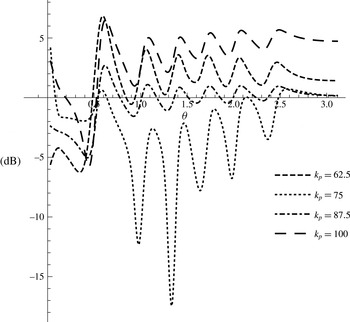
Figure 11. Far-field noise difference in dB at each polar angle
 ${\it\theta}$
between the rigid plate,
${\it\theta}$
between the rigid plate,
 $k_{p}=0.01$
and flexible plates, with
$k_{p}=0.01$
and flexible plates, with
 $M=1.9$
,
$M=1.9$
,
 $L=0.1$
and
$L=0.1$
and
 ${\it\alpha}_{h}=0.0014$
, for
${\it\alpha}_{h}=0.0014$
, for
 $k_{0}=10$
.
$k_{0}=10$
.

Figure 12. Far-field pressure directivity obtained by five monopoles with different locations and frequencies. In all cases
 ${\it\alpha}_{h}=0.0014$
.
${\it\alpha}_{h}=0.0014$
.

Figure 13. Far-field pressure directivity for two different single monopole sources, with
 ${\it\alpha}_{h}=0.0014$
. Results are normalised by the incident pressure amplitude. (a)
${\it\alpha}_{h}=0.0014$
. Results are normalised by the incident pressure amplitude. (a)
 $k_{0}=7.5$
, located at
$k_{0}=7.5$
, located at
 $(0.12,0.02)$
, (b)
$(0.12,0.02)$
, (b)
 $k_{0}=8$
, located at
$k_{0}=8$
, located at
 $(0.145,0.05)$
.
$(0.145,0.05)$
.
We see from figure 10 that by choosing a length and bending wavenumber close to a resonance, a large noise decrease could be achieved. Figure 11 illustrates a similar situation as figure 10 but for
 $k_{0}=10$
and
$k_{0}=10$
and
 $L=0.1$
. We choose different bending wavenumbers to provide consistent bending Mach numbers,
$L=0.1$
. We choose different bending wavenumbers to provide consistent bending Mach numbers,
 ${\it\Omega}=k_{0}/k_{b}$
, as the previous situations, since the bending Mach number was found to be a key parameter in Cavalieri et al. (Reference Cavalieri, Wolf and Jaworski2014). By comparing figures 10 and 11 we see that the same poroelastic plate would have different noise reduction capabilities for different source frequencies. The reduction in noise for
${\it\Omega}=k_{0}/k_{b}$
, as the previous situations, since the bending Mach number was found to be a key parameter in Cavalieri et al. (Reference Cavalieri, Wolf and Jaworski2014). By comparing figures 10 and 11 we see that the same poroelastic plate would have different noise reduction capabilities for different source frequencies. The reduction in noise for
 $k_{p}=75$
occurs due to the proximity of the resonant mode (
$k_{p}=75$
occurs due to the proximity of the resonant mode (
 $0.1\times 75=7.5$
).
$0.1\times 75=7.5$
).
A turbulent boundary layer would contain a vast number of sources at different locations with different frequencies. The results in this paper can allow multiple sources to be assessed. To illustrate this, we consider figure 12 which shows the magnitude of the far-field acoustic pressure produced by five monopoles of equal strength, located at points
 $(0.15,0.06)$
,
$(0.15,0.06)$
,
 $(0.13,0.04)$
,
$(0.13,0.04)$
,
 $(0.14,0.03)$
,
$(0.14,0.03)$
,
 $(0.12,0.02)$
,
$(0.12,0.02)$
,
 $(0.145,0.05)$
, with frequencies
$(0.145,0.05)$
, with frequencies
 $6,6.5,7,7.5,8$
, for a plate with
$6,6.5,7,7.5,8$
, for a plate with
 $L=0.15,M=1.85$
and constant porosity
$L=0.15,M=1.85$
and constant porosity
 ${\it\alpha}_{h}=0.0014$
. Figure 13 shows two of the contributions to figure 12. In figure 13(a) we see a result where the overall sound pressure is decreased for the given flexible plates compared to the rigid plate, whereas in figure 13(b) this is not the case and we see increases in noise for certain values of
${\it\alpha}_{h}=0.0014$
. Figure 13 shows two of the contributions to figure 12. In figure 13(a) we see a result where the overall sound pressure is decreased for the given flexible plates compared to the rigid plate, whereas in figure 13(b) this is not the case and we see increases in noise for certain values of
 $k_{p}$
versus the rigid plate, in particular
$k_{p}$
versus the rigid plate, in particular
 $k_{p}=40,50$
. It is these values of
$k_{p}=40,50$
. It is these values of
 $k_{p}$
that cause an increase in pressure at certain angles in figure 12 which could result in an increase of total scattered noise. We notice however that the increases in figure 12 for the combined five monopoles are much less than the increases seen in the single monopole result in figure 13(b), indicating that over a number of different turbulent sources the capability of the poroelastic plate to increase total noise is lessened.
$k_{p}$
that cause an increase in pressure at certain angles in figure 12 which could result in an increase of total scattered noise. We notice however that the increases in figure 12 for the combined five monopoles are much less than the increases seen in the single monopole result in figure 13(b), indicating that over a number of different turbulent sources the capability of the poroelastic plate to increase total noise is lessened.
By comparing figures 13(a,b) we see that the magnitude of the far-field acoustic directivity for the rigid plates is very different despite the similar sources, indicating that in the case of figure 13(b) there is a strong destructive interference between the leading- and trailing-edge acoustic fields, whereas in figure 13(a) there is not. This explains why, for the same values of
 $k_{p}$
, we do not always see a consistent increase or decrease of noise even though the length of the poroelastic section is the same. The destructive leading- and trailing-edge acoustic interference is dependent on the acoustic source, which differs between figures 13(a,b).
$k_{p}$
, we do not always see a consistent increase or decrease of noise even though the length of the poroelastic section is the same. The destructive leading- and trailing-edge acoustic interference is dependent on the acoustic source, which differs between figures 13(a,b).
6 Conclusions
In this paper we have considered the scattering of acoustic sources by finite rigid plates with finite poroelastic extensions in an attempt to model the noise control properties of the trailing edge of an owl’s wing. Whilst the formulation holds for an arbitrary acoustic source, we have focussed on results in two important cases; far-field sound waves, applicable to rotor blockage within aeroengines, and near-field monopoles, applicable to turbulent boundary layer self-noise. In both cases the rigid section of the plate was seen to be important in determining the potential noise reduction due to interference between acoustic leading- and trailing-edge fields, something that studies for purely poroelastic plates or semi-infinite plates have not assessed. Additionally the length of the poroelastic section was a key parameter affecting noise levels since longer extensions permit more possible resonant modes. We have also presented an approximation method for Wiener–Hopf factorisations, based on Padé approximations. This is particularly effective for this problem since we are concerned only with the far-field scattered acoustics; the method would not be appropriate for calculating the acoustics in the mid or near field.
Blade geometry and mean flow have been excluded from the analysis. An inclusion of either would significantly complicate the modelling of the fluid–structure interaction, and progress with the Wiener–Hopf technique would be difficult. Abrahams (Reference Abrahams1983) discusses the scattering of sound by a finite elastic plate in uniform subsonic flow, however to solve this problem one must use a matched asymptotic expansion in conjunction with the Wiener–Hopf technique. By including a mean flow the sound generated by non-acoustic sources, such as a convective gust from far upstream, could be assessed. Also we have neglected any viscous fluid action within the perforates of the extension. The poroelastic plate model used here presents just a first-order correction to account for the porosity of the plate, provided
 $k_{p}R\ll 1,k_{0}R\ll 1$
and
$k_{p}R\ll 1,k_{0}R\ll 1$
and
 ${\it\alpha}_{h}^{2}\ll 1$
. These restrictions, along with the effects of mean flow on a perforated plate are discussed in Howe (Reference Howe1998). We would anticipate that any effective increase in surface damping (such as including the effects of viscosity within the perforate) could further decrease the far-field scattered sound by decreasing the trailing-edge scattered field, however the interaction between the leading- and trailing-edge fields could still result in noise increases.
${\it\alpha}_{h}^{2}\ll 1$
. These restrictions, along with the effects of mean flow on a perforated plate are discussed in Howe (Reference Howe1998). We would anticipate that any effective increase in surface damping (such as including the effects of viscosity within the perforate) could further decrease the far-field scattered sound by decreasing the trailing-edge scattered field, however the interaction between the leading- and trailing-edge fields could still result in noise increases.
The solution in this paper allows us to calculate the scattered field from multiple near-field sources, as would be found in a turbulent boundary layer above a wind turbine blade. Whilst we have seen that not all single monopole source cases result in an overall decrease of far-field noise for flexible plates compared to fully rigid plates, we would expect, given that we know owls fly almost silently despite turbulence generated within the boundary layers above their wings, that when a large number of sources interact with the poroelastic trailing edge, the noise is reduced overall. In this paper, we have seen that single monopole sources can scatter more noise when interacting with plates with certain poroelastic extensions than when interacting with fully rigid plates. However, the combination of multiple monopole sources results in a much reduced increase in the scattered noise in these situations. We expect that if we included far more near-field sources, any poroelastic extension would reduce the total scattered noise compared to that from a fully rigid plate. Further work is required to support this hypothesis, however it is similar to the results observed for sound generation by wavy leading edges; for single turbulent sources, wavy leading edges have been seen to both increase and decrease noise compared to straight leading edges (Mathews & Peake Reference Mathews and Peake2015). However, fully turbulent flow with a large number of sources predicts a consistent noise reduction for all types of wavy leading edge when compared to straight leading edges (Haeri, Kim & Joseph Reference Haeri, Kim and Joseph2015).
We can conclude that, in agreement with previous studies, poroelastic trailing edges could be a significant tool for reducing sound scattering for a range of acoustic sources, however the interaction of the leading- and trailing-edge scattered fields has the capability of increasing the overall far-field scattered noise when compared to a purely rigid plate.
Acknowledgements
The author is very grateful to C. A. Daly and N. Peake for sharing preliminary work on the case of a semi-infinite rigid section (
 $M\rightarrow \infty$
). The author also wishes to thank A. Kisil for many helpful conversations about the Wiener–Hopf method, and is grateful to Sidney Sussex College for providing financial support.
$M\rightarrow \infty$
). The author also wishes to thank A. Kisil for many helpful conversations about the Wiener–Hopf method, and is grateful to Sidney Sussex College for providing financial support.


