2.1 Geometry, parameters and modelling hypotheses

The geometrical configuration investigated in the present paper is sketched in figure 1. We consider a fluid of viscosity $\unicode[STIX]{x1D708}$ and density $\unicode[STIX]{x1D70C}$ discharging through a circular aperture of radius $R_{h}$ in a planar thick plate with thickness $L_{h}$. The domains located upstream and downstream of the hole are supposed large compared to the dimensions of the hole, so that the geometry is characterized by a single dimensionless parameter, the aspect ratio $\unicode[STIX]{x1D6FD}$ defined as

(2.1)$$\begin{eqnarray}\displaystyle \unicode[STIX]{x1D6FD}=\frac{L_{h}}{2R_{h}}. & & \displaystyle\end{eqnarray}$$

The zero-thickness limit case ($\unicode[STIX]{x1D6FD}=0$) is investigated in detail in Fabre et al. (Reference Fabre, Longobardi, Bonnefis and Luchini2019); in the present paper we consider holes with finite thickness in the range $\unicode[STIX]{x1D6FD}\in [0.1-2]$.

Figure 1. Sketch of the flow configuration (not to scale) representing the oscillating flow through a circular hole in a thick plate, with definition of the geometrical parameters, and indication of the global quantities describing the flow.

The pressure difference between the inlet and the outlet domain, namely $\unicode[STIX]{x0394}P=[P_{in}-P_{out}]$, generates a net flow $Q=U_{M}A_{h}$ through the hole, where $A_{h}=\unicode[STIX]{x03C0}R_{h}^{2}$ is the area of the hole and $U_{M}$ is the mean velocity. This mean flow is characterized by a Reynolds number defined as:

(2.2)$$\begin{eqnarray}\displaystyle Re=\frac{2R_{h}U_{M}}{\unicode[STIX]{x1D708}}\equiv \frac{2Q}{\unicode[STIX]{x03C0}R_{h}\unicode[STIX]{x1D708}}. & & \displaystyle\end{eqnarray}$$

As in Fabre et al. (Reference Fabre, Longobardi, Bonnefis and Luchini2019), we will suppose that the Mach number is small, and that the dimensions of the hole are small compared to the acoustic wavelengths (acoustic compactness hypothesis). These hypotheses allow us to assume that the flow is locally incompressible in the region of the hole. An example of matching with an outer acoustic field is presented in appendix A.

2.2 Characterization of the unsteady regime and impedance definition

To characterize the behaviour of the jet in the unsteady regime, we assume that far away from the hole the pressure levels in the upstream and downstream regions tend to uniform values denoted as $p_{in}(t)$ and $p_{out}(t)$. We will further assume that both the pressure drop $\unicode[STIX]{x0394}p(t)$ and the flow rate $q(t)$ are perturbed by small-amplitude deviations from the mean state characterized by a frequency $\unicode[STIX]{x1D714}$ (possibly complex),

(2.3)$$\begin{eqnarray}\displaystyle \left(\begin{array}{@{}c@{}}\unicode[STIX]{x0394}p(t)\\ q(t)\end{array}\right)=\left(\begin{array}{@{}c@{}}[P_{in}-P_{out}]\\ Q\end{array}\right)+\unicode[STIX]{x1D716}\left(\begin{array}{@{}c@{}}[p_{in}^{\prime }-p_{out}^{\prime }]\\ q^{\prime }\end{array}\right)\text{e}^{-\text{i}\unicode[STIX]{x1D714}t}+\text{c.c.}, & & \displaystyle\end{eqnarray}$$

where the amplitude $\unicode[STIX]{x1D716}$ is assumed small. We can now define the hole impedance as

(2.4)$$\begin{eqnarray}\displaystyle Z_{h}(\unicode[STIX]{x1D714})=\frac{[p_{in}^{\prime }-p_{out}^{\prime }]}{q^{\prime }}. & & \displaystyle\end{eqnarray}$$

Note that with the present definition the impedance has physical units $\text{kg}\cdot \text{s}^{-1}~\text{m}^{-4}$. We will also introduce a non-dimensional impedance defined as

(2.5)$$\begin{eqnarray}\displaystyle Z=\frac{R_{h}^{2}}{\unicode[STIX]{x1D70C}U_{M}}Z_{h}\equiv Z_{R}+iZ_{I}, & & \displaystyle\end{eqnarray}$$

where the real part $Z_{R}$ is the dimensionless resistance while its imaginary part $Z_{I}$ is the reactance. In the presentation of the results, the frequency will be represented in a non-dimensional way by introducing the Strouhal number $\unicode[STIX]{x1D6FA}$ as follows:

(2.6)$$\begin{eqnarray}\displaystyle \unicode[STIX]{x1D6FA}=\frac{\unicode[STIX]{x1D714}R_{h}}{U_{M}}. & & \displaystyle\end{eqnarray}$$

2.3 Impedance-based instability criteria

We now explain the links between impedance and instabilities, and show how simple instability criteria can be formulated using Nyquist diagrams (namely representations of $Z_{r}$ versus $Z_{i}$).

1. (i) First, the sign of the real part of the impedance $Z_{R}(\unicode[STIX]{x1D714})$ (or resistance) as function of the real frequency $\unicode[STIX]{x1D714}$ is a direct indicator of a possible instability. However, one should insist that the condition $Z_{R}<0$ is a necessary but not sufficient condition for instability. In the context of electrical circuits (Conciauro & Puglisi Reference Conciauro and Puglisi1981), a system with negative resistance is said to be active in the sense that it effectively leads to an instability if connected to a reactive circuit allowing oscillations in the right range of frequencies. In the present context, this situation is referred as conditional instability and requires the presence of a correctly tuned acoustic oscillator (a cavity and/or a pipe) connected upstream (or downstream) of the aperture.

   The demonstration that $Z_{R}<0$ is a necessary condition for conditional instability can be explicated in two ways. First, $Z_{R}$ is directly linked to the energy flux transferred from acoustic waves to the jet. The demonstration of this property can be found in Howe (Reference Howe1979), and is also reproduced in Fabre et al. (Reference Fabre, Longobardi, Bonnefis and Luchini2019). Thus, if $Z_{R}>0$ the jet behaves as an energy sink, while if $Z_{R}<0$ it acts as an energy source. Secondly, one can also establish this link by studying the reflection of acoustic waves onto the hole. This argument is carried out in appendix A, where we conduct an asymptotic matching between the locally incompressible solution in the vicinity of the hole and an outer solution of the acoustic problem. The conclusion of this analysis is that, in the limit of small Mach number, an incident acoustic wave coming from the upstream domain is over-reflected if and only if $Z_{R}<0$.

   A situation leading to conditional instability is illustrated in figure 2(a,b). Panel (a) shows the real and imaginary parts of the impedance in a situation where $Z_{R}$ is negative in an interval $[\unicode[STIX]{x1D714}_{1},\unicode[STIX]{x1D714}_{2}]$, and $Z_{i}$ does not change sign. When represented in a Nyquist diagram, the criterion can be formulated as follows: the system is conditionally unstable if the Nyquist curves enter the half-plane $Z_{R}<0$.

2. (ii) Second, when considered as an analytical function of the complex frequency $\unicode[STIX]{x1D714}=\unicode[STIX]{x1D714}_{r}+\text{i}\unicode[STIX]{x1D714}_{i}$, the impedance can be used to formulate a second instability criterion, namely: the system is unstable, regardless of the properties of its environment, if there exists a complex zero of the impedance function such that $\unicode[STIX]{x1D714}_{i}>0$. Indeed, for complex values of $\unicode[STIX]{x1D714}$ the modal dependence reads $\text{e}^{-\text{i}\unicode[STIX]{x1D714}t}=\text{e}^{-\text{i}\unicode[STIX]{x1D714}_{r}t}\text{e}^{\unicode[STIX]{x1D714}_{i}t}$, thus solutions with the form (2.3) are exponentially growing if $\unicode[STIX]{x1D714}_{i}>0$. In the context of electrical circuits, this situation is referred to as absolute instability in opposition to the conditional instability discussed above. Since the term ‘absolute’ has a different meaning in the hydrodynamic stability community (as opposed to convective instabilities, see e.g. Huerre & Monkewitz (Reference Huerre and Monkewitz1990)), we prefer to adopt the term purely hydrodynamic instabilities to describe this case, emphasizing the fact that they can occur in a strictly incompressible framework.

   

   Figure 2. Illustration of the Nyquist-based instability criteria. (a,b) Example of situations leading to conditional instability. (c,d) Example of situations leading to hydrodynamic instability. The regions of conditional and hydrodynamic instabilities are represented by yellow and orange areas, respectively. Left: plot of $Z_{R}$ (solid line) and $Z_{I}$ (dashed line) as a function of the real frequency $\unicode[STIX]{x1D714}$. Right: Nyquist diagrams.

   Physically, the condition $Z_{h}(\unicode[STIX]{x1D714})=0$ implies that there exist modal solutions of the linearized problem in which pressure jump $[p_{in}^{\prime }-p_{out}^{\prime }]$ is exactly zero. In other terms, the total pressure jump across the hole is imposed as a constant (i.e. $[p_{in}(t)-p_{out}(t)]=[P_{in}-P_{out}]$) but the flow rate $q(t)$ is allowed to vary. This kind of boundary condition is a bit uncommon for incompressible flow problems. However, one must keep in mind that the incompressible solution is only valid locally in the vicinity of the hole. In appendix A, we conduct an asymptotic matching with an outer acoustic solution and show that, in the limit of small Mach number, the condition $Z_{h}(\unicode[STIX]{x1D714})=0$ with complex $\unicode[STIX]{x1D714}$ and $\unicode[STIX]{x1D714}_{i}>0$ corresponds to a spontaneous self-oscillation of the flow across the hole associated with the radiation of acoustic waves in both the upstream and downstream domains.

   In practice, the number of complex zeros of the analytically continued impedance $Z_{h}(\unicode[STIX]{x1D714})$ and their location in the complex plane can be deduced from the representation of $Z_{h}(\unicode[STIX]{x1D714})$ for real values $\unicode[STIX]{x1D714}$ using the classical Nyquist criterion, which states that there exists an unstable zero of the impedance if and only if the Nyquist curve encircles the origin in the anticlockwise direction. A weaker but practically equivalent version of this criterion can be formulated as follows: the system is unstable in a purely hydrodynamic way if the Nyquist curve enters the quarter-plane defined by $Z_{R}<0$; $Z_{I}>0$. We refer the reader to Kopitz & Polifke (Reference Kopitz and Polifke2008) for the theoretical background on the use of Nyquist criteria in acoustic applications. Note that the second ‘weak’ form of the criterion used here is not rigorous as it may happen that the Nyquist contour enters the quarter-plane and leaves it by the same side without encircling the origin, in which case the criterion would erroneously predict instability. We carefully checked that such behaviour does not occur in the computed cases. (A situation leading to purely hydrodynamic instability is illustrated in figure 2(c,d).)

   In addition to providing an instability criterion, the knowledge of the impedance for real $\unicode[STIX]{x1D714}$ can also be used to predict an approximation of the complex zeros in the case where $\unicode[STIX]{x1D714}_{i}$ is small. For this sake, let us suppose that the Nyquist curve passes close to the origin, and let us denote $\unicode[STIX]{x1D714}_{0}$ the value for which the norm of the complex impedance $|Z(\unicode[STIX]{x1D714})|$ is smallest. The location of this point is illustrated in figure 2(c,d). Searching for the complex zero as $\unicode[STIX]{x1D714}=\unicode[STIX]{x1D714}_{0}+\unicode[STIX]{x1D6FF}\unicode[STIX]{x1D714}$ and working with a Taylor series around $\unicode[STIX]{x1D714}_{0}$ leads to

   (2.7)$$\begin{eqnarray}\displaystyle Z(\unicode[STIX]{x1D714}_{0})+(\unicode[STIX]{x2202}Z/\unicode[STIX]{x2202}\unicode[STIX]{x1D714})_{\unicode[STIX]{x1D714}_{0}}\unicode[STIX]{x1D6FF}\unicode[STIX]{x1D714}=0, & & \displaystyle\end{eqnarray}$$
   hence providing an estimation as follows:
   (2.8)$$\begin{eqnarray}\displaystyle \unicode[STIX]{x1D714}\approx \unicode[STIX]{x1D714}_{0}-\frac{Z(\unicode[STIX]{x1D714}_{0})\overline{(\unicode[STIX]{x2202}Z/\unicode[STIX]{x2202}\unicode[STIX]{x1D714})}_{\unicode[STIX]{x1D714}_{0}}}{|(\unicode[STIX]{x2202}Z/\unicode[STIX]{x2202}\unicode[STIX]{x1D714})_{\unicode[STIX]{x1D714}_{0}}|^{2}}. & & \displaystyle\end{eqnarray}$$
   It can be shown that $Z(\unicode[STIX]{x1D714}_{0})\overline{(\unicode[STIX]{x2202}Z/\unicode[STIX]{x2202}\unicode[STIX]{x1D714})}_{\unicode[STIX]{x1D714}_{0}}$ is purely imaginary (a simple geometrical interpretation being that the line joining the point $Z(\unicode[STIX]{x1D714}_{0})$ to the origin and the line tangent to the Nyquist curve at $\unicode[STIX]{x1D714}_{0}$ are orthogonal to each other). Hence, the correction appearing in (2.8) directly provides an estimation of the amplification rate $\unicode[STIX]{x1D714}_{i}$.

3.1 Starting equations

The fluid motion is governed by the Navier–Stokes equations,

(3.1)$$\begin{eqnarray}\displaystyle \frac{\unicode[STIX]{x2202}}{\unicode[STIX]{x2202}t}\left[\begin{array}{@{}c@{}}\boldsymbol{u}\\ 0\end{array}\right]={\mathcal{N}}{\mathcal{S}}\left(\left[\begin{array}{@{}c@{}}\boldsymbol{u}\\ p\end{array}\right]\right)=\left[\begin{array}{@{}c@{}}-\boldsymbol{u}\boldsymbol{\cdot }\unicode[STIX]{x1D735}\boldsymbol{u}-\unicode[STIX]{x1D735}p+Re^{-1}\unicode[STIX]{x1D6FB}^{2}\boldsymbol{u}\\ \unicode[STIX]{x1D735}\boldsymbol{\cdot }\boldsymbol{u}\end{array}\right], & & \displaystyle\end{eqnarray}$$

where $\boldsymbol{u}$ and $p$ are the velocity and pressure fields.

The linearized Navier–Stokes framework consists of expanding the flow as a steady base flow plus a small-amplitude modal perturbation as follows:

(3.2)$$\begin{eqnarray}\displaystyle \left[\begin{array}{@{}c@{}}\boldsymbol{u}\\ p\end{array}\right]=\left[\begin{array}{@{}c@{}}\boldsymbol{u}_{\mathbf{0}}\\ p_{0}\end{array}\right]+\unicode[STIX]{x1D716}\left(\left[\begin{array}{@{}c@{}}\boldsymbol{u}^{\prime }\\ p^{\prime }\end{array}\right]\text{e}^{-\text{i}\unicode[STIX]{x1D714}t}+\text{c.c.}\right), & & \displaystyle\end{eqnarray}$$

where c.c. denotes the complex conjugate.

Figure 3. Structure of the mesh $\mathbb{M}_{1}$ obtained using complex mapping and mesh adaptation for $\unicode[STIX]{x1D6FD}=1$, and nomenclature of the boundaries (see appendix B for details on mesh generation and validation). A zoom of the mesh is reported in the range $X\in [-2.5;0.5]R_{h}$ and $R\in [0.1;1.8]R_{h}$.

In practice, the base flow $[\boldsymbol{u}_{\mathbf{0}},p_{0}]$ and perturbation $[\boldsymbol{u}^{\prime },p^{\prime }]$ will be computed in a computational domain of finite size with boundaries denoted $\unicode[STIX]{x1D6E4}_{in},\unicode[STIX]{x1D6E4}_{out},\unicode[STIX]{x1D6E4}_{wall},\unicode[STIX]{x1D6E4}_{lat},\unicode[STIX]{x1D6E4}_{axis}$ (see figure 3). The matching with the global quantities $P_{in},P_{out}$ etc. will be done through the boundary conditions on $\unicode[STIX]{x1D6E4}_{in}$ and $\unicode[STIX]{x1D6E4}_{out}$. This matching procedure involves a number of caveats, which were discussed at length in Fabre et al. (Reference Fabre, Longobardi, Bonnefis and Luchini2019). We refer to this work for full details, but restrict ourselves in this paragraph to a simple exposition of the procedure.

3.2 Base-flow equations

The base flow is the solution of the steady version of the Navier–Stokes equations,

(3.3)$$\begin{eqnarray}\displaystyle {\mathcal{N}}{\mathcal{S}}[\boldsymbol{u}_{\mathbf{0}};p_{0}]=0, & & \displaystyle\end{eqnarray}$$

with the following set of boundary conditions:

(3.4)$$\begin{eqnarray}\displaystyle & \displaystyle \int _{\unicode[STIX]{x1D6E4}_{in}}\boldsymbol{u}_{\mathbf{0}}\boldsymbol{\cdot }\boldsymbol{n}\,\text{d}S=Q_{0} & \displaystyle\end{eqnarray}$$

(3.5)$$\begin{eqnarray}\displaystyle & \displaystyle p_{0}=P_{in}\quad \text{on}~\unicode[STIX]{x1D6E4}_{in}, & \displaystyle\end{eqnarray}$$

(3.6)$$\begin{eqnarray}\displaystyle & \displaystyle p_{0}=P_{out}\quad \text{on}~\unicode[STIX]{x1D6E4}_{out}. & \displaystyle\end{eqnarray}$$

In practice, (3.4) is enforced as a Dirichlet boundary condition by prescribing a constant value of the axial velocity component, i.e. $u_{0,x}=Q_{0}/(\int _{\unicode[STIX]{x1D6E4}_{in}}\,\text{d}S)$. Noting that the pressure reference can be arbitrarily chosen such that $P_{out}=0$ and that the viscous stress is negligible along the outlet plane, (3.6) is enforced as a no-stress condition. This problem is solved iteratively using Newton’s method, exactly as done in Fabre et al. (Reference Fabre, Citro, Sabino, Bonnefis, Sierra, Giannetti and Pigou2018). Eventually, (3.5) is used to extract $P_{in}$ as the average value of $p_{0}$ along the inlet plane, allowing us to deduce the discharge coefficient $\unicode[STIX]{x1D6FC}$ (see § 4).

3.3 Linear equations

The linear perturbation obeys the following equations:

(3.7)$$\begin{eqnarray}\displaystyle -\text{i}\unicode[STIX]{x1D714}{\mathcal{B}}[\boldsymbol{u}^{\prime };p^{\prime }]={\mathcal{L}}{\mathcal{N}}{\mathcal{S}}_{0}[\boldsymbol{u}^{\prime };p^{\prime }], & & \displaystyle\end{eqnarray}$$

where ${\mathcal{L}}{\mathcal{N}}{\mathcal{S}}_{0}$ is the linearized Navier–Stokes operator around the base flow and ${\mathcal{B}}$ is a weight operator defined as follows:

(3.8a,b)$$\begin{eqnarray}\displaystyle {\mathcal{L}}{\mathcal{N}}{\mathcal{S}}_{0}\left[\begin{array}{@{}c@{}}\boldsymbol{u}^{\prime }\\ p^{\prime }\end{array}\right]=\left[\begin{array}{@{}c@{}}-(\boldsymbol{u}_{0}\boldsymbol{\cdot }\unicode[STIX]{x1D735}\boldsymbol{u}^{\prime }+\boldsymbol{u}^{\prime }\boldsymbol{\cdot }\unicode[STIX]{x1D735}\boldsymbol{u}_{0})-\unicode[STIX]{x1D735}p^{\prime }+Re^{-1}\unicode[STIX]{x1D6FB}^{2}\boldsymbol{u}^{\prime }\\ \unicode[STIX]{x1D735}\boldsymbol{\cdot }\boldsymbol{u}^{\prime }\end{array}\right];\quad {\mathcal{B}}=\left[\begin{array}{@{}cc@{}}1 & 0\\ 0 & 0\end{array}\right].\qquad & & \displaystyle\end{eqnarray}$$

This set of equations is complemented by the following boundary conditions:

(3.9)$$\begin{eqnarray}\displaystyle & \displaystyle \int _{\unicode[STIX]{x1D6E4}_{in}}\boldsymbol{u}^{\prime }\boldsymbol{\cdot }\boldsymbol{n}\,\text{d}S=q^{\prime }, & \displaystyle\end{eqnarray}$$

(3.10)$$\begin{eqnarray}\displaystyle & \displaystyle p^{\prime }(x,r)=p_{in}^{\prime }\quad \text{on }\unicode[STIX]{x1D6E4}_{in}, & \displaystyle\end{eqnarray}$$

(3.11)$$\begin{eqnarray}\displaystyle & \displaystyle p^{\prime }(x,r)=p_{out}^{\prime }\quad \text{on }\unicode[STIX]{x1D6E4}_{out}. & \displaystyle\end{eqnarray}$$

This system governs the evolution of the perturbations and is relevant to both the forced problem and the autonomous problem. The difference is in the possible dependence with respect to the azimuthal coordinate $\unicode[STIX]{x1D703}$ and in the handling of the boundary conditions:

1. (i) For the forced problem, the forcing being axisymmetric, the perturbation is expected to respect this symmetry and is thus searched under the form $[\boldsymbol{u}^{\prime };p^{\prime }]=[u_{r}^{\prime }(r,z),u_{x}^{\prime }(r,z),;p^{\prime }(r,z)]$. Furthermore, a non-zero $q^{\prime }$ is imposed (fixed arbitrarily to $q^{\prime }=1$). Equation (3.9) thus leads to a non-homogeneous Dirichlet boundary condition at the inlet plane treated by imposing a constant axial velocity $u_{x}^{\prime }$. For the same reasons as for the base-flow equations,  (3.11) can be replaced by a no-stress boundary condition on $\unicode[STIX]{x1D6E4}_{out}$. The problem can be symbolically written as

   (3.12)$$\begin{eqnarray}\displaystyle [{\mathcal{L}}{\mathcal{N}}{\mathcal{S}}_{0}-\text{i}\unicode[STIX]{x1D714}{\mathcal{B}}][\boldsymbol{u}^{\prime };p^{\prime }]={\mathcal{F}}, & & \displaystyle\end{eqnarray}$$
   where the definition of ${\mathcal{L}}{\mathcal{N}}{\mathcal{S}}_{0}$ implicitly contains the homogeneous boundary condition at the outlet, and ${\mathcal{F}}$ represents symbolically the non-homogeneous boundary condition at the inlet. This problem is non-singular and readily solved. The pressure $p_{in}^{\prime }$ is subsequently deduced from (3.10) by extracting the mean value of the $p^{\prime }$ component along the inlet boundary $\unicode[STIX]{x1D6E4}_{in}$ of the computational domain, eventually allowing us to compute the impedance.

2. (ii) For the homogeneous problem, on the other hand, there is no a priori reason to assume axisymmetry, hence the perturbation may be assumed to have azimuthal dependence with a wavenumber $m$, namely $[\boldsymbol{u}^{\prime },p^{\prime }]=[\hat{\boldsymbol{u}},\hat{p}]\text{e}^{\text{i}m\unicode[STIX]{x1D703}}$. For axisymmetric modes ($m=0$), as discussed in § 2 and appendix A, the relevant boundary conditions arising from a matching with an outer acoustic solution are $\hat{p}_{in}=\hat{p}_{out}=0$, which can be practically enforced as no-stress conditions at both the inlet and the outlet. When looking for non-axisymmetric modes ($m\neq 0$), on the other hand, it makes more sense to impose $u_{x}^{\prime }=0$ on the inlet (as there is no net flux $q^{\prime }$ through the hole in such cases) and no stress at the outlet. The problem can be symbolically written in the form

   (3.13)$$\begin{eqnarray}\displaystyle [{\mathcal{L}}{\mathcal{N}}{\mathcal{S}}_{0}^{\ast }-\text{i}\unicode[STIX]{x1D714}{\mathcal{B}}][\hat{\boldsymbol{u}};\hat{p}]=0, & & \displaystyle\end{eqnarray}$$
   where the operator ${\mathcal{L}}{\mathcal{N}}{\mathcal{S}}_{0}^{\ast }$ implicitly contains the homogeneous conditions at both upstream and downstream boundaries. For $m=0$, the flow rate $\hat{q}$ associated with the eigenmodes through (3.9) is generally non-zero, so the eigenmodes can be rescaled such that $\hat{q}=1$.

   After discretization of the operators ${\mathcal{L}}{\mathcal{N}}{\mathcal{S}}_{0}^{\ast }$ and ${\mathcal{B}}$ as large matrices, we are led to a generalized eigenvalue problem, which admits a discrete set of complex eigenvalues $\unicode[STIX]{x1D714}=\unicode[STIX]{x1D714}_{r}+\text{i}\unicode[STIX]{x1D714}_{i}$. As usual in stability analysis of open flows, only a small number of these eigenvalues correspond to physically relevant global eigenmodes. The remainder, often referred to as ‘artificial modes’, include both a discretized version of the continuous spectrum and spurious modes induced by the truncation of the domain to a finite size (Lesshafft Reference Lesshafft2018). Appendix B details how to sort ‘physical modes’ from ‘artificial modes’ and details the effect of the complex mapping technique used here on the latter set of modes.

Aside from the determinations of the (direct) eigenmodes $[\hat{\boldsymbol{u}},\hat{p}]$, it is also useful to study the structure of the adjoint eigenmodes $[\hat{\boldsymbol{u}}^{\dagger },\hat{p}^{\dagger }]$, namely the eigenmodes of the adjoint operator ${\mathcal{L}}{\mathcal{N}}{\mathcal{S}}_{0}^{\ast \dagger }$. We refer to Luchini & Bottaro (Reference Luchini and Bottaro2014) for a detailed discussion of the topic. In the present paper we adopt a discrete adjoint approach.

The structural sensitivity (Giannetti & Luchini Reference Giannetti and Luchini2007) of a hydrodynamic oscillator is also used in the present manuscript to identify the flow region where the mechanism of instability acts. In particular, we follow Giannetti & Luchini (Reference Giannetti and Luchini2007) to build a spatial sensitivity map by computing the spectral norm of the sensitivity tensor:

(3.14)$$\begin{eqnarray}\displaystyle \unicode[STIX]{x1D64E}(x,r)=\frac{\hat{\boldsymbol{u}}^{\dagger }(x,r)\otimes \hat{\boldsymbol{u}}(x,r)}{\displaystyle \int _{D}\hat{\boldsymbol{u}}^{\dagger }(x,r)\hat{\boldsymbol{u}}(x,r)\,\text{d}D}, & & \displaystyle\end{eqnarray}$$

where $D$ is the computational domain.

3.4 Numerical method

The results presented here are obtained with the same numerical method as used in Fabre et al. (Reference Fabre, Longobardi, Bonnefis and Luchini2019). The mesh construction and adaptation, computation of the base flow and of the linear problems are implemented using the open-source finite element software FreeFem++. The main originalities of the present implementation are the use of complex mapping in the axial direction to overcome problems associated with the large convective amplification of structures in the downstream direction (see Fabre et al. Reference Fabre, Longobardi, Bonnefis and Luchini2019), and the systematic use of mesh adaptation to substantially reduce the required number of degrees of freedom (following a methodology described in Fabre et al. (Reference Fabre, Citro, Sabino, Bonnefis, Sierra, Giannetti and Pigou2018) and previously used for the zero-thickness hole in Fabre et al. (Reference Fabre, Longobardi, Bonnefis and Luchini2019)). An example of an unstructured grid obtained in this way is displayed in figure 3. Note that the downstream dimension $L_{out}$ in numerical coordinates seems rather short; however, as the coordinate mapping used in this case involves a stretching, the actual dimension in physical coordinates is much larger.

The loops over parameters and generation of the figures are performed using Octave/Matlab thanks to the generic drivers of the StabFem project (see a presentation of these functionalities in Fabre et al. (Reference Fabre, Citro, Sabino, Bonnefis, Sierra, Giannetti and Pigou2018)). According to the philosophy of this project, all the codes used in the present paper are available from the StabFem website (gitlab.com/stabfem/StabFem), and a simple script reproducing the main results of the present paper is provided (gitlab.com/stabfem/StabFem/STABLE_CASES/WHISTLE/SCRIPT_chi1.m.). On a standard laptop, all the computations discussed below can be obtained in a few hours. Numerical convergence issues are discussed in appendix B by comparing results obtained with four different meshes, with variable domain dimension and grid density (controlled by using several mesh adaptation strategies).

5.1 Case $\unicode[STIX]{x1D6FD}=0.3$

As previously introduced, the most important quantity associated with the unsteady flow is the impedance $Z=Z_{R}+iZ_{I}$. This quantity is plotted as function of the frequency in figure 7 for Reynolds numbers ranging from $800$ to $2000$. The plots in the left column display $Z_{R}$ and $Z_{I}$ as functions of $\unicode[STIX]{x1D6FA}$ (note that as $Z_{I}$ is generally negative and decreasing with $\unicode[STIX]{x1D6FA}$, it is convenient to plot $-Z_{I}/\unicode[STIX]{x1D6FA}$). The right column displays the corresponding Nyquist diagrams.

Figure 7. Impedance of the flow through a circular aperture with aspect ratio $\unicode[STIX]{x1D6FD}=0.3$. (a,c,e,g) Plot of $Z_{R}$ (solid line) and $Z_{I}$ (dashed line) as a function of the perturbation frequency $\unicode[STIX]{x1D6FA}$; (b,d,f,h) Nyquist diagrams for (a,b), $Re=800$, (c,d), $Re=1200$, (e,f), $Re=1600$, (g,h), $Re=2000$. Points (C1), (S1) and (C2) indicate the locations corresponding to the structures shown in figures 8 and 9. Point ‘O’ indicates the starting point ($\unicode[STIX]{x1D6FA}=0$) of the Nyquist curves.

For $Re=800$ (a,b), the system presents a small frequency interval near $\unicode[STIX]{x1D6FA}\approx 2.2$ with negative values of the real part of the impedance $Z_{R}$. As explained in § 2.3, this property is directly related to a possible instability. On the other hand, the imaginary part $Z_{I}$ is always negative in the range of frequencies considered.

As the Reynolds number is increased further, one observes that the region of negative $Z_{R}$ gets larger and reaches larger values. Note also that the negative, minimum value of $Z_{R}$ is associated with a maximum of $-Z_{I}/\unicode[STIX]{x1D6FA}$. Increasing the Reynolds number enlarges the range of $\unicode[STIX]{x1D714}$ where the system has negative values of $Z_{R}$. The cases (e,g) associated with $Re=1600,2000$ show a second region of conditional instability for higher frequencies in the range near $\unicode[STIX]{x1D6FA}\approx 8.5$. This is again associated with a maximum of $-Z_{I}/\unicode[STIX]{x1D6FA}$. Note that for Reynolds numbers up to $2000$ we do not find a hydrodynamic instability. We recall that the number of unstable modes (absolute instability) is associated with the number of times the contour of the complex impedance $Z_{h}$ encircles the origin. This condition is never satisfied in figure 7.

Figure 8. Structure of the unsteady flow for $\unicode[STIX]{x1D6FD}=0.3$ and $Re=1600$. (a,c,e) Real part of the pressure component; (b,d,f) imaginary part of the pressure component. First row (C1): $\unicode[STIX]{x1D6FA}=2.6$ (conditionally unstable case with $Z_{r}<0$); second row (S1) $\unicode[STIX]{x1D6FA}=5.45$ (stable case with $Z_{r}>0$); third row (C2) $\unicode[STIX]{x1D6FA}=8.25$ (conditionally unstable case with $Z_{r}<0$).

To explain these trends, and in particular the possibility of negative $Z_{R}$, we now depict in figure 8 the structure of the flow perturbation for three values of the frequency, corresponding to points C1, S1 and C2, as indicated in figure 7(f). The cases C1 and C2 correspond to the two first negative minima of $Z_{R}$, hence to conditionally unstable cases, while case S1 corresponds to a positive maximum of $Z_{R}(\unicode[STIX]{x1D6FA})$, hence to a maximally stable case. The plot shows the real and imaginary part of the pressure component $p^{\prime }$, which correspond respectively to the components in phase with the oscillating flow rate and a quarter period after (at the instant when the oscillating flow reverses). The figure shows that the harmonic forcing generates alternating high and low pressure regions which propagate along the shear layer and are amplified downstream. Note that the plots use a logarithmically stretched colour scale, allowing us to visualize the structure despite the very strong spatial amplification.

Thanks to the normalization of the oscillating flow by $q^{\prime }=1$ and the pressure reference taken as $p_{out}^{\prime }=0$, the impedance $Z=[p_{in}^{\prime }-p_{out}^{\prime }]/q^{\prime }$ can be directly read on the figures from the uniform value of the pressure in the upstream domain. Accordingly, for the conditionally unstable cases, C1 and C2, one can see that the real part of $p_{in}^{\prime }$ is negative, while for the stable case ($c$) it is positive. On the other hand, the imaginary part of $p_{in}^{\prime }$ is negative in the three cases (see the plots in the right column of the figure), consistently with the fact that $Z_{I}$ is always negative for $\unicode[STIX]{x1D6FD}=0.3$.

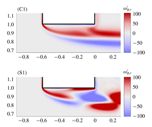
Figure 9. Left: vorticity component $\unicode[STIX]{x1D714}_{r}^{\prime }$ (real part) of the perturbation. Right: reconstruction of the structure of the perturbed shear layer ($\text{base flow}+\text{perturbation}$) at the instant corresponding to maximum flow rate through the hole for $\unicode[STIX]{x1D6FD}=0.3$ and $Re=1600$. Cases (C1), (S1), (C2) as in figure 8.

Figure 9 complements the description of the structure of the perturbation for the same three values of the frequency, by analysing the dynamics of the shear layer. For this we focus on the real part of the vorticity component $\unicode[STIX]{x1D714}_{r}^{\prime }$ corresponding to the instant of the cycle where the flow rate through the hole is maximum. For case (C1) (first row), at this instant the vorticity perturbation consists of two layers of vorticity of opposite sign, with positive sign in the region closest to the hole. When superposing this perturbation onto the base flow, which consists of a shear layer of positive vorticity (see e.g. the lower half of figure 4), the result is to shift the shear layer towards the walls, as schematically represented in the plot on the right. The section of the jet is thus locally enlarged in the outlet section, hence the velocity is reduced, and according to the Bernoulli law the pressure $p_{s}^{\prime }$ at the outlet section (which may be identified with the real part of $p_{out}^{\prime }$) at this location is increased. This simple argument allows us to explain why the fluctuating pressure jump at the considered instant of the cycle $\text{Re}[p_{in}^{\prime }-p_{out}^{\prime }]$ is negative.

For the case C2 with $\unicode[STIX]{x1D6FA}=8.25$ (third row), the structure of the vorticity perturbation is more complex and changes sign twice between the upstream and downstream sides of the holes. Superposing this onto a base flow leads to a situation where the shear layer is first displaced towards the wall, then away from it and again towards it. The simple Bernoulli argument thus leads to the same conclusion, namely an increase of the pressure $p_{s}^{\prime }$ in the outlet plane.

On the other hand, for the stable case (S1) with $\unicode[STIX]{x1D6FA}=5.45$ the structure of the vorticity perturbation changes sign only once. The result is that the shear layer is displaced away from the wall in the outlet plane. The simple Bernoulli argument leads, in this case, to a decrease of the pressure $p_{s}^{\prime }$ in the outlet plane.

The explanation presented here is not fully rigorous, in particular because the impedance is based on the pressure $p_{out}^{\prime }$ far downstream and not the one $p_{s}^{\prime }$ at the outlet of the hole. The validity of the Bernoulli law is also questionable in such unsteady regimes. Eventually, the argument assumes a fully detached shear layer and does not explain why instability is also possible in ranges of Reynolds numbers where the recirculation bubble is closed. Still, we believe this reasoning gives a simple explanation to the fact that minima of $Z_{R}$ (potentially unstable situations) are associated with an odd number of structures within the thickness while maxima of $Z_{R}$ (most stable situations) are associated with an even number of structures within the thickness of the hole.

Figure 10. Impedance results for $\unicode[STIX]{x1D6FD}=1$. (a,c,e,g) Plot of $Z_{R}$ (solid line) and $Z_{I}$ (dashed line) as functions of the perturbation frequency $\unicode[STIX]{x1D6FA}$. (b,d,f,h) Nyquist diagrams for (a,b), $Re=800$, (c,d), $Re=1200$, (e,f), $Re=1600$, (g,h), $Re=2000$. Points (C1), (S1), (H2), (C2) and (S2) indicate the locations corresponding to the structures shown in figures 11 and 12. Point ‘O’ indicates the starting point ($\unicode[STIX]{x1D6FA}=0$) of the Nyquist curves.

5.2 Case $\unicode[STIX]{x1D6FD}=1$

We now consider the case of a thicker hole with aspect ratio $\unicode[STIX]{x1D6FD}=1$. Figure 10 plots the impedance for $Re$ from $800$ to $2000$. As in the previous case detailed in § 5.1, one can see the existence of several frequency intervals where $Z_{R}$ becomes negative.

The real and imaginary parts of the impedance $Z_{h}$ are always positive for $Re=800$ (see figure 10a). As a consequence, the associated Nyquist curve plotted in figure 10(b) does not cross the $Z_{R}=0$ axis. The system displays two intervals of conditional instability at $Re=1200$, around $\unicode[STIX]{x1D6FA}\approx 2.5$ and $\unicode[STIX]{x1D6FA}\approx 4.7$, respectively. Note that the real part $Z_{R}$ presents larger oscillations than in the corresponding case at $\unicode[STIX]{x1D6FD}=0.3$.

When the Reynolds number is increased, both real and imaginary parts of the impedance reach very large values. Figure 10(e) plots $Z_{R}$ and $-Z_{I}/\unicode[STIX]{x1D6FA}$ for $Re=1600$ and reveals four intervals of conditional instability and one interval of hydrodynamic instability. Another important result which can be seen in this figure is the existence of true zeros of the impedance. This happens in particular at $\unicode[STIX]{x1D6FA}\approx 2.07$. This property reveals the existence of a purely hydrodynamic instability, as discussed in § 3. This point will be further confirmed in § 6. Further increasing the Reynolds number to $Re=2000$ produces a second interval of hydrodynamic instability around $\unicode[STIX]{x1D6FA}=4.4$.

Figure 11. Structure of the unsteady flows for $\unicode[STIX]{x1D6FD}=1$ and $Re=2000$. Real (a,c,e) and imaginary (b,d,f) parts of the pressure component: (C1) conditionally unstable case with $\unicode[STIX]{x1D6FA}=0.95$; (S1) stable case with $\unicode[STIX]{x1D6FA}=1.85$; (H2) unconditionally unstable case with $\unicode[STIX]{x1D6FA}=2.5$; (C2) conditionally unstable case with $\unicode[STIX]{x1D6FA}=2.7$; (S2) stable case with $\unicode[STIX]{x1D6FA}=3.8$.

In figures 11 and 12, we represent the pressure and vorticity components of the perturbations for $Re=2000$ for five selected values of $\unicode[STIX]{x1D6FA}$ corresponding to points C1, S1, H2, C2, S2 as indicated in figure 10(h). Cases (C1, C2) and (S1, S2) correspond to minima and maxima of $Z_{R}$, while case (H2) correspond to the first positive maximum of $Z_{I}$.

In the pressure plots (figure 11), the same observations can be made as previously for $\unicode[STIX]{x1D6FD}=0.3$, namely the real part of the pressure in the upstream domain is negative for conditionally unstable cases (C1) and (C2) and positive for stable cases ((S1) and (S2)). The case (H2) (third row) differs from all other cases by one property: the imaginary part of the upstream pressure is positive (see right plot).

Inspecting the real part of the vorticity perturbation (left column in figure 12) allows us to draw the same conclusions as in the previous section, namely conditionally unstable cases display an odd number of structures within the thickness and stable ones display an even number of structures. We may thus conclude that the simple argument explained in the previous paragraph and illustrated in the right column of figure 9 is also valid for $\unicode[STIX]{x1D6FD}=1$.

For the unconditionally unstable case H2, the real part of the vorticity is quite similar to the conditionally unstable case (C2) and allows us to justify that $Z_{R}$ is also negative in this case. On the other hand, inspecting the imaginary part of the vorticity perturbation (plot in the right column) does not easily allow us to justify that $Z_{I}$ is positive for case (H2), unlike all the other cases. It does not seem possible to give a simple explanation of the unconditional instability in terms of oscillations of the shear layer. We assume that the mechanism is more complex and includes some feedback mechanism occurring within the recirculation region.

Figure 12. Structure of the unsteady flows for $\unicode[STIX]{x1D6FD}=1$ and $Re=2000$. Real (a,c,e) and imaginary (b,d,f) parts of the vorticity component, for the same values of $\unicode[STIX]{x1D6FA}$ as in figure 11.

5.3 Parametric study

In the previous sections, we documented the impedance results for $\unicode[STIX]{x1D6FD}=0.3$ and $\unicode[STIX]{x1D6FD}=1$. In both cases, when increasing the Reynolds number, we observed the emergence of an increasing number of intervals of conditional instability, associated with the crossing of the real axis in the Nyquist diagram by successive ‘loops’ of the Nyquist curve. In addition, but only for $\unicode[STIX]{x1D6FD}=1$, we observed the emergence of an increasing number of purely hydrodynamic instabilities associated with the encircling of the origin by successive loops of the same curve. In this section, we present the results of a parametric study which allowed us to identify the regions of the conditional and hydrodynamic instabilities in the range $\unicode[STIX]{x1D6FD}=[0.1-2]$; $Re=[500-2000]$.

Figure 13. Thresholds for the onset of conditional instability (C1 to C4) and of hydrodynamic instability (H2 and H3).

Figure 14. Frequencies corresponding to conditional instability (C1 to C4) and hydrodynamic instability (H2 and H3).

Figure 13 shows the critical Reynolds number associated with each instability branch as a function of the aspect ratio $\unicode[STIX]{x1D6FD}$. In this figure, curves labelled C1 to C4 correspond to the first four branches of the conditional instabilities, while branches H2 and H3 correspond to the first two branches of the hydrodynamic instabilities. We adopted this labelling because these instabilities are associated with the same ‘loops’ in the Nyquist curve as modes C2 and C3. Note that no crossing of the origin was ever observed along the first loop; this is why the figure does not display any H1 branch.

For short holes, branch C1 is the first to become unstable and branches C2, C3 etc. are only encountered at substantially larger $Re$. This is compatible with the results of figure 7 for $\unicode[STIX]{x1D6FD}=0.3$, which indicates that branch C1 becomes unstable slightly below $Re=800$ and branch C2 between 1200 and 1600. The situation is different for longer holes as branches C2, C3 successively become the most unstable ones. For instance, for $\unicode[STIX]{x1D6FD}=1$, conditional instability first happens along branch C2 just above $Re=800$, and, as $Re$ is further increased, branches C3, C4 and C1 are then encountered in this order. This is again fully compatible with the Nyquist diagrams of figure 10.

Hydrodynamic instabilities generally occur at larger Reynolds numbers than conditional instabilities, and are encountered only for sufficiently thick holes ($\unicode[STIX]{x1D6FD}>0.5$). For $\unicode[STIX]{x1D6FD}=1$, branch H2 becomes unstable for $Re\approx 1500$ and branch H3 for $Re\approx 1700$. This is again fully compatible with the Nyquist representations in figure 10.

We finally notice that for $\unicode[STIX]{x1D6FD}<0.1$ no instability is found in the range investigated. This suggests that the limiting case of zero thickness is unconditionally stable, in accordance with the classical model of Howe and our previous investigation of this case (Fabre et al. Reference Fabre, Longobardi, Bonnefis and Luchini2019).

The frequencies associated with each of the instability branches are plotted in figure 14. We start by plotting the Strouhal number based on the hole radius $R_{h}$ as a function of the aspect ratio $\unicode[STIX]{x1D6FD}$. Note that the frequencies associated with hydrodynamic instabilities H2 and H3 closely follow those associated with conditional instabilities C2 and C3, thus confirming our nomenclature choice.

It is interesting to note that all branches indicate that the frequency is inversely proportional to the aspect ratio of the hole. This suggests that, instead of the definition $\unicode[STIX]{x1D6FA}$ used up to now, it may be better to define a Strouhal number based on the thickness of the hole as follows:

(5.1)$$\begin{eqnarray}\displaystyle St_{L}=\frac{f\,L}{U_{M}}\equiv \frac{\unicode[STIX]{x1D6FA}\unicode[STIX]{x1D6FD}}{\unicode[STIX]{x03C0}}. & & \displaystyle\end{eqnarray}$$

Plotting results using this definition leads to figure 14(b), which confirms that the Strouhal number is almost independent of the aspect ratio for all branches.

6.1 Eigenvalues

The stability characteristics of the base flow are assessed by monitoring the evolution of the leading global modes. Figure 15(a) shows the growth rate $\unicode[STIX]{x1D714}_{i}$ for the three least stable modes for $\unicode[STIX]{x1D6FD}=1$. Two of them become unstable in the plotted range of $Re$. The first branch becomes unstable at $Re\approx 1500$ while the second one presents a critical Reynolds number equal to $Re\approx 1700$. This is fully compatible with the impedance predictions corresponding to branches H2 and H3 discussed in the previous section.

Figure 15(b) displays the oscillation rate $\unicode[STIX]{x1D714}_{r}$ for the same three modes. The three branches display an almost constant value of the radius-based Strouhal number $\unicode[STIX]{x1D6FA}$. The values for the unstable modes are $\unicode[STIX]{x1D6FA}\approx 2.1$ and $\unicode[STIX]{x1D6FA}\approx 4.2$, in perfect accordance with the expected values for modes H2 and H3.

Note that figure 15(a,b) displays the existence of a third branch of eigenvalues which is always stable. The corresponding frequency is observed for $\unicode[STIX]{x1D6FA}\approx 0.5$, which corresponds to a value for which the first ‘loop’ of the Nyquist curve comes close to zero, but does not encircle it. This allows us to identify this mode with the ‘H1’ mode which was missing in figure 13. This mode actually exists as a global mode but remains stable for all values of $Re$ and $\unicode[STIX]{x1D6FD}$ in the investigated range.

As discussed in § 2, in addition to providing an instability criterion, knowledge of the impedance for real $\unicode[STIX]{x1D714}$ also provides an estimation of the eigenvalues associated with the purely hydrodynamic instability valid in the case where $\unicode[STIX]{x1D714}_{i}$ is small. To demonstrate this, we have plotted with symbols in figure 15(a) the prediction of the asymptotic formula (2.8). As can be seen, this formula coincides very well with the numerically computed eigenvalues, but deviations are observed as soon as the dimensionless growth rate exceeds a value of about 0.1.

6.2 Eigenmodes and adjoint-based sensitivity

We now depict in the upper part of figure 16 the structure of the unstable modes computed for $Re=1500$ and $Re=1700$, respectively. We display the pressure component (a,e) and the axial velocity component (b,f) using the same representation as for the forced structures in figure 11.

Figure 16. Structure of the unstable eigenmodes H2 for $\unicode[STIX]{x1D6FD}=1;Re=1500$ (a,b) and H3 for $\unicode[STIX]{x1D6FD}=1;Re=1570$ (c,d). (a,c) Pressure component; (b,d) axial velocity component.

Figure 17. Structure of the adjoint eigenmodes (a,c) and structural sensitivity fields (b,d) associated with the eigenmodes plotted in figure 16.

The structure of the modes are dominated by axially extended streamwise velocity disturbances located downstream of the aperture and is indeed very similar to the structures obtained in the linearly forced problem. Note that the levels of the pressure components are now tending to zero both upstream and downstream, in accordance with the boundary conditions expected for the purely hydrodynamic instabilities. Apart from this, the eigenmode H2 has strong similarities to the corresponding mode in the forced case previously plotted in figures 11 and 12.

Finally, figure 17 completes the description of the eigenmodes by a plot of their associated adjoint fields and structural sensitivities. The adjoint modes (a,b) show that the region of maximum receptivity to momentum forcing is localized near the leading edge of the hole. The spatial oscillations develop in the upstream region. The distribution of the adjoint fields are also preserved over the range of Reynolds numbers investigated here.

The sensitivity is displayed by plotting the quantity $S_{w}$ corresponding to the norm of the structural sensitivity tensor defined by (3.14). The sensitivity for both eigenmodes is essentially localized along the shear layer detaching from the upstream corner of the hole. This confirms that the region responsible for the instability mechanism is the boundary of the recirculation bubble formed within the thickness of the plate.

The fact that recirculation regions can lead to global instabilities is not surprising, and has actually been observed in a number of related studies considering recirculation bubbles along a flat wall (Hammond & Redekopp Reference Hammond and Redekopp1998; Rist & Maucher Reference Rist and Maucher2002; Avanci, Rodríguez & Alves Reference Avanci, Rodríguez and Alves2019) or after a bump (Ehrenstein & Gallaire Reference Ehrenstein and Gallaire2008) or a backward-facing step (Lanzerstorfer & Kuhlmann Reference Lanzerstorfer and Kuhlmann2012). In the cases where the bubble has a long extension, the instability mechanism can be explained by inspecting the local velocity profile, which indicates the presence of a region of inflectional absolute instability (in the sense of Huerre & Monkewitz (Reference Huerre and Monkewitz1990)). The studies cited above all indicate that this kind of instability is expected when the recirculation velocity $U_{max}$ is approximately 0.15 times the outer velocity, which is in good agreement with our findings (see figure 6a). Recent works have also identified that separation bubbles can sustain several unstable modes (Ehrenstein & Gallaire Reference Ehrenstein and Gallaire2008) quantified by the number of vortical structures within the recirculation bubble, again in agreement with our findings. These arguments suggest that the present purely hydrodynamic instability belongs to the same class of global self-sustained instabilities. However, local arguments based on the inspection of the velocity profiles and identification of an absolute region cannot explain an important feature, namely the fact that the instability only exists with boundary conditions $p_{in}^{\prime }=p_{out}^{\prime }$ and disappears when the condition is changed to $q^{\prime }=0$.

Interestingly, the structural sensitivity also reaches significant levels in a second region located downstream of the aperture, especially for the mode H3. Note that a similar feature was also observed for instabilities of co-flowing jets (Canton, Auteri & Carini Reference Canton, Auteri and Carini2017). This result indicates that a positive instability feedback enhancing the instability mechanism may also come from the downstream region. This finding may be linked to the role of wavepackets propagating along the shear layer bounding the jet in the emergence of self-sustained oscillations (Schmidt et al. Reference Schmidt, Towne, Colonius, Cavalieri, Jordan and Brès2017).