


1 Introduction
Developed turbulence is characterized by its non-Gaussian, intermittent statistics at the small scales (Frisch Reference Frisch1995; Pope Reference Pope2000). The universality of these statistics was established about two decades ago (Arneodo et al.
Reference Arneodo, Baudet, Belin, Benzi, Castaing, Chabaud, Chavarria, Ciliberto, Camussi and Chilla1996; Belin, Tabeling & Willaime Reference Belin, Tabeling and Willaime1996) by employing the so-called extended self-similarity (ESS) hypothesis (Benzi et al.
Reference Benzi, Ciliberto, Tripiccione, Baudet, Massaioli and Succi1993, Reference Benzi, Ciliberto, Baudet and Ruiz-Chavarria1995). That is, rather than focusing on the scaling of the
 $n$
th-order streamwise velocity (
$n$
th-order streamwise velocity (
 $u$
) structure function for the inertial subrange (ISR) scales, which scales as
$u$
) structure function for the inertial subrange (ISR) scales, which scales as
 $$\begin{eqnarray}\langle [u(\boldsymbol{x}+\boldsymbol{i}r)-u(\boldsymbol{x})]^{n}\rangle \propto r^{\unicode[STIX]{x1D701}_{n}},\end{eqnarray}$$
where
 $r$
represents the spatial separation,
$r$
represents the spatial separation,
 $\unicode[STIX]{x1D701}_{n}$
the scaling exponents,
$\unicode[STIX]{x1D701}_{n}$
the scaling exponents,
 $\boldsymbol{i}$
an unit vector in the streamwise direction and
$\boldsymbol{i}$
an unit vector in the streamwise direction and
 $\langle \rangle$
indicates averaged quantities, the focus is on the relative scaling of one structure function with respect to another. Traditionally, scaling is computed relative to the third-order structure function
$\langle \rangle$
indicates averaged quantities, the focus is on the relative scaling of one structure function with respect to another. Traditionally, scaling is computed relative to the third-order structure function
 $\langle |\unicode[STIX]{x1D6E5}u_{r}|^{3}\rangle$
of the modulus of the velocity difference, following
$\langle |\unicode[STIX]{x1D6E5}u_{r}|^{3}\rangle$
of the modulus of the velocity difference, following
 $$\begin{eqnarray}\langle (\unicode[STIX]{x1D6E5}_{r}u)^{n}\rangle \propto \langle |\unicode[STIX]{x1D6E5}_{r}u|^{3}\rangle ^{\unicode[STIX]{x1D709}_{n}}.\end{eqnarray}$$
The intermittency exponents
 $\unicode[STIX]{x1D709}_{n}$
show a universal non-Kolmogorov K41 dependence (i.e.
$\unicode[STIX]{x1D709}_{n}$
show a universal non-Kolmogorov K41 dependence (i.e.
 $\unicode[STIX]{x1D709}_{n}\neq n/3$
) on
$\unicode[STIX]{x1D709}_{n}\neq n/3$
) on
 $n$
, which can be characterized by the She–Leveque hierarchies (She & Leveque Reference She and Leveque1994) or the
$n$
, which can be characterized by the She–Leveque hierarchies (She & Leveque Reference She and Leveque1994) or the
 $p$
-model of Meneveau & Sreenivasan (Reference Meneveau and Sreenivasan1987). To conform with recent work on even moments (Meneveau & Marusic Reference Meneveau and Marusic2013; de Silva et al.
Reference de Silva, Marusic, Woodcock and Meneveau2015), we shall set
$p$
-model of Meneveau & Sreenivasan (Reference Meneveau and Sreenivasan1987). To conform with recent work on even moments (Meneveau & Marusic Reference Meneveau and Marusic2013; de Silva et al.
Reference de Silva, Marusic, Woodcock and Meneveau2015), we shall set
 $n=2p$
below, and define the normalized dimensionless longitudinal structure function as
$n=2p$
below, and define the normalized dimensionless longitudinal structure function as
 $\langle (\unicode[STIX]{x1D6E5}_{r}u_{+})^{2p}\rangle ^{1/p}$
. Here, the velocity and length scales are given in viscous/wall units, and are denoted by the subscript/superscript
$\langle (\unicode[STIX]{x1D6E5}_{r}u_{+})^{2p}\rangle ^{1/p}$
. Here, the velocity and length scales are given in viscous/wall units, and are denoted by the subscript/superscript
 $+$
. For example, we use
$+$
. For example, we use
 $l^{+}=lU_{\unicode[STIX]{x1D70F}}/\unicode[STIX]{x1D708}$
for length and
$l^{+}=lU_{\unicode[STIX]{x1D70F}}/\unicode[STIX]{x1D708}$
for length and
 $u^{+}=u/U_{\unicode[STIX]{x1D70F}}$
for velocity, where
$u^{+}=u/U_{\unicode[STIX]{x1D70F}}$
for velocity, where
 $U_{\unicode[STIX]{x1D70F}}$
is the mean friction velocity and
$U_{\unicode[STIX]{x1D70F}}$
is the mean friction velocity and
 $\unicode[STIX]{x1D708}$
is the kinematic viscosity of the fluid.
$\unicode[STIX]{x1D708}$
is the kinematic viscosity of the fluid.
The universality for the ISR scaling properties in ESS form following (1.2) has been shown to hold for various flow types and even down to very small Taylor–Reynolds numbers (
 $Re_{\unicode[STIX]{x1D706}}\approx 100$
) (Grossmann, Lohse & Reeh Reference Grossmann, Lohse and Reeh1997a
,Reference Grossmann, Lohse and Reeh
b
), even though universality might not be easily discernible from the structure functions,
$Re_{\unicode[STIX]{x1D706}}\approx 100$
) (Grossmann, Lohse & Reeh Reference Grossmann, Lohse and Reeh1997a
,Reference Grossmann, Lohse and Reeh
b
), even though universality might not be easily discernible from the structure functions,
 $\langle (\unicode[STIX]{x1D6E5}_{r}u_{+})^{2p}\rangle ^{1/p}$
, themselves. However, in wall turbulence this universality has been thought to break down on the large, so-called energy-containing range (ECR), scales (Pope Reference Pope2000), where the wall boundedness and the different geometric features of the flow boundary conditions should play an increasingly important role.
$\langle (\unicode[STIX]{x1D6E5}_{r}u_{+})^{2p}\rangle ^{1/p}$
, themselves. However, in wall turbulence this universality has been thought to break down on the large, so-called energy-containing range (ECR), scales (Pope Reference Pope2000), where the wall boundedness and the different geometric features of the flow boundary conditions should play an increasingly important role.
In this work, a further reaching universality for the scaling behaviour of the ECR scales in wall-bounded turbulence is explored. Accordingly, we focus – in the spirit of ESS – on the relative relations of the velocity structure functions in the ECR scales across both a wide range of wall-bounded flow geometries and Reynolds numbers.
The increasing popularity of Townsend’s attached eddy hypothesis (Townsend Reference Townsend1976; Perry, Henbest & Chong Reference Perry, Henbest and Chong1986; Meneveau & Marusic Reference Meneveau and Marusic2013; Yang, Marusic & Meneveau Reference Yang, Marusic and Meneveau2016a
) has revealed new insight into the universality of the ECR scales,
 $z<r\ll \unicode[STIX]{x1D6FF}$
(where
$z<r\ll \unicode[STIX]{x1D6FF}$
(where
 $z$
and
$z$
and
 $\unicode[STIX]{x1D6FF}$
corresponds to the wall-normal distance and boundary layer thickness, respectively), in wall-bounded turbulence. Recently, de Silva et al. (Reference de Silva, Marusic, Woodcock and Meneveau2015) examined turbulent boundary layers at friction Reynolds numbers,
$\unicode[STIX]{x1D6FF}$
corresponds to the wall-normal distance and boundary layer thickness, respectively), in wall-bounded turbulence. Recently, de Silva et al. (Reference de Silva, Marusic, Woodcock and Meneveau2015) examined turbulent boundary layers at friction Reynolds numbers,
 $Re_{\unicode[STIX]{x1D70F}}=\unicode[STIX]{x1D6FF}U_{\unicode[STIX]{x1D70F}}/\unicode[STIX]{x1D708}$
, of order
$Re_{\unicode[STIX]{x1D70F}}=\unicode[STIX]{x1D6FF}U_{\unicode[STIX]{x1D70F}}/\unicode[STIX]{x1D708}$
, of order
 $10^{4}$
. Their work confirmed that at sufficiently high Reynolds numbers the ECR scales of the normalized even-ordered longitudinal structure functions can be described by
$10^{4}$
. Their work confirmed that at sufficiently high Reynolds numbers the ECR scales of the normalized even-ordered longitudinal structure functions can be described by
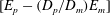
 $$\begin{eqnarray}\langle (\unicode[STIX]{x1D6E5}_{r}u_{+})^{2p}\rangle ^{1/p}=D_{p}\ln \left(\frac{r}{z}\right)+E_{p},\end{eqnarray}$$
where
 $r$
is the longitudinal distance,
$r$
is the longitudinal distance,
 $z$
the distance from the wall and
$z$
the distance from the wall and
 $D_{p}$
,
$D_{p}$
,
 $E_{p}$
are constants. Such a representation is shown in figure 1(a), which presents the longitudinal second-order structure function,
$E_{p}$
are constants. Such a representation is shown in figure 1(a), which presents the longitudinal second-order structure function,
 $\langle (\unicode[STIX]{x1D6E5}_{r}u_{+})^{2}\rangle$
, from the boundary layer databases used in the present work (see table 1 for further details). Results from each database are computed at approximately the geometric centre of the logarithmic region, which is taken to nominally span the range
$\langle (\unicode[STIX]{x1D6E5}_{r}u_{+})^{2}\rangle$
, from the boundary layer databases used in the present work (see table 1 for further details). Results from each database are computed at approximately the geometric centre of the logarithmic region, which is taken to nominally span the range
 $3\sqrt{Re_{\unicode[STIX]{x1D70F}}}<z^{+}<0.15Re_{\unicode[STIX]{x1D70F}}$
(Marusic et al.
Reference Marusic, Monty, Hultmark and Smits2013). The solid line in figure 1(a,b) reproduces the scaling described by (1.3) with the coefficients reported by de Silva et al. (Reference de Silva, Marusic, Woodcock and Meneveau2015). The results exhibit good agreement in the ECR scales (
$3\sqrt{Re_{\unicode[STIX]{x1D70F}}}<z^{+}<0.15Re_{\unicode[STIX]{x1D70F}}$
(Marusic et al.
Reference Marusic, Monty, Hultmark and Smits2013). The solid line in figure 1(a,b) reproduces the scaling described by (1.3) with the coefficients reported by de Silva et al. (Reference de Silva, Marusic, Woodcock and Meneveau2015). The results exhibit good agreement in the ECR scales (
 $z<r\ll \unicode[STIX]{x1D6FF}$
) for the high Reynolds number databases. However, even at Reynolds numbers in excess of
$z<r\ll \unicode[STIX]{x1D6FF}$
) for the high Reynolds number databases. However, even at Reynolds numbers in excess of
 $O(10^{4})$
, scaling is only present over less than a decade of
$O(10^{4})$
, scaling is only present over less than a decade of
 $r/z$
.
$r/z$
.
Further, to illustrate the influence of the wall-normal position,
 $z$
, figure 1(b) shows
$z$
, figure 1(b) shows
 $\langle (\unicode[STIX]{x1D6E5}_{r}u_{+})^{2}\rangle$
computed for the database at
$\langle (\unicode[STIX]{x1D6E5}_{r}u_{+})^{2}\rangle$
computed for the database at
 $Re_{\unicode[STIX]{x1D70F}}\approx 19\,000$
at different
$Re_{\unicode[STIX]{x1D70F}}\approx 19\,000$
at different
 $z$
within the logarithmic region. Here, it is evident that the extent of scales (following (1.3)) is impacted by the chosen
$z$
within the logarithmic region. Here, it is evident that the extent of scales (following (1.3)) is impacted by the chosen
 $z$
, with an earlier peel-off from (1.3) with increasing
$z$
, with an earlier peel-off from (1.3) with increasing
 $z$
, consistent with the scaling range
$z$
, consistent with the scaling range
 $z<r\ll \unicode[STIX]{x1D6FF}$
(Davidson, Nickels & Krogstad Reference Davidson, Nickels and Krogstad2006). Additionally, this log-law scaling is even harder to discern at
$z<r\ll \unicode[STIX]{x1D6FF}$
(Davidson, Nickels & Krogstad Reference Davidson, Nickels and Krogstad2006). Additionally, this log-law scaling is even harder to discern at
 $Re_{\unicode[STIX]{x1D70F}}\sim O(10^{3})$
for the ECR scales (to be discussed further in § 4.1), as these flows are yet to exhibit a clear logarithmic region in the variance (Smits, McKeon & Marusic Reference Smits, McKeon and Marusic2011). However, direct numerical simulation (DNS) databases at
$Re_{\unicode[STIX]{x1D70F}}\sim O(10^{3})$
for the ECR scales (to be discussed further in § 4.1), as these flows are yet to exhibit a clear logarithmic region in the variance (Smits, McKeon & Marusic Reference Smits, McKeon and Marusic2011). However, direct numerical simulation (DNS) databases at
 $Re_{\unicode[STIX]{x1D70F}}\sim O(10^{3})$
have access to volumetric, multi-component information. Therefore, if one can discern the scaling for the ECR scales from these databases it would open avenues to examine the other velocity components/directions. In this work, we will show that the universality of the scaling for the ECR scales in an ESS framework is applicable to
$Re_{\unicode[STIX]{x1D70F}}\sim O(10^{3})$
have access to volumetric, multi-component information. Therefore, if one can discern the scaling for the ECR scales from these databases it would open avenues to examine the other velocity components/directions. In this work, we will show that the universality of the scaling for the ECR scales in an ESS framework is applicable to
 $Re_{\unicode[STIX]{x1D70F}}\sim O(10^{3})$
as well as different flow geometries of wall-bounded turbulence. Previous studies (see Chung et al. (Reference Chung, Marusic, Monty, Vallikivi and Smits2015) for pipe flows and Sillero, Jiménez & Moser (Reference Sillero, Jiménez and Moser2013) for channel flows) have reported that the scaling behaviour of the ECR scales differs, based on flow geometry if one is restricted to a classical analysis.
$Re_{\unicode[STIX]{x1D70F}}\sim O(10^{3})$
as well as different flow geometries of wall-bounded turbulence. Previous studies (see Chung et al. (Reference Chung, Marusic, Monty, Vallikivi and Smits2015) for pipe flows and Sillero, Jiménez & Moser (Reference Sillero, Jiménez and Moser2013) for channel flows) have reported that the scaling behaviour of the ECR scales differs, based on flow geometry if one is restricted to a classical analysis.

Figure 1. (a) The second-order longitudinal structure function,
 $\langle (\unicode[STIX]{x1D6E5}_{r}u_{+})^{2}\rangle$
versus
$\langle (\unicode[STIX]{x1D6E5}_{r}u_{+})^{2}\rangle$
versus
 $r/z$
. The symbols represent different datasets (defined in table 1), and the results are computed at wall-normal locations within the logarithmic region: ♢:
$r/z$
. The symbols represent different datasets (defined in table 1), and the results are computed at wall-normal locations within the logarithmic region: ♢:
 $z^{+}\approx 800$
, ▵:
$z^{+}\approx 800$
, ▵:
 $z^{+}\approx 1.6\times 10^{4}$
and ●:
$z^{+}\approx 1.6\times 10^{4}$
and ●:
 $z^{+}\approx 150$
. (b)
$z^{+}\approx 150$
. (b)
 $\langle (\unicode[STIX]{x1D6E5}_{r}u_{+})^{2}\rangle$
versus
$\langle (\unicode[STIX]{x1D6E5}_{r}u_{+})^{2}\rangle$
versus
 $r/z$
at
$r/z$
at
 $Re_{\unicode[STIX]{x1D70F}}\approx 19\,000$
(♢ symbols) across the range
$Re_{\unicode[STIX]{x1D70F}}\approx 19\,000$
(♢ symbols) across the range
 $0.01<z/\unicode[STIX]{x1D6FF}<0.15$
. The solid line (——) in (a,b) corresponds to a log-law fit following (1.3) in the range
$0.01<z/\unicode[STIX]{x1D6FF}<0.15$
. The solid line (——) in (a,b) corresponds to a log-law fit following (1.3) in the range
 $z<r\ll \unicode[STIX]{x1D6FF}$
.
$z<r\ll \unicode[STIX]{x1D6FF}$
.
Table 1. Summary of experimental and numerical databases and their corresponding symbols. Databases with two symbols have access to both longitudinal and transversal information.

Throughout this paper, the coordinate system
 $x$
,
$x$
,
 $y$
and
$y$
and
 $z$
refers to the streamwise, spanwise and wall-normal directions, respectively. The corresponding instantaneous streamwise, spanwise and wall-normal velocity fluctuations are represented by
$z$
refers to the streamwise, spanwise and wall-normal directions, respectively. The corresponding instantaneous streamwise, spanwise and wall-normal velocity fluctuations are represented by
 $u$
,
$u$
,
 $v$
and
$v$
and
 $w$
.
$w$
.
2 Experimental and numerical databases
This study utilizes a collection of wall-bounded flow databases from both experimental and numerical works, which are summarized in table 1. Collectively, they cover different flow geometries (boundary layer, channel and pipe flow) and span a wide range of Reynolds numbers.
The high
 $Re$
laboratory boundary layer dataset (♢ symbols) is acquired from the High Reynolds Number Boundary Layer Wind Tunnel (HRNBLWT) at the University of Melbourne. Further details of the facility are provided in Nickels et al. (Reference Nickels, Marusic, Hafez and Chong2005). The measurement is obtained using hotwire anemometry using a
$Re$
laboratory boundary layer dataset (♢ symbols) is acquired from the High Reynolds Number Boundary Layer Wind Tunnel (HRNBLWT) at the University of Melbourne. Further details of the facility are provided in Nickels et al. (Reference Nickels, Marusic, Hafez and Chong2005). The measurement is obtained using hotwire anemometry using a
 $2.5~\unicode[STIX]{x03BC}\text{m}$
diameter Wollaston wire operated by an in-house constant-temperature anemometer. We note that this and all other databases used in the present work are acquired with a spatial resolution sufficient to resolve the turbulence intensity accurately within the logarithmic region based on the guidelines laid out by Hutchins et al. (Reference Hutchins, Nickels, Marusic and Chong2009). The highest
$2.5~\unicode[STIX]{x03BC}\text{m}$
diameter Wollaston wire operated by an in-house constant-temperature anemometer. We note that this and all other databases used in the present work are acquired with a spatial resolution sufficient to resolve the turbulence intensity accurately within the logarithmic region based on the guidelines laid out by Hutchins et al. (Reference Hutchins, Nickels, Marusic and Chong2009). The highest
 $Re$
database (▵ symbols) is acquired from the atmospheric boundary layer at the surface layer turbulence and environmental test facility (SLTEST) located in the Utah salt flats (Kunkel & Marusic Reference Kunkel and Marusic2006) again employing hot-wires positioned within the logarithmic region.
$Re$
database (▵ symbols) is acquired from the atmospheric boundary layer at the surface layer turbulence and environmental test facility (SLTEST) located in the Utah salt flats (Kunkel & Marusic Reference Kunkel and Marusic2006) again employing hot-wires positioned within the logarithmic region.
To compliment the high
 $Re$
databases from boundary layers, we include a recent numerical database of a turbulent boundary layer at
$Re$
databases from boundary layers, we include a recent numerical database of a turbulent boundary layer at
 $Re_{\unicode[STIX]{x1D70F}}\approx 1600$
(Sillero et al.
Reference Sillero, Jiménez and Moser2013). For the present study, we use seven volumetric fields with a streamwise and spanwise extent of approximately
$Re_{\unicode[STIX]{x1D70F}}\approx 1600$
(Sillero et al.
Reference Sillero, Jiménez and Moser2013). For the present study, we use seven volumetric fields with a streamwise and spanwise extent of approximately
 $1\unicode[STIX]{x1D6FF}$
and
$1\unicode[STIX]{x1D6FF}$
and
 $10\unicode[STIX]{x1D6FF}$
, respectively, thus allowing us to compute both the longitudinal (● symbols) and transversal (▸ symbols) structure functions. The final two databases are from a channel flow DNS by del Alamo et al. (Reference del Alamo, Jiménez, Zandonade and Moser2004) and a pipe flow measurement by Ng et al. (Reference Ng, Monty, Hutchins, Chong and Marusic2011). Similar to the boundary layer case, we use five volumetric fields with a streamwise and spanwise extent of
$10\unicode[STIX]{x1D6FF}$
, respectively, thus allowing us to compute both the longitudinal (● symbols) and transversal (▸ symbols) structure functions. The final two databases are from a channel flow DNS by del Alamo et al. (Reference del Alamo, Jiménez, Zandonade and Moser2004) and a pipe flow measurement by Ng et al. (Reference Ng, Monty, Hutchins, Chong and Marusic2011). Similar to the boundary layer case, we use five volumetric fields with a streamwise and spanwise extent of
 $8\unicode[STIX]{x03C0}\unicode[STIX]{x1D6FF}$
and
$8\unicode[STIX]{x03C0}\unicode[STIX]{x1D6FF}$
and
 $3\unicode[STIX]{x03C0}\unicode[STIX]{x1D6FF}$
, respectively, for the channel flow DNS. The pipe flow measurement is acquired using hot-wire anemometry in a similar fashion to the high
$3\unicode[STIX]{x03C0}\unicode[STIX]{x1D6FF}$
, respectively, for the channel flow DNS. The pipe flow measurement is acquired using hot-wire anemometry in a similar fashion to the high
 $Re$
boundary layer databases. Further details on all measurements can be found in their respective publications. We note for all the hot-wire anemometry database we use Taylor’s frozen turbulence hypothesis to convert the time-series information from the hot-wires to spatial information using the local mean velocity as the convection velocity. The validity of using Taylor’s frozen turbulence hypothesis at least up to
$Re$
boundary layer databases. Further details on all measurements can be found in their respective publications. We note for all the hot-wire anemometry database we use Taylor’s frozen turbulence hypothesis to convert the time-series information from the hot-wires to spatial information using the local mean velocity as the convection velocity. The validity of using Taylor’s frozen turbulence hypothesis at least up to
 $r<\unicode[STIX]{x1D6FF}$
is confirmed by de Silva et al. (Reference de Silva, Marusic, Woodcock and Meneveau2015). Other studies which have also assessed the accuracy of invoking Taylor’s hypothesis include Dennis & Nickels (Reference Dennis and Nickels2008), Del Alamo & Jiménez (Reference Del Alamo and Jiménez2009), Chung & McKeon (Reference Chung and McKeon2010), Atkinson, Buchmann & Soria (Reference Atkinson, Buchmann and Soria2014).
$r<\unicode[STIX]{x1D6FF}$
is confirmed by de Silva et al. (Reference de Silva, Marusic, Woodcock and Meneveau2015). Other studies which have also assessed the accuracy of invoking Taylor’s hypothesis include Dennis & Nickels (Reference Dennis and Nickels2008), Del Alamo & Jiménez (Reference Del Alamo and Jiménez2009), Chung & McKeon (Reference Chung and McKeon2010), Atkinson, Buchmann & Soria (Reference Atkinson, Buchmann and Soria2014).
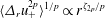
The subsequent analysis involves computing higher-order moments, therefore a brief discussion on the degree of convergence of the higher moments is warranted. The convergence of the hot-wire databases (♢, ▵ and ▫ symbols) has already been established by de Silva et al. (Reference de Silva, Marusic, Woodcock and Meneveau2015) up to
 $p=5$
or the tenth-order moment. Meanwhile, for the DNS databases, we are limited by the number of accessible volumes, therefore the premultiplied probability density function for velocity fluctuations
$p=5$
or the tenth-order moment. Meanwhile, for the DNS databases, we are limited by the number of accessible volumes, therefore the premultiplied probability density function for velocity fluctuations
 $(\unicode[STIX]{x1D6E5}_{r}u_{+})^{2p}P(\unicode[STIX]{x1D6E5}_{r}u^{+})$
is computed in order to assess the degree of convergence following the approach described in Meneveau & Marusic (Reference Meneveau and Marusic2013) and Huisman, Lohse & Sun (Reference Huisman, Lohse and Sun2013). The results are shown in figure 2 for the two DNS databases and reveal that acceptable convergence is observed up to
$(\unicode[STIX]{x1D6E5}_{r}u_{+})^{2p}P(\unicode[STIX]{x1D6E5}_{r}u^{+})$
is computed in order to assess the degree of convergence following the approach described in Meneveau & Marusic (Reference Meneveau and Marusic2013) and Huisman, Lohse & Sun (Reference Huisman, Lohse and Sun2013). The results are shown in figure 2 for the two DNS databases and reveal that acceptable convergence is observed up to
 $2p=6$
in the sense that the respective structure function of order
$2p=6$
in the sense that the respective structure function of order
 $2p$
, which is the area under the curve, is captured well (i.e. the tails of the distributions plotted in figure 2 are smooth). However, convergence at
$2p$
, which is the area under the curve, is captured well (i.e. the tails of the distributions plotted in figure 2 are smooth). However, convergence at
 $2p=8$
and beyond is moderate, therefore, for the subsequent analysis results from the DNS datasets at
$2p=8$
and beyond is moderate, therefore, for the subsequent analysis results from the DNS datasets at
 $2p>6$
should be considered with due caution.
$2p>6$
should be considered with due caution.

Figure 2. Premultiplied probability density function of
 $\unicode[STIX]{x1D6E5}_{r}u_{+}$
at
$\unicode[STIX]{x1D6E5}_{r}u_{+}$
at
 $r\approx z^{+}$
within the logarithmic region. (a,b) Correspond to the boundary layer DNS of Sillero et al. (Reference Sillero, Jiménez and Moser2013) and the channel flow DNS of del Alamo et al. (Reference del Alamo, Jiménez, Zandonade and Moser2004), respectively. The moments
$r\approx z^{+}$
within the logarithmic region. (a,b) Correspond to the boundary layer DNS of Sillero et al. (Reference Sillero, Jiménez and Moser2013) and the channel flow DNS of del Alamo et al. (Reference del Alamo, Jiménez, Zandonade and Moser2004), respectively. The moments
 $2p=2$
,
$2p=2$
,
 $6$
, and
$6$
, and
 $10$
are represented by ○, ▫ and ▵, respectively. Curves are divided by an arbitrary factor
$10$
are represented by ○, ▫ and ▵, respectively. Curves are divided by an arbitrary factor
 $K_{p}$
such that the maximum for all orders is one.
$K_{p}$
such that the maximum for all orders is one.
3 Relative relations of structure functions for the ECR scales
Based on our observations from the streamwise structure function for the ECR scales in turbulent boundary layers (see figure 1) it is evident that (1.3) holds over a very limited range of scales, even for high
 $Re$
flows of
$Re$
flows of
 $O(10^{4})$
. Therefore, in order to establish further reaching universality, we examine – in the spirit of ESS – the relative relations of the velocity structure functions. That is, rather than examining
$O(10^{4})$
. Therefore, in order to establish further reaching universality, we examine – in the spirit of ESS – the relative relations of the velocity structure functions. That is, rather than examining
 $\langle (\unicode[STIX]{x1D6E5}_{r}u_{+})^{2p}\rangle ^{1/p}$
versus
$\langle (\unicode[STIX]{x1D6E5}_{r}u_{+})^{2p}\rangle ^{1/p}$
versus
 $\log (r/z)$
as in figure 1, we plot
$\log (r/z)$
as in figure 1, we plot
 $\langle (\unicode[STIX]{x1D6E5}_{r}u_{+})^{2p}\rangle ^{1/p}$
versus
$\langle (\unicode[STIX]{x1D6E5}_{r}u_{+})^{2p}\rangle ^{1/p}$
versus
 $\langle (\unicode[STIX]{x1D6E5}_{r}u_{+})^{2m}\rangle ^{1/m}$
, thus obtaining the ratios
$\langle (\unicode[STIX]{x1D6E5}_{r}u_{+})^{2m}\rangle ^{1/m}$
, thus obtaining the ratios
 $D_{p}/D_{m}$
of the coefficients
$D_{p}/D_{m}$
of the coefficients
 $D_{p}$
from the slopes of such plots. Specifically, for the ECR scales following (1.3) we obtain the ratios
$D_{p}$
from the slopes of such plots. Specifically, for the ECR scales following (1.3) we obtain the ratios
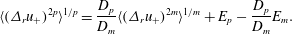 $$\begin{eqnarray}\langle (\unicode[STIX]{x1D6E5}_{r}u_{+})^{2p}\rangle ^{1/p}=\frac{D_{p}}{D_{m}}\langle (\unicode[STIX]{x1D6E5}_{r}u_{+})^{2m}\rangle ^{1/m}+E_{p}-\frac{D_{p}}{D_{m}}E_{m}.\end{eqnarray}$$
In figure 3(a) we show this type of plot for
 $\langle (\unicode[STIX]{x1D6E5}_{r}u_{+})^{4}\rangle ^{1/2}$
versus
$\langle (\unicode[STIX]{x1D6E5}_{r}u_{+})^{4}\rangle ^{1/2}$
versus
 $\langle (\unicode[STIX]{x1D6E5}_{r}u_{+})^{2}\rangle$
. Compared to the direct representation,
$\langle (\unicode[STIX]{x1D6E5}_{r}u_{+})^{2}\rangle$
. Compared to the direct representation,
 $\langle (\unicode[STIX]{x1D6E5}_{r}u_{+})^{2p}\rangle ^{1/p}$
versus
$\langle (\unicode[STIX]{x1D6E5}_{r}u_{+})^{2p}\rangle ^{1/p}$
versus
 $\log (r/z)$
(cf. figure 1
a), which was limited to the range
$\log (r/z)$
(cf. figure 1
a), which was limited to the range
 $z<r\ll \unicode[STIX]{x1D6FF}$
, the results reveal a convincingly extended scaling range beyond
$z<r\ll \unicode[STIX]{x1D6FF}$
, the results reveal a convincingly extended scaling range beyond
 $r\gtrsim z$
. Further, an accurate estimate of
$r\gtrsim z$
. Further, an accurate estimate of
 $D_{p}/D_{m}$
can now also be obtained from the lower
$D_{p}/D_{m}$
can now also be obtained from the lower
 $Re$
database at
$Re$
database at
 $Re_{\unicode[STIX]{x1D70F}}\approx 1600$
, highlighting the extended universality of (3.1) for the ECR scales. This in turn would allow us to discern the scaling coefficients of structure functions from other velocity components/directions, which are more readily accessible from databases at
$Re_{\unicode[STIX]{x1D70F}}\approx 1600$
, highlighting the extended universality of (3.1) for the ECR scales. This in turn would allow us to discern the scaling coefficients of structure functions from other velocity components/directions, which are more readily accessible from databases at
 $Re_{\unicode[STIX]{x1D70F}}\sim O(10^{3})$
. It is worth noting that if the distribution of
$Re_{\unicode[STIX]{x1D70F}}\sim O(10^{3})$
. It is worth noting that if the distribution of
 $\unicode[STIX]{x1D6E5}_{r}u$
was Gaussian, the scaling ratios would be known, i.e. then
$\unicode[STIX]{x1D6E5}_{r}u$
was Gaussian, the scaling ratios would be known, i.e. then
 $\langle (\unicode[STIX]{x1D6E5}_{r}u_{+})^{2p}\rangle ^{1/p}=[(2p-1)!!]^{1/p}\langle (\unicode[STIX]{x1D6E5}_{r}u_{+})^{2}\rangle$
. However, in the general case such a simple relation does not exist. Therefore, since
$\langle (\unicode[STIX]{x1D6E5}_{r}u_{+})^{2p}\rangle ^{1/p}=[(2p-1)!!]^{1/p}\langle (\unicode[STIX]{x1D6E5}_{r}u_{+})^{2}\rangle$
. However, in the general case such a simple relation does not exist. Therefore, since
 $\unicode[STIX]{x1D6E5}_{r}u$
is non-Gaussian (i.e. non-zero third moment, non-zero additive constant
$\unicode[STIX]{x1D6E5}_{r}u$
is non-Gaussian (i.e. non-zero third moment, non-zero additive constant
 $[E_{p}-(D_{p}/D_{m})E_{m}]$
in (3.1), see also de Silva et al. (Reference de Silva, Marusic, Woodcock and Meneveau2015)), the scaling described in (3.1) is a non-trivial result.
$[E_{p}-(D_{p}/D_{m})E_{m}]$
in (3.1), see also de Silva et al. (Reference de Silva, Marusic, Woodcock and Meneveau2015)), the scaling described in (3.1) is a non-trivial result.
As an aside, we also include the traditional ESS plot (cf. figure 3
b for reference), where
 $\langle (\unicode[STIX]{x1D6E5}_{r}u_{+})^{4}\rangle ^{1/2}$
and
$\langle (\unicode[STIX]{x1D6E5}_{r}u_{+})^{4}\rangle ^{1/2}$
and
 $\langle (\unicode[STIX]{x1D6E5}_{r}u_{+})^{2}\rangle$
are plotted on log–log scales. Benzi et al. (Reference Benzi, Ciliberto, Tripiccione, Baudet, Massaioli and Succi1993, Reference Benzi, Ciliberto, Baudet and Ruiz-Chavarria1995) have shown that in this form better estimates of the relative ISR scaling exponents,
$\langle (\unicode[STIX]{x1D6E5}_{r}u_{+})^{2}\rangle$
are plotted on log–log scales. Benzi et al. (Reference Benzi, Ciliberto, Tripiccione, Baudet, Massaioli and Succi1993, Reference Benzi, Ciliberto, Baudet and Ruiz-Chavarria1995) have shown that in this form better estimates of the relative ISR scaling exponents,
 $\unicode[STIX]{x1D701}_{p}/\unicode[STIX]{x1D701}_{m}$
, can be computed compared to the velocity structure function
$\unicode[STIX]{x1D701}_{p}/\unicode[STIX]{x1D701}_{m}$
, can be computed compared to the velocity structure function
 $\langle \unicode[STIX]{x1D6E5}_{r}u_{+}^{2p}\rangle ^{1/p}\propto r^{\unicode[STIX]{x1D701}_{2p}/p}$
itself.
$\langle \unicode[STIX]{x1D6E5}_{r}u_{+}^{2p}\rangle ^{1/p}\propto r^{\unicode[STIX]{x1D701}_{2p}/p}$
itself.

Figure 3. (a) ESS plot for
 $\langle (\unicode[STIX]{x1D6E5}_{r}u_{+})^{4}\rangle ^{1/2}$
versus
$\langle (\unicode[STIX]{x1D6E5}_{r}u_{+})^{4}\rangle ^{1/2}$
versus
 $\langle (\unicode[STIX]{x1D6E5}_{r}u_{+})^{2}\rangle$
. The symbols represent different datasets (defined in table 1), and the results are computed at wall-normal locations within the logarithmic region: ♢:
$\langle (\unicode[STIX]{x1D6E5}_{r}u_{+})^{2}\rangle$
. The symbols represent different datasets (defined in table 1), and the results are computed at wall-normal locations within the logarithmic region: ♢:
 $z^{+}\approx 800$
, ▵:
$z^{+}\approx 800$
, ▵:
 $z^{+}\approx 1.6\times 10^{4}$
and ●:
$z^{+}\approx 1.6\times 10^{4}$
and ●:
 $z^{+}\approx 150$
. The solid line (——) corresponds to a fit following (3.1) to the experimental database at
$z^{+}\approx 150$
. The solid line (——) corresponds to a fit following (3.1) to the experimental database at
 $Re_{\unicode[STIX]{x1D70F}}\approx 19\,000$
. For reference (b) shows (a) reproduced on a log–log plot in the traditional ESS form between
$Re_{\unicode[STIX]{x1D70F}}\approx 19\,000$
. For reference (b) shows (a) reproduced on a log–log plot in the traditional ESS form between
 $\langle (\unicode[STIX]{x1D6E5}_{r}u_{+})^{4}\rangle ^{1/2}$
and
$\langle (\unicode[STIX]{x1D6E5}_{r}u_{+})^{4}\rangle ^{1/2}$
and
 $\langle (\unicode[STIX]{x1D6E5}_{r}u_{+})^{2}\rangle$
.
$\langle (\unicode[STIX]{x1D6E5}_{r}u_{+})^{2}\rangle$
.

Figure 4. ESS plot for higher-order moments for the same databases shown in figure 3. (a)
 $\langle (\unicode[STIX]{x1D6E5}_{r}u_{+})^{6}\rangle ^{1/3}$
versus
$\langle (\unicode[STIX]{x1D6E5}_{r}u_{+})^{6}\rangle ^{1/3}$
versus
 $\langle (\unicode[STIX]{x1D6E5}_{r}u_{+})^{2}\rangle$
, (b)
$\langle (\unicode[STIX]{x1D6E5}_{r}u_{+})^{2}\rangle$
, (b)
 $\langle (\unicode[STIX]{x1D6E5}_{r}u_{+})^{8}\rangle ^{1/4}$
versus
$\langle (\unicode[STIX]{x1D6E5}_{r}u_{+})^{8}\rangle ^{1/4}$
versus
 $\langle (\unicode[STIX]{x1D6E5}_{r}u_{+})^{2}\rangle$
and (c)
$\langle (\unicode[STIX]{x1D6E5}_{r}u_{+})^{2}\rangle$
and (c)
 $\langle (\unicode[STIX]{x1D6E5}_{r}u_{+})^{10}\rangle ^{1/5}$
versus
$\langle (\unicode[STIX]{x1D6E5}_{r}u_{+})^{10}\rangle ^{1/5}$
versus
 $\langle (\unicode[STIX]{x1D6E5}_{r}u_{+})^{2}\rangle$
. The solid red lines (——) correspond to a fit following (3.1) to the experimental database at
$\langle (\unicode[STIX]{x1D6E5}_{r}u_{+})^{2}\rangle$
. The solid red lines (——) correspond to a fit following (3.1) to the experimental database at
 $Re_{\unicode[STIX]{x1D70F}}\approx 19\,000$
, and the values
$Re_{\unicode[STIX]{x1D70F}}\approx 19\,000$
, and the values
 $D_{p}/D_{1}$
are tabulated in table 2. (d) Ratios
$D_{p}/D_{1}$
are tabulated in table 2. (d) Ratios
 $D_{p}/D_{1}$
for the different databases. The symbols in all panels represent different datasets (defined in table 1), and the results are computed at wall-normal locations within the logarithmic region: ♢:
$D_{p}/D_{1}$
for the different databases. The symbols in all panels represent different datasets (defined in table 1), and the results are computed at wall-normal locations within the logarithmic region: ♢:
 $z^{+}\approx 800$
, ▵:
$z^{+}\approx 800$
, ▵:
 $z^{+}\approx 1.6\times 10^{4}$
and ●:
$z^{+}\approx 1.6\times 10^{4}$
and ●:
 $z^{+}\approx 150$
.
$z^{+}\approx 150$
.
To further validate the improved robustness of the scaling described in (3.1) for the ECR scales, figure 4(a–c) presents results for the even, higher-order structure functions at approximately the geometric centre of the logarithmic region. The results show good collapse of the higher-order moments up to
 $2p=10$
and provide further direct support for (3.1). To quantify these findings, figure 4(d) and table 2 present the ratios of
$2p=10$
and provide further direct support for (3.1). To quantify these findings, figure 4(d) and table 2 present the ratios of
 $D_{p}$
relative to
$D_{p}$
relative to
 $D_{m}$
(with
$D_{m}$
(with
 $m=1$
) computed based on a linear fit in the range
$m=1$
) computed based on a linear fit in the range
 $r\gtrsim z$
. We note good agreement with the coefficients reported by de Silva et al. (Reference de Silva, Marusic, Woodcock and Meneveau2015) who had access to sufficiently high
$r\gtrsim z$
. We note good agreement with the coefficients reported by de Silva et al. (Reference de Silva, Marusic, Woodcock and Meneveau2015) who had access to sufficiently high
 $Re$
databases, however, following (3.1) we can reproduce accurate estimates even for the low
$Re$
databases, however, following (3.1) we can reproduce accurate estimates even for the low
 $Re$
databases (● symbols) in the present work. Previously, databases at comparably low
$Re$
databases (● symbols) in the present work. Previously, databases at comparably low
 $Re$
would only provide a poor direct estimate of
$Re$
would only provide a poor direct estimate of
 $D_{p}$
following (1.3) (see also figure 6). Table 2 also presents estimates of the higher-order coefficients
$D_{p}$
following (1.3) (see also figure 6). Table 2 also presents estimates of the higher-order coefficients
 $D_{2-5}$
for reference from the database at
$D_{2-5}$
for reference from the database at
 $Re_{\unicode[STIX]{x1D70F}}\approx 19\,000$
, determined from the computed ratios
$Re_{\unicode[STIX]{x1D70F}}\approx 19\,000$
, determined from the computed ratios
 $D_{p}/D_{m}$
(now over a much wider range of scales,
$D_{p}/D_{m}$
(now over a much wider range of scales,
 ${\sim}r\gtrsim z$
) together with a known estimate of one coefficient (here chosen to be
${\sim}r\gtrsim z$
) together with a known estimate of one coefficient (here chosen to be
 $D_{1}$
). It should be noted that computing higher-order moments, particularly from experimental databases, can be prone to inaccuracies due to the presence of measurement noise. Nevertheless, here we observe consistent support for (3.1) across a wide range of experimental databases and numerical databases.
$D_{1}$
). It should be noted that computing higher-order moments, particularly from experimental databases, can be prone to inaccuracies due to the presence of measurement noise. Nevertheless, here we observe consistent support for (3.1) across a wide range of experimental databases and numerical databases.
Table 2. Comparison of the ratios
 $D_{p}/D_{1}$
for the ECR scales from different turbulent boundary layer datasets. The range for each
$D_{p}/D_{1}$
for the ECR scales from different turbulent boundary layer datasets. The range for each
 $D_{p}/D_{1}$
estimate indicates a 95 % confidence bound. The scaling constants,
$D_{p}/D_{1}$
estimate indicates a 95 % confidence bound. The scaling constants,
 $D_{p}$
, is presented at
$D_{p}$
, is presented at
 $Re_{\unicode[STIX]{x1D70F}}\approx 19\,000$
based on the reference value,
$Re_{\unicode[STIX]{x1D70F}}\approx 19\,000$
based on the reference value,
 $D_{1}$
(indicated by the * symbol) from the same database.
$D_{1}$
(indicated by the * symbol) from the same database.

4 Further evidence of universality
4.1 Influence of wall-normal location and flow geometry
Previously, it was highlighted that the scaling observed for the ECR scales is prevalent across a finite wall-normal extent (see figure 1). Specifically, even-order structure functions are reported to follow (1.3) within the bounds of the logarithmic region (Davidson et al.
Reference Davidson, Nickels and Krogstad2006), where self-similarity is most prevalent as bulk flow effects [
 $z\sim O(\unicode[STIX]{x1D6FF})$
] or viscous effects [
$z\sim O(\unicode[STIX]{x1D6FF})$
] or viscous effects [
 $z^{+}\sim O(1)$
] are minimal. Recent work on moment generating functions by Yang et al. (Reference Yang, Meneveau, Marusic and Biferale2016b
) has shown that the extent of logarithmic scaling as a function of
$z^{+}\sim O(1)$
] are minimal. Recent work on moment generating functions by Yang et al. (Reference Yang, Meneveau, Marusic and Biferale2016b
) has shown that the extent of logarithmic scaling as a function of
 $z$
increases when examining ratios between moment generating functions in ESS form. They postulated that bulk flow or viscous effects would affect all moment generating functions similarly, therefore, their ratio would exhibit a larger self-similarity region. Here, we explore if the structure functions also exhibit similar behaviour at the ECR scales, with an extended wall-normal extent following (3.1).
$z$
increases when examining ratios between moment generating functions in ESS form. They postulated that bulk flow or viscous effects would affect all moment generating functions similarly, therefore, their ratio would exhibit a larger self-similarity region. Here, we explore if the structure functions also exhibit similar behaviour at the ECR scales, with an extended wall-normal extent following (3.1).
To this end, figure 5(a) presents the sixth-order structure function,
 $\langle (\unicode[STIX]{x1D6E5}_{r}u_{+})^{6}\rangle ^{1/3}$
, versus spatial separation
$\langle (\unicode[STIX]{x1D6E5}_{r}u_{+})^{6}\rangle ^{1/3}$
, versus spatial separation
 $r$
across the entire boundary layer for the dataset at
$r$
across the entire boundary layer for the dataset at
 $Re_{\unicode[STIX]{x1D70F}}=19\,000$
. We note that the sixth-order structure function is chosen as a representative case to highlight any subtle differences as a function of wall-normal height, when plotted in the ESS framework. Each line corresponds to
$Re_{\unicode[STIX]{x1D70F}}=19\,000$
. We note that the sixth-order structure function is chosen as a representative case to highlight any subtle differences as a function of wall-normal height, when plotted in the ESS framework. Each line corresponds to
 $\langle (\unicode[STIX]{x1D6E5}_{r}u_{+})^{6}\rangle ^{1/3}$
computed at a fixed wall-normal (
$\langle (\unicode[STIX]{x1D6E5}_{r}u_{+})^{6}\rangle ^{1/3}$
computed at a fixed wall-normal (
 $z$
) location within the range
$z$
) location within the range
 $10<z^{+}<Re_{\unicode[STIX]{x1D70F}}$
. The results show that even at
$10<z^{+}<Re_{\unicode[STIX]{x1D70F}}$
. The results show that even at
 $Re_{\unicode[STIX]{x1D70F}}\sim O(10^{4})$
a log law for the ECR scales is only discernible within the logarithmic region, which are highlighted by the red lines (——). Figure 5(b) reproduces the same statistics across the entire boundary layer for
$Re_{\unicode[STIX]{x1D70F}}\sim O(10^{4})$
a log law for the ECR scales is only discernible within the logarithmic region, which are highlighted by the red lines (——). Figure 5(b) reproduces the same statistics across the entire boundary layer for
 $\langle (\unicode[STIX]{x1D6E5}_{r}u_{+})^{6}\rangle ^{1/3}$
, but now as a function of
$\langle (\unicode[STIX]{x1D6E5}_{r}u_{+})^{6}\rangle ^{1/3}$
, but now as a function of
 $\langle (\unicode[STIX]{x1D6E5}_{r}u_{+})^{2}\rangle$
. The results exhibit encouraging collapse across a much larger wall-normal extent (
$\langle (\unicode[STIX]{x1D6E5}_{r}u_{+})^{2}\rangle$
. The results exhibit encouraging collapse across a much larger wall-normal extent (
 $z^{+}\gtrsim 50$
) following (3.1) compared to directly examining
$z^{+}\gtrsim 50$
) following (3.1) compared to directly examining
 $\langle (\unicode[STIX]{x1D6E5}_{r}u_{+})^{6}\rangle ^{1/3}$
versus spatial separation
$\langle (\unicode[STIX]{x1D6E5}_{r}u_{+})^{6}\rangle ^{1/3}$
versus spatial separation
 $r$
. We note that beyond
$r$
. We note that beyond
 $z^{+}\gtrsim 50$
the multiplicative constant, i.e. the ratio
$z^{+}\gtrsim 50$
the multiplicative constant, i.e. the ratio
 $D_{p}/D_{1}$
, appears unchanged, while the additive constant in (3.1) has a subtle trend with
$D_{p}/D_{1}$
, appears unchanged, while the additive constant in (3.1) has a subtle trend with
 $z$
. In any case, in the ESS inspired framework, we are able to discern the scaling coefficients (slopes
$z$
. In any case, in the ESS inspired framework, we are able to discern the scaling coefficients (slopes
 $D_{p}/D_{1}$
) of the ECR scales more accurately, particularly at low Reynolds numbers when no clear logarithmic region exists.
$D_{p}/D_{1}$
) of the ECR scales more accurately, particularly at low Reynolds numbers when no clear logarithmic region exists.

Figure 5. (a)
 $\langle (\unicode[STIX]{x1D6E5}_{r}u_{+})^{6}\rangle ^{1/3}$
versus
$\langle (\unicode[STIX]{x1D6E5}_{r}u_{+})^{6}\rangle ^{1/3}$
versus
 $r/z$
at all available wall-normal (
$r/z$
at all available wall-normal (
 $z$
) locations from the hot-wire dataset of Hutchins et al. (Reference Hutchins, Nickels, Marusic and Chong2009) at
$z$
) locations from the hot-wire dataset of Hutchins et al. (Reference Hutchins, Nickels, Marusic and Chong2009) at
 $Re_{\unicode[STIX]{x1D70F}}\approx 19\,000$
. Each line corresponds to different
$Re_{\unicode[STIX]{x1D70F}}\approx 19\,000$
. Each line corresponds to different
 $z$
locations from the wall up to
$z$
locations from the wall up to
 $z/\unicode[STIX]{x1D6FF}\approx 1$
with darker shading corresponding to higher
$z/\unicode[STIX]{x1D6FF}\approx 1$
with darker shading corresponding to higher
 $z$
. The red lines (——) highlight
$z$
. The red lines (——) highlight
 $z$
locations within the logarithmic region. The blue dashed line (– –) corresponds to the scaling law expected for the ECR scales. (b) Shows (a) reproduced now as a relation between
$z$
locations within the logarithmic region. The blue dashed line (– –) corresponds to the scaling law expected for the ECR scales. (b) Shows (a) reproduced now as a relation between
 $\langle (\unicode[STIX]{x1D6E5}_{r}u_{+})^{6}\rangle ^{1/3}$
and
$\langle (\unicode[STIX]{x1D6E5}_{r}u_{+})^{6}\rangle ^{1/3}$
and
 $\langle (\unicode[STIX]{x1D6E5}_{r}u_{+})^{2}\rangle$
, revealing universality.
$\langle (\unicode[STIX]{x1D6E5}_{r}u_{+})^{2}\rangle$
, revealing universality.

Figure 6. (a)
 $\langle (\unicode[STIX]{x1D6E5}_{r}u_{+})^{4}\rangle ^{1/2}$
versus
$\langle (\unicode[STIX]{x1D6E5}_{r}u_{+})^{4}\rangle ^{1/2}$
versus
 $r/z$
computed from boundary layers, pipes and channel flows at different
$r/z$
computed from boundary layers, pipes and channel flows at different
 $Re$
. The symbols represent different datasets (defined in table 1), and the results are computed at wall-normal locations within the logarithmic region: ♢:
$Re$
. The symbols represent different datasets (defined in table 1), and the results are computed at wall-normal locations within the logarithmic region: ♢:
 $z^{+}\approx 800$
, ▵:
$z^{+}\approx 800$
, ▵:
 $z^{+}\approx 1.6\times 10^{4}$
, ●:
$z^{+}\approx 1.6\times 10^{4}$
, ●:
 $z^{+}\approx 150$
, ▫:
$z^{+}\approx 150$
, ▫:
 $z^{+}\approx 200$
and
$z^{+}\approx 200$
and
 $z^{+}\approx 110$
. (b)
$z^{+}\approx 110$
. (b)
 $\langle (\unicode[STIX]{x1D6E5}_{r}u_{+})^{4}\rangle ^{1/2}$
versus
$\langle (\unicode[STIX]{x1D6E5}_{r}u_{+})^{4}\rangle ^{1/2}$
versus
 $\langle (\unicode[STIX]{x1D6E5}_{r}u_{+})^{2}\rangle$
for all the datasets shown in (a), again displaying enhanced universality as compared to (a). The solid red lines (——) in (a,b) corresponds to the scaling law expected for the ECR scales.
$\langle (\unicode[STIX]{x1D6E5}_{r}u_{+})^{2}\rangle$
for all the datasets shown in (a), again displaying enhanced universality as compared to (a). The solid red lines (——) in (a,b) corresponds to the scaling law expected for the ECR scales.
Scaling of the ECR scales for different flow geometries in wall-bounded turbulence has been a subject of interest over the last decade (e.g. Monty et al.
Reference Monty, Hutchins, Ng, Marusic and Chong2009). Most works have placed emphasis on examining the spectral energy distribution (Jiménez Reference Jiménez2012). More recently, Chung et al. (Reference Chung, Marusic, Monty, Vallikivi and Smits2015) compared structure functions for pipe flow and boundary layers over a wide range of
 $Re$
and highlighted a notably shallower slope,
$Re$
and highlighted a notably shallower slope,
 $D_{1}$
, for pipe flows, which was less discernible for pipe flows with increasing
$D_{1}$
, for pipe flows, which was less discernible for pipe flows with increasing
 $Re$
. To highlight these differences due to flow geometry, figure 6(a) presents
$Re$
. To highlight these differences due to flow geometry, figure 6(a) presents
 $\langle (\unicode[STIX]{x1D6E5}_{r}u_{+})^{4}\rangle ^{1/2}$
from pipes, channels and boundary layers. Results for the three flow geometries are presented at a comparable
$\langle (\unicode[STIX]{x1D6E5}_{r}u_{+})^{4}\rangle ^{1/2}$
from pipes, channels and boundary layers. Results for the three flow geometries are presented at a comparable
 $Re_{\unicode[STIX]{x1D70F}}$
(
$Re_{\unicode[STIX]{x1D70F}}$
(
 ${\sim}$
1000–3000) and are computed at approximately the geometric centre of the logarithmic region. The results show clear evidence that the ECR scales exhibit different scaling behaviour indicating that the flow geometry does play a role. However, once plotted as a ratio between structure functions of different orders (see figure 6
b), good collapse is observed across the three flow geometries considered in the present work. Hence, these findings show further reaching universality for the scaling of the ECR scales for different flow geometries in wall turbulence, even at
${\sim}$
1000–3000) and are computed at approximately the geometric centre of the logarithmic region. The results show clear evidence that the ECR scales exhibit different scaling behaviour indicating that the flow geometry does play a role. However, once plotted as a ratio between structure functions of different orders (see figure 6
b), good collapse is observed across the three flow geometries considered in the present work. Hence, these findings show further reaching universality for the scaling of the ECR scales for different flow geometries in wall turbulence, even at
 $Re_{\unicode[STIX]{x1D70F}}=O(10^{3})$
when presented using an ESS inspired framework. Therefore, we postulate that even though the influence of geometrical effects (such as ‘crowding’ in pipe flows, Chung et al.
Reference Chung, Marusic, Monty, Vallikivi and Smits2015) is likely to exist in structure functions at different orders, we are still able to accurately quantify the scaling of the ratios between two structure functions (
$Re_{\unicode[STIX]{x1D70F}}=O(10^{3})$
when presented using an ESS inspired framework. Therefore, we postulate that even though the influence of geometrical effects (such as ‘crowding’ in pipe flows, Chung et al.
Reference Chung, Marusic, Monty, Vallikivi and Smits2015) is likely to exist in structure functions at different orders, we are still able to accurately quantify the scaling of the ratios between two structure functions (
 $D_{p}/D_{m}$
) for the ECR scales. Moreover, if one has an accurate estimate of the scaling constants for
$D_{p}/D_{m}$
) for the ECR scales. Moreover, if one has an accurate estimate of the scaling constants for
 $\langle (\unicode[STIX]{x1D6E5}_{r}u_{+})^{2}\rangle$
, the behaviour of the higher-order counterparts, can be estimated using the ratios presented in table 2.
$\langle (\unicode[STIX]{x1D6E5}_{r}u_{+})^{2}\rangle$
, the behaviour of the higher-order counterparts, can be estimated using the ratios presented in table 2.
To further validate the improved robustness of the scaling described in (3.1) for the ECR scales over different flow geometries, figure 7(a,b) presents
 $\langle (\unicode[STIX]{x1D6E5}_{r}u_{+})^{4}\rangle ^{1/2}$
as a function of
$\langle (\unicode[STIX]{x1D6E5}_{r}u_{+})^{4}\rangle ^{1/2}$
as a function of
 $\langle (\unicode[STIX]{x1D6E5}_{r}u_{+})^{2}\rangle$
computed further away from the wall at
$\langle (\unicode[STIX]{x1D6E5}_{r}u_{+})^{2}\rangle$
computed further away from the wall at
 $z\approx 0.15\unicode[STIX]{x1D6FF}$
and
$z\approx 0.15\unicode[STIX]{x1D6FF}$
and
 $z\approx 0.5\unicode[STIX]{x1D6FF}$
, respectively. The results show good agreement between all the databases exhibiting universality beyond the logarithmic region. Furthermore, the slope of the scaling law (
$z\approx 0.5\unicode[STIX]{x1D6FF}$
, respectively. The results show good agreement between all the databases exhibiting universality beyond the logarithmic region. Furthermore, the slope of the scaling law (
 $D_{2}/D_{1}$
) expected for the ECR scales (solid red line, ——) is nominally constant, albeit with a subtle shift in the additive constants,
$D_{2}/D_{1}$
) expected for the ECR scales (solid red line, ——) is nominally constant, albeit with a subtle shift in the additive constants,
 $E_{p}-(D_{p}/D_{m})E_{m}$
, in (3.1) with increasing
$E_{p}-(D_{p}/D_{m})E_{m}$
, in (3.1) with increasing
 $z$
.
$z$
.

Figure 7. (a,b)
 $\langle (\unicode[STIX]{x1D6E5}_{r}u_{+})^{4}\rangle ^{1/2}$
versus
$\langle (\unicode[STIX]{x1D6E5}_{r}u_{+})^{4}\rangle ^{1/2}$
versus
 $\langle (\unicode[STIX]{x1D6E5}_{r}u_{+})^{2}\rangle$
computed at
$\langle (\unicode[STIX]{x1D6E5}_{r}u_{+})^{2}\rangle$
computed at
 $z\approx 0.15\unicode[STIX]{x1D6FF}$
and
$z\approx 0.15\unicode[STIX]{x1D6FF}$
and
 $z\approx 0.5\unicode[STIX]{x1D6FF}$
, respectively. The symbols represent different datasets (defined in table 1). The solid red lines (——) in (a,b) are identical and correspond to the scaling law estimated for the ECR scales following (3.1) in the logarithmic region.
$z\approx 0.5\unicode[STIX]{x1D6FF}$
, respectively. The symbols represent different datasets (defined in table 1). The solid red lines (——) in (a,b) are identical and correspond to the scaling law estimated for the ECR scales following (3.1) in the logarithmic region.
4.2 Transversal structure functions in wall-bounded turbulence
The preceding discussions have shown that by plotting the ratios between longitudinal structure functions of different orders further reaching universality can be achieved for the scaling behaviour of the ECR scales, now even at
 $Re_{\unicode[STIX]{x1D70F}}=O(10^{3})$
. Therefore, it would be interesting to explore if this universality also extends to the transversal structure function at the ECR scales (see e.g. Grossmann et al. (Reference Grossmann, Lohse and Reeh1997b
), van de Water & Herweijer (Reference van de Water and Herweijer1999), Kurien et al. (Reference Kurien, Lvov, Procaccia and Sreenivasan2000), Jacob et al. (Reference Jacob, Biferale, Iuso and Casciola2004) for a discussion on the scaling for the ISR scales), which is more readily accessible at
$Re_{\unicode[STIX]{x1D70F}}=O(10^{3})$
. Therefore, it would be interesting to explore if this universality also extends to the transversal structure function at the ECR scales (see e.g. Grossmann et al. (Reference Grossmann, Lohse and Reeh1997b
), van de Water & Herweijer (Reference van de Water and Herweijer1999), Kurien et al. (Reference Kurien, Lvov, Procaccia and Sreenivasan2000), Jacob et al. (Reference Jacob, Biferale, Iuso and Casciola2004) for a discussion on the scaling for the ISR scales), which is more readily accessible at
 $Re_{\unicode[STIX]{x1D70F}}=O(10^{3})$
from numerical databases. Here the transversal structure function,
$Re_{\unicode[STIX]{x1D70F}}=O(10^{3})$
from numerical databases. Here the transversal structure function,
 $\langle (\unicode[STIX]{x1D6E5}_{r}u_{+})^{2p}\rangle _{T}^{1/p}$
, is defined following (1.1) with
$\langle (\unicode[STIX]{x1D6E5}_{r}u_{+})^{2p}\rangle _{T}^{1/p}$
, is defined following (1.1) with
 $\boldsymbol{i}$
replaced by a unit vector
$\boldsymbol{i}$
replaced by a unit vector
 $\boldsymbol{j}$
in the spanwise direction.
$\boldsymbol{j}$
in the spanwise direction.

Figure 8. (a)
 $\langle (\unicode[STIX]{x1D6E5}_{r}u_{+})^{4}\rangle ^{1/2}$
versus
$\langle (\unicode[STIX]{x1D6E5}_{r}u_{+})^{4}\rangle ^{1/2}$
versus
 $r/z$
computed from boundary layers in the longitudinal and transversal directions. The symbols represent different datasets (defined in table 1), and the results are computed at wall-normal locations within the logarithmic region: ♢:
$r/z$
computed from boundary layers in the longitudinal and transversal directions. The symbols represent different datasets (defined in table 1), and the results are computed at wall-normal locations within the logarithmic region: ♢:
 $z^{+}\approx 800$
and ▸, ●:
$z^{+}\approx 800$
and ▸, ●:
 $z^{+}\approx 150$
. (b) The transversal and longitudinal structure functions as a function of their respective second-order structure functions, i.e.
$z^{+}\approx 150$
. (b) The transversal and longitudinal structure functions as a function of their respective second-order structure functions, i.e.
 $\langle (\unicode[STIX]{x1D6E5}_{r}u_{+})^{4}\rangle ^{1/2}$
versus
$\langle (\unicode[STIX]{x1D6E5}_{r}u_{+})^{4}\rangle ^{1/2}$
versus
 $\langle (\unicode[STIX]{x1D6E5}_{r}u_{+})^{2}\rangle$
and
$\langle (\unicode[STIX]{x1D6E5}_{r}u_{+})^{2}\rangle$
and
 $\langle (\unicode[STIX]{x1D6E5}_{r}u_{+})^{4}\rangle _{T}^{1/2}$
versus
$\langle (\unicode[STIX]{x1D6E5}_{r}u_{+})^{4}\rangle _{T}^{1/2}$
versus
 $\langle (\unicode[STIX]{x1D6E5}_{r}u_{+})^{2}\rangle _{T}$
. The solid red lines (——) in (a,b) corresponds to the scaling law expected for the ECR scales.
$\langle (\unicode[STIX]{x1D6E5}_{r}u_{+})^{2}\rangle _{T}$
. The solid red lines (——) in (a,b) corresponds to the scaling law expected for the ECR scales.
Figure 8(a) presents both the fourth-order longitudinal and transversal structure functions for a turbulent boundary layer. The results show that the transversal structure function,
 $\langle (\unicode[STIX]{x1D6E5}_{r}u_{+})^{4}\rangle _{T}^{1/2}$
, also appears to exhibit a log law for the ECR scales, albeit with a sharper slope (higher
$\langle (\unicode[STIX]{x1D6E5}_{r}u_{+})^{4}\rangle _{T}^{1/2}$
, also appears to exhibit a log law for the ECR scales, albeit with a sharper slope (higher
 $D_{p}$
) compared to its longitudinal counterpart. Similar trends have also been reported by Lee & Moser (Reference Lee and Moser2015) and Chandran et al. (Reference Chandran, Baidya, Monty and Marusic2017) who examined the streamwise velocity component in the transversal and longitudinal directions. Their results are presented at a comparable
$D_{p}$
) compared to its longitudinal counterpart. Similar trends have also been reported by Lee & Moser (Reference Lee and Moser2015) and Chandran et al. (Reference Chandran, Baidya, Monty and Marusic2017) who examined the streamwise velocity component in the transversal and longitudinal directions. Their results are presented at a comparable
 $Re$
in wall-bounded turbulence but used the
$Re$
in wall-bounded turbulence but used the
 $u$
spectrogram as a diagnostic instead of structure functions to extract the scaling behaviour of the ECR scales (see Davidson et al.
Reference Davidson, Nickels and Krogstad2006). However, based on predictions from the attached eddy model, scaling of both the longitudinal and transversal directions should be equivalent for wall turbulence at high
$u$
spectrogram as a diagnostic instead of structure functions to extract the scaling behaviour of the ECR scales (see Davidson et al.
Reference Davidson, Nickels and Krogstad2006). However, based on predictions from the attached eddy model, scaling of both the longitudinal and transversal directions should be equivalent for wall turbulence at high
 $Re$
. Databases to confirm this directly are still unavailable. Nevertheless, once the transversal and longitudinal structure functions are plotted in an ESS inspired form (see figure 8
b), even at
$Re$
. Databases to confirm this directly are still unavailable. Nevertheless, once the transversal and longitudinal structure functions are plotted in an ESS inspired form (see figure 8
b), even at
 $Re_{\unicode[STIX]{x1D70F}}=O(10^{3})$
, we observe good agreement between the two for the ECR scales following (3.1). This further highlights that (3.1) is a more robust diagnostic to seek the scaling of the ECR scales.
$Re_{\unicode[STIX]{x1D70F}}=O(10^{3})$
, we observe good agreement between the two for the ECR scales following (3.1). This further highlights that (3.1) is a more robust diagnostic to seek the scaling of the ECR scales.
5 Concluding remarks
This work presents evidence of further reaching universality for the ECR scales in wall turbulence by utilising the extended self-similarity hypothesis, i.e. the relative scaling of velocity structure functions. First, the expected scaling for the ratios between velocity structure functions is outlined based on the previously reported log-law scaling for the ECR scales in high Reynolds number boundary layers (Davidson et al.
Reference Davidson, Nickels and Krogstad2006; de Silva et al.
Reference de Silva, Marusic, Woodcock and Meneveau2015). These predictions are then examined using a range of wall turbulence databases, which span a wide range of Reynolds numbers and flow geometries. The results reveal that the scaling behaviour for the ECR scales extends over a much larger range of scales (
 $r\gtrsim z$
), leading to more precise measurements of the scaling exponents. Further, it is evident that these quantitative measures can now be confidently estimated from databases at much lower Reynolds numbers and over a much larger wall-normal extent than previously thought possible.
$r\gtrsim z$
), leading to more precise measurements of the scaling exponents. Further, it is evident that these quantitative measures can now be confidently estimated from databases at much lower Reynolds numbers and over a much larger wall-normal extent than previously thought possible.
Our results also exhibit better universality for the ECR scales across different flow geometries, which before had been claimed to differ, particularly at low/modest Reynolds numbers. This universality for the ECR scales also appears to extend to the transversal streamwise structure function once plotted in ESS form. The latter is in support of the attached eddy model, which predicts equal scaling for both the longitudinal and transversal structure function at sufficiently high Reynolds numbers. A crucial next step would be to show the connection between the universal coefficients
 $D_{n}/D_{1}$
and the universal intermittency exponents
$D_{n}/D_{1}$
and the universal intermittency exponents
 $\unicode[STIX]{x1D709}_{n}$
through some matching conditions between ECR and ISR, but this will be a challenging task.
$\unicode[STIX]{x1D709}_{n}$
through some matching conditions between ECR and ISR, but this will be a challenging task.
Acknowledgements
D.L. thanks the Melbourne group for its hospitality during his visits there. Continuous financial support by the ARC, Dutch NWO and from ERC is gratefully acknowledged. D.K. acknowledges financial support by the University of Melbourne through the McKenzie fellowship.


