


1. Introduction
Wind-driven waves are usually seen as a well-understood phenomenon of which the physics appears ‘self-evident’: waves are growing due to wind and dissipate due to wave breaking. This ‘common-sense’ understanding of sea wave physics is reflected in conventional scaling of wave growth by wind speed (e.g. Sverdrup & Munk Reference Sverdrup and Munk1947; Kitaigorodskii Reference Kitaigorodskii1962) and in attempts to find features of wave growth universality in terms of such scaling. The non-dimensional wave height variance
 ${\it\varepsilon}$
(wave energy in the wave community terminology) and the non-dimensional characteristic wave frequency, defined respectively by
${\it\varepsilon}$
(wave energy in the wave community terminology) and the non-dimensional characteristic wave frequency, defined respectively by
 $$\begin{eqnarray}\displaystyle {\it\varepsilon}=\frac{Eg^{2}}{U_{h}^{4}} & & \displaystyle\end{eqnarray}$$
 $$\begin{eqnarray}\displaystyle {\it\sigma}=\frac{\tilde{{\it\omega}}U_{h}}{g}, & & \displaystyle\end{eqnarray}$$
 $g$
, the wind speed
$g$
, the wind speed
 $U_{h}$
at a reference height
$U_{h}$
at a reference height
 $h$
or the friction velocity
$h$
or the friction velocity
 $u^{\ast }$
(for a constant-flux turbulent boundary layer
$u^{\ast }$
(for a constant-flux turbulent boundary layer
 $u^{\ast }=(\langle U^{\prime }W^{\prime }\rangle )^{1/2}$
), and the wave height variance
$u^{\ast }=(\langle U^{\prime }W^{\prime }\rangle )^{1/2}$
), and the wave height variance
 $E=\langle |{\it\eta}|^{2}\rangle$
, are widely used in experimental and numerical studies. The characteristic wave frequency
$E=\langle |{\it\eta}|^{2}\rangle$
, are widely used in experimental and numerical studies. The characteristic wave frequency
 $\tilde{{\it\omega}}$
in (1.2) can be defined as the mean-over-spectrum frequency
$\tilde{{\it\omega}}$
in (1.2) can be defined as the mean-over-spectrum frequency
 ${\it\omega}_{m}$
, the zero-crossing
${\it\omega}_{m}$
, the zero-crossing
 ${\it\omega}_{z}$
or the spectral peak frequency
${\it\omega}_{z}$
or the spectral peak frequency
 ${\it\omega}_{p}$
. Below we refer to the spectral peak frequency
${\it\omega}_{p}$
. Below we refer to the spectral peak frequency
 ${\it\omega}_{p}$
as the characteristic one unless otherwise stated.
${\it\omega}_{p}$
as the characteristic one unless otherwise stated.
Quite often results of wave studies are recapitulated in the form of power-law functions of the dimensionless time duration
 ${\it\tau}=tg/U_{h}$
or the fetch
${\it\tau}=tg/U_{h}$
or the fetch
 ${\it\chi}=xg/U_{h}^{2}$
, as follows:
${\it\chi}=xg/U_{h}^{2}$
, as follows:
 $$\begin{eqnarray}\displaystyle {\it\varepsilon}={\it\varepsilon}_{0}{\it\tau}^{p_{{\it\tau}}},\quad {\it\sigma}={\it\sigma}_{0}{\it\tau}^{-q_{{\it\tau}}};\quad {\it\varepsilon}={\it\varepsilon}_{0}{\it\chi}^{p_{{\it\chi}}},\quad {\it\sigma}={\it\sigma}_{0}{\it\chi}^{-q_{{\it\chi}}}, & & \displaystyle\end{eqnarray}$$
that already implies, in a manner, a universality of wind wave growth. However, the coefficients
 ${\it\varepsilon}_{0},{\it\sigma}_{0}$
and the exponents
${\it\varepsilon}_{0},{\it\sigma}_{0}$
and the exponents
 $p_{{\it\tau}}(p_{{\it\chi}}),q_{{\it\tau}}(q_{{\it\chi}})$
of such parameterizations vary in a relatively wide range (e.g.
$p_{{\it\tau}}(p_{{\it\chi}}),q_{{\it\tau}}(q_{{\it\chi}})$
of such parameterizations vary in a relatively wide range (e.g.
 $0.7<p_{{\it\chi}}<1.1$
, see table 2 Badulin et al.
Reference Badulin, Babanin, Resio and Zakharov2007a
).
$0.7<p_{{\it\chi}}<1.1$
, see table 2 Badulin et al.
Reference Badulin, Babanin, Resio and Zakharov2007a
).
We consider that the very fact of a power-like dependence of energy and representative frequency on fetch and duration is significant and requires a theoretical explanation. A number of reasons can be called upon to explain the lack of complete universality: the inadequacy of the power-law fit, the complexity of wind–wave interaction, the irrelevance of scaling by a mean wind speed with no account of the air flow stratification, gustiness etc. All these issues imply a leading effect of wind forcing rather than accounting for all the complexity of wind–sea dynamics. It leaves (intentionally or unintentionally) the inherently nonlinear dynamics of wind waves at the periphery of the discussion.
In this paper we come back to the fundamental problem of the balance between the various physical mechanisms governing wind-wave growth. In contrast to the conventional ‘common-sense’ understanding of this well-known natural phenomenon we develop an alternative paradigm of weakly turbulent wind-driven seas where the universality of wind-wave growth is determined, first of all, by the features of nonlinear wave–wave interactions in a random field of water waves. These features cause a strong tendency of wind-driven seas to self-similar behaviour as shown theoretically, in simulations and in analysis of experimental data (Badulin et al. Reference Badulin, Pushkarev, Resio and Zakharov2002, Reference Badulin, Pushkarev, Resio and Zakharov2005, Reference Badulin, Babanin, Resio and Zakharov2007a , Reference Badulin, Babanin, Resio, Zakharov, Borisov, Kozlov, Mamaev and Sokolovskiy2008; Gagnaire-Renou, Benoit & Badulin Reference Gagnaire-Renou, Benoit and Badulin2011). The corresponding theory predicts power-law dependence of wave energy and characteristic frequency on dimensionless duration or fetch very similar to the conventional parameterizations (1.3). The distinctiveness of the theoretical approach lies in offering an alternative scaling for describing wind-wave development that does not refer directly to wind speed.
Here we show that for duration- and fetch-limited setups wind-wave growth can be presented in a remarkably concise, but somewhat paradoxical, form that does not contain parameters of wind at all, namely
 $$\begin{eqnarray}{\it\mu}^{4}{\it\nu}={\it\alpha}_{0}^{3},\end{eqnarray}$$
where
 ${\it\alpha}_{0}\approx 0.7$
is a universal constant and
${\it\alpha}_{0}\approx 0.7$
is a universal constant and
 ${\it\mu}$
, the wave steepness, is given by
${\it\mu}$
, the wave steepness, is given by
 $$\begin{eqnarray}{\it\mu}=\frac{E^{1/2}{\it\omega}_{p}^{2}}{g}.\end{eqnarray}$$
The ‘number of waves’
 ${\it\nu}$
in a spatially homogeneous wind sea (i.e. for duration-limited wave growth) is defined as follows:
${\it\nu}$
in a spatially homogeneous wind sea (i.e. for duration-limited wave growth) is defined as follows:
 $$\begin{eqnarray}{\it\nu}={\it\omega}_{p}t.\end{eqnarray}$$
For spatial (fetch-limited) wave growth the coefficient of proportionality
 $C_{f}$
that appears in the equivalent expression
$C_{f}$
that appears in the equivalent expression
 ${\it\nu}=C_{f}|\boldsymbol{k}_{p}|x$
(
${\it\nu}=C_{f}|\boldsymbol{k}_{p}|x$
(
 $\boldsymbol{k}_{p}$
being the wavevector of the spectral peak) is close to the ratio between the phase and group velocities
$\boldsymbol{k}_{p}$
being the wavevector of the spectral peak) is close to the ratio between the phase and group velocities
 $C_{ph}/C_{g}=2$
. The universal constant
$C_{ph}/C_{g}=2$
. The universal constant
 ${\it\alpha}_{0}$
in (1.4) is an analogue of the Kolmogorov–Zakharov constant of wave turbulence theory (e.g. Zakharov, Lvov & Falkovich Reference Zakharov, Lvov and Falkovich1992; Badulin et al.
Reference Badulin, Babanin, Resio and Zakharov2007a
).
${\it\alpha}_{0}$
in (1.4) is an analogue of the Kolmogorov–Zakharov constant of wave turbulence theory (e.g. Zakharov, Lvov & Falkovich Reference Zakharov, Lvov and Falkovich1992; Badulin et al.
Reference Badulin, Babanin, Resio and Zakharov2007a
).
The relationship (1.4) can be re-written as a function of one dependent variable (e.g.
 ${\it\mu}$
) of another independent variable (e.g.
${\it\mu}$
) of another independent variable (e.g.
 ${\it\nu}$
); thus, it becomes a good predictive tool. An evident advantage (and surprising outcome) is that all the necessary information on wind-generated wave growth is contained in the wave data and no wind measurement is necessary for describing the wave field evolution.
${\it\nu}$
); thus, it becomes a good predictive tool. An evident advantage (and surprising outcome) is that all the necessary information on wind-generated wave growth is contained in the wave data and no wind measurement is necessary for describing the wave field evolution.
Note that the dependence on wind speed can be excluded from empirical power-law fits (1.3) and a counterpart of our key result can be written in the spirit of (1.4) as follows:
 $$\begin{eqnarray}{\it\mu}^{4}{\it\nu}^{r}={\it\beta}({\it\varepsilon}_{0},{\it\sigma}_{0}),\end{eqnarray}$$
where for the duration-limited case (subscript
 ${\it\tau}$
)
${\it\tau}$
)
 $$\begin{eqnarray}r_{{\it\tau}}=\frac{8q_{{\it\tau}}-2p_{{\it\tau}}}{1-q_{{\it\tau}}}\end{eqnarray}$$
and for the fetch-limited setup one has (subscript
 ${\it\chi}$
)
${\it\chi}$
)
 $$\begin{eqnarray}r_{{\it\chi}}=\frac{8q_{{\it\chi}}-2p_{{\it\chi}}}{1-2q_{{\it\chi}}}.\end{eqnarray}$$
In contrast to the theoretically based relationship (1.4) the alternative one (1.7) is not universal in two ways: the exponent
 $r$
is dependent on an empirical wave growth rate and the empirical pre-exponents
$r$
is dependent on an empirical wave growth rate and the empirical pre-exponents
 ${\it\varepsilon}_{0},{\it\sigma}_{0}$
vary in a wide range as mentioned above. Thus, the physical roots of (1.4) can be discussed in terms of mechanisms that are responsible for the universal exponent
${\it\varepsilon}_{0},{\it\sigma}_{0}$
vary in a wide range as mentioned above. Thus, the physical roots of (1.4) can be discussed in terms of mechanisms that are responsible for the universal exponent
 $r$
of the number of waves
$r$
of the number of waves
 ${\it\nu}$
being equated to
${\it\nu}$
being equated to
 $1$
in (1.7) and that makes the right-hand-side term
$1$
in (1.7) and that makes the right-hand-side term
 ${\it\beta}$
in (1.7) independent of wave input features. The essence of these mechanisms can be summarized in the two following issues:
${\it\beta}$
in (1.7) independent of wave input features. The essence of these mechanisms can be summarized in the two following issues:
-
(i) the dominance of nonlinear interactions in the energy balance in wind-driven seas pre-determines the essential physical links that make (1.4) a universal law without any explicit reference to wind parameters;
-
(ii) the ubiquity of self-similar regimes in wind-driven seas (e.g. Badulin et al. Reference Badulin, Pushkarev, Resio and Zakharov2005, Reference Badulin, Babanin, Resio and Zakharov2007a ; Zakharov Reference Zakharov2005; Gagnaire-Renou et al. Reference Gagnaire-Renou, Benoit and Badulin2011) makes the invariant (1.4) an efficient tool for physical analysis of experimental and numerical results.
In this paper, we start with a brief theoretical overview of the basic physics that leads us to the key result (1.4). More details can be found in the paper series (e.g. Badulin et al. Reference Badulin, Pushkarev, Resio and Zakharov2002, Reference Badulin, Pushkarev, Resio and Zakharov2005, Reference Badulin, Babanin, Resio and Zakharov2007a , Reference Badulin, Babanin, Resio, Zakharov, Borisov, Kozlov, Mamaev and Sokolovskiy2008; Pushkarev, Resio & Zakharov Reference Pushkarev, Resio and Zakharov2003; Zakharov Reference Zakharov2005, Reference Zakharov2010).
Then we present the key result of this work, the wind-free invariant (1.4), and introduce the corresponding wind-free scaling of wave growth. A number of theoretical–empirical models of wave growth are based essentially on the physical scale of wind speed and power-law dependence of dimensionless wave height on wave period. These models and their reference exponents are well known as the Toba (Reference Toba1972) law of
 $3/2$
, Hasselmann et al. (Reference Hasselmann, Ross, Müller and Sell1976) law of
$3/2$
, Hasselmann et al. (Reference Hasselmann, Ross, Müller and Sell1976) law of
 $5/3$
and Zakharov & Zaslavsky (Reference Zakharov and Zaslavsky1983) law of
$5/3$
and Zakharov & Zaslavsky (Reference Zakharov and Zaslavsky1983) law of
 $4/3$
. We show that the physical scales of time duration or fetch are able to replace the conventional wind speed scaling fairly well. The corresponding dependence within the new scaling gives two different exponents, namely
$4/3$
. We show that the physical scales of time duration or fetch are able to replace the conventional wind speed scaling fairly well. The corresponding dependence within the new scaling gives two different exponents, namely
 $5/2$
for fetch- and
$5/2$
for fetch- and
 $9/4$
for duration-limited cases. A key outcome of the new scaling is in eliminating any question on features of wind–wave coupling when the mean wind speed alone cannot reflect the complexity of this coupling in full.
$9/4$
for duration-limited cases. A key outcome of the new scaling is in eliminating any question on features of wind–wave coupling when the mean wind speed alone cannot reflect the complexity of this coupling in full.
The simple relationship (1.4) and the new wind-free scaling are verified in several examples presented in this study. All the data for the verification of the theoretical result have been obtained prior to this work. We, thus, revisit a collection of in situ observations (see Hwang Reference Hwang2006; Hwang, Garciá-Nava & Ocampo-Torres Reference Hwang, Garciá-Nava and Ocampo-Torres2011, and references therein), simulations by Badulin et al. (Reference Badulin, Pushkarev, Resio and Zakharov2002, Reference Badulin, Pushkarev, Resio and Zakharov2005, Reference Badulin, Babanin, Resio and Zakharov2007a , Reference Badulin, Babanin, Resio, Zakharov, Borisov, Kozlov, Mamaev and Sokolovskiy2008), Zakharov, Resio & Pushkarev (Reference Zakharov, Resio and Pushkarev2012) and wind-wave tank experiments by Toba (Reference Toba1972), Caulliez (Reference Caulliez2013). A historical tour to the brilliant work by Sverdrup & Munk (Reference Sverdrup and Munk1947) brings back the concept of significant wave height as an effective alternative to the spectral description of wind seas.
In the final section we recapitulate the various validations of the universal relationship in order to show their logical links and to outline prospects for further studies.
2. Invariant form of the self-similar solutions for growing wind seas
The core of our theoretical approach is the concept of self-similar wind-driven seas. Vladimir Zakharov was the first who reported the theoretical background and experimental illustrations of the concept (Zakharov Reference Zakharov2002). It took three years for the paper to find a publisher (Zakharov Reference Zakharov2005). In parallel, the ideas of the paper have been developed and supported by extensive numerical analysis (Badulin et al. Reference Badulin, Pushkarev, Resio and Zakharov2002, Reference Badulin, Pushkarev, Resio and Zakharov2005, Reference Badulin, Babanin, Resio and Zakharov2007a ,Reference Badulin, Babanin, Resio and Zakharov b , Reference Badulin, Babanin, Resio, Zakharov, Borisov, Kozlov, Mamaev and Sokolovskiy2008; Pushkarev et al. Reference Pushkarev, Resio and Zakharov2003; Korotkevich et al. Reference Korotkevich, Pushkarev, Resio and Zakharov2008) based on the exact simulation of spectral nonlinear transfer with the algorithm by Webb (Reference Webb1978, see also Tracy & Resio Reference Tracy and Resio1982). Independently, some features of the self-similar evolution of wind-wave spectra have been justified in Lavrenov, Resio & Zakharov (Reference Lavrenov, Resio and Zakharov2002), Lavrenov (Reference Lavrenov2003a ) using an alternative numerical approach, the so-called Gaussian quadrature method (GQM).
Originally, the concept of self-similarity was developed for approximate solutions of the kinetic equation. Recently, exact self-similar solutions have been presented for specific functions of wind-wave external forcing (Zakharov et al. Reference Zakharov, Resio and Pushkarev2012; Pushkarev & Zakharov Reference Pushkarev and Zakharov2015). These input functions provide rather good fits to available empirical parameterizations and, thus, have prospects for various applications in wave modelling.
Note that self-similarity of wind seas was implied by many previous approaches, starting with the concept of significant wave height by Sverdrup & Munk (Reference Sverdrup and Munk1947), developed as a similarity approach in Kitaigorodskii (Reference Kitaigorodskii1962) and Pierson & Moskowitz (Reference Pierson and Moskowitz1964) and then in substantial generalization of experimental and theoretical knowledge in the JONSWAP campaign (Hasselmann et al. Reference Hasselmann, Barnett, Bouws, Carlson, Cartwright, Enke, Ewing, Gienapp, Hasselmann, Kruseman, Meerburg, Muller, Olbers, Richter, Sell and Walden1973). The distinctiveness of the Zakharov (Reference Zakharov2005) approach that we follow in this paper is a consistent physical theory that leads to analytical results for this extremely complicated problem where such results are rare.
2.1. The physical model of self-similar wind-driven seas
We follow a statistical description of a random field of weakly nonlinear wind-driven waves under the effect of wind forcing and wave dissipation. The spectral density of the wave action
 $N(\boldsymbol{k},\boldsymbol{x},t)$
as a function of wavenumber
$N(\boldsymbol{k},\boldsymbol{x},t)$
as a function of wavenumber
 $\boldsymbol{k}$
, spatial coordinate
$\boldsymbol{k}$
, spatial coordinate
 $\boldsymbol{x}=(x,y)$
and time
$\boldsymbol{x}=(x,y)$
and time
 $t$
can be described by the kinetic equation (Hasselmann Reference Hasselmann1962) as follows:
$t$
can be described by the kinetic equation (Hasselmann Reference Hasselmann1962) as follows:
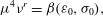
 $$\begin{eqnarray}\frac{\partial N_{\boldsymbol{k}}}{\partial t}+\boldsymbol{{\rm\nabla}}_{\boldsymbol{k}}{\it\omega}_{\boldsymbol{k}}\boldsymbol{{\rm\nabla}}_{\boldsymbol{x}}N_{\boldsymbol{k}}=S_{nl}[N(\boldsymbol{k})]+S_{in}+S_{diss}.\end{eqnarray}$$
The idea of a balance between wind input
 $S_{in}$
, wave dissipation
$S_{in}$
, wave dissipation
 $S_{diss}$
and wave–wave interactions
$S_{diss}$
and wave–wave interactions
 $S_{nl}$
has been circulating since long before World War II (e.g. Sverdrup & Munk Reference Sverdrup and Munk1947; Lavrenov Reference Lavrenov2003b
). The start of the modern concept of the spectral balance of a wind-wave field is usually attributed to the paper by Gelci, Cazalé & Vassal (Reference Gelci, Cazalé and Vassal1957) where all the terms in (2.1) have been treated as wave-scale dependent.
$S_{nl}$
has been circulating since long before World War II (e.g. Sverdrup & Munk Reference Sverdrup and Munk1947; Lavrenov Reference Lavrenov2003b
). The start of the modern concept of the spectral balance of a wind-wave field is usually attributed to the paper by Gelci, Cazalé & Vassal (Reference Gelci, Cazalé and Vassal1957) where all the terms in (2.1) have been treated as wave-scale dependent.
The milestone papers of the early 1960s by Klauss Hasselmann (Reference Hasselmann1962, Reference Hasselmann1963a
,Reference Hasselmann
b
) provided a consistent physical description of the term for four-wave resonant interactions
 $S_{nl}$
. The role of these interactions in the evolution of wind-driven waves has been recognized but has not been realized in full. The basic results of the theory of weak turbulence of water waves (Zakharov & Filonenko Reference Zakharov and Filonenko1966; Katz & Kontorovich Reference Katz and Kontorovich1971; Katz et al.
Reference Katz, Kontorovich, Moiseev and Novikov1975; Zakharov & Zaslavsky Reference Zakharov and Zaslavsky1983; Zakharov et al.
Reference Zakharov, Lvov and Falkovich1992) including those for the anisotropic Kolmogorov–Zakharov spectra (Katz & Kontorovich Reference Katz and Kontorovich1974) remained outside the chief topics studied by the wind-wave community. The efforts were focused mostly on numerical aspects of accounting for the effect of wave–wave interactions in operational and research models.
$S_{nl}$
. The role of these interactions in the evolution of wind-driven waves has been recognized but has not been realized in full. The basic results of the theory of weak turbulence of water waves (Zakharov & Filonenko Reference Zakharov and Filonenko1966; Katz & Kontorovich Reference Katz and Kontorovich1971; Katz et al.
Reference Katz, Kontorovich, Moiseev and Novikov1975; Zakharov & Zaslavsky Reference Zakharov and Zaslavsky1983; Zakharov et al.
Reference Zakharov, Lvov and Falkovich1992) including those for the anisotropic Kolmogorov–Zakharov spectra (Katz & Kontorovich Reference Katz and Kontorovich1974) remained outside the chief topics studied by the wind-wave community. The efforts were focused mostly on numerical aspects of accounting for the effect of wave–wave interactions in operational and research models.
The knowledge today of the terms
 $S_{in}$
and
$S_{in}$
and
 $S_{diss}$
on the right-hand side of (2.1) is based mostly on empirical parameterizations. This represents an additional problem for wind-wave studies when correct modelling of wave evolution requires tuning to the features of a particular environment. Below we present results that do not depend on these features and do not contain any parameters of wave generation or dissipation explicitly. The physical roots of this surprising result lie in the leading role of the wave–wave interaction term
$S_{diss}$
on the right-hand side of (2.1) is based mostly on empirical parameterizations. This represents an additional problem for wind-wave studies when correct modelling of wave evolution requires tuning to the features of a particular environment. Below we present results that do not depend on these features and do not contain any parameters of wave generation or dissipation explicitly. The physical roots of this surprising result lie in the leading role of the wave–wave interaction term
 $S_{nl}$
(e.g. Hasselmann et al.
Reference Hasselmann, Barnett, Bouws, Carlson, Cartwright, Enke, Ewing, Gienapp, Hasselmann, Kruseman, Meerburg, Muller, Olbers, Richter, Sell and Walden1973; Young & van Vledder Reference Young and van Vledder1993; Badulin et al.
Reference Badulin, Pushkarev, Resio and Zakharov2005; Zakharov & Badulin Reference Zakharov and Badulin2011): the effects of external forcing appear directly embedded in the intrinsic parameters of the nonlinear wave field.
$S_{nl}$
(e.g. Hasselmann et al.
Reference Hasselmann, Barnett, Bouws, Carlson, Cartwright, Enke, Ewing, Gienapp, Hasselmann, Kruseman, Meerburg, Muller, Olbers, Richter, Sell and Walden1973; Young & van Vledder Reference Young and van Vledder1993; Badulin et al.
Reference Badulin, Pushkarev, Resio and Zakharov2005; Zakharov & Badulin Reference Zakharov and Badulin2011): the effects of external forcing appear directly embedded in the intrinsic parameters of the nonlinear wave field.
Following the previous works (e.g. Badulin et al.
Reference Badulin, Pushkarev, Resio and Zakharov2005, Reference Badulin, Babanin, Resio and Zakharov2007a
; Zakharov Reference Zakharov2005) we consider an asymptotic model describing the wind-driven seas. Assuming wave–wave interactions to be dominant compared to wind forcing and wave dissipation one can split (2.1) into two equations. In terms of the spectral energy density
 $E(\boldsymbol{k},\boldsymbol{x},t)$
the model takes the form
$E(\boldsymbol{k},\boldsymbol{x},t)$
the model takes the form
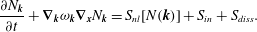
 $$\begin{eqnarray}\displaystyle \frac{\text{d}E_{k}}{\text{d}t} & = & \displaystyle S_{nl},\end{eqnarray}$$
 $$\begin{eqnarray}\displaystyle \frac{\text{d}\langle E_{k}\rangle }{\text{d}t} & = & \displaystyle \langle S_{in}+S_{diss}\rangle .\end{eqnarray}$$
A breakthrough can be made for deep water waves when the wave dispersion relation and the wave–wave interaction term
 $S_{nl}$
are homogeneous functions of the spectral energy density
$S_{nl}$
are homogeneous functions of the spectral energy density
 $E(\boldsymbol{k},\boldsymbol{x},t)$
and the wave vector
$E(\boldsymbol{k},\boldsymbol{x},t)$
and the wave vector
 $\boldsymbol{k}$
, i.e.
$\boldsymbol{k}$
, i.e.
 $$\begin{eqnarray}S_{nl}[{\it\upsilon}E({\it\varrho}\boldsymbol{k})]={\it\upsilon}^{3}{\it\varrho}^{17/2}S_{nl}[E(\boldsymbol{k})],\end{eqnarray}$$
with
 ${\it\upsilon}$
and
${\it\upsilon}$
and
 ${\it\varrho}$
being arbitrary positive coefficients (e.g. Zakharov Reference Zakharov1999). This important property allows one to look for self-similar solutions as function of time (fetch) and wave frequency (wavenumber).
${\it\varrho}$
being arbitrary positive coefficients (e.g. Zakharov Reference Zakharov1999). This important property allows one to look for self-similar solutions as function of time (fetch) and wave frequency (wavenumber).
2.2. Power-law dependence of the self-similar solutions
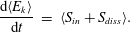
Now we briefly outline features of self-similar solutions for the system (2.2), details being given in appendix A. Let us introduce dimensionless variables for the model (2.2) as follows (Badulin et al. Reference Badulin, Pushkarev, Resio and Zakharov2005, Reference Badulin, Babanin, Resio and Zakharov2007a ; Zakharov Reference Zakharov2005):
 $$\begin{eqnarray}\displaystyle \left.\begin{array}{@{}c@{}}{\bf\chi}=\boldsymbol{x}/l_{0},\quad \tilde{\boldsymbol{k}}=\boldsymbol{k}l_{0},\\ {\it\tau}=t/t_{0},\quad \tilde{{\it\omega}}={\it\omega}\sqrt{l_{0}/g}=\sqrt{|\tilde{\boldsymbol{k}}|},\\ \tilde{E}(\tilde{\boldsymbol{k}})=E(\boldsymbol{k})/l_{0}^{4},\quad \tilde{E}(\boldsymbol{k})=E/l_{0}^{2}.\end{array}\right\} & & \displaystyle\end{eqnarray}$$
Note that the time and length scales
 $t_{0}$
and
$t_{0}$
and
 $l_{0}$
can be chosen arbitrarily in the deep water case, say, by accepting wind speed scaling (1.1), (1.2) as an option (e.g. Hwang Reference Hwang2006).
$l_{0}$
can be chosen arbitrarily in the deep water case, say, by accepting wind speed scaling (1.1), (1.2) as an option (e.g. Hwang Reference Hwang2006).
For the duration-limited setup one has in (2.2)
 $$\begin{eqnarray}\displaystyle \frac{\text{d}}{\text{d}t}\rightarrow \frac{\partial }{\partial t}, & & \displaystyle\end{eqnarray}$$
and the solution in the form of the so-called incomplete self-similarity can be written as
 $$\begin{eqnarray}\tilde{E}(\tilde{\boldsymbol{k}},{\it\tau})=a_{{\it\tau}}{\it\tau}^{p_{{\it\tau}}+4q_{{\it\tau}}}{\it\Phi}_{p_{{\it\tau}}}({\bf\xi}),\end{eqnarray}$$
where
 ${\bf\xi}=b_{{\it\tau}}\boldsymbol{k}t^{2q_{{\it\tau}}}$
. Substitution of (2.6) into (2.2) leads to two constraints on parameters
${\bf\xi}=b_{{\it\tau}}\boldsymbol{k}t^{2q_{{\it\tau}}}$
. Substitution of (2.6) into (2.2) leads to two constraints on parameters
 $p_{{\it\tau}},q_{{\it\tau}}$
and
$p_{{\it\tau}},q_{{\it\tau}}$
and
 $a_{{\it\tau}},b_{{\it\tau}}$
that are of key importance for further analysis. Thus, energy growth and frequency downshift are governed by the linear relationship
$a_{{\it\tau}},b_{{\it\tau}}$
that are of key importance for further analysis. Thus, energy growth and frequency downshift are governed by the linear relationship
 $$\begin{eqnarray}q_{{\it\tau}}=\frac{2p_{{\it\tau}}+1}{9},\end{eqnarray}$$
while the parameters of the solution amplitude
 $a_{{\it\tau}}$
and its width in wavenumber space
$a_{{\it\tau}}$
and its width in wavenumber space
 $b_{{\it\tau}}$
obey the equation
$b_{{\it\tau}}$
obey the equation
 $$\begin{eqnarray}a_{{\it\tau}}=b_{{\it\tau}}^{17/4}.\end{eqnarray}$$
These useful relationships confirm empirical power-like laws (1.3a,b ) with
 $$\begin{eqnarray}{\it\varepsilon}_{0}=a_{{\it\tau}}^{9/17}I_{{\it\tau}},\quad {\it\sigma}_{0}=a_{{\it\tau}}^{-2/17}J_{{\it\tau}}I_{{\it\tau}}^{-1}.\end{eqnarray}$$
Here
 $I_{{\it\tau}},J_{{\it\tau}}$
(see (A 3), (A 5) in appendix A) are integral expressions of the shape function
$I_{{\it\tau}},J_{{\it\tau}}$
(see (A 3), (A 5) in appendix A) are integral expressions of the shape function
 ${\it\Phi}_{p_{{\it\tau}}}({\bf\xi})$
in (2.6) that do not depend on exponent
${\it\Phi}_{p_{{\it\tau}}}({\bf\xi})$
in (2.6) that do not depend on exponent
 $p_{{\it\tau}}$
explicitly. After combining relationships (1.3a,b
), (2.7), (2.9) in the form of the invariant (1.4) we observe a remarkable outcome: the result does not depend on time and initial state (i.e. on pre-exponent
$p_{{\it\tau}}$
explicitly. After combining relationships (1.3a,b
), (2.7), (2.9) in the form of the invariant (1.4) we observe a remarkable outcome: the result does not depend on time and initial state (i.e. on pre-exponent
 $a_{{\it\tau}}$
). Moreover, its implicit dependence on exponent
$a_{{\it\tau}}$
). Moreover, its implicit dependence on exponent
 $p_{{\it\tau}}$
is expressed by integrals of the shape function
$p_{{\it\tau}}$
is expressed by integrals of the shape function
 ${\it\Phi}_{p_{{\it\tau}}}({\bf\xi})$
. Assuming spectral shape invariance, i.e. integrals
${\it\Phi}_{p_{{\it\tau}}}({\bf\xi})$
. Assuming spectral shape invariance, i.e. integrals
 $I_{{\it\tau}},J_{{\it\tau}}$
to be constants, we get immediately that
$I_{{\it\tau}},J_{{\it\tau}}$
to be constants, we get immediately that
 ${\it\alpha}_{0}$
in (1.4) is constant. This is what we call the universality of wind-driven seas.
${\it\alpha}_{0}$
in (1.4) is constant. This is what we call the universality of wind-driven seas.
Note that the assumption of spectral shape invariance is introduced here for the integral quantities
 $I_{{\it\tau}}$
and
$I_{{\it\tau}}$
and
 $J_{{\it\tau}}$
and is not equivalent to a point-by-point matching of the shape functions
$J_{{\it\tau}}$
and is not equivalent to a point-by-point matching of the shape functions
 ${\it\Phi}_{p_{{\it\tau}}}({\bf\xi})$
for different exponents
${\it\Phi}_{p_{{\it\tau}}}({\bf\xi})$
for different exponents
 $p_{{\it\tau}}$
. This assumption has been carefully checked in previous extensive numerical studies (Badulin et al.
Reference Badulin, Pushkarev, Resio and Zakharov2005, Reference Badulin, Babanin, Resio and Zakharov2007a
, Reference Badulin, Babanin, Resio, Zakharov, Borisov, Kozlov, Mamaev and Sokolovskiy2008). A similar assumption has been exploited by Hasselmann et al. (Reference Hasselmann, Ross, Müller and Sell1976, see § 2).
$p_{{\it\tau}}$
. This assumption has been carefully checked in previous extensive numerical studies (Badulin et al.
Reference Badulin, Pushkarev, Resio and Zakharov2005, Reference Badulin, Babanin, Resio and Zakharov2007a
, Reference Badulin, Babanin, Resio, Zakharov, Borisov, Kozlov, Mamaev and Sokolovskiy2008). A similar assumption has been exploited by Hasselmann et al. (Reference Hasselmann, Ross, Müller and Sell1976, see § 2).
The same universal behaviour holds in the fetch-limited setup. Now one has
 $$\begin{eqnarray}\displaystyle \frac{\text{d}}{\text{d}t}\rightarrow \frac{\partial {\it\omega}}{\partial k}\frac{\partial }{\partial x}, & & \displaystyle\end{eqnarray}$$
and the self-similar solution is given by the expression
 $$\begin{eqnarray}\tilde{E}(\tilde{\boldsymbol{k}},{\it\chi})=a_{{\it\chi}}{\it\chi}^{p_{{\it\chi}}+4q_{{\it\chi}}}{\it\Phi}_{p_{{\it\chi}}}({\bf\zeta}),\end{eqnarray}$$
with
 ${\bf\zeta}=b_{{\it\chi}}\tilde{\boldsymbol{k}}\tilde{x}^{2q_{{\it\chi}}}$
. Again, substitution into (2.2) gives links between exponents
${\bf\zeta}=b_{{\it\chi}}\tilde{\boldsymbol{k}}\tilde{x}^{2q_{{\it\chi}}}$
. Again, substitution into (2.2) gives links between exponents
 $$\begin{eqnarray}q_{{\it\chi}}=\frac{2p_{{\it\chi}}+1}{10}\end{eqnarray}$$
and pre-exponents
 $$\begin{eqnarray}a_{{\it\chi}}=b_{{\it\chi}}^{9/2}.\end{eqnarray}$$
Similarly to the duration-limited case the pre-exponents of wave growth in (1.3c,d ) are
 $$\begin{eqnarray}{\it\varepsilon}_{0}=a_{{\it\chi}}^{5/9}I_{{\it\chi}},\quad {\it\sigma}_{0}=a_{{\it\chi}}^{-1/9}J_{{\it\chi}}I_{{\it\chi}}^{-1}.\end{eqnarray}$$
It is easy to check that the invariant (1.4) keeps the same form as the one in the duration-limited case with the number of waves
 ${\it\nu}$
defined in terms of spatial wave period. Again, the invariant does not depend on time and initial state (i.e. on pre-exponent
${\it\nu}$
defined in terms of spatial wave period. Again, the invariant does not depend on time and initial state (i.e. on pre-exponent
 $a_{{\it\chi}}$
). The implicit dependence of the integrals
$a_{{\it\chi}}$
). The implicit dependence of the integrals
 $I_{{\it\chi}}$
and
$I_{{\it\chi}}$
and
 $J_{{\it\chi}}$
in (A 10), (A 13) on exponent
$J_{{\it\chi}}$
in (A 10), (A 13) on exponent
 $p_{{\it\chi}}$
is weak and the assumption of spectral shape invariance can be accepted to fix the right-hand-side value as constant
$p_{{\it\chi}}$
is weak and the assumption of spectral shape invariance can be accepted to fix the right-hand-side value as constant
 ${\it\alpha}_{0}$
.
${\it\alpha}_{0}$
.
2.3. Universal constant
 ${\it\alpha}_{0}$
for duration- and fetch-limited setups
${\it\alpha}_{0}$
for duration- and fetch-limited setups

The importance of links between parameters of self-similar solutions (2.7), (2.8), (2.12), (2.13) was first realized by Badulin et al. (Reference Badulin, Babanin, Resio and Zakharov2007a , see (1.9)) in the form of the so-called weakly turbulent law of wind-wave growth
 $$\begin{eqnarray}\frac{E{\it\omega}_{p}^{4}}{g^{2}}={\it\alpha}_{ss}\left(\frac{{\it\omega}_{p}^{3}\,\text{d}E/\text{d}t}{g^{2}}\right)^{1/3}.\end{eqnarray}$$
Here
 ${\it\alpha}_{ss}$
is a coefficient that depends on the exponent of wave energy growth
${\it\alpha}_{ss}$
is a coefficient that depends on the exponent of wave energy growth
 $p_{{\it\tau}}$
(
$p_{{\it\tau}}$
(
 $p_{{\it\chi}}$
) only. Assuming spectral shape invariance (quasi-universality of spectral shape in the words of Badulin et al.
Reference Badulin, Babanin, Resio and Zakharov2007a
) one obtains
$p_{{\it\chi}}$
) only. Assuming spectral shape invariance (quasi-universality of spectral shape in the words of Badulin et al.
Reference Badulin, Babanin, Resio and Zakharov2007a
) one obtains
 ${\it\alpha}_{ss}\sim p_{{\it\tau}}^{-1/3}$
(
${\it\alpha}_{ss}\sim p_{{\it\tau}}^{-1/3}$
(
 ${\it\alpha}_{ss}\sim p_{{\it\chi}}^{-1/3}$
). For a given parameter
${\it\alpha}_{ss}\sim p_{{\it\chi}}^{-1/3}$
). For a given parameter
 $p_{{\it\tau}}(p_{{\it\chi}})$
, i.e. for a power-law growth of wave energy, the relationship (2.15) allows for the conversion of the instant wave energy and frequency into the instant wave input or vice versa (see § 5 in Badulin et al.
Reference Badulin, Babanin, Resio and Zakharov2007a
).
$p_{{\it\tau}}(p_{{\it\chi}})$
, i.e. for a power-law growth of wave energy, the relationship (2.15) allows for the conversion of the instant wave energy and frequency into the instant wave input or vice versa (see § 5 in Badulin et al.
Reference Badulin, Babanin, Resio and Zakharov2007a
).
In contrast to
 ${\it\alpha}_{ss}$
in (2.15),
${\it\alpha}_{ss}$
in (2.15),
 ${\it\alpha}_{0}$
in the invariant (1.4) is constant (with the assumption of spectral shape invariance) and the invariant itself does not contain time or space derivatives but physical quantities that we are interested in only (wave height and period). Thus, the conservation law (1.4) can be treated as an adiabatic invariant for (2.15) and for the corresponding families of self-similar solutions of the model (2.2) with
${\it\alpha}_{0}$
in the invariant (1.4) is constant (with the assumption of spectral shape invariance) and the invariant itself does not contain time or space derivatives but physical quantities that we are interested in only (wave height and period). Thus, the conservation law (1.4) can be treated as an adiabatic invariant for (2.15) and for the corresponding families of self-similar solutions of the model (2.2) with
 $p_{{\it\tau}}(p_{{\it\chi}})$
being formally a slowly varying parameter. The features of this adiabatic invariant are, first, independence of the parameter of adiabaticity
$p_{{\it\tau}}(p_{{\it\chi}})$
being formally a slowly varying parameter. The features of this adiabatic invariant are, first, independence of the parameter of adiabaticity
 $p_{{\it\tau}}(p_{{\it\chi}})$
and, secondly, independence of the initial state of the system. The first one implies an arbitrary dependence of wave growth on time or fetch. The second feature looks strange amongst examples of classic mechanics when a conservative quantity, say the wave action of an oscillator, is determined by its initial energy and frequency. In fact, our special case reflects an asymptotic nature of the self-similar solutions of the kinetic equation and their inherent nonlinearity that forces the system to forget the initial state.
$p_{{\it\tau}}(p_{{\it\chi}})$
and, secondly, independence of the initial state of the system. The first one implies an arbitrary dependence of wave growth on time or fetch. The second feature looks strange amongst examples of classic mechanics when a conservative quantity, say the wave action of an oscillator, is determined by its initial energy and frequency. In fact, our special case reflects an asymptotic nature of the self-similar solutions of the kinetic equation and their inherent nonlinearity that forces the system to forget the initial state.
It is useful to specify different values of the constant
 ${\it\alpha}_{0}$
in (1.4) for duration- and fetch-limited setups. The correspondence of these cases comes directly from the relationships between the partial derivative in time and the convective operator in the model (2.2), i.e.
${\it\alpha}_{0}$
in (1.4) for duration- and fetch-limited setups. The correspondence of these cases comes directly from the relationships between the partial derivative in time and the convective operator in the model (2.2), i.e.
 $$\begin{eqnarray}\displaystyle \frac{\text{d}}{\text{d}t}\rightarrow \frac{\partial }{\partial t}\rightarrow V\frac{\partial }{\partial x}. & & \displaystyle\end{eqnarray}$$
The velocity
 $V$
is associated with averaging the wave energy flux over the wave-scale range, i.e.
$V$
is associated with averaging the wave energy flux over the wave-scale range, i.e.
 $$\begin{eqnarray}\displaystyle \langle C_{g}(\boldsymbol{k})E(\boldsymbol{k})\rangle =V\langle E(\boldsymbol{k})\rangle . & & \displaystyle\end{eqnarray}$$
Generally,
 $V$
differs from the group velocity of the spectral peak given by
$V$
differs from the group velocity of the spectral peak given by
 $$\begin{eqnarray}\displaystyle C_{g}({\it\omega}_{p})=0.5\frac{g}{{\it\omega}_{p}}, & & \displaystyle\end{eqnarray}$$
a quantity we are exploiting in our analysis. This case allows a simple definition of the number of waves
 ${\it\nu}$
in the fetch-limited case, that is
${\it\nu}$
in the fetch-limited case, that is
 $$\begin{eqnarray}{\it\nu}=2|\boldsymbol{k}_{p}|x,\end{eqnarray}$$
which will be used below in this paper for the fetch-limited case. Furthermore, to check the law (1.4) we take the definitions (1.6) and (2.19) for duration- and fetch-limited cases respectively as follows:
 $$\begin{eqnarray}{\it\mu}^{4}{\it\nu}={\it\alpha}_{0(d)}^{3}\quad \text{or}\quad {\it\mu}^{4}{\it\nu}={\it\alpha}_{0(f)}^{3}.\end{eqnarray}$$
The notation
 ${\it\alpha}_{0}$
without the extended subscript is used below provided this does not lead to confusion. Following Badulin et al. (Reference Badulin, Babanin, Resio and Zakharov2007a
) and Gagnaire-Renou et al. (Reference Gagnaire-Renou, Benoit and Badulin2011) one can obtain the two estimates
${\it\alpha}_{0}$
without the extended subscript is used below provided this does not lead to confusion. Following Badulin et al. (Reference Badulin, Babanin, Resio and Zakharov2007a
) and Gagnaire-Renou et al. (Reference Gagnaire-Renou, Benoit and Badulin2011) one can obtain the two estimates
 $$\begin{eqnarray}\displaystyle {\it\alpha}_{0(d)}={\it\alpha}_{ss}^{(d)}p_{{\it\tau}}^{1/3}\approx 0.70, & & \displaystyle\end{eqnarray}$$
 $$\begin{eqnarray}\displaystyle {\it\alpha}_{0(f)}={\it\alpha}_{ss}^{(f)}p_{{\it\chi}}^{1/3}\approx 0.62. & & \displaystyle\end{eqnarray}$$
 ${\it\alpha}_{0(d)}$
and
${\it\alpha}_{0(d)}$
and
 ${\it\alpha}_{0(f)}$
can be partially related to the difference in shape of the wave spectra of duration- and fetch-limited seas. This is unlikely to be the major effect if we accept spectral shape invariance. It is more natural to treat the small (about 10 %) difference as one between the characteristic velocity
${\it\alpha}_{0(f)}$
can be partially related to the difference in shape of the wave spectra of duration- and fetch-limited seas. This is unlikely to be the major effect if we accept spectral shape invariance. It is more natural to treat the small (about 10 %) difference as one between the characteristic velocity
 $V$
and the group velocity of the spectral peak. If we are looking for a ‘perfect universality’ of our law, i.e. equivalence between
$V$
and the group velocity of the spectral peak. If we are looking for a ‘perfect universality’ of our law, i.e. equivalence between
 ${\it\alpha}_{0(f)}$
and
${\it\alpha}_{0(f)}$
and
 ${\it\alpha}_{0(d)}$
, we have to take into account this difference between
${\it\alpha}_{0(d)}$
, we have to take into account this difference between
 $V$
and
$V$
and
 $C_{g}({\it\omega}_{p})$
in the definition of the number of waves
$C_{g}({\it\omega}_{p})$
in the definition of the number of waves
 ${\it\nu}$
in (2.19), i.e.
${\it\nu}$
in (2.19), i.e.  $$\begin{eqnarray}\frac{V}{C_{g}({\it\omega}_{p})}=\left(\frac{{\it\alpha}_{0(f)}}{{\it\alpha}_{0(d)}}\right)^{3}\approx 0.7.\end{eqnarray}$$
The characteristic velocity
 $V$
for wind-wave spectra appears to be approximately 30 % smaller than that of the spectral peak
$V$
for wind-wave spectra appears to be approximately 30 % smaller than that of the spectral peak
 $C_{g}({\it\omega}_{p})$
which matches quite well with previous experimental results (e.g. Yefimov & Babanin Reference Yefimov and Babanin1991; Hwang & Wang Reference Hwang and Wang2004; Hwang Reference Hwang2006).
$C_{g}({\it\omega}_{p})$
which matches quite well with previous experimental results (e.g. Yefimov & Babanin Reference Yefimov and Babanin1991; Hwang & Wang Reference Hwang and Wang2004; Hwang Reference Hwang2006).
3. Physical scaling of growing wind seas and the first test of the universality of wind-wave growth
The theoretical results of the previous section look paradoxical and contradictory to a common sense understanding of wind-wave dynamics: the invariant (1.4) does not refer to any wind parameters. All the complexity of wind-wave coupling is embedded in the intrinsic wave parameters, i.e. the wave steepness
 ${\it\mu}$
and the dimensionless number of waves
${\it\mu}$
and the dimensionless number of waves
 ${\it\nu}$
. Thus, the common sense notion of ‘wind rules waves’ should be replaced by a new one:
${\it\nu}$
. Thus, the common sense notion of ‘wind rules waves’ should be replaced by a new one:
![]()
as a balance between the number of waves
 ${\it\nu}$
and their wave steepness
${\it\nu}$
and their wave steepness
 ${\it\mu}$
(i.e. nonlinearity). This new formulation, first, implies a new physical scaling that will be introduced below. The consistency of the new formulation with previous experimental and theoretical results will be detailed in order to show the correspondence of this formulation with results inherently based on a wind speed scaling.
${\it\mu}$
(i.e. nonlinearity). This new formulation, first, implies a new physical scaling that will be introduced below. The consistency of the new formulation with previous experimental and theoretical results will be detailed in order to show the correspondence of this formulation with results inherently based on a wind speed scaling.
3.1. Physical scaling of self-similar wave growth
The invariant (1.4) of self-similar solutions for wind-driven seas can be written in the form of a dependence of wave height on wave period. An example of such a dependence is the famous Toba (Reference Toba1972) law of
 $3/2$
(the dimensionless wave height is proportional to the power
$3/2$
(the dimensionless wave height is proportional to the power
 $3/2$
of non-dimensional wave period). The key difference of the new dependence is in the physical scaling: the conventional scaling is based on wind speed (1.1), (1.2) while the new one implied by invariant (1.4) is wind-speed free.
$3/2$
of non-dimensional wave period). The key difference of the new dependence is in the physical scaling: the conventional scaling is based on wind speed (1.1), (1.2) while the new one implied by invariant (1.4) is wind-speed free.
Let us introduce the dimensionless wave height and period for the fetch-limited case as follows:
 $$\begin{eqnarray}\tilde{H}=\frac{H_{s}}{x},\quad \tilde{T}=T\sqrt{\frac{g}{8{\rm\pi}^{2}x}},\end{eqnarray}$$
for fetch
 $x$
, the spectral peak period
$x$
, the spectral peak period
 $T$
and the significant wave height
$T$
and the significant wave height
 $H_{s}=4\sqrt{E}$
. For the duration-limited case similar quantities can be introduced as
$H_{s}=4\sqrt{E}$
. For the duration-limited case similar quantities can be introduced as
 $$\begin{eqnarray}\tilde{H}=\frac{H_{s}}{gt^{2}},\quad \tilde{T}=\frac{T}{2{\rm\pi}t}.\end{eqnarray}$$
The dimensionless periods defined by (3.1), (3.2) have a simple physical meaning as they express wave lifetime in terms of the number of instantaneous temporal or spatial wave periods. For the duration-limited case (3.2) it follows that
 $$\begin{eqnarray}\tilde{T}={\it\nu}^{-1},\end{eqnarray}$$
and for the fetch-limited case (3.1)
 $$\begin{eqnarray}\tilde{T}={\it\nu}^{-1/2}.\end{eqnarray}$$
Definitions (3.3), (3.4) represent a kinematic treatment of invariant (1.4): the instantaneous wave steepness is thus determined by the time (distance) of wave evolution expressed in dimensionless instantaneous wave periods.
One can propose a dynamical interpretation of (1.4). The
 ${\it\mu}^{4}$
defined by (1.5) gives a scale for the nonlinear relaxation of a deep-water wave field (see (22), (23) in Zakharov & Badulin Reference Zakharov and Badulin2011). Thus, one can treat dimensionless time
${\it\mu}^{4}$
defined by (1.5) gives a scale for the nonlinear relaxation of a deep-water wave field (see (22), (23) in Zakharov & Badulin Reference Zakharov and Badulin2011). Thus, one can treat dimensionless time
 ${\it\nu}$
as a dynamical lifetime:
${\it\nu}$
as a dynamical lifetime:
 $$\begin{eqnarray}\tilde{T}=B{\it\alpha}_{0}\frac{{\it\tau}_{nl}}{T},\end{eqnarray}$$
where
 ${\it\tau}_{nl}$
, given by
${\it\tau}_{nl}$
, given by
 $$\begin{eqnarray}\displaystyle {\it\tau}_{nl}=(B{\it\omega}_{p}{\it\mu}^{4})^{-1}, & & \displaystyle\end{eqnarray}$$
is a characteristic time of the nonlinear relaxation of a deep-water wave field.
 $B$
is a large coefficient as shown by Zakharov & Badulin (Reference Zakharov and Badulin2011) (
$B$
is a large coefficient as shown by Zakharov & Badulin (Reference Zakharov and Badulin2011) (
 $B=36{\rm\pi}$
in the limit of a narrow angular wave spectrum,
$B=36{\rm\pi}$
in the limit of a narrow angular wave spectrum,
 $B=22.5{\rm\pi}$
for an isotropic wave field). Thus, (1.4) states that the wave age
$B=22.5{\rm\pi}$
for an isotropic wave field). Thus, (1.4) states that the wave age
 $t{\it\tau}_{nl}^{-1}$
measured on the nonlinear relaxation scale
$t{\it\tau}_{nl}^{-1}$
measured on the nonlinear relaxation scale
 ${\it\tau}_{nl}$
remains constant for growing wind waves. In accordance with (3.5) and estimates by Zakharov & Badulin (Reference Zakharov and Badulin2011) time
${\it\tau}_{nl}$
remains constant for growing wind waves. In accordance with (3.5) and estimates by Zakharov & Badulin (Reference Zakharov and Badulin2011) time
 $t$
does not exceed 100 relaxation times
$t$
does not exceed 100 relaxation times
 ${\it\tau}_{nl}$
.
${\it\tau}_{nl}$
.
Within the new wind-free scaling (3.2) one gets a law of
 $9/4$
for the duration-limited setup, namely
$9/4$
for the duration-limited setup, namely
 $$\begin{eqnarray}\tilde{H}=4{\it\alpha}_{0(d)}^{3/4}\tilde{T}^{9/4}\approx 3.06\tilde{T}^{9/4}.\end{eqnarray}$$
The fetch-limited dependence differs from (3.7) by a factor of
 $2$
, but, what is more significant is the exponent. It gives a
$2$
, but, what is more significant is the exponent. It gives a
 $5/2$
law:
$5/2$
law:
 $$\begin{eqnarray}\tilde{H}=8{\it\alpha}_{0(f)}^{3/4}\tilde{T}^{5/2}\approx 5.59\tilde{T}^{5/2}.\end{eqnarray}$$
The difference between the exponents in (3.7) and (3.8) provides a quantitative criterion for discriminating between spatial and temporal scenarios of wave growth.
3.2. A parametric model by Hasselmann et al. (Reference Hasselmann, Ross, Müller and Sell1976) and universality of wave growth
The exponents
 $9/4$
and
$9/4$
and
 $5/2$
in (3.7), (3.8) look confusing in view of their counterparts of dimensionless single-parameter dependence of wave height on period scaled by wind speed (e.g. Toba Reference Toba1972; Hasselmann et al.
Reference Hasselmann, Ross, Müller and Sell1976; Zakharov & Zaslavsky Reference Zakharov and Zaslavsky1983). The latter set of exponents conforms with a specific ABC of wind-wave growth (see Badulin Reference Badulin2010). These well-known exponents of
$5/2$
in (3.7), (3.8) look confusing in view of their counterparts of dimensionless single-parameter dependence of wave height on period scaled by wind speed (e.g. Toba Reference Toba1972; Hasselmann et al.
Reference Hasselmann, Ross, Müller and Sell1976; Zakharov & Zaslavsky Reference Zakharov and Zaslavsky1983). The latter set of exponents conforms with a specific ABC of wind-wave growth (see Badulin Reference Badulin2010). These well-known exponents of
 $5/3$
(Hasselmann et al.
Reference Hasselmann, Ross, Müller and Sell1976),
$5/3$
(Hasselmann et al.
Reference Hasselmann, Ross, Müller and Sell1976),
 $3/2$
(Toba Reference Toba1972) and
$3/2$
(Toba Reference Toba1972) and
 $4/3$
(Zakharov & Zaslavsky Reference Zakharov and Zaslavsky1983) correspond to different reference regimes of wind–wave coupling associated with permanent fluxes of momentum, energy and wave action (Gagnaire-Renou et al.
Reference Gagnaire-Renou, Benoit and Badulin2011; Badulin & Grigorieva Reference Badulin and Grigorieva2012). The laws of
$4/3$
(Zakharov & Zaslavsky Reference Zakharov and Zaslavsky1983) correspond to different reference regimes of wind–wave coupling associated with permanent fluxes of momentum, energy and wave action (Gagnaire-Renou et al.
Reference Gagnaire-Renou, Benoit and Badulin2011; Badulin & Grigorieva Reference Badulin and Grigorieva2012). The laws of
 $9/4$
and
$9/4$
and
 $5/2$
presented above do not allow one to discriminate between these reference dynamical regimes of wave growth. Instead, they describe a continuous evolution from one regime to the other in a universal way. We will show in the following analysis of the wave prediction model by Hasselmann et al. (Reference Hasselmann, Ross, Müller and Sell1976) that these laws are fully consistent with the previous studies.
$5/2$
presented above do not allow one to discriminate between these reference dynamical regimes of wave growth. Instead, they describe a continuous evolution from one regime to the other in a universal way. We will show in the following analysis of the wave prediction model by Hasselmann et al. (Reference Hasselmann, Ross, Müller and Sell1976) that these laws are fully consistent with the previous studies.
3.2.1. Self-similarity of the spectral shape
Hasselmann et al. (Reference Hasselmann, Ross, Müller and Sell1976) started with the JONSWAP parameterization of a wind-wave spectrum (Hasselmann et al. Reference Hasselmann, Barnett, Bouws, Carlson, Cartwright, Enke, Ewing, Gienapp, Hasselmann, Kruseman, Meerburg, Muller, Olbers, Richter, Sell and Walden1973) as a function of five parameters. Then they exploited empirical links between these parameters and wind speed in order to describe the spectral evolution in terms of a set of partial differential equations.
In contrast to this parametric approach we get self-similar solutions as functions of a set of four parameters
 $a_{{\it\tau}},b_{{\it\tau}},p_{{\it\tau}},q_{{\it\tau}}$
(
$a_{{\it\tau}},b_{{\it\tau}},p_{{\it\tau}},q_{{\it\tau}}$
(
 $a_{{\it\chi}},b_{{\it\chi}},p_{{\it\chi}},q_{{\it\chi}}$
) from the asymptotic model (2.2). Consistency of the model imposes two links between these parameters (2.7), (2.8), (2.12), (2.13). The explicit shape of the solutions (functions
$a_{{\it\chi}},b_{{\it\chi}},p_{{\it\chi}},q_{{\it\chi}}$
) from the asymptotic model (2.2). Consistency of the model imposes two links between these parameters (2.7), (2.8), (2.12), (2.13). The explicit shape of the solutions (functions
 ${\it\Phi}_{p_{{\it\tau}}}$
and
${\it\Phi}_{p_{{\it\tau}}}$
and
 ${\it\Phi}_{p_{{\it\chi}}}$
) is of no importance in this case. Thus, both the approach by Hasselmann et al. (Reference Hasselmann, Ross, Müller and Sell1976) and ours follow the concept of self-similarity in very similar ways as further discussed below.
${\it\Phi}_{p_{{\it\chi}}}$
) is of no importance in this case. Thus, both the approach by Hasselmann et al. (Reference Hasselmann, Ross, Müller and Sell1976) and ours follow the concept of self-similarity in very similar ways as further discussed below.
3.2.2. The balance between nonlinear transfer and external forcing
A condition of permanent wind stress exerted on waves (in other words, constant wave momentum flux or constant drag coefficient) is introduced to close the balance of the wave energy in the model of Hasselmann et al. (Reference Hasselmann, Ross, Müller and Sell1976, see (3.4)). It fixes the ratios
 $q_{{\it\tau}}/p_{{\it\tau}}=3/10$
(
$q_{{\it\tau}}/p_{{\it\tau}}=3/10$
(
 $q_{{\it\chi}}/p_{{\it\chi}}=3/10$
) for both duration- and fetch-limited cases. Note that only the ratio is fixed, the exponent
$q_{{\it\chi}}/p_{{\it\chi}}=3/10$
) for both duration- and fetch-limited cases. Note that only the ratio is fixed, the exponent
 $q$
(or
$q$
(or
 $p$
) itself remains a free parameter.
$p$
) itself remains a free parameter.
Alternatively, the balance (2.2b
) and its counterpart (2.15) treat the balance in terms of total fluxes of energy, momentum or wave action without any explicit reference to wind speed and features of wind–wave coupling. As a result, the growth rate
 $p_{{\it\tau}}(p_{{\it\chi}})$
appears to be linked to the frequency downshift exponent
$p_{{\it\tau}}(p_{{\it\chi}})$
appears to be linked to the frequency downshift exponent
 $q_{{\it\tau}}(q_{{\it\chi}})$
exclusively by the properties of homogeneity of the kinetic equation (2.3). The corresponding linear relationships (2.7), (2.12) do not follow the ratio
$q_{{\it\tau}}(q_{{\it\chi}})$
exclusively by the properties of homogeneity of the kinetic equation (2.3). The corresponding linear relationships (2.7), (2.12) do not follow the ratio
 $q_{{\it\tau}}/p_{{\it\tau}}=3/10$
(
$q_{{\it\tau}}/p_{{\it\tau}}=3/10$
(
 $q_{{\it\chi}}/p_{{\it\chi}}=3/10$
) given by the model of Hasselmann et al. (Reference Hasselmann, Ross, Müller and Sell1976). Within our approach the dependence of spectral fluxes on time or fetch are not restricted by additional assumptions of constant wind stress or any other specific scenarios of wave input. Thus, the approach can be regarded as more general than the theoretical–empirical model by Hasselmann et al. (Reference Hasselmann, Ross, Müller and Sell1976).
$q_{{\it\chi}}/p_{{\it\chi}}=3/10$
) given by the model of Hasselmann et al. (Reference Hasselmann, Ross, Müller and Sell1976). Within our approach the dependence of spectral fluxes on time or fetch are not restricted by additional assumptions of constant wind stress or any other specific scenarios of wave input. Thus, the approach can be regarded as more general than the theoretical–empirical model by Hasselmann et al. (Reference Hasselmann, Ross, Müller and Sell1976).
3.2.3. Shape invariance of wave spectra
Another parallel between the two theories can be found in the assumption of quasi-universality (as defined by Badulin et al.
Reference Badulin, Babanin, Resio and Zakharov2007a
, and in § 2.3) or shape invariance of wave spectra (in the words of Hasselmann et al.
Reference Hasselmann, Ross, Müller and Sell1976). The integral properties of wave spectra depend on total energy and a characteristic frequency only and can be assumed to be independent of fetch or duration because this weak ‘dependence is not discernible within the scatter of the JONSWAP spectra’ (see p. 203 in Hasselmann et al.
Reference Hasselmann, Ross, Müller and Sell1976). Similarly, in our work we assume integrals of spectral shape functions
 $I_{d},I_{f},J_{d},J_{f}$
(A 3), (A 5), (A 10), (A 13) to be independent of wave growth rate
$I_{d},I_{f},J_{d},J_{f}$
(A 3), (A 5), (A 10), (A 13) to be independent of wave growth rate
 $p_{{\it\tau}}(p_{{\it\chi}})$
in order to get the universal invariant of wave growth (1.4). We stress that in both theories, the spectral shape invariance refers to integral quantities and does not require point-by-point proximity of spectral distributions.
$p_{{\it\tau}}(p_{{\it\chi}})$
in order to get the universal invariant of wave growth (1.4). We stress that in both theories, the spectral shape invariance refers to integral quantities and does not require point-by-point proximity of spectral distributions.
3.2.4. Special solutions by Hasselmann et al. (Reference Hasselmann, Ross, Müller and Sell1976) and wave growth universality
A remarkable feature of the Hasselmann et al. (Reference Hasselmann, Ross, Müller and Sell1976) work is that their solutions (see § 5 therein) can be written in the form (3.7), (3.8). Following the notation of Hasselmann et al. (Reference Hasselmann, Ross, Müller and Sell1976, (5.3)–(5.10) therein) one can obtain for duration- and fetch-limited cases, respectively,
 $$\begin{eqnarray}\displaystyle \tilde{H}=4(2{\rm\pi})^{9/4}C^{1/2}A^{7/12}\tilde{T}^{9/4}, & & \displaystyle\end{eqnarray}$$
 $$\begin{eqnarray}\displaystyle \tilde{H}=4(8{\rm\pi}^{2})^{5/4}C^{1/2}A^{5/6}\tilde{T}^{5/2}. & & \displaystyle\end{eqnarray}$$
 $C=5.1\times 10^{-6}$
(Hasselmann et al.
Reference Hasselmann, Ross, Müller and Sell1976). The coefficient
$C=5.1\times 10^{-6}$
(Hasselmann et al.
Reference Hasselmann, Ross, Müller and Sell1976). The coefficient
 $A$
in (3.9a,b
) depends weakly on parameters of solutions and can be assumed constant as well, i.e.
$A$
in (3.9a,b
) depends weakly on parameters of solutions and can be assumed constant as well, i.e.
 $A=16.8$
for duration- and
$A=16.8$
for duration- and
 $A=2.84$
for fetch-limited cases (see Hasselmann et al.
Reference Hasselmann, Ross, Müller and Sell1976, (5.7)–(5.10)). Substituting these values into (3.9a,b
) one gets, respectively,
$A=2.84$
for fetch-limited cases (see Hasselmann et al.
Reference Hasselmann, Ross, Müller and Sell1976, (5.7)–(5.10)). Substituting these values into (3.9a,b
) one gets, respectively,  $$\begin{eqnarray}\displaystyle \tilde{H} & {\approx} & \displaystyle 2.93\tilde{T}^{9/4},\end{eqnarray}$$
 $$\begin{eqnarray}\displaystyle \tilde{H} & {\approx} & \displaystyle 5.07\tilde{T}^{5/2}.\end{eqnarray}$$
 $$\begin{eqnarray}{\it\alpha}_{0(d)}=0.660,\quad {\it\alpha}_{0(f)}=0.545.\end{eqnarray}$$
The formulae derived by Carter (Reference Carter1982) on the basis of the theory by Hasselmann et al. (Reference Hasselmann, Ross, Müller and Sell1976) give slightly different estimates of the coefficients in (3.10a
), i.e.
 $2.92$
rather than
$2.92$
rather than
 $2.93$
with
$2.93$
with
 ${\it\alpha}_{0(d)}=0.658$
, and in (3.10b
)
${\it\alpha}_{0(d)}=0.658$
, and in (3.10b
)
 $4.99$
instead of
$4.99$
instead of
 $5.07$
with
$5.07$
with
 ${\it\alpha}_{0(f)}=0.533$
.
${\it\alpha}_{0(f)}=0.533$
.
To end this section it is stressed that there is a deep correspondence between the theoretical–empirical approach by Hasselmann et al. (Reference Hasselmann, Ross, Müller and Sell1976) and the theoretical one developed in this work. Both approaches lead to the same wind-speed-free dependence (3.7), (3.8). Independent estimates of the physical invariants also give remarkably close values of
 ${\it\alpha}_{0(d)}$
and
${\it\alpha}_{0(d)}$
and
 ${\it\alpha}_{0(f)}$
. This can be considered as a positive validation of our approach.
${\it\alpha}_{0(f)}$
. This can be considered as a positive validation of our approach.

Figure 1. Dependence of frequency downshift exponent
 $q$
on energy growth exponent
$q$
on energy growth exponent
 $p$
for duration- and fetch-limited setups for experimental fits by Hwang & Wang (Reference Hwang and Wang2004) (symbols), the theory of this paper (solid and dashed lines) and the theory of Hasselmann et al. (Reference Hasselmann, Ross, Müller and Sell1976) (dash-dotted line).
$p$
for duration- and fetch-limited setups for experimental fits by Hwang & Wang (Reference Hwang and Wang2004) (symbols), the theory of this paper (solid and dashed lines) and the theory of Hasselmann et al. (Reference Hasselmann, Ross, Müller and Sell1976) (dash-dotted line).

Figure 2. Dependence of parameter
 ${\it\alpha}_{0}=({\it\mu}^{4}{\it\nu})^{1/3}$
(1.4) on: (a) non-dimensional duration
${\it\alpha}_{0}=({\it\mu}^{4}{\it\nu})^{1/3}$
(1.4) on: (a) non-dimensional duration
 ${\it\tau}=tg/U_{10}$
and (b) inverse wave age
${\it\tau}=tg/U_{10}$
and (b) inverse wave age
 ${\it\sigma}={\it\omega}_{p}U_{10}/g$
in simulations of duration-limited wind wave growth by Badulin et al. (Reference Badulin, Pushkarev, Resio and Zakharov2002, Reference Badulin, Pushkarev, Resio and Zakharov2005, Reference Badulin, Babanin, Resio and Zakharov2007b
, Reference Badulin, Babanin, Resio, Zakharov, Borisov, Kozlov, Mamaev and Sokolovskiy2008). Simulation setups (wind input parameterization and wind speed, e.g. table 6 of Badulin et al.
Reference Badulin, Pushkarev, Resio and Zakharov2005 for details) are given in the legend. The horizontal dotted line shows theoretical value
${\it\sigma}={\it\omega}_{p}U_{10}/g$
in simulations of duration-limited wind wave growth by Badulin et al. (Reference Badulin, Pushkarev, Resio and Zakharov2002, Reference Badulin, Pushkarev, Resio and Zakharov2005, Reference Badulin, Babanin, Resio and Zakharov2007b
, Reference Badulin, Babanin, Resio, Zakharov, Borisov, Kozlov, Mamaev and Sokolovskiy2008). Simulation setups (wind input parameterization and wind speed, e.g. table 6 of Badulin et al.
Reference Badulin, Pushkarev, Resio and Zakharov2005 for details) are given in the legend. The horizontal dotted line shows theoretical value
 ${\it\alpha}_{0(d)}=0.7$
.
${\it\alpha}_{0(d)}=0.7$
.
4. Simulations of wind-wave growth
In this section we make use of numerical simulation results by Badulin et al. (Reference Badulin, Pushkarev, Resio and Zakharov2002, Reference Badulin, Pushkarev, Resio and Zakharov2005, Reference Badulin, Babanin, Resio and Zakharov2007a , Reference Badulin, Babanin, Resio, Zakharov, Borisov, Kozlov, Mamaev and Sokolovskiy2008) and Zakharov et al. (Reference Zakharov, Resio and Pushkarev2012) for verifying the above theoretical results both in terms of the invariant (1.4) and the single-parametric dependencies of wave height on period (3.7), (3.8). The details of the corresponding numerical approaches can be found in the cited papers.
4.1. Duration-limited growth
The results of simulations (e.g. Badulin et al.
Reference Badulin, Pushkarev, Resio and Zakharov2005) are used here for verification of the law (1.4) for duration-limited wave growth. Figure 2 presents somewhat eclectic dependence of the wind-free invariant
 ${\it\alpha}_{0}=({\it\mu}^{4}{\it\nu})^{1/3}$
on non-dimensional duration
${\it\alpha}_{0}=({\it\mu}^{4}{\it\nu})^{1/3}$
on non-dimensional duration
 ${\it\tau}=tg/U_{10}$
(figure 2
a) and inverse wave age
${\it\tau}=tg/U_{10}$
(figure 2
a) and inverse wave age
 ${\it\sigma}={\it\omega}_{p}U_{10}/g$
(figure 2
b). Wave input functions and wind speed values are shown in the legends. The straight line
${\it\sigma}={\it\omega}_{p}U_{10}/g$
(figure 2
b). Wave input functions and wind speed values are shown in the legends. The straight line
 ${\it\alpha}_{0(d)}=0.7$
is shown as a reference. All the simulations except the last one (our reproduction of the case by Komatsu & Masuda Reference Komatsu and Masuda1996) have been carried out with a primitive dissipation function associated with a hyper-dissipation at high frequencies (see Badulin et al.
Reference Badulin, Pushkarev, Resio and Zakharov2005). In these cases there is no saturated (fully developed or mature) wind-sea state and all the dependences are tending to
${\it\alpha}_{0(d)}=0.7$
is shown as a reference. All the simulations except the last one (our reproduction of the case by Komatsu & Masuda Reference Komatsu and Masuda1996) have been carried out with a primitive dissipation function associated with a hyper-dissipation at high frequencies (see Badulin et al.
Reference Badulin, Pushkarev, Resio and Zakharov2005). In these cases there is no saturated (fully developed or mature) wind-sea state and all the dependences are tending to
 ${\it\alpha}_{0(d)}\approx 0.7$
in full agreement with the results of § 2. The inverse wave age
${\it\alpha}_{0(d)}\approx 0.7$
in full agreement with the results of § 2. The inverse wave age
 ${\it\omega}_{p}U_{10}/g$
can be considerably less than unity, i.e. nonlinear interactions support the growth of waves that can propagate significantly faster than wind (Glazman Reference Glazman1994).
${\it\omega}_{p}U_{10}/g$
can be considerably less than unity, i.e. nonlinear interactions support the growth of waves that can propagate significantly faster than wind (Glazman Reference Glazman1994).
To describe wave dissipation Komatsu & Masuda (Reference Komatsu and Masuda1996) used the more sophisticated ‘white-capping’ function by Hasselmann (Reference Hasselmann1974) (see also Komen, Hasselmann & Hasselmann Reference Komen, Hasselmann and Hasselmann1984). In this case, wave height and period tend to their limits at large time. This feature is evidenced by a break of the dependence from the general tendency at inverse wave age
 ${\it\omega}_{p}U_{10}/g\lesssim 1$
in figure 2. Wave steepness
${\it\omega}_{p}U_{10}/g\lesssim 1$
in figure 2. Wave steepness
 ${\it\mu}$
and frequency
${\it\mu}$
and frequency
 ${\it\omega}_{p}$
are then approaching the limiting values while time
${\it\omega}_{p}$
are then approaching the limiting values while time
 $t$
and, evidently, number of waves
$t$
and, evidently, number of waves
 ${\it\nu}$
continue to grow.
${\it\nu}$
continue to grow.
4.2. Simulations of fetch-limited growth
The fetch-limited growth has been simulated by Zakharov et al. (Reference Zakharov, Resio and Pushkarev2012) starting from an initial white-noise spatially homogeneous wave field in a fetch interval 0–41 km and for times up to 385 000 s (approximately 107 h). Strictly speaking, there is no classic fetch-limited regime as a stationary state in these simulations. The evolution looks like a sequence of stages where reference dependences (3.7), (3.8) describe intermediate asymptotics. Figure 3 presents these results in terms of dependence on time at fixed fetches. Curves for log-spaced fetches
 $1,2,4,8,16$
and 32 km are shown.
$1,2,4,8,16$
and 32 km are shown.

Figure 3. Wave growth curves in simulations of the fetch-limited setup (Zakharov et al. Reference Zakharov, Resio and Pushkarev2012) with: (a) fetch scaling (3.1) and (b) duration scaling (3.2). Curves are given for fixed fetches 1, 2, 4, 8, 16, 32 km (see legends). Theoretical dependences (3.7) and (3.8) are shown by dotted lines.
Figure 3(a) shows the evolution of wave parameters for wind-free scaling from the lower left to upper right corner and demonstrates an impressive coincidence with the
 $5/2$
power law (3.8) over a wide range. Deviations from this dependence are seen at small dimensionless periods
$5/2$
power law (3.8) over a wide range. Deviations from this dependence are seen at small dimensionless periods
 $\tilde{T}$
(short times, lower left in figure 3
a) when wave spectra are far from self-similarity. For longer periods
$\tilde{T}$
(short times, lower left in figure 3
a) when wave spectra are far from self-similarity. For longer periods
 $\tilde{T}$
(longer times, upper right in figure 3
a) a saturation of the wave field is reflected in the vertical asymptotes of the curves: wave periods (both dimensional and dimensionless) tend to their finite limits while wave heights continue to grow. This effect is probably associated with a simulation setup where the waves are modelled in a finite spatial box. At long times when the quasi-stationary state is reaching the upper bound of the box, the quasi-stationary fetch-limited growth then gives way to a duration-limited scenario.
$\tilde{T}$
(longer times, upper right in figure 3
a) a saturation of the wave field is reflected in the vertical asymptotes of the curves: wave periods (both dimensional and dimensionless) tend to their finite limits while wave heights continue to grow. This effect is probably associated with a simulation setup where the waves are modelled in a finite spatial box. At long times when the quasi-stationary state is reaching the upper bound of the box, the quasi-stationary fetch-limited growth then gives way to a duration-limited scenario.
The time-scaled representation (3.2) in figure 3(b) traces the wave evolution in an opposite sense when compared with figure 3(a): both
 $\tilde{H}$
and
$\tilde{H}$
and
 $\tilde{T}$
are decreasing with time. Curves plotted for different fetches appear to be remarkably close to each other and fit the theoretical tangent
$\tilde{T}$
are decreasing with time. Curves plotted for different fetches appear to be remarkably close to each other and fit the theoretical tangent
 $9/4$
in a range of more than one decade of
$9/4$
in a range of more than one decade of
 $\tilde{T}$
. For small dimensionless periods
$\tilde{T}$
. For small dimensionless periods
 $\tilde{T}<2\times 10^{-5}$
and, correspondingly, long times and a large number of waves (
$\tilde{T}<2\times 10^{-5}$
and, correspondingly, long times and a large number of waves (
 $\tilde{T}\sim {\it\nu}^{-1}$
), the saturation of wave field growth is evident as curves deviating well above the reference dependence (3.7), counterparts of the saturation stage in figure 3(a). Thus, the wind-free relationships
$\tilde{T}\sim {\it\nu}^{-1}$
), the saturation of wave field growth is evident as curves deviating well above the reference dependence (3.7), counterparts of the saturation stage in figure 3(a). Thus, the wind-free relationships
 $\tilde{H}(\tilde{T})$
(3.7), (3.8) provide a good reference for the physical analysis of wave evolution.
$\tilde{H}(\tilde{T})$
(3.7), (3.8) provide a good reference for the physical analysis of wave evolution.
5. Wind-wave growth in field experiments
In this section we investigate the invariance of wind-wave growth expressed by (1.4) for a collection of field experiments on wind-wave growth. First, we consider a number of experimental works since the milestone work by Sverdrup & Munk (Reference Sverdrup and Munk1947) and then proceed with in situ data of wave riders of the Field Research Facility available from 1997 to the present (http://www.frf.usace.army.mil/frf_data.shtml).
5.1. Classic experiments on duration- and fetch-limited growth
As discussed in Hwang & Wang (Reference Hwang and Wang2004), two classes of ocean wave measurements are of great importance for the study of the generation of ocean waves by wind. The first class is the fetch-limited growth condition, under which the wave development is limited by the available spatial coverage upwind of the measurement location. Over the years, there have been several successful field experiments reported. Extensive reviews and analyses of these datasets have been reported previously (e.g. Kahma & Calkoen Reference Kahma and Calkoen1992, Reference Kahma, Calkoen, Komen, Cavaleri, Donelan, Hasselmann, Hasselmann and Janssen1994; Young Reference Young1999; Hwang & Wang Reference Hwang and Wang2004; Hwang Reference Hwang2006; Badulin et al. Reference Badulin, Babanin, Resio and Zakharov2007a ; Hwang et al. Reference Hwang, Garciá-Nava and Ocampo-Torres2011).
The second class is the duration-limited growth condition, under which the wave development is limited by the temporal duration of the steady wind event acting on the water surface. The ideal initial and boundary conditions satisfying the duration-limited wave growth rarely occur in nature and it is no wonder that reports of such data are very scarce. Young (Reference Young1999) presents an extensive review of fetch- and duration-limited wave growth studies. The only duration-limited datasets cited are Sverdrup & Munk (Reference Sverdrup and Munk1947), Bretschneider (Reference Bretschneider1952a
,Reference Bretschneider
b
) and Darbyshire (Reference Darbyshire1959), as compiled by Wiegel (Reference Wiegel1961). DeLeonibus & Simpson (Reference DeLeonibus and Simpson1972) report field data that contain duration growth information. Liu (Reference Liu1985) describes an interesting episode of almost 60 hours of quasi-steady wind forcing of wave growth measured by an NDBC wave buoy in Lake Superior. All these data are obtained at later stages of wave development with dimensionless time,
 ${\it\tau}=gt/U_{10}$
, greater than about
${\it\tau}=gt/U_{10}$
, greater than about
 $7000$
. By chance, Hwang & Wang (Reference Hwang and Wang2004) obtained one data set describing the duration growth in the first two hours of wind-wave generation and extended the data coverage by more than one order of magnitude (
$7000$
. By chance, Hwang & Wang (Reference Hwang and Wang2004) obtained one data set describing the duration growth in the first two hours of wind-wave generation and extended the data coverage by more than one order of magnitude (
 ${\it\tau}$
between
${\it\tau}$
between
 $498$
and
$498$
and
 $8801$
).
$8801$
).
For our quantitative analysis, the fetch or duration data sets require information on the complete triplets of (
 ${\it\varepsilon},{\it\sigma}$
and
${\it\varepsilon},{\it\sigma}$
and
 ${\it\tau}$
) or (
${\it\tau}$
) or (
 ${\it\varepsilon},{\it\sigma}$
and
${\it\varepsilon},{\it\sigma}$
and
 ${\it\chi}$
). We have been able to assemble in figure 4 nine fetch-limited data sets (Burling Reference Burling1959; Hasselmann et al.
Reference Hasselmann, Barnett, Bouws, Carlson, Cartwright, Enke, Ewing, Gienapp, Hasselmann, Kruseman, Meerburg, Muller, Olbers, Richter, Sell and Walden1973; Dobson, Perrie & Toulany Reference Dobson, Perrie and Toulany1989; Babanin & Soloviev Reference Babanin and Soloviev1998; Donelan Reference Donelan1979; Merzi & Graf Reference Merzi and Graf1985; Garciá-Nava et al.
Reference Garciá-Nava, Ocampo-Torres, Osuna and Donelan2009; Romero & Melville Reference Romero and Melville2010, the first five data sets are called collectively BHDDB, and the others D79, M85, G09 and R10 respectively), and three duration-limited data sets (DeLeonibus & Simpson Reference DeLeonibus and Simpson1972; Liu Reference Liu1985; Hwang & Wang Reference Hwang and Wang2004, referred to as D72, L85 and H04).
${\it\chi}$
). We have been able to assemble in figure 4 nine fetch-limited data sets (Burling Reference Burling1959; Hasselmann et al.
Reference Hasselmann, Barnett, Bouws, Carlson, Cartwright, Enke, Ewing, Gienapp, Hasselmann, Kruseman, Meerburg, Muller, Olbers, Richter, Sell and Walden1973; Dobson, Perrie & Toulany Reference Dobson, Perrie and Toulany1989; Babanin & Soloviev Reference Babanin and Soloviev1998; Donelan Reference Donelan1979; Merzi & Graf Reference Merzi and Graf1985; Garciá-Nava et al.
Reference Garciá-Nava, Ocampo-Torres, Osuna and Donelan2009; Romero & Melville Reference Romero and Melville2010, the first five data sets are called collectively BHDDB, and the others D79, M85, G09 and R10 respectively), and three duration-limited data sets (DeLeonibus & Simpson Reference DeLeonibus and Simpson1972; Liu Reference Liu1985; Hwang & Wang Reference Hwang and Wang2004, referred to as D72, L85 and H04).
In keeping with the conventional observation that the wave growth can be fitted by power-law functions (1.3) but allowing the exponents to vary with the range of dimensionless fetch or duration in different experiments, Hwang & Wang (Reference Hwang and Wang2004) developed a second-order fitting of the power-law functions to the BHDDB fetch-limited data and obtained (cf. (1.3), notation is slightly modified compared with Hwang & Wang Reference Hwang and Wang2004)
 $$\begin{eqnarray}\displaystyle {\it\varepsilon} & = & \displaystyle {\it\varepsilon}_{0{\it\chi}}{\it\chi}^{p_{{\it\chi}}({\it\chi})},\end{eqnarray}$$
 $$\begin{eqnarray}\displaystyle {\it\sigma} & = & \displaystyle {\it\sigma}_{0{\it\chi}}{\it\chi}^{-q_{{\it\chi}}({\it\chi})},\end{eqnarray}$$
 ${\it\chi}$
given by
${\it\chi}$
given by  $$\begin{eqnarray}\displaystyle p_{{\it\chi}}({\it\chi}) & = & \displaystyle {\it\alpha}_{1}+2{\it\alpha}_{2}\ln {\it\chi},\end{eqnarray}$$
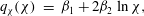 $$\begin{eqnarray}\displaystyle q_{{\it\chi}}({\it\chi}) & = & \displaystyle {\it\beta}_{1}+2{\it\beta}_{2}\ln {\it\chi},\end{eqnarray}$$
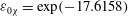 ${\it\varepsilon}_{0{\it\chi}}=\exp (-17.6158)$
,
${\it\varepsilon}_{0{\it\chi}}=\exp (-17.6158)$
,
 ${\it\alpha}_{1}=1.7645$
,
${\it\alpha}_{1}=1.7645$
,
 ${\it\alpha}_{2}=-0.0647$
,
${\it\alpha}_{2}=-0.0647$
,
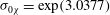 ${\it\sigma}_{0{\it\chi}}=\exp (3.0377)$
,
${\it\sigma}_{0{\it\chi}}=\exp (3.0377)$
,
 ${\it\beta}_{1}=0.3990$
, and
${\it\beta}_{1}=0.3990$
, and
 ${\it\beta}_{2}=-0.0110$
. A sufficient range of the dimensionless fetch
${\it\beta}_{2}=-0.0110$
. A sufficient range of the dimensionless fetch
 ${\it\chi}$
for computation is
${\it\chi}$
for computation is
 $10^{0}{-}10^{6}$
.
$10^{0}{-}10^{6}$
.
Excluding fetch
 ${\it\chi}$
in (5.2a,b
) one has a counterpart of the linear link (2.12) for self-similar solutions of the model (2.2)
${\it\chi}$
in (5.2a,b
) one has a counterpart of the linear link (2.12) for self-similar solutions of the model (2.2)
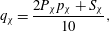 $$\begin{eqnarray}q_{{\it\chi}}=\frac{2P_{{\it\chi}}p_{{\it\chi}}+S_{{\it\chi}}}{10},\end{eqnarray}$$
where
 $$\begin{eqnarray}\displaystyle P_{{\it\chi}}=0.8501,\quad S_{{\it\chi}}=0.9900 & & \displaystyle\end{eqnarray}$$
are remarkably close to the theoretical value of unity. The duration-limited growth functions can be derived from a similar approach using a formal conversion of fetch
 $x$
to time
$x$
to time
 $t$
(see Hwang & Wang Reference Hwang and Wang2004, for details). Trivial algebra leads to a similar relationship between
$t$
(see Hwang & Wang Reference Hwang and Wang2004, for details). Trivial algebra leads to a similar relationship between
 $p_{{\it\tau}}$
and
$p_{{\it\tau}}$
and
 $q_{{\it\tau}}$
(cf. (2.7) and (5.3)), i.e.
$q_{{\it\tau}}$
(cf. (2.7) and (5.3)), i.e.
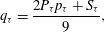 $$\begin{eqnarray}q_{{\it\tau}}=\frac{2P_{{\it\tau}}p_{{\it\tau}}+S_{{\it\tau}}}{9},\end{eqnarray}$$
where the values of coefficients
 $P_{{\it\tau}},S_{{\it\tau}}$
 $$\begin{eqnarray}\displaystyle P_{{\it\tau}}=0.8492,\quad S_{{\it\tau}}=0.9889, & & \displaystyle\end{eqnarray}$$
again, appear to be quite close to the theoretical value of unity. The empirical fits (5.3), (5.5) and their theoretical counterparts (2.7), (2.12) are shown in figure 1.
One can examine the correspondence between the theory and the empirical knowledge by following the notes in the Introduction. After excluding wind speed from (1.3) one can easily obtain ‘empirical’ invariants (1.7):
 $$\begin{eqnarray}{\it\mu}^{4}{\it\nu}^{r_{{\it\tau}}}=\text{const}_{{\it\tau}},\quad {\it\mu}^{4}{\it\nu}^{r_{{\it\chi}}}=\text{const}_{{\it\chi}}\end{eqnarray}$$
in which exponents
 $r_{{\it\tau}},r_{{\it\chi}}$
depend on growth rates
$r_{{\it\tau}},r_{{\it\chi}}$
depend on growth rates
 $p_{{\it\tau}}$
(
$p_{{\it\tau}}$
(
 $p_{{\it\chi}}$
). Generally, these exponents are close to unity as predicted by our theory (see (1.4)) but can vary in a wide range, even being negative for high exponents
$p_{{\it\chi}}$
). Generally, these exponents are close to unity as predicted by our theory (see (1.4)) but can vary in a wide range, even being negative for high exponents
 $p_{{\it\tau}},p_{{\it\chi}}$
.
$p_{{\it\tau}},p_{{\it\chi}}$
.

Figure 4. Dependence of experimental estimate of self-similarity parameter
 ${\it\alpha}_{0}$
: (a) on non-dimensional fetch
${\it\alpha}_{0}$
: (a) on non-dimensional fetch
 ${\it\chi}=xg/U_{10}^{2}$
and duration
${\it\chi}=xg/U_{10}^{2}$
and duration
 ${\it\tau}=tg/U_{10}$
; (b) on non-dimensional frequency of spectral peak
${\it\tau}=tg/U_{10}$
; (b) on non-dimensional frequency of spectral peak
 ${\it\sigma}={\it\omega}_{p}U_{10}/g$
, for a combined collection of duration- and fetch-limited datasets. The dashed line shows the theoretical value
${\it\sigma}={\it\omega}_{p}U_{10}/g$
, for a combined collection of duration- and fetch-limited datasets. The dashed line shows the theoretical value
 ${\it\alpha}_{0(f)}=0.62$
, the solid line is the empirical power-law fit (5.8) by Hwang & Wang (Reference Hwang and Wang2004) for the collection.
${\it\alpha}_{0(f)}=0.62$
, the solid line is the empirical power-law fit (5.8) by Hwang & Wang (Reference Hwang and Wang2004) for the collection.
An alternative formulation of the results allows tracing of the effect of fetch as follows:
 $$\begin{eqnarray}({\it\mu}^{4}{\it\nu})={\it\varepsilon}_{0{\it\chi}}^{2}{\it\sigma}_{0{\it\chi}}^{10}{\it\chi}^{-0.5391+0.0194\ln {\it\chi}}={\it\alpha}_{0}({\it\chi})^{3}.\end{eqnarray}$$
The additional dependence on dimensionless fetch
 ${\it\chi}$
yields a variation of
${\it\chi}$
yields a variation of
 ${\it\alpha}_{0}$
in (5.8) by a factor
${\it\alpha}_{0}$
in (5.8) by a factor
 $2.3833$
when dimensionless fetch varies over a range of five orders of magnitude,
$2.3833$
when dimensionless fetch varies over a range of five orders of magnitude,
 ${\it\chi}=10{-}10^{6}$
. Figure 4 show the results of these field measurements similarly to figure 2 for simulations. The theoretical reference value of
${\it\chi}=10{-}10^{6}$
. Figure 4 show the results of these field measurements similarly to figure 2 for simulations. The theoretical reference value of
 ${\it\alpha}_{0}$
is reasonably consistent with experimental data and with the empirical fitting (5.8) by Hwang & Wang (Reference Hwang and Wang2004). Typically, the duration-limited data show larger scatter, reflecting the departure from ideal duration-limited wave generation conditions as discussed at the beginning of this section.
${\it\alpha}_{0}$
is reasonably consistent with experimental data and with the empirical fitting (5.8) by Hwang & Wang (Reference Hwang and Wang2004). Typically, the duration-limited data show larger scatter, reflecting the departure from ideal duration-limited wave generation conditions as discussed at the beginning of this section.

Figure 5. Data by Sverdrup & Munk (Reference Sverdrup and Munk1947): (a,b) wave height–period dependence with the conventional wind speed scaling; (c,d)
 $\tilde{H}(\tilde{T})$
scaled by fetch (c) or time (d); (e,f) estimates of invariants
$\tilde{H}(\tilde{T})$
scaled by fetch (c) or time (d); (e,f) estimates of invariants
 ${\it\alpha}_{0(f)}$
and
${\it\alpha}_{0(f)}$
and
 ${\it\alpha}_{0(d)}$
. The dotted lines in (a–d) show the Toba (Reference Toba1972) law, and the dashed lines in (e,f) our theoretical values of
${\it\alpha}_{0(d)}$
. The dotted lines in (a–d) show the Toba (Reference Toba1972) law, and the dashed lines in (e,f) our theoretical values of
 ${\it\alpha}_{0(f)}$
and
${\it\alpha}_{0(f)}$
and
 ${\it\alpha}_{0(d)}$
. ID in (e,f) corresponds to records’ ID in tables of Sverdrup & Munk (Reference Sverdrup and Munk1947). (a,c,e) Data of table II for fetch-limited cases; (b,d,f) data of table III for duration-limited cases. Names of observation ship and authors are given in the legends of (a,b).
${\it\alpha}_{0(d)}$
. ID in (e,f) corresponds to records’ ID in tables of Sverdrup & Munk (Reference Sverdrup and Munk1947). (a,c,e) Data of table II for fetch-limited cases; (b,d,f) data of table III for duration-limited cases. Names of observation ship and authors are given in the legends of (a,b).
5.2. Data by Sverdrup & Munk (Reference Sverdrup and Munk1947)
The special attention we pay to the work by Sverdrup & Munk (Reference Sverdrup and Munk1947) is not limited to the historical aspects of wind-wave studies. The theoretical construction of their paper is quite close to our physical approach. Ten years before the formulation of the spectral approach for wind waves Sverdrup & Munk (Reference Sverdrup and Munk1947) showed that ‘the concept of ‘significant waves’ is essential for purpose of forecasting’. They started their theory from the equation for the integral balance of energy (see (47) in Sverdrup & Munk Reference Sverdrup and Munk1947), i.e. the counterpart of the second equation of our model (2.2). The effect of nonlinear interactions has been described by a semi-empirical relationship between two dimensionless parameters: wave steepness and wave age. The experimental data available at that time have been used to specify parameters of their model.
Figure 5 presents the data of tables II and III of appendix II by Sverdrup & Munk (Reference Sverdrup and Munk1947). Only measurements containing full triads of wave height, period and fetch (duration) were taken into account. The upper row shows fetch- (figure 5
a) and duration-limited (figure 5
b) data with the conventional wind speed scaling. There is a rather large scatter of data around Toba’s
 $3/2$
law (dotted line). Strong deviations from Toba’s law are associated with four particular data groups: US Eng. and Cornish for fetch- and Krümmel, Dover for duration-limited observations.
$3/2$
law (dotted line). Strong deviations from Toba’s law are associated with four particular data groups: US Eng. and Cornish for fetch- and Krümmel, Dover for duration-limited observations.
The alternative wind-free scaling plots in figure 5(c,d) also show large deviations from the reference dependences (3.7), (3.8) but the ranges of the corresponding dimensionless values are wider, especially, for the duration-limited case (figure 5 d). Again, we can notice a clear disparity of points associated with the source of data and the method of estimating wave parameters. The data of USS Augusta and Gibson (fetch-limited) and of USS Augusta and Berkeley (duration-limited) show better agreement with theoretical dependence (dotted lines). The wave period in these observations was estimated directly whereas those of Krümmel and Paris have been computed from measurements of wavelength.
The data in figure 5(c,d) cover the same range of dimensionless
 $\tilde{T}$
and
$\tilde{T}$
and
 $\tilde{H}$
as the simulations by Zakharov et al. (Reference Zakharov, Resio and Pushkarev2012) in figure 3. One point of duration-limited data (figure 5
d, Paris) appears below the lower limit of
$\tilde{H}$
as the simulations by Zakharov et al. (Reference Zakharov, Resio and Pushkarev2012) in figure 3. One point of duration-limited data (figure 5
d, Paris) appears below the lower limit of
 $\tilde{T}$
in figure 3(b), i.e. in the range we treated as a saturated wave field (see comments in § 4.2). As the opposite extreme, note the data of Gibson that fit both approaches (Toba’s and the new one) fairly well (cf. figure 5
a,c). Two points of Gibson correspond to very young waves in terms of wind speed scaling (wave age
$\tilde{T}$
in figure 3(b), i.e. in the range we treated as a saturated wave field (see comments in § 4.2). As the opposite extreme, note the data of Gibson that fit both approaches (Toba’s and the new one) fairly well (cf. figure 5
a,c). Two points of Gibson correspond to very young waves in terms of wind speed scaling (wave age
 $C/U_{10}=0.22$
and
$C/U_{10}=0.22$
and
 $C/U_{10}=0.28$
, see figure 5
a). Short fetches (
$C/U_{10}=0.28$
, see figure 5
a). Short fetches (
 $1.3$
and 3.5 km) put these points into the upper right corner of figure 5(c). In terms of the ‘life distance’
$1.3$
and 3.5 km) put these points into the upper right corner of figure 5(c). In terms of the ‘life distance’
 $x/{\it\lambda}$
, these points correspond to approximately
$x/{\it\lambda}$
, these points correspond to approximately
 $152$
and
$152$
and
 $267$
wave periods.
$267$
wave periods.
The bottom row, figure 5(e,f) demonstrates a surprising correspondence of the experimental estimates of the invariant
 ${\it\alpha}_{0}$
to our theoretical values. Again, data of USS Augusta, Gibson and Berkeley give the best fit to
${\it\alpha}_{0}$
to our theoretical values. Again, data of USS Augusta, Gibson and Berkeley give the best fit to
 ${\it\alpha}_{0(d)}=0.7$
and
${\it\alpha}_{0(d)}=0.7$
and
 ${\it\alpha}_{0(f)}=0.62$
. The agreement is considered quite good given the relatively poor quality of these early data sets.
${\it\alpha}_{0(f)}=0.62$
. The agreement is considered quite good given the relatively poor quality of these early data sets.
5.3. Data of the field research facility wave riders
The data of wave riders in a near-shore area look very attractive for illustrating the law (1.4) in terms of the dependence of wave height on wave period (3.8). This simple
 $5/2$
power-law dependence is verified with data available at the website of the Field Research Facility of the US Army Corps of Engineers http://www.frf.usace.army.mil/. A summary of the data is given in table 1. The wave riders collected data for many years; for example, Buoy 630 has been operational since 1997 and Buoy 430 since 2008. The most recent data downloaded for this analysis are dated September 2013. The total number of measurements and the number of data points relevant to the fetch-limited setup are listed in table 1. We have selected records when offshore wind direction was
$5/2$
power-law dependence is verified with data available at the website of the Field Research Facility of the US Army Corps of Engineers http://www.frf.usace.army.mil/. A summary of the data is given in table 1. The wave riders collected data for many years; for example, Buoy 630 has been operational since 1997 and Buoy 430 since 2008. The most recent data downloaded for this analysis are dated September 2013. The total number of measurements and the number of data points relevant to the fetch-limited setup are listed in table 1. We have selected records when offshore wind direction was
 $\pm 30^{\circ }$
from the coast normal. Buoy 200 is sheltered by a cape from the north; this is the closest coastline but there is almost no wind from that direction. Direction
$\pm 30^{\circ }$
from the coast normal. Buoy 200 is sheltered by a cape from the north; this is the closest coastline but there is almost no wind from that direction. Direction
 $280^{\circ }$
has been taken as an alternative reference and the corresponding fetch has been set as three times longer than the one from the closest shoreline.
$280^{\circ }$
has been taken as an alternative reference and the corresponding fetch has been set as three times longer than the one from the closest shoreline.
Table 1. Summary of wave rider data of the Field Research Facility of the US Army Corps of Engineers. Wave direction is reported as the direction from which the waves originate, e.g. waves coming from the west have direction
 $270^{\circ }$
.
$270^{\circ }$
.
Wind from the ocean is dominating in this area and only 0.31 % of total number of data points (938 of 305 261) qualifies as consistent with a fetch-limited setup of wave growth. When presented in dimensionless variables (3.1) these data match the theoretical dependence
 $\tilde{H}(\tilde{T})$
(3.8) fairly well as seen in figure 6. The data of the buoys cover a wide range of dimensionless periods (‘life distances’), similar to figures 2–5 for simulations of wave growth, more recent wave growth data reported in Hwang & Wang (Reference Hwang and Wang2004) and the historical data by Sverdrup & Munk (Reference Sverdrup and Munk1947). A slight overshoot relative to the theoretical dependence can be explained by a systematic underestimating of wave periods. Underestimating of fetch can also contribute to this overshoot when the wave development is slowed down by the coast sheltering effect. The scaling gives a good approximation for the problem of wave growth at relatively small slanting fetches, for our present knowledge up to
$\tilde{H}(\tilde{T})$
(3.8) fairly well as seen in figure 6. The data of the buoys cover a wide range of dimensionless periods (‘life distances’), similar to figures 2–5 for simulations of wave growth, more recent wave growth data reported in Hwang & Wang (Reference Hwang and Wang2004) and the historical data by Sverdrup & Munk (Reference Sverdrup and Munk1947). A slight overshoot relative to the theoretical dependence can be explained by a systematic underestimating of wave periods. Underestimating of fetch can also contribute to this overshoot when the wave development is slowed down by the coast sheltering effect. The scaling gives a good approximation for the problem of wave growth at relatively small slanting fetches, for our present knowledge up to
 $40^{\circ }$
from the coastline normal. At larger angles the wave growth off-shore is accompanied by a complex system of along-shore modes as shown in recent simulations of fetch-limited growth in which the effect of nonlinear wave–wave interactions has been accounted for in full (e.g. Gagnaire-Renou Reference Gagnaire-Renou2009; Zakharov et al.
Reference Zakharov, Resio and Pushkarev2012).
$40^{\circ }$
from the coastline normal. At larger angles the wave growth off-shore is accompanied by a complex system of along-shore modes as shown in recent simulations of fetch-limited growth in which the effect of nonlinear wave–wave interactions has been accounted for in full (e.g. Gagnaire-Renou Reference Gagnaire-Renou2009; Zakharov et al.
Reference Zakharov, Resio and Pushkarev2012).

6. Wind-wave growth observed in laboratory experiments
It is commonly admitted that the dynamics of water waves observed in wind-wave tanks differ dramatically from those of wind waves observed in open seas. Most of the experimental facilities are considered as too short for reaching the full development of wave–wave interactions and for observing the related statistical properties of wind-wave fields. At the same time, a number of laboratory results have been generalized successfully for in situ wave field conditions. Examining a set of wind-wave field data obtained in the laboratory in a wide range of fetch and wind conditions according to the approach developed in this paper may help to clarify, at least partly, the soundness of this viewpoint.
In this section, we consider the results of two experiments made in two different wind-wave tanks. Experiments in the early 1960s by Toba (Reference Toba1961) served as a basis for later works on the famous
 $3/2$
power law by Toba (Reference Toba1972, Reference Toba1973a
,Reference Toba
b
) that links dimensionless wave height and wave period.
$3/2$
power law by Toba (Reference Toba1972, Reference Toba1973a
,Reference Toba
b
) that links dimensionless wave height and wave period.
The observations reported by Caulliez, Makin & Kudryavtsev (Reference Caulliez, Makin and Kudryavtsev2008), Badulin & Caulliez (Reference Badulin and Caulliez2009) and Caulliez (Reference Caulliez2013) were made in the large wind-wave tank in Marseille for various fetches between
 $2$
and 26 m (i.e.
$2$
and 26 m (i.e.
 $2$
,
$2$
,
 $4$
,
$4$
,
 $6$
,
$6$
,
 $9$
,
$9$
,
 $13$
,
$13$
,
 $18$
and 26 m) and
$18$
and 26 m) and
 $10$
wind speeds (values given in the legends of figure 7). Measurements of wind and wave parameters are based on much more advanced technology and methodology, allowing a proper examination of wind-wave development both within the conventional wind scale approach and the above-presented theory.
$10$
wind speeds (values given in the legends of figure 7). Measurements of wind and wave parameters are based on much more advanced technology and methodology, allowing a proper examination of wind-wave development both within the conventional wind scale approach and the above-presented theory.
6.1. Wind speed scaling in experiments by Toba (Reference Toba1961, Reference Toba1972) and Caulliez et al. (Reference Caulliez, Makin and Kudryavtsev2008) and Caulliez (Reference Caulliez2013)
Figure 7(a) shows the classical representation of wind-wave growth in terms of the dimensionless wind-dependent wave parameters
 $H^{\ast }$
and
$H^{\ast }$
and
 $T^{\ast }$
, using the definitions based on wind friction velocity as given by Toba (Reference Toba1972). The whole sets of data obtained respectively by Toba (Reference Toba1972, table 1 therein, filled symbols) and by Caulliez (Reference Caulliez2013, partially given in table 1, open symbols) are displayed. In particular, the Toba and Caulliez data were collected for a number of similar conditions, namely for reference wind speeds between
$T^{\ast }$
, using the definitions based on wind friction velocity as given by Toba (Reference Toba1972). The whole sets of data obtained respectively by Toba (Reference Toba1972, table 1 therein, filled symbols) and by Caulliez (Reference Caulliez2013, partially given in table 1, open symbols) are displayed. In particular, the Toba and Caulliez data were collected for a number of similar conditions, namely for reference wind speeds between
 $5$
and
$5$
and
 $12~\text{m}~\text{s}^{-1}$
and fetches between
$12~\text{m}~\text{s}^{-1}$
and fetches between
 $6$
and 14 m but in facilities of quite different sizes, the water tanks being respectively
$6$
and 14 m but in facilities of quite different sizes, the water tanks being respectively
 $21$
and 40 m long.
$21$
and 40 m long.
In addition, the air layer above Toba’s water tank was just 50 cm in height
 $\times ~75~\text{cm}$
in width and, clearly, the air flow above waves might be affected by the walls. The wind friction velocity was determined from the mean velocity profiles measured at three fetches by means of small cup anemometers while the significant wave height was derived from the mean wave height estimates. When compared to the Marseille data as given in Caulliez et al. (Reference Caulliez, Makin and Kudryavtsev2008) and Caulliez (Reference Caulliez2013), the original data reported by Toba (Reference Toba1972) in figure 7(a) show laboratory waves ‘unrealistically young’ exhibiting abnormally small
$\times ~75~\text{cm}$
in width and, clearly, the air flow above waves might be affected by the walls. The wind friction velocity was determined from the mean velocity profiles measured at three fetches by means of small cup anemometers while the significant wave height was derived from the mean wave height estimates. When compared to the Marseille data as given in Caulliez et al. (Reference Caulliez, Makin and Kudryavtsev2008) and Caulliez (Reference Caulliez2013), the original data reported by Toba (Reference Toba1972) in figure 7(a) show laboratory waves ‘unrealistically young’ exhibiting abnormally small
 $T^{\ast }$
associated with inverse wave age in the range 20–45, i.e. propagating 20–45 times slower than the wind speed estimated at the standard 10 m level (note that for short gravity waves, when neglecting drift current effects on wave propagation,
$T^{\ast }$
associated with inverse wave age in the range 20–45, i.e. propagating 20–45 times slower than the wind speed estimated at the standard 10 m level (note that for short gravity waves, when neglecting drift current effects on wave propagation,
 $T^{\ast }$
corresponds approximately to
$T^{\ast }$
corresponds approximately to
 $2{\rm\pi}$
times the wave age
$2{\rm\pi}$
times the wave age
 $C/u_{\ast }$
). A thorough examination of the data set has shown such very small values of wave age are related to abnormally high values of friction velocity.
$C/u_{\ast }$
). A thorough examination of the data set has shown such very small values of wave age are related to abnormally high values of friction velocity.
The observations reported by Caulliez (Reference Caulliez2013) in the large wind-wave tank in Marseille were made for a wider range of wind speeds and fetches, from 2 m up to 26 m, with an air layer above the water surface of 1.5 m in height and 3.2 m in width. The friction velocity was determined from careful hot-X-wire measurements of the vertical profiles of the turbulent momentum flux in air, a quantity found constant within the whole water surface boundary layer (Caulliez et al.
Reference Caulliez, Makin and Kudryavtsev2008). The significant wave height was estimated as four times the root-mean-square value of the water surface displacements. In this experiment, the inverse wave age varied between
 $4$
and
$4$
and
 $18$
.
$18$
.
In figure 7(a), data sets by both Toba and Caulliez follow quite well the Toba
 $3/2$
power law. However, the Toba data are strictly separated from the Caulliez ones in the range of wave age
$3/2$
power law. However, the Toba data are strictly separated from the Caulliez ones in the range of wave age
 $T^{\ast }$
observed. Additionally, all the Toba data are quite close to the
$T^{\ast }$
observed. Additionally, all the Toba data are quite close to the
 $3/2$
power law while the Caulliez data observed at the shortest fetches, in a range depending on wind speed (up to 26 m at
$3/2$
power law while the Caulliez data observed at the shortest fetches, in a range depending on wind speed (up to 26 m at
 $2.5~\text{m}~\text{s}^{-1}$
to less than 6 m at
$2.5~\text{m}~\text{s}^{-1}$
to less than 6 m at
 $10~\text{m}~\text{s}^{-1}$
) show a transition to a ‘saturated wave field state’, in the words of Toba (Reference Toba1972). These transitional points of the Caulliez data appear as outliers from the ones of Toba collected in the same range of wave age and fetches (e.g. between
$10~\text{m}~\text{s}^{-1}$
) show a transition to a ‘saturated wave field state’, in the words of Toba (Reference Toba1972). These transitional points of the Caulliez data appear as outliers from the ones of Toba collected in the same range of wave age and fetches (e.g. between
 $6$
and 14 m).
$6$
and 14 m).
Therefore, Toba’s data have been re-analyzed by using more realistic values of wind and wave parameters based on the detailed measurements made in the large Marseille wind-wave tank. In brief, new friction velocity values have been derived from drag coefficient estimates obtained in Marseille at the same fetches and reference wind speeds as Toba’s data. Note that these new values are in very good agreement with the
 $u_{\ast }$
values measured by Kawai (Reference Kawai1979) in a wind-wave tank of size comparable to the tank used by Toba (Reference Toba1961) in the experiments analyzed here. In addition, significant wave height has been evaluated from the mean wave height given by Toba (Reference Toba1972) on the basis of the wave height probability distribution observed in Marseille and not from the Rayleigh distribution generally assumed for in situ conditions (see for instance figure 9 in Caulliez et al.
Reference Caulliez, Makin and Kudryavtsev2008). When these new parameters are used for estimating
$u_{\ast }$
values measured by Kawai (Reference Kawai1979) in a wind-wave tank of size comparable to the tank used by Toba (Reference Toba1961) in the experiments analyzed here. In addition, significant wave height has been evaluated from the mean wave height given by Toba (Reference Toba1972) on the basis of the wave height probability distribution observed in Marseille and not from the Rayleigh distribution generally assumed for in situ conditions (see for instance figure 9 in Caulliez et al.
Reference Caulliez, Makin and Kudryavtsev2008). When these new parameters are used for estimating
 $T^{\ast }$
and
$T^{\ast }$
and
 $H^{\ast }$
, it is striking to see in figure 7(b) that both data sets again agree very well but now, in a more realistic way, fall into the same range of wave age
$H^{\ast }$
, it is striking to see in figure 7(b) that both data sets again agree very well but now, in a more realistic way, fall into the same range of wave age
 $T^{\ast }$
. As previously mentioned, they also follow remarkably well the
$T^{\ast }$
. As previously mentioned, they also follow remarkably well the
 $3/2$
power law except for the non-saturated wave fields observed at the shortest fetches.
$3/2$
power law except for the non-saturated wave fields observed at the shortest fetches.

Figure 7. Data of wind-wave tank studies of wave growth by Toba (Reference Toba1972) (filled symbols) and by Caulliez (Reference Caulliez2013) (open symbols) made dimensionless by using the gravity parameter
 $g$
and the conventional friction velocity
$g$
and the conventional friction velocity
 $u^{\ast }=\langle U^{\prime }W^{\prime }\rangle ^{1/2}$
(
$u^{\ast }=\langle U^{\prime }W^{\prime }\rangle ^{1/2}$
(
 $T^{\ast }=gT/u^{\ast }$
and
$T^{\ast }=gT/u^{\ast }$
and
 $H^{\ast }=gH_{s}/{u^{\ast }}^{2}$
). (a) Toba’s data derived from table 1 in Toba (Reference Toba1972); (b) friction velocity values
$H^{\ast }=gH_{s}/{u^{\ast }}^{2}$
). (a) Toba’s data derived from table 1 in Toba (Reference Toba1972); (b) friction velocity values
 $u^{\ast }$
given in Toba (Reference Toba1972) are replaced by estimates at the same reference wind speed and fetch made on the basis of the Caulliez measurements in the large Marseille wind wave tank. Solid line is the Toba (Reference Toba1972)
$u^{\ast }$
given in Toba (Reference Toba1972) are replaced by estimates at the same reference wind speed and fetch made on the basis of the Caulliez measurements in the large Marseille wind wave tank. Solid line is the Toba (Reference Toba1972)
 $3/2$
law.
$3/2$
law.

Figure 8. Data derived from wind-wave tank studies of wave growth by Toba (Reference Toba1972) (filled symbols) and by Caulliez (Reference Caulliez2013) (open symbols) plotted in terms of the new scaling (3.1). Solid line is the Toba (Reference Toba1972)
 $3/2$
law.
$3/2$
law.
6.2. Wind-free scaling in experiments by Toba (Reference Toba1961, Reference Toba1972) and Caulliez (Reference Caulliez2013)
Figure 8 shows the same data sets obtained by Caulliez and Toba but plotted with the new scaling representation (3.1) based on the law of universality (1.4). For Toba’s data in figure 8, the significant wave height has been estimated in the same way as in figure 7(b). The correspondence between the two experimental data sets and the theoretical
 $5/2$
power-law dependence (3.8) looks very good for the well-developed wave fields observed at the largest fetches, but the experimental points of Toba (Reference Toba1972) are located about 1.5 times higher than the theoretical curve given by (3.8). This overshoot may be explained by the use of different methods for estimating the spatial wave period
$5/2$
power-law dependence (3.8) looks very good for the well-developed wave fields observed at the largest fetches, but the experimental points of Toba (Reference Toba1972) are located about 1.5 times higher than the theoretical curve given by (3.8). This overshoot may be explained by the use of different methods for estimating the spatial wave period
 $\tilde{T}$
as given by (2.19) and (3.4).
$\tilde{T}$
as given by (2.19) and (3.4).
For fetch-limited conditions, as seen from (2.19), the dimensionless spatial wave period is a measure of the number of waves propagating over the fetch distance
 $x$
, i.e.
$x$
, i.e.
 $\tilde{T}=(2|\boldsymbol{k}_{p}|x)^{-1/2}$
. In the Toba (Reference Toba1972) experiments based on one-point wave gauge measurements, wave period was first derived from the mean-over-spectrum or dominant peak time scale and the related spatial quantity
$\tilde{T}=(2|\boldsymbol{k}_{p}|x)^{-1/2}$
. In the Toba (Reference Toba1972) experiments based on one-point wave gauge measurements, wave period was first derived from the mean-over-spectrum or dominant peak time scale and the related spatial quantity
 $\tilde{T}$
was estimated by using the linear dispersion relation for gravity waves. Caulliez (Reference Caulliez2013) however measured directly the phase speed
$\tilde{T}$
was estimated by using the linear dispersion relation for gravity waves. Caulliez (Reference Caulliez2013) however measured directly the phase speed
 $C_{p}$
of dominant waves by means of a cross-correlation method between two wave signals recorded by a pair of wave gauges (Dudis Reference Dudis1981). This method enables direct measurement of the velocity of wave propagation accounting for the effect of surface drift current and, for the shortest waves, the effect of surface tension. In the observations reported here, the magnitude of these combined effects varies between 70 % of the linear phase velocity value for small fetches and wind speeds, to 10 % for large fetches and winds. This clearly indicates that the dynamics of wind-wave fields observed in the laboratory are governed not only by the gravity force but also by surface drift and, at the shortest scales, by capillary forces.
$C_{p}$
of dominant waves by means of a cross-correlation method between two wave signals recorded by a pair of wave gauges (Dudis Reference Dudis1981). This method enables direct measurement of the velocity of wave propagation accounting for the effect of surface drift current and, for the shortest waves, the effect of surface tension. In the observations reported here, the magnitude of these combined effects varies between 70 % of the linear phase velocity value for small fetches and wind speeds, to 10 % for large fetches and winds. This clearly indicates that the dynamics of wind-wave fields observed in the laboratory are governed not only by the gravity force but also by surface drift and, at the shortest scales, by capillary forces.
The good agreement observed in figure 8 between the Caulliez (Reference Caulliez2013) data at large fetches and the theoretical curve given by (3.8), in contrast to the Toba (Reference Toba1972) data, validates the use of this experimental method for estimating
 $\tilde{T}$
for wind-wave tank observations. This noticeable fit also supports the appropriateness of the new scaling approach for describing well-developed wind-wave fields observed in laboratory at large fetches.
$\tilde{T}$
for wind-wave tank observations. This noticeable fit also supports the appropriateness of the new scaling approach for describing well-developed wind-wave fields observed in laboratory at large fetches.
Finally, figures 7 and 8 enable us to consider two issues thoroughly: the success of the new approach for wind-wave tank observations and the related relevance of the conventional wind speed scaling under Toba’s law. To support this viewpoint, one can also notice that, in figure 8, the range of dimensionless periods
 $\tilde{T}$
observed at the smallest wind speeds overlaps the data of the Field Research Facility for buoys 190 and 630 located at the minimal distances from the coast, i.e. at 3 and 6 km respectively (see figure 6). The equivalent dimensionless fetch in terms of wavelength – the number of waves
$\tilde{T}$
observed at the smallest wind speeds overlaps the data of the Field Research Facility for buoys 190 and 630 located at the minimal distances from the coast, i.e. at 3 and 6 km respectively (see figure 6). The equivalent dimensionless fetch in terms of wavelength – the number of waves
 ${\it\nu}$
– for the wind-wave tank data can be estimated as
${\it\nu}$
– for the wind-wave tank data can be estimated as
 $50$
to
$50$
to
 $300$
, i.e. values quite close to those obtained by Gibson (
$300$
, i.e. values quite close to those obtained by Gibson (
 $\tilde{T}$
is
$\tilde{T}$
is
 $152$
and
$152$
and
 $266$
at fetches
$266$
at fetches
 $1.3$
and 3.5 km and wind speeds
$1.3$
and 3.5 km and wind speeds
 $16.5$
and
$16.5$
and
 $16~\text{m}~\text{s}^{-1}$
respectively) described in our analysis of the Sverdrup & Munk (Reference Sverdrup and Munk1947) results. Thus, with the new approach one can see that wind waves of lengths higher than roughly 15 cm observed in large water tanks are developed enough to be considered for modelling the nonlinear interactions and statistical properties of the resulting wave field.
$16~\text{m}~\text{s}^{-1}$
respectively) described in our analysis of the Sverdrup & Munk (Reference Sverdrup and Munk1947) results. Thus, with the new approach one can see that wind waves of lengths higher than roughly 15 cm observed in large water tanks are developed enough to be considered for modelling the nonlinear interactions and statistical properties of the resulting wave field.
6.3. Toba’s law and the wind-free approach: similarities and dissimilarities
The data presented here and in the previous sections (see figure 5 for data by Sverdrup & Munk Reference Sverdrup and Munk1947) show quite good correspondence of the observations both with our theoretical dependences and with Toba’s power law, especially for wind-wave tank experiments. It reflects, in a sense, the similarities between the basic physical assumptions of both the purely theoretical model described here and the theoretical–empirical model by Toba (Reference Toba1972). Both models consider physical mechanisms providing a local balance (as emphasized in the title of the paper by Toba Reference Toba1972).
Toba (Reference Toba1972) develops his model using a dimensional analysis, associating the wave energy growth rate with the work of the wave-induced wind stress in the field of wave orbital motions. Assuming that this work is directly controlled by the local air flow (and not by wave parameters), and then is proportional to
 $u^{\ast 3}$
, he derived the so-called
$u^{\ast 3}$
, he derived the so-called
 $3/2$
Toba relationship between the dimensionless wave height and wave period. Note that this law is equivalent to proportionality of the total drift current including the Stokes one (i.e. the averaged value of the orbital velocity) and the friction velocity
$3/2$
Toba relationship between the dimensionless wave height and wave period. Note that this law is equivalent to proportionality of the total drift current including the Stokes one (i.e. the averaged value of the orbital velocity) and the friction velocity
 $u^{\ast }$
. This relation that links the wave steepness to the root-mean-square of the inverse wave age expresses the local equilibrium of the dominant wind-wave field but here the treatment is heuristical rather than theoretically well-grounded.
$u^{\ast }$
. This relation that links the wave steepness to the root-mean-square of the inverse wave age expresses the local equilibrium of the dominant wind-wave field but here the treatment is heuristical rather than theoretically well-grounded.
One of the reviewers pointed out that the Stokes drift current is an essentially nonlinear effect of second order in the wave steepness and, thus, unrelated to viscosity and to friction velocity: it is present in a nonlinear wave field in the absence of wind as well. The Stokes drift current therefore can be easily observed in laboratory flumes where waves are generated mechanically by a wavemaker. In the present use of the terminology (of Stokes drift), we mean a somewhat different contribution to the total drift current that results from the shear stress on the air–water interface due to the presence of wind. Interestingly, in laboratory wind-wave facilities these two different contributions to the drift current at the water surface are often of comparable magnitude.
On the contrary, in the present theoretical model we assume the nonlinear interactions to be dominant compared to the external forcing terms
 $S_{in}$
and
$S_{in}$
and
 $S_{diss}$
and exploit the key features of nonlinear transfer among the random water wave field components explicitly. The remarkable fact is that one can express the corresponding balance of the wave field energy (or momentum, or action) in terms of wave parameters only, without any reference to wind forcing and/or dissipation. However, when examining this model in terms of the dependence of wave height on wave period, this balance gives the Toba
$S_{diss}$
and exploit the key features of nonlinear transfer among the random water wave field components explicitly. The remarkable fact is that one can express the corresponding balance of the wave field energy (or momentum, or action) in terms of wave parameters only, without any reference to wind forcing and/or dissipation. However, when examining this model in terms of the dependence of wave height on wave period, this balance gives the Toba
 $3/2$
law but as an important special case of local wave field equilibrium for which the flux of energy to waves (or the ‘rate of work done by the wind stress to wind waves’ in the words of Toba Reference Toba1972) remains constant. Furthermore, as shown in Gagnaire-Renou et al. (Reference Gagnaire-Renou, Benoit and Badulin2011), the wave energy growth rate can be expressed as a function of
$3/2$
law but as an important special case of local wave field equilibrium for which the flux of energy to waves (or the ‘rate of work done by the wind stress to wind waves’ in the words of Toba Reference Toba1972) remains constant. Furthermore, as shown in Gagnaire-Renou et al. (Reference Gagnaire-Renou, Benoit and Badulin2011), the wave energy growth rate can be expressed as a function of
 $u^{\ast 3}$
. The present model thus leads to expressing the strong assumption made by Toba (Reference Toba1972) as the result of the predominance of nonlinear interactions among the other processes governing the wind-wave field evolution. It also means that, in this case, both models represent very similar physics, but here our model reveals more precisely the governing physical mechanisms.
$u^{\ast 3}$
. The present model thus leads to expressing the strong assumption made by Toba (Reference Toba1972) as the result of the predominance of nonlinear interactions among the other processes governing the wind-wave field evolution. It also means that, in this case, both models represent very similar physics, but here our model reveals more precisely the governing physical mechanisms.
The mathematically consistent analysis of the model (2.2) allows the effect of dominating nonlinearity to be accounted for in a quite ‘flexible’ way as two-parametric families of self-similar solutions (2.6), (2.11) and, thus, a description of energy flux that depends on time or fetch. The ‘freedom’ of these solutions comes from homogeneity properties (2.3), i.e. from arbitrariness of physical scaling of deep-water wave lengths and heights (coefficients
 ${\it\upsilon}$
and
${\it\upsilon}$
and
 ${\it\varrho}$
in (2.3)). It allows the balancing of the dominating nonlinear wave transfer and the total net input (see (2.2b
)) in a wide range of physically relevant wind-wave growth scenarios when energy income depends on time or fetch. On the contrary, the restrictiveness of Toba’s model is inherently associated with the definite physical scale of wind speed. Toba fixes this scale by postulating that ‘the growth of wind waves is predicted by an integration with respect to the fetch and duration’ (Toba Reference Toba1972, p. 18) and, hence, in fact, by freezing a particular scenario of wave development at constant energy growth rate.
${\it\varrho}$
in (2.3)). It allows the balancing of the dominating nonlinear wave transfer and the total net input (see (2.2b
)) in a wide range of physically relevant wind-wave growth scenarios when energy income depends on time or fetch. On the contrary, the restrictiveness of Toba’s model is inherently associated with the definite physical scale of wind speed. Toba fixes this scale by postulating that ‘the growth of wind waves is predicted by an integration with respect to the fetch and duration’ (Toba Reference Toba1972, p. 18) and, hence, in fact, by freezing a particular scenario of wave development at constant energy growth rate.
A divergence of the two approaches is then observed beyond the quite restrictive Toba’s wave growth scenario, i.e. when the energy flux to waves varies with time or fetch. The cases by Hasselmann et al. (Reference Hasselmann, Ross, Müller and Sell1976) and Zakharov & Zaslavsky (Reference Zakharov and Zaslavsky1983) considered above (see also Gagnaire-Renou et al.
Reference Gagnaire-Renou, Benoit and Badulin2011) provide other exponents in the dependence of wave height on frequency. In the context of this problem, the consistency between the ‘wind-based’ model by Toba and our ‘wind-free’ model, especially for wind-wave tank observations (cf. figures 7 and 8) might be the most striking manifestation of the ‘universal’ behaviour of wind–wave coupling occurring in the laboratory when external air and water flow disturbances are minimized. These conditions make the friction velocity
 $u^{\ast }$
a fully representative physical parameter.
$u^{\ast }$
a fully representative physical parameter.
7. Discussion and conclusions
In this paper we revisit a variety of theoretical, numerical and experimental results obtained previously over several decades in order to examine in detail a new theoretical concept of wind-wave growth. This final section aims to show the inner consistency and logic of this reconsideration.
7.1. Theory
The key result of this paper is the invariant (1.4) of wind-wave field growth. The basic assumption of the dominating role of nonlinear wave transfer leads to the property of self-similarity of wind-wave spectra for the reference cases of duration- and fetch-limited wave growth and the power-law dependence of dimensionless wave parameters on fetch and time duration (1.3). In contrast to the traditional power-law fits with four free parameters, the theoretical analysis demonstrates the existence of rigid links between exponents and pre-exponents of (1.3). These universal links then give us the universal form of the invariant (1.4), (cf. (1.7)) with the right-hand-side
 ${\it\alpha}_{0}$
being expressed by cumbersome integral dependences of spectral shape functions (e.g. Hasselmann et al.
Reference Hasselmann, Ross, Müller and Sell1976). We assume
${\it\alpha}_{0}$
being expressed by cumbersome integral dependences of spectral shape functions (e.g. Hasselmann et al.
Reference Hasselmann, Ross, Müller and Sell1976). We assume
 ${\it\alpha}_{0}$
to be constant based on previous experimental and numerical studies that showed spectral shape invariance of growing wind seas. The ultimate result of these theoretical considerations implies a surprising conclusion that appears to contradict the present understanding of wind-wave growth: the invariant (1.4) does not contain wind parameters explicitly. In other words:
${\it\alpha}_{0}$
to be constant based on previous experimental and numerical studies that showed spectral shape invariance of growing wind seas. The ultimate result of these theoretical considerations implies a surprising conclusion that appears to contradict the present understanding of wind-wave growth: the invariant (1.4) does not contain wind parameters explicitly. In other words:
![]()
This wind-free paradigm implies a new scaling of dimensionless wave height and period (3.7), (3.8): the simple time duration or fetch becomes a key physical scale irrespective of the conditions of wind forcing. We show that the new theoretical dependences agree fairly well with conventional theoretical–empirical ones (e.g. Hasselmann et al.
Reference Hasselmann, Ross, Müller and Sell1976; Carter Reference Carter1982). Exclusion of wind speed from these dependences gives exactly exponents
 $9/4,5/2$
and, what is more surprising, provides consistent estimates of basic constants
$9/4,5/2$
and, what is more surprising, provides consistent estimates of basic constants
 ${\it\alpha}_{0(d)},{\it\alpha}_{0(f)}$
(see (3.11)). In particular, the reference to the theoretical–empirical model by Hasselmann et al. (Reference Hasselmann, Ross, Müller and Sell1976) is quite representative. The purely theoretical approach shows that the empirical estimations of the parameters in the JONSWAP spectrum and its specific spectral shape are, in a sense, exhaustive for the analysis: the results are substantiated by much more general physical principles.
${\it\alpha}_{0(d)},{\it\alpha}_{0(f)}$
(see (3.11)). In particular, the reference to the theoretical–empirical model by Hasselmann et al. (Reference Hasselmann, Ross, Müller and Sell1976) is quite representative. The purely theoretical approach shows that the empirical estimations of the parameters in the JONSWAP spectrum and its specific spectral shape are, in a sense, exhaustive for the analysis: the results are substantiated by much more general physical principles.
7.2. Simulations of wind-wave growth
We stress that all the numerical experiments were accomplished almost ten years ago with no reference to our findings in this paper. A series of runs for a duration-limited setup from Badulin et al. (Reference Badulin, Pushkarev, Resio and Zakharov2005, Reference Badulin, Babanin, Resio and Zakharov2007a , Reference Badulin, Babanin, Resio, Zakharov, Borisov, Kozlov, Mamaev and Sokolovskiy2008) taken arbitrarily showed a very good agreement with the results of this new theory.
The recent numerical study of fetch-limited growth by Zakharov et al. (Reference Zakharov, Resio and Pushkarev2012) gives us a broader view of the classic problem of wind-wave growth. We found that the fetch-limited regime is just an intermediate asymptotic stage when wave growth is limited in space. When waves from the coast arrive at the opposite side of the simulation domain the waves continue to grow but according to a duration-limited scenario.
7.3. Field experiments on wind-wave growth
Field studies of wave growth provide the dominant support for the new theory. First, we show that the parameters of the power-law experimental fitting (1.3a−d ) are linked. The theoretical links (2.7), (2.12) reproduce the parameterizations by Hwang & Wang (Reference Hwang and Wang2004) reasonably well: a minor quantitative difference makes the invariant (1.4) weakly dependent on dimensionless fetch (or wave age).
The outcome of our historical review of the brilliant paper by Sverdrup & Munk (Reference Sverdrup and Munk1947) is two-fold. First, we show that the relatively coarse wave observations made during World War II are consistent with our theory. Secondly, we emphasize the parallel between our self-similarity approach and the concept of significant wave height. Both approaches describe the wave field with a minimal number of parameters: significant wave height and peak period, in contrast to the more detailed but much more expensive representation of wave field as an ensemble of a great number of spectral components.
Data from wave riders of the US East Coast were analyzed as an additional justification of these new theoretical outcomes. Wave heights and periods scaled by the new wind-speed-free parameterization show remarkable closeness to the
 $5/2$
law for the fetch-limited case. We expect that more experimental proof of the validity of such an approach can be found in more wave data.
$5/2$
law for the fetch-limited case. We expect that more experimental proof of the validity of such an approach can be found in more wave data.
7.4. Wind-wave tank experiments: beyond the formal validity of the statistical description?
The results obtained from wind-wave tank experiments are found to be well representative. Even if the wind-wave tank experiments are generally considered as too far from wind-sea reality, careful data treatment enables one to show that it is probably not the case. In terms of the new wind-free scaling the results of experiments in the Large Air-Sea Interaction Facility (LASIF) in Marseille fit the theoretical dependences remarkably well. They correspond to high values of dimensionless
 $\tilde{H},\tilde{T}$
, i.e. those obtained at relatively short fetches. As expected, the statistical description used in this work may not apply in this case. At the same time, the range of wave age observed in the wind-wave tank experiments overlaps those observed by the wave riders. This finding affords promising perspectives for modelling sea waves in large wind-wave facilities (Zavadsky, Liberzon & Shemer Reference Zavadsky, Liberzon and Shemer2013).
$\tilde{H},\tilde{T}$
, i.e. those obtained at relatively short fetches. As expected, the statistical description used in this work may not apply in this case. At the same time, the range of wave age observed in the wind-wave tank experiments overlaps those observed by the wave riders. This finding affords promising perspectives for modelling sea waves in large wind-wave facilities (Zavadsky, Liberzon & Shemer Reference Zavadsky, Liberzon and Shemer2013).
7.5. A final remark
Evidently, the invariant (1.4) does not provide a full description of wind-wave field evolution for the classic setups of duration- and fetch-limited growth. Essentially, it shows that the problem can be split into two steps and, in the first step, gives an essential physical constraint that does not contain any parameters of wind forcing. The effect of wind can be accounted for in the next step to get the full description of wave growth in terms of wave height and period as functions of time, fetch and parameters of wind–sea coupling.
Thus, the concise expression (1.4) shows the validity and prospects of an analytical theory of wind-driven seas. To a certain extent, this result breaks a long-lived belief that the description of wind-driven seas must be the subject of extensive experimental studies and costly simulations rather than the result of an elegant physical theory.
Acknowledgements
Sections 2–4 of the paper are supported by Russian Science Foundation N14-22-00174. Other parts of the work are sponsored by the Office of Naval Research (Naval Research Laboratory PE 61153N), ONR grant N000141010991, National Science Foundation N1130450 and the French Centre National d’Etudes Spatiales (TOSCA/SMOS-Ocean project). Authors are thankful for data provided by the Field Research Facility, Field Data Collections and Analysis Branch, US Army Corps of Engineers, Duck, North Carolina. The NRL publication number is NRL/JA/7260-14-0232. The authors are grateful to referees for their constructive and useful suggestions.
Appendix A. Self-similar solutions for growing wind seas
A.1. Duration-limited case
Let us consider the duration-limited case, i.e. a spatially homogeneous case where
 $\partial E/\partial x\equiv \partial E/\partial y\equiv 0$
. Solutions for the conservative kinetic equation (2.2a
) with homogeneity condition (2.3) can be found in the form of incomplete self-similarity (2.6).
$\partial E/\partial x\equiv \partial E/\partial y\equiv 0$
. Solutions for the conservative kinetic equation (2.2a
) with homogeneity condition (2.3) can be found in the form of incomplete self-similarity (2.6).
After substituting (2.6) into (2.2a ) one has
 $$\begin{eqnarray}(p_{{\it\tau}}+4q_{{\it\tau}}){\it\Phi}_{p_{{\it\tau}}}({\bf\xi})+2q_{{\it\tau}}{\bf\xi}\boldsymbol{{\rm\nabla}}_{{\it\xi}}{\it\Phi}_{p_{{\it\tau}}}=a_{{\it\tau}}^{2}b_{{\it\tau}}^{-17/2}{\it\tau}^{R}S_{nl}[{\it\Phi}_{p_{{\it\tau}}}({\it\xi})],\end{eqnarray}$$
where exponent
 $R=2p_{{\it\tau}}-9q_{{\it\tau}}+1$
should be zero to cancel the explicit dependence on time
$R=2p_{{\it\tau}}-9q_{{\it\tau}}+1$
should be zero to cancel the explicit dependence on time
 ${\it\tau}$
and to leave a dependence on self-similar argument
${\it\tau}$
and to leave a dependence on self-similar argument
 ${\bf\xi}$
only. It gives the linear link (2.7) between exponents
${\bf\xi}$
only. It gives the linear link (2.7) between exponents
 $p_{{\it\tau}}$
and
$p_{{\it\tau}}$
and
 $q_{{\it\tau}}$
. An additional link between coefficients
$q_{{\it\tau}}$
. An additional link between coefficients
 $a_{{\it\tau}}$
and
$a_{{\it\tau}}$
and
 $b_{{\it\tau}}$
(2.8) can be introduced by simple re-scaling of dimensionless variables. The total dimensionless energy for solutions (2.6) with (2.8) becomes
$b_{{\it\tau}}$
(2.8) can be introduced by simple re-scaling of dimensionless variables. The total dimensionless energy for solutions (2.6) with (2.8) becomes
 $$\begin{eqnarray}\tilde{E}_{tot}=\int \int _{-\infty }^{+\infty }a_{{\it\tau}}{\it\tau}^{p_{{\it\tau}}+4q_{{\it\tau}}}{\it\Phi}_{p_{{\it\tau}}}({\bf\xi})\,\text{d}\boldsymbol{k}=a_{{\it\tau}}^{9/17}{\it\tau}^{p_{{\it\tau}}}I_{{\it\tau}}\end{eqnarray}$$
where
 $$\begin{eqnarray}I_{{\it\tau}}=\int \int _{-\infty }^{+\infty }{\it\Phi}_{p_{{\it\tau}}}({\bf\xi})\,\text{d}{\bf\xi}.\end{eqnarray}$$
Links (2.7), (2.8) are of key importance for further consideration. First, equation (A 1) for shape function
 ${\it\Phi}_{p_{{\it\tau}}}({\bf\xi})$
with (2.8) depends on exponents
${\it\Phi}_{p_{{\it\tau}}}({\bf\xi})$
with (2.8) depends on exponents
 $p_{{\it\tau}},q_{{\it\tau}}$
but appears to be independent of coefficients
$p_{{\it\tau}},q_{{\it\tau}}$
but appears to be independent of coefficients
 $a_{{\it\tau}},b_{{\it\tau}}$
. Secondly, the self-similar solutions (2.6) with the integral (A 2) depending on two parameters only (say,
$a_{{\it\tau}},b_{{\it\tau}}$
. Secondly, the self-similar solutions (2.6) with the integral (A 2) depending on two parameters only (say,
 $a_{{\it\tau}}$
and
$a_{{\it\tau}}$
and
 $p_{{\it\tau}}$
) are consistent with a power-law dependence of net wave input on time in (2.2b
).
$p_{{\it\tau}}$
) are consistent with a power-law dependence of net wave input on time in (2.2b
).
A characteristic frequency
 ${\it\omega}_{\ast }$
can be introduced in different ways for a given spectral shape function
${\it\omega}_{\ast }$
can be introduced in different ways for a given spectral shape function
 ${\it\Phi}_{p_{{\it\tau}}}({\bf\xi})$
. The mean-over-spectrum frequency is written as follows:
${\it\Phi}_{p_{{\it\tau}}}({\bf\xi})$
. The mean-over-spectrum frequency is written as follows:
 $$\begin{eqnarray}\tilde{{\it\omega}}_{m}=\frac{\displaystyle \int \int _{-\infty }^{+\infty }\tilde{{\it\omega}}{\it\Phi}_{p_{{\it\tau}}}({\bf\xi})\,\text{d}{\bf\xi}}{\displaystyle \int \int _{-\infty }^{+\infty }{\it\Phi}_{p_{{\it\tau}}}({\bf\xi})\,\text{d}{\bf\xi}}=a_{{\it\tau}}^{-2/17}{\it\tau}^{-q_{{\it\tau}}}J_{{\it\tau}}I_{{\it\tau}}^{-1},\end{eqnarray}$$
where
 $$\begin{eqnarray}J_{{\it\tau}}=\int \int _{-\infty }^{+\infty }|{\bf\xi}|{\it\Phi}_{p_{{\it\tau}}}({\bf\xi})\,\text{d}{\bf\xi}.\end{eqnarray}$$
Peak frequency
 $\tilde{{\it\omega}}_{p}$
that corresponds to a maximum of the shape function
$\tilde{{\it\omega}}_{p}$
that corresponds to a maximum of the shape function
 ${\it\Phi}_{p_{{\it\tau}}}({\bf\xi})$
, evidently, has similar dependence on time and parameter
${\it\Phi}_{p_{{\it\tau}}}({\bf\xi})$
, evidently, has similar dependence on time and parameter
 $a_{{\it\tau}}$
 $$\begin{eqnarray}\tilde{{\it\omega}}_{p}=h_{p_{{\it\tau}}}\tilde{{\it\omega}}_{m}=h_{p_{{\it\tau}}}a_{{\it\tau}}^{-2/17}{\it\tau}^{-q_{{\it\tau}}}J_{{\it\tau}}I_{{\it\tau}}^{-1},\end{eqnarray}$$
where the coefficient
 $h_{p_{{\it\tau}}}<1$
for wind-wave spectra: the mean frequency is generally higher than the peak one. Note that this coefficient depends on the exponent
$h_{p_{{\it\tau}}}<1$
for wind-wave spectra: the mean frequency is generally higher than the peak one. Note that this coefficient depends on the exponent
 $p_{{\it\tau}}$
. Below we use the spectral peak frequency
$p_{{\it\tau}}$
. Below we use the spectral peak frequency
 ${\it\omega}_{p}$
unless otherwise stated.
${\it\omega}_{p}$
unless otherwise stated.
While total wave energy (A 2) and characteristic frequency (A 4), (A 6) are power-law functions, the exponents of which are linked by a linear relationship (2.7) one can construct easily a time-independent invariant in the form
 $$\begin{eqnarray}\tilde{E}_{tot}^{s}\tilde{{\it\omega}}_{p}^{y}{\it\tau}=a_{{\it\tau}}^{9s/17-2y/17}{\it\tau}^{sp_{{\it\tau}}-yq_{{\it\tau}}+1}I_{{\it\tau}}^{s-y}J_{{\it\tau}}^{y}h_{{\it\tau}}^{y}\end{eqnarray}$$
by choosing appropriate exponents
 $s$
and
$s$
and
 $y$
. Exponents
$y$
. Exponents
 $s=2$
and
$s=2$
and
 $y=9$
cancel dependence on time
$y=9$
cancel dependence on time
 ${\it\tau}$
in (A 7). One remarkable result is that this choice cancels dependence on parameter
${\it\tau}$
in (A 7). One remarkable result is that this choice cancels dependence on parameter
 $a_{{\it\tau}}$
as well. Condition (2.7) on exponents
$a_{{\it\tau}}$
as well. Condition (2.7) on exponents
 $p_{{\it\tau}}$
and
$p_{{\it\tau}}$
and
 $q_{{\it\tau}}$
gives a time-independent invariant that depends on one parameter only of the family of self-similar solutions (2.6). The invariant (A 7) can be associated with the weakly turbulent law of wind-wave growth by Badulin et al. (Reference Badulin, Babanin, Resio and Zakharov2007a
) in the form of the Kolmogorov relationship between energy and energy flux (total net input) (2.15). Finally, one has the invariant in a remarkably concise and physically transparent form in terms of wave steepness
$q_{{\it\tau}}$
gives a time-independent invariant that depends on one parameter only of the family of self-similar solutions (2.6). The invariant (A 7) can be associated with the weakly turbulent law of wind-wave growth by Badulin et al. (Reference Badulin, Babanin, Resio and Zakharov2007a
) in the form of the Kolmogorov relationship between energy and energy flux (total net input) (2.15). Finally, one has the invariant in a remarkably concise and physically transparent form in terms of wave steepness
 ${\it\mu}$
(1.5) and number of waves
${\it\mu}$
(1.5) and number of waves
 ${\it\nu}$
as defined by (1.6)
${\it\nu}$
as defined by (1.6)
 $$\begin{eqnarray}{\it\mu}^{4}{\it\nu}=I_{{\it\tau}}^{-7}J_{{\it\tau}}^{9}h_{{\it\tau}}^{9}={\it\alpha}_{ss(d)}^{3}p_{{\it\tau}}={\it\alpha}_{0(d)}.\end{eqnarray}$$
Here we use subscript
 $(d)$
for the duration-limited case.
$(d)$
for the duration-limited case.
A.2. Fetch-limited case
Self-similar solutions for a fetch-limited setup can be considered quite similarly to the duration-limited case. Assuming the wave field to be stationary (
 $\partial E/\partial t\equiv 0$
) and growing in increasing
$\partial E/\partial t\equiv 0$
) and growing in increasing
 $x$
one has self-similar solutions in the form (2.11) and condition (2.13) is quite similar to the duration-limited case.
$x$
one has self-similar solutions in the form (2.11) and condition (2.13) is quite similar to the duration-limited case.
For dimensionless energy (cf. (A 2) with (2.13)) one has
 $$\begin{eqnarray}\tilde{E}_{tot}=\int \int _{-\infty }^{+\infty }a_{{\it\chi}}{\it\tau}^{p_{{\it\chi}}+4q_{{\it\chi}}}{\it\Phi}_{p_{{\it\chi}}}({\bf\zeta})\,\text{d}\boldsymbol{k}=a_{{\it\chi}}^{5/9}{\it\chi}^{p_{{\it\chi}}}I_{{\it\chi}},\end{eqnarray}$$
where
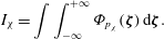 $$\begin{eqnarray}I_{{\it\chi}}=\int \int _{-\infty }^{+\infty }{\it\Phi}_{p_{{\it\chi}}}({\bf\zeta})\,\text{d}{\bf\zeta}.\end{eqnarray}$$
The mean-over-spectrum frequency is written as follows:
 $$\begin{eqnarray}\tilde{{\it\omega}}_{m}=\frac{\displaystyle \int \int _{-\infty }^{+\infty }\tilde{{\it\omega}}{\it\Phi}_{p_{{\it\chi}}}({\bf\zeta})\,\text{d}{\bf\zeta}}{\displaystyle \int \int _{-\infty }^{+\infty }{\it\Phi}_{p_{{\it\chi}}}({\bf\zeta})\,\text{d}{\bf\zeta}}=a_{{\it\chi}}^{-1/9}{\it\chi}^{-q_{{\it\chi}}}J_{{\it\chi}}I_{{\it\chi}}^{-1}\end{eqnarray}$$
and the peak one as
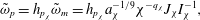 $$\begin{eqnarray}\tilde{{\it\omega}}_{p}=h_{p_{{\it\chi}}}\tilde{{\it\omega}}_{m}=h_{p_{{\it\chi}}}a_{{\it\chi}}^{-1/9}{\it\chi}^{-q_{{\it\chi}}}J_{{\it\chi}}I_{{\it\chi}}^{-1},\end{eqnarray}$$
where
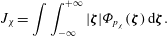 $$\begin{eqnarray}J_{{\it\chi}}=\int \int _{-\infty }^{+\infty }|{\bf\zeta}|{\it\Phi}_{p_{{\it\chi}}}({\bf\zeta})\,\text{d}{\bf\zeta}.\end{eqnarray}$$
The fetch-independent invariant can be derived in the same way as the one for the duration-limited setup (A 7) and related with formulations by Badulin et al. (Reference Badulin, Babanin, Resio and Zakharov2007a ), Gagnaire-Renou et al. (Reference Gagnaire-Renou, Benoit and Badulin2011)
 $$\begin{eqnarray}\tilde{E}_{tot}\tilde{{\it\omega}}_{p}^{4}={\it\alpha}_{ss(f)}\left(\frac{\tilde{{\it\omega}}_{p}^{2}}{2}\frac{\partial \tilde{E}_{tot}}{\partial {\it\chi}}\right)^{1/3}.\end{eqnarray}$$
Finally, one has the invariant in terms of wave steepness
 ${\it\mu}$
(1.5) and number of waves in terms of wavelength
${\it\mu}$
(1.5) and number of waves in terms of wavelength
 $$\begin{eqnarray}\displaystyle {\it\nu}=2\boldsymbol{k}_{p}\boldsymbol{x}, & & \displaystyle\end{eqnarray}$$
which is identical to the duration-limited case
 $$\begin{eqnarray}{\it\mu}^{4}{\it\nu}=I_{{\it\chi}}^{-8}J_{{\it\chi}}^{10}h_{{\it\chi}}^{10}={\it\alpha}_{ss(f)}^{3}p_{{\it\chi}}={\it\alpha}_{0(f)}.\end{eqnarray}$$
The right-hand sides of (A 8), (A 16) are formally different and are determined by self-similar functions
 ${\it\Phi}_{{\it\tau}}({\bf\xi}),{\it\Phi}_{{\it\chi}}({\bf\zeta})$
.
${\it\Phi}_{{\it\tau}}({\bf\xi}),{\it\Phi}_{{\it\chi}}({\bf\zeta})$
.


