2 Model

Here the incompressible flow of a rectangular wing rotating from rest at a fixed, high $\unicode[STIX]{x1D6FC}$ is modelled as a single tilted LEV–TV–TEV–RV loop. The impulse of a thin, 3-D vortex loop can be written in a simple form (Wu, Ma & Zhou Reference Wu, Ma and Zhou2006) as

(2.1) $$\begin{eqnarray}\displaystyle \boldsymbol{I}=\unicode[STIX]{x1D70C}\unicode[STIX]{x1D6E4}\boldsymbol{S}, & & \displaystyle\end{eqnarray}$$

where $\unicode[STIX]{x1D70C}$ is the fluid density, $\unicode[STIX]{x1D6E4}$ is the loop circulation and $\boldsymbol{S}$ is the vector surface spanned by the loop. Once the impulse is known, the net force on the wing in the vertical direction, or lift, can be calculated as

(2.2) $$\begin{eqnarray}\displaystyle & \displaystyle L=L_{in}+\unicode[STIX]{x1D70C}\frac{\text{d}}{\text{d}t}(\unicode[STIX]{x1D6E4}S_{hor}), & \displaystyle\end{eqnarray}$$

where $S_{hor}$ is the projection of the loop area onto the horizontal plane. The second term on the right-hand side is similar to that found in Wu et al. (Reference Wu, Ma and Zhou2006). The two contributions to the net lift are the fluid-inertial force and circulatory force. Here, assuming an infinitely thin flat-plate wing, potential flow theory (Sedov Reference Sedov1965) is used at each wing section to calculate the fluid-inertial lift per unit span. This can be integrated over the entire span to get the net fluid-inertial lift, which for a rectangular, rotating wing is (Percin & van Oudheusden Reference Percin and van Oudheusden2015)

(2.3) $$\begin{eqnarray}\displaystyle & \displaystyle L_{in}=\unicode[STIX]{x03C0}\unicode[STIX]{x1D70C}c^{2}\ddot{\unicode[STIX]{x1D6F7}}\frac{b_{t}^{2}-(b_{t}-b)^{2}}{8}\sin \unicode[STIX]{x1D6FC}\cos \unicode[STIX]{x1D6FC}, & \displaystyle\end{eqnarray}$$

where $\unicode[STIX]{x1D6F7}$ is the wing rotation angle, $\ddot{\unicode[STIX]{x1D6F7}}$ is the angular acceleration, $c$ is the chord, $b$ is the span, $b_{t}$ is the total span, including the root cutout or offset, and $\unicode[STIX]{x1D6FC}$ is the geometric angle of attack (figure 1 a). For the rectangular wings considered here, .

Figure 1(a) also shows an isosurface of the ${\mathcal{Q}}$ -criterion from the  experiments of Carr, DeVoria & Ringuette (Reference Carr, DeVoria and Ringuette2015), to illustrate the real vortex flow for comparison with the model. Here the dimensionless ${\mathcal{Q}}^{\ast }={\mathcal{Q}}c^{2}/(R\unicode[STIX]{x1D6FA})^{2}$ is used, where $R$ is the radius of gyration and $\unicode[STIX]{x1D6FA}$ is the angular speed. A top view of the rotating-wing LEV–TV–TEV–RV loop geometry for the present model is given in figure 1(b). It is a simplification of the experiments and simulations mentioned in § 1, including that of figure 1(a). At the start of rotation, $\unicode[STIX]{x1D6F7}=0$ , the LEV and TEV are collocated at the span-parallel line ( $z$ -axis), which intersects the axis of rotation, making the initial loop area zero. The $z$ -axis moves with the wing as $\unicode[STIX]{x1D6F7}(t)$ increases. It is assumed that there is a single LEV from root to tip that remains attached at this $z$ -axis during wing rotation, discussed further below. The TEV stays fixed at the starting angular position, which is an approximation of the behaviour found by Carr et al. (Reference Carr, DeVoria and Ringuette2015). For the model, the TV and RV formation follow the arcs traversed by the $z$ -axis, at their respective edge locations, starting from $\unicode[STIX]{x1D6F7}=0$ . Therefore, the loop shape is a circular sector growing with $\unicode[STIX]{x1D6F7}(t)$ , minus the root-cutout region.

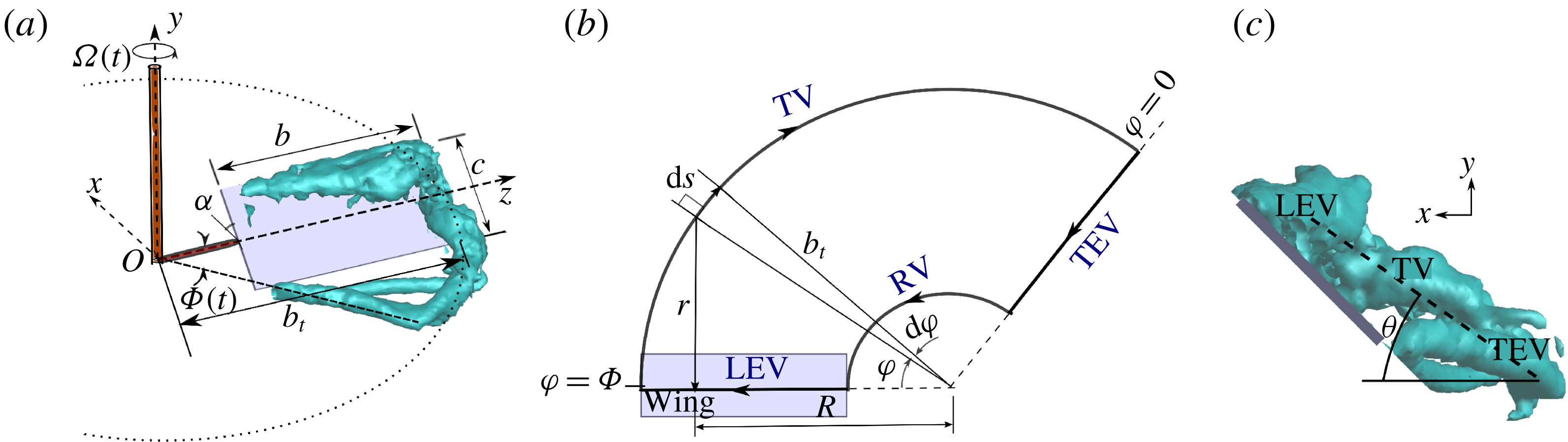
Figure 1. (a) Schematic of the model wing and its motion, including a ${\mathcal{Q}}^{\ast }=6$ isosurface (Carr et al. Reference Carr, DeVoria and Ringuette2015) to illustrate the real vortex loop. (b) Simplified vortex-loop geometry for the model (top view); the loop arrows give the swirl direction. (c) Experimental visualization to conceptually show the model loop angle ( $\unicode[STIX]{x1D703}$ ).

Piston–cylinder vortex-generator experiments have shown that the momentum imparted by the piston to the volume of fluid it displaces is nearly equal to the impulse of the vortex ring (Sullivan et al. Reference Sullivan, Niemela, Hershberger, Bolster and Donnelly2008). Drawing an analogy to the rotating-wing configuration, we assume that the angular impulse of the vortex loop about the axis of wing rotation is equal to the angular momentum of the volume of fluid brought into motion by the wing,

(2.4) $$\begin{eqnarray}\displaystyle m_{f}R^{2}\overline{\unicode[STIX]{x1D6FA}}=\unicode[STIX]{x1D70C}\unicode[STIX]{x1D6E4}S_{ver}R, & & \displaystyle\end{eqnarray}$$

where $m_{f}$ is the mass of this fluid, and the associated volume is approximated as the area swept through by the wing in the horizontal plane, multiplied by the projection of the wing chord onto the vertical plane,

(2.5) $$\begin{eqnarray}\displaystyle & \displaystyle m_{f}=\frac{1}{2}\unicode[STIX]{x1D70C}(c\sin \unicode[STIX]{x1D6FC})(b_{t}^{2}-(b_{t}-b)^{2})\unicode[STIX]{x1D6F7}. & \displaystyle\end{eqnarray}$$

In (2.4), the radius of gyration can be calculated from (2.6) for rectangular plates (Lee, Lua & Lim Reference Lee, Lua and Lim2016a ):

(2.6)

Similar to the mean piston speed in the momentum conservation equation of Sullivan et al. (Reference Sullivan, Niemela, Hershberger, Bolster and Donnelly2008), the running mean of the angular speed, $\overline{\unicode[STIX]{x1D6FA}}(t)$ , is used in (2.4), i.e. at each time the mean is calculated starting from $t=0$ (Gharib, Rambod & Shariff Reference Gharib, Rambod and Shariff1998):

(2.7) $$\begin{eqnarray}\displaystyle & \displaystyle \overline{\unicode[STIX]{x1D6FA}}(t)=\frac{1}{t}\int _{0}^{t}\unicode[STIX]{x1D6FA}(\unicode[STIX]{x1D70F})\,\text{d}\unicode[STIX]{x1D70F}=\frac{\unicode[STIX]{x1D6F7}(t)}{t}. & \displaystyle\end{eqnarray}$$

The $S_{ver}$ in (2.4) is the projection of the vortex loop area onto the vertical plane, derived later.

As mentioned above, it is assumed that the LEV stays attached along the $z$ -axis (or the wing) until the end of the motion. Jardin & Colonius (Reference Jardin and Colonius2018) showed that this is true approximately for a local Rossby number, $Ro$ , of $Ro=z/c<3$ , if the span is long enough to avoid nearby TV effects (see also Lentink & Dickinson Reference Lentink and Dickinson2009; Kruyt et al. Reference Kruyt, van Heijst, Altshuler and Lentink2015). For larger $z/c$ , the LEV moves farther aft and interacts with the trailing tip flow. The LEV evolution depends on $Re$ ,  and $Ro$ (see Bhat et al. (Reference Bhat, Zhao, Sheridan, Hourigan and Thompson2019), who determined that these effects are best isolated using span-based definitions of $Re$ and $Ro$ ), but often exhibits arch-like liftoff outboard and further LEVs forming ahead of the main one (e.g. Jardin, Farcy & David Reference Jardin, Farcy and David2012; Harbig, Sheridan & Thompson Reference Harbig, Sheridan and Thompson2013; Garmann & Visbal Reference Garmann and Visbal2014; Carr et al. Reference Carr, DeVoria and Ringuette2015; Percin & van Oudheusden Reference Percin and van Oudheusden2015; Phillips, Knowles & Bomphrey Reference Phillips, Knowles and Bomphrey2015; Lee et al. Reference Lee, Lua and Lim2016a ; Bhat et al. Reference Bhat, Zhao, Sheridan, Hourigan and Thompson2019). However, the LEV remains close to the wing over much of the span and the overall flow exhibits a growing vortex loop for up to , albeit with complex outboard structures (Garmann & Visbal Reference Garmann and Visbal2014; Carr et al. Reference Carr, DeVoria and Ringuette2015; Jardin & Colonius Reference Jardin and Colonius2018). Therefore, the simplified assumptions of an attached LEV and large-scale, increasing loop structure are reasonable at least for the  values tested in § 3. Taking advantage of this, $S_{hor}$ is calculated as the area traversed by the $z$ -axis in the horizontal plane (figure 1 b):

(2.8) $$\begin{eqnarray}\displaystyle & \displaystyle S_{hor}=\frac{1}{2}(b_{t}^{2}-(b_{t}-b)^{2})\unicode[STIX]{x1D6F7}. & \displaystyle\end{eqnarray}$$

The $S_{hor}$ therefore increases linearly with $\unicode[STIX]{x1D6F7}$ , as also found by Sun & Wu (Reference Sun and Wu2004). For simplicity, the additional wing area is neglected, since including it produces a negligible change in lift. Moreover, placing the LEV at the $z$ -axis reduces the complexity of the Biot–Savart calculation, given below.

As shown in simulations and experiments, the vortex loop is inclined but with a complex, unsteady 3-D geometry (Sun & Wu Reference Sun and Wu2004; Carr et al. Reference Carr, DeVoria and Ringuette2015; Jardin & Colonius Reference Jardin and Colonius2018). This is represented in the model by a single angle $\unicode[STIX]{x1D703}(\unicode[STIX]{x1D6F7})$ with respect to the horizontal (figure 1 c), yielding a planar loop. The $\unicode[STIX]{x1D703}$ is necessary to calculate $S_{ver}$ :

(2.9) $$\begin{eqnarray}\displaystyle & \displaystyle S_{ver}={\textstyle \frac{1}{2}}(b_{t}^{2}-(b_{t}-b)^{2})\unicode[STIX]{x1D6F7}\tan \unicode[STIX]{x1D703}. & \displaystyle\end{eqnarray}$$

From (2.4), $\unicode[STIX]{x1D6E4}$ can then be solved:

(2.10) $$\begin{eqnarray}\displaystyle & \displaystyle \unicode[STIX]{x1D6E4}=\frac{R\overline{\unicode[STIX]{x1D6FA}}c\sin \unicode[STIX]{x1D6FC}}{\tan \unicode[STIX]{x1D703}}. & \displaystyle\end{eqnarray}$$

Lee et al. (Reference Lee, Choi and Kim2015) give a similar expression, but for steady circulation, using a scaling law. The dynamic, 3-D nature of the real vortex loop makes it challenging to model $\unicode[STIX]{x1D703}$ . For simplicity, we conceptualize $\unicode[STIX]{x1D703}$ as being dictated by $\unicode[STIX]{x1D6FC}^{\ast }$ , which is $\unicode[STIX]{x1D6FC}$ scaled by the near-wake flow, and the angle $\unicode[STIX]{x1D6FC}_{i}$ produced by the induced velocity of the loop itself:

(2.11) $$\begin{eqnarray}\displaystyle & \displaystyle \unicode[STIX]{x1D703}(\unicode[STIX]{x1D6F7})=\unicode[STIX]{x1D6FC}^{\ast }-\unicode[STIX]{x1D6FC}_{i}(\unicode[STIX]{x1D6F7}). & \displaystyle\end{eqnarray}$$

The $\unicode[STIX]{x1D6FC}^{\ast }$ term is meant to account for the flow deflection after it passes over the wing. First, we take a reference for the deflection angle to be $\unicode[STIX]{x1D6FC}=\arctan (\sin \unicode[STIX]{x1D6FC}/\cos \unicode[STIX]{x1D6FC})$ , i.e. aligned with the chord line. However, prior work shows that the TE flow does not follow the chord line after it leaves the wing for all $\unicode[STIX]{x1D6FC}$ . For example, at large $\unicode[STIX]{x1D6FC}$ , such as $60^{\circ }$ , the TE flow deflects upwards compared to the chord line (Ozen & Rockwell Reference Ozen and Rockwell2012a ; Garmann & Visbal Reference Garmann and Visbal2014; Li, Dong & Cheng Reference Li, Dong and Cheng2017), implying a reduction of the near-wake downward flow. At smaller $\unicode[STIX]{x1D6FC}$ , e.g.  $15^{\circ }$ , there is evidence that the TE flow is below this line (Jones & Babinsky Reference Jones and Babinsky2011; Li et al. Reference Li, Dong and Cheng2017). To capture this inverse relationship of the near-wake downward flow with $\unicode[STIX]{x1D6FC}$ , the $\sin \unicode[STIX]{x1D6FC}$ is divided by the vertical deflection velocity, $V_{1}$ , from the wing orientation with a scaling factor $K$ to be determined, i.e.  $V_{1}=KR\unicode[STIX]{x1D6FA}\sin \unicode[STIX]{x1D6FC}$ . Also, this can be thought of as accounting for the downwash from the LEV in the near-wake region. Similarly, the $\cos \unicode[STIX]{x1D6FC}$ is divided by the approximate horizontal velocity of the TEV, $V_{2}$ , in the wing-fixed frame, which is estimated to be $R\unicode[STIX]{x1D6FA}$ as discussed above. Effectively, this does not adjust the horizontal flow path, but achieves the desired decrease in the vertical flow deflection with increasing $\unicode[STIX]{x1D6FC}$ for a more physically meaningful $\unicode[STIX]{x1D6FC}^{\ast }$ . Overall, the expression is

(2.12) $$\begin{eqnarray}\displaystyle & \displaystyle \unicode[STIX]{x1D6FC}^{\ast }=\arctan \left(\frac{V_{2}}{V_{1}}\frac{\sin \unicode[STIX]{x1D6FC}}{\cos \unicode[STIX]{x1D6FC}}\right)=\arctan \left(\frac{R\unicode[STIX]{x1D6FA}}{KR\unicode[STIX]{x1D6FA}\sin \unicode[STIX]{x1D6FC}}\frac{\sin \unicode[STIX]{x1D6FC}}{\cos \unicode[STIX]{x1D6FC}}\right)=\arctan \left(\frac{1}{K\cos \unicode[STIX]{x1D6FC}}\right).\quad & \displaystyle\end{eqnarray}$$

The $K$ estimation is motivated by observations from the $\unicode[STIX]{x1D6FC}=45^{\circ }$ ,  rotating-wing data of Carr et al. (Reference Carr, DeVoria and Ringuette2015). Figure 2(a) shows velocity vectors in the rotating frame in an $x$ – $y$ plane at the radius of gyration, for $\unicode[STIX]{x1D6F7}=84^{\circ }$ . In the near wake, the vectors are roughly aligned with the wing chord line, as illustrated by the dashed $45^{\circ }$ reference line in figure 2(a), although there are local spatial variations as expected. This indicates that at $\unicode[STIX]{x1D6FC}=45^{\circ }$ the near-wing wake flow can be approximated as being aligned with the chord, so that $\unicode[STIX]{x1D6FC}^{\ast }\approx \unicode[STIX]{x1D6FC}$ . The ratio of the near-wake downward velocity to the horizontal reference velocity, $v/(R\unicode[STIX]{x1D6FA})$ , is visualized in three dimensions in figure 2(b) using three isosurfaces: $v/(R\unicode[STIX]{x1D6FA})=-1.0$ and $-0.9$ , and ${\mathcal{Q}}^{\ast }=6$ showing the vortex structure. There is a coherent region of magnitude $v/(R\unicode[STIX]{x1D6FA})\sim 1$ in the wake near the radius of gyration. This further suggests that the assumption of $\unicode[STIX]{x1D6FC}^{\ast }\approx \unicode[STIX]{x1D6FC}$ is plausible for $\unicode[STIX]{x1D6FC}=45^{\circ }$ . Wolfinger & Rockwell (Reference Wolfinger and Rockwell2015) also showed regions of magnitude ${\sim}1$ dimensionless downward velocity in the outboard flow of an ,  $\unicode[STIX]{x1D6FC}=45^{\circ }$ wing for high $\unicode[STIX]{x1D6F7}$ and slightly larger $R/c$ . Therefore, the assumption of $\unicode[STIX]{x1D6FC}^{\ast }\approx \unicode[STIX]{x1D6FC}$ at $\unicode[STIX]{x1D6FC}=45^{\circ }$ leads to $K=\sqrt{2}$ . Although $K$ is estimated from observations at only $\unicode[STIX]{x1D6FC}=45^{\circ }$ and , § 3 shows that $\unicode[STIX]{x1D6FC}^{\ast }$ and $\unicode[STIX]{x1D6FC}_{i}$ yield a $\unicode[STIX]{x1D703}$ that allows the model to capture the correct lift trend with  $\unicode[STIX]{x1D6FC}$ .

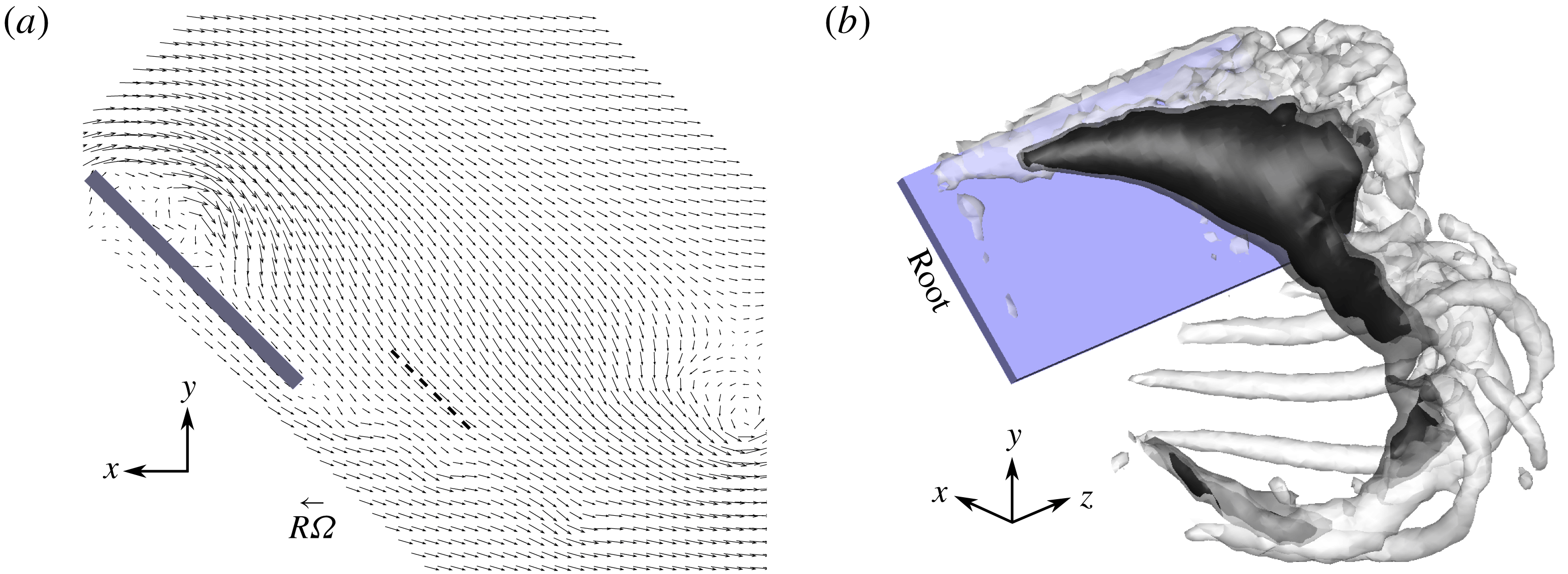
Figure 2. Experimental results from Carr et al. (Reference Carr, DeVoria and Ringuette2015) for ,  $\unicode[STIX]{x1D6FC}=45^{\circ }$ and $\unicode[STIX]{x1D6F7}=84^{\circ }$ motivating $\unicode[STIX]{x1D6FC}^{\ast }$ . (a) Wing-fixed $x$ – $y$ plane velocity vectors at $R$ along the wing span (every other vector is given); a dashed $45^{\circ }$ line is in the near wake for reference. (b) Isosurfaces showing magnitudes of downward velocity and the vortex loop: nested black and translucent grey indicate $v/(R\unicode[STIX]{x1D6FA})=-1.0$ and $-0.9$ , respectively; translucent white is  ${\mathcal{Q}}^{\ast }=6$ .

The induced angle $\unicode[STIX]{x1D6FC}_{i}$ is given by

(2.13) $$\begin{eqnarray}\displaystyle & \displaystyle \tan \unicode[STIX]{x1D6FC}_{i}=\left|\frac{v_{i}}{U_{hor}}\right|=\frac{\unicode[STIX]{x1D6E4}A}{\left|R\overline{\unicode[STIX]{x1D6FA}}-\unicode[STIX]{x1D6E4}A\tan \unicode[STIX]{x1D703}\right|}\approx \frac{\unicode[STIX]{x1D6E4}A}{R\overline{\unicode[STIX]{x1D6FA}}}. & \displaystyle\end{eqnarray}$$

Here $v_{i}$ is the downward induced velocity, $U_{hor}$ is the net horizontal velocity at $R$ from the wing motion and induced by the loop, and $\unicode[STIX]{x1D6E4}A$ is the induced velocity of the horizontally projected loop itself; $A$ is what remains after $\unicode[STIX]{x1D6E4}$ is factored out of the Biot–Savart calculation. The denominator $|R\overline{\unicode[STIX]{x1D6FA}}-\unicode[STIX]{x1D6E4}A\tan \unicode[STIX]{x1D703}|$ can be approximated as $R\overline{\unicode[STIX]{x1D6FA}}$ , since $R\overline{\unicode[STIX]{x1D6FA}}\gg \unicode[STIX]{x1D6E4}A\tan \unicode[STIX]{x1D703}$ .

The $A$ is evaluated on the $z$ -axis at $R$ using the Biot–Savart law at each instant in time ( $\unicode[STIX]{x1D6E4}$ is assumed constant along the loop):

(2.14) $$\begin{eqnarray}\displaystyle & \displaystyle \unicode[STIX]{x1D6E4}\boldsymbol{A}=\frac{\unicode[STIX]{x1D6E4}}{4\unicode[STIX]{x03C0}}\int _{loop}\frac{\text{d}\boldsymbol{s}\times \boldsymbol{r}}{|\boldsymbol{r}|^{3}}, & \displaystyle\end{eqnarray}$$

where $\text{d}\boldsymbol{s}$ is a differential length element along the loop, and $\boldsymbol{r}$ is the position vector from the loop to the point $R$ . This calculation is done for the TV, RV and TEV loop segments, and for illustration figure 1(b) gives the parameters for the TV contribution. The reference position $R$ is taken for $U_{hor}$ and the $A$ calculation, since it has been shown to be the most appropriate wing length scale when non-dimensionalizing and comparing flapping-wing data (Lee et al. Reference Lee, Lua and Lim2016a ). The magnitude $A$ is

(2.15) $$\begin{eqnarray}\displaystyle A=A_{RV}+A_{TV}+A_{TEV}, & & \displaystyle\end{eqnarray}$$

where

(2.16) $$\begin{eqnarray}\displaystyle & \displaystyle A_{RV}=\left|\frac{1}{4\unicode[STIX]{x03C0}}\int _{0}^{\unicode[STIX]{x1D6F7}(t)}(b_{t}-b)\frac{(b_{t}-b)-R\cos \unicode[STIX]{x1D711}}{(R^{2}+(b_{t}-b)^{2}-2R(b_{t}-b)\cos \unicode[STIX]{x1D711})^{3/2}}\,\text{d}\unicode[STIX]{x1D711}\right|, & \displaystyle\end{eqnarray}$$

(2.17) $$\begin{eqnarray}\displaystyle & \displaystyle A_{TV}=\left|\frac{1}{4\unicode[STIX]{x03C0}}\int _{0}^{\unicode[STIX]{x1D6F7}(t)}b_{t}\frac{b_{t}-R\cos \unicode[STIX]{x1D711}}{(R^{2}+b_{t}^{2}-2Rb_{t}\cos \unicode[STIX]{x1D711})^{3/2}}\,\text{d}\unicode[STIX]{x1D711}\right|, & \displaystyle\end{eqnarray}$$

(2.18) $$\begin{eqnarray}\displaystyle & \displaystyle A_{TEV}=\left|\frac{1}{4\unicode[STIX]{x03C0}}\int _{0}^{b}\frac{R\sin \unicode[STIX]{x1D6F7}}{(R^{2}+(b_{t}-\unicode[STIX]{x1D6FD})^{2}-2R(b_{t}-\unicode[STIX]{x1D6FD})\cos \unicode[STIX]{x1D6F7})^{3/2}}\,\text{d}\unicode[STIX]{x1D6FD}\right|. & \displaystyle\end{eqnarray}$$

The modulus is used so the result is consistent with the actual integration path direction. The integrals are of the elliptic form, and therefore can be evaluated analytically. However, in § 3, integrals and derivatives are calculated numerically (trapezoidal rule and second-order least-squares differentiation, respectively) for convenience.

Early in the motion, $A_{TEV}$ (2.18) has a very high value because of the proximity of the LEV to the TEV. However, afterwards, $A_{TEV}$ is very small compared to $A_{TV}$ . Therefore, equation (2.15) is approximated as

(2.19) $$\begin{eqnarray}\displaystyle A=A_{RV}+A_{TV}. & & \displaystyle\end{eqnarray}$$

Then, substituting (2.10), (2.12), (2.13) and (2.19) into (2.11) gives

(2.20) $$\begin{eqnarray}\displaystyle & \displaystyle \sqrt{2}\cos \unicode[STIX]{x1D6FC}\tan ^{2}\unicode[STIX]{x1D703}+(Ac\sin \unicode[STIX]{x1D6FC}-1)\tan \unicode[STIX]{x1D703}+\sqrt{2}Ac\sin \unicode[STIX]{x1D6FC}\cos \unicode[STIX]{x1D6FC}=0. & \displaystyle\end{eqnarray}$$

The root of (2.20) that is physically meaningful is

(2.21) $$\begin{eqnarray}\displaystyle & \displaystyle \tan \unicode[STIX]{x1D703}=\frac{1}{2\sqrt{2}\cos \unicode[STIX]{x1D6FC}}\left[-(Ac\sin \unicode[STIX]{x1D6FC}-1)+\sqrt{(Ac\sin \unicode[STIX]{x1D6FC}-1)^{2}-8Ac\sin \unicode[STIX]{x1D6FC}\cos ^{2}\unicode[STIX]{x1D6FC}}\right].\quad & \displaystyle\end{eqnarray}$$

Later in the motion, for high $\unicode[STIX]{x1D6F7}$ such as $200^{\circ }$ (depending on the wing geometry and kinematics), the root fails and so $\text{d}\unicode[STIX]{x1D703}/\text{d}t$ is frozen thereafter. Once $\unicode[STIX]{x1D703}$ is known, $\unicode[STIX]{x1D6E4}$ is calculated using (2.10). Finally, the $\unicode[STIX]{x1D6E4}$ , $S_{hor}$ (2.8) and $L_{in}$ (2.3) are substituted into (2.2) to compute the time-varying lift. The time average of the $\unicode[STIX]{x1D70C}\,\text{d}(\unicode[STIX]{x1D6E4}S_{hor})/\text{d}t$ term of (2.2) yields a similar expression to that of Jiao et al. (Reference Jiao, Zhao, Shang and Sun2018) for the cycle-averaged thrust of a flapping wing (plunging and twisting) with no root gap. It should be further noted that the current model only requires the wing geometry and kinematics as inputs.

Additionally, a steady-state lift expression is developed from (2.2). Using (2.10) and (2.8), the circulatory lift component, $L_{circ}$ , can be written as

(2.22) $$\begin{eqnarray}\displaystyle L_{circ} & = & \displaystyle \displaystyle \unicode[STIX]{x1D70C}\frac{\text{d}}{\text{d}t}(\unicode[STIX]{x1D6E4}S_{hor})\nonumber\\ \displaystyle & = & \displaystyle \displaystyle \frac{1}{2}R\unicode[STIX]{x1D70C}c\sin \unicode[STIX]{x1D6FC}(b_{t}^{2}-(b_{t}-b)^{2})\left[\frac{2\unicode[STIX]{x1D6F7}\,\text{d}\unicode[STIX]{x1D6F7}/\text{d}t}{t\tan \unicode[STIX]{x1D703}}-\frac{\unicode[STIX]{x1D6F7}^{2}}{t^{2}\tan \unicode[STIX]{x1D703}}-\frac{\unicode[STIX]{x1D6F7}^{2}\,\text{d}\unicode[STIX]{x1D703}/\text{d}t}{t\sin ^{2}\unicode[STIX]{x1D703}}\right].\end{eqnarray}$$

At steady state, $\text{d}\unicode[STIX]{x1D6F7}/\text{d}t$ and $\unicode[STIX]{x1D6F7}/t$ can be individually equated to $\unicode[STIX]{x1D6FA}_{f}$ , where $\unicode[STIX]{x1D6FA}_{f}$ is the final steady angular speed, and $\text{d}\unicode[STIX]{x1D703}/\text{d}t=0$ . The steady-state value for $\tan \unicode[STIX]{x1D703}$ requires the steady-state value of $A$ , which can be determined by assuming the TV and RV to be semi-infinite in length, with circulation $\unicode[STIX]{x1D6E4}$ . The corresponding induced velocity due to both vortices is still calculated at $R$ , giving $A_{ss}$ as

(2.23) $$\begin{eqnarray}\displaystyle & \displaystyle A_{ss}=\frac{1}{4\unicode[STIX]{x03C0}}\left[\frac{1}{b_{t}-R}+\frac{1}{R-(b_{t}-b)}\right], & \displaystyle\end{eqnarray}$$

where the first and second terms on the right-hand side are due to the TV and RV, respectively. At steady state, $\tan \unicode[STIX]{x1D703}$ becomes

(2.24) $$\begin{eqnarray}\displaystyle & \displaystyle \tan \unicode[STIX]{x1D703}_{ss}=\frac{1}{2\sqrt{2}\cos \unicode[STIX]{x1D6FC}}\left[-(A_{ss}c\sin \unicode[STIX]{x1D6FC}-1)+\sqrt{(A_{ss}c\sin \unicode[STIX]{x1D6FC}-1)^{2}-8A_{ss}c\sin \unicode[STIX]{x1D6FC}\cos ^{2}\unicode[STIX]{x1D6FC}}\right]. & \displaystyle \nonumber\\ \displaystyle & & \displaystyle\end{eqnarray}$$

Finally, the steady-state values are substituted into (2.22), and $L_{circ}$ is non-dimensionalized by $1/2\unicode[STIX]{x1D70C}U_{R,f}^{2}bc$ to get the steady-state lift coefficient, $C_{L,ss}$ , where $U_{R,f}$ is the final azimuthal velocity at $R$ :

(2.25) $$\begin{eqnarray}\displaystyle & \displaystyle C_{L,ss}=\frac{(2b_{t}-b)\sin \unicode[STIX]{x1D6FC}}{R\tan \unicode[STIX]{x1D703}_{ss}}. & \displaystyle\end{eqnarray}$$

3 Model validation and discussion

We consider six different experimental cases to validate the model, namely , 3 and 4 from Carr et al. (Reference Carr, DeVoria and Ringuette2015), here called UB2, UB3 and UB4, respectively, and  with slower accelerations and varying root cutouts from Manar et al. (Reference Manar, Mancini, Mayo and Jones2016) (UMD-fast) and Percin & van Oudheusden (Reference Percin and van Oudheusden2015) (TUD). We also compare the model with the more gradual acceleration experiment of Manar et al. (Reference Manar, Mancini, Mayo and Jones2016), called UMD-slow. Additionally, we test it against the computational simulation of Phillips, Nakata & Bomphrey (found in Jones et al. Reference Jones, Manar, Phillips, Nakata, Bomphrey, Ringuette, Percin, van Oudheusden and Palmer2016) with a motion profile and geometric parameters matching those of UMD-slow, and that of Garmann & Visbal (Reference Garmann and Visbal2014), here referred to as RVC and AFRL, respectively. The motion for the AFRL case is very gradual in the beginning, and we consider the start of the motion for the model at $\unicode[STIX]{x1D6F7}\approx 1^{\circ }$ . All unsteady cases tested have $\unicode[STIX]{x1D6FC}=45^{\circ }$ , except for AFRL with $\unicode[STIX]{x1D6FC}=60^{\circ }$ . Further, steady-state model results are compared with the experiments of Dickinson, Lehmann & Sane (Reference Dickinson, Lehmann and Sane1999) for various  $\unicode[STIX]{x1D6FC}$ .

Table 1. Cases for model validation.

Figure 3(a) gives the motion profiles for all unsteady cases, and table 1 provides their specific parameters. The force data were extracted from plots in the references and interpolated to a discrete time scale for all cases except the Carr et al. (Reference Carr, DeVoria and Ringuette2015) results, which were directly available. The motion profiles were generated from the equations used in the references. Figure 3(b) shows how the model loop angle $\unicode[STIX]{x1D703}$ varies with $\unicode[STIX]{x1D6F7}$ for all cases. The $\unicode[STIX]{x1D703}$ starts from a value equal to $\unicode[STIX]{x1D6FC}^{\ast }$ , then decreases rapidly and finally becomes nearly constant. All  cases have comparable loop angles for the same  $\unicode[STIX]{x1D6FC}$ .

Figure 3. (a) Motion profiles; UB2, UB3 and UB4 overlap. (b) Loop angle variation.

Figure 4. Comparison of the lift coefficient from the $\unicode[STIX]{x1D6FC}=45^{\circ }$ experimental/numerical cases (solid lines) and the model (dashed lines): (a)  and (b) .

The lift coefficients, $C_{L}=2L/\unicode[STIX]{x1D70C}U_{R,f}^{2}bc$ , for all  and $\unicode[STIX]{x1D6FC}=45^{\circ }$ cases are shown in figure 4(a) and those for the different  tests of Carr et al. (Reference Carr, DeVoria and Ringuette2015) are given in figure 4(b). Figure 5(a) presents the $C_{L}$ comparison for $\unicode[STIX]{x1D6FC}=60^{\circ }$ . The model reasonably predicts $C_{L}$ within 18 % of the experimental results during the wing’s steady motion, except for TUD and UB2, which have maximum errors below 27 %. It is not always effective at capturing the startup-acceleration peak, and the deviation is more than 20 % of the experimental results. However, it gives a reasonable estimate (within 12 % error) of the peak when compared with the numerical simulations. The model’s non-circulatory force component starts to decrease from the peak value before the experimental $C_{L}$ drops for all cases, possibly because of force-signal filtering and also in the experiment the fluid’s inertia continues to exert force past the instant the wing acceleration ceases (Galler et al. Reference Galler, Weymouth and Rival2019).

Figure 5. (a) Unsteady $C_{L}$ versus  and $\unicode[STIX]{x1D6FC}=60^{\circ }$ . (b) Steady-state $C_{L}$ versus $\unicode[STIX]{x1D6FC}$ : .

The model force could be affected at some time instants by the simplifications. For example, a single loop angle $\unicode[STIX]{x1D703}$ is used to represent the orientation of the complex 3-D loop structure; this could incur some error. Also, in determining $\unicode[STIX]{x1D6FC}^{\ast }$ , the tangent of the geometric $\unicode[STIX]{x1D6FC}$ is scaled by the ratio of vertical and horizontal velocities at $R$ , estimated based on observations from experiments/simulations in the near-wake region. Perhaps this could be improved in the future with the knowledge of a detailed analysis of the flow behaviour in this region for varying $\unicode[STIX]{x1D6FC}$ . Further, there is a range of $\unicode[STIX]{x1D6F7}$ between the occurrence of high and low $A_{TEV}$ values for which the TEV is not too close (spatially) to the LEV to make $A_{TEV}$ go to infinity, nor too far for $A_{TEV}$ to be insignificant compared to $A_{TV}$ (see § 2); $A_{TEV}$ significantly contributes to $A$ in this region. Additionally, the presence of split or multiple outboard LEVs in the real high- $Re$ flows, filtering of the experimental data, and set-up constraints such as mounting hardware are not captured by the model.

Table 2. Model error based on mean $C_{L}$ .

Overall, the model may also deviate from the experiments and simulations for the following reasons. First is the assumption that the impulse of the loop is equal to that imparted to the volume of fluid swept by the wing. Sullivan et al. (Reference Sullivan, Niemela, Hershberger, Bolster and Donnelly2008) presented the ratio of impulses measured in an experiment to those calculated from their piston–cylinder model, which uses the same assumption. The impulse is over- or underpredicted up to 10 % for the cases considered (cf. their table 8). Second, the vortex loop area is modelled here as the sector area traversed by the wing. This is a good assumption but they are not exactly equal. Despite these drawbacks, for the UB3, UB4, UMD-fast, RVC and AFRL cases, the error is within 10 % for most of the $\unicode[STIX]{x1D6F7}$ range shown. Also, we calculate the error based on the mean $C_{L}$ taken over $\unicode[STIX]{x1D6F7}$ up to $250^{\circ }$ for each case, as given in table 2. The deviation is within 20 % for all cases, and for some it is below 10 %.

Further, the trends of the model $C_{L}$ show good agreement with those of the experiments and simulations. In all cases, $C_{L}$ increases with a shallow slope even after the wing stops accelerating (figure 4 a and 4 b) for both the model and benchmark cases. This produces a broad local maximum in some of the experimental and numerical $C_{L}$ curves, whereas in others and all the model estimations, the $C_{L}$ simply levels off.

Figure 6. (a) Inertial and circulatory lift coefficients (dashed and solid lines, respectively) for the ,  $\unicode[STIX]{x1D6FC}=45^{\circ }$ cases. (b) Loop circulation for all cases.

Table 3. Comparison of dimensionless $Ac$ and $A_{ss}c$ for cases with various  and $Ro$ .

Figure 5(b) gives the behaviour of the model with $\unicode[STIX]{x1D6FC}$ , comparing the average $C_{L}$ of the unsteady model over $\unicode[STIX]{x1D6F7}=150^{\circ }{-}250^{\circ }$ , and the steady-state form (2.25), to the quasi-steady measurements of Dickinson et al. (Reference Dickinson, Lehmann and Sane1999) for $\unicode[STIX]{x1D6FC}=0^{\circ }{-}90^{\circ }$ . To calculate the $C_{L,ss}$ (2.25), the unsteady $A$ was simplified for long-time behaviour by assuming semi-infinite TV and RV to obtain $A_{ss}$ (cf. § 2). The dimensionless $A_{ss}c$ estimate is very close to the unsteady counterpart in the steady state, as shown for some cases with various  and $Ro=R/c$ in table 3. Dickinson et al. (Reference Dickinson, Lehmann and Sane1999) measured the lift for a robotic fruit-fly wing rotating from rest in a liquid-filled tank. For both the unsteady and steady models, to compare with the experiment we use a rectangular geometry but match their wing area,  and $Ro=2.35$ ; the unsteady model employs the UB2 velocity profile. Figure 5(b) shows excellent agreement between the unsteady- and steady-state forms of the model, and these compare well with the quasi-steady measurements. Together with figures 4 and 5(a), this demonstrates that the model can predict the proper trends with $\unicode[STIX]{x1D6FC}$ . At first the steady-state $C_{L}$ increases with $\unicode[STIX]{x1D6FC}$ , then after approximately $\unicode[STIX]{x1D6FC}=45^{\circ }$ , it decreases to zero at $\unicode[STIX]{x1D6FC}=90^{\circ }$ (figure 5 b).

In figure 6(a), the model inertial and circulatory force components are given for the ,  $\unicode[STIX]{x1D6FC}=45^{\circ }$ cases. In the steady-motion portion, eventually the circulatory forces become very close despite the differences in motion profiles. Figure 6(b) shows the dimensionless vortex loop circulation; $b$ is used in scaling it to represent the loop size. The circulation initially increases with $\unicode[STIX]{x1D6F7}$ ; then its growth substantially reduces after wing acceleration ceases. As given by (2.10), this behaviour is governed by $\overline{\unicode[STIX]{x1D6FA}}(t)$ and $\unicode[STIX]{x1D703}$ , leading to the slowing growth as they level off. The trend of the loop circulation resembles that of the total circulation produced at the LE in the Carr et al. (Reference Carr, DeVoria and Ringuette2015) experiments.