2.1 Dynamical model

For the sake of generality in the derivation of the proposed observation optimization procedure, we consider a dynamical model under the generic form

(2.1) $$\begin{eqnarray}\frac{\unicode[STIX]{x2202}q}{\unicode[STIX]{x2202}t}=f(q,\unicode[STIX]{x1D6FD}),\end{eqnarray}$$

where $q$ refers to the model variables, here a flow field, which are defined for a spatial domain $\unicode[STIX]{x1D6FA}$ of any dimension (typically one to three) and a time interval $[0,T]$ . $q$ belongs to the model space denoted by ${\mathcal{M}}$ whose scalar product is defined by

(2.2) $$\begin{eqnarray}\langle q,p\rangle _{{\mathcal{M}}}=\int _{0}^{T}\int _{\unicode[STIX]{x1D6FA}}q(x,t)p(x,t)\,\text{d}x\,\text{d}t\quad \forall q,p\in {\mathcal{M}}.\end{eqnarray}$$

The associated norm is given by $\Vert q\Vert _{{\mathcal{M}}}=\sqrt{\langle q,q\rangle _{{\mathcal{M}}}}\;\forall q\in {\mathcal{M}}$ . Equation (2.1) also involves the nonlinear operator $f$ , which corresponds here to the Navier–Stokes equations, and the vector $\unicode[STIX]{x1D6FD}$ belonging to the parameter space denoted by ${\mathcal{P}}$ . $\unicode[STIX]{x1D6FD}$ may refer to parameters of the dynamical model, boundary conditions, or shape design parameters. In the present study, $\unicode[STIX]{x1D6FD}$ refers to the rotational speed of the cylinder. Given (2.1), the solution $q$ is uniquely specified by the initial condition $q_{0}$ ( $q_{0}(x)=q(x,0)\;\forall x\in \unicode[STIX]{x1D6FA}$ ) and the parameters $\unicode[STIX]{x1D6FD}$ . Before proceeding further, let us introduce a few notations. Given an operator $g$ from vector space ${\mathcal{A}}$ to ${\mathcal{B}}$ , the Gâteaux derivative of $g$ at $a$ in the direction $c$ , with both $a$ and $c$ in ${\mathcal{A}}$ , is denoted by

(2.3) $$\begin{eqnarray}\left.\frac{\unicode[STIX]{x2202}g}{\unicode[STIX]{x2202}a}\right|_{a}(c)=\lim _{\unicode[STIX]{x1D716}\rightarrow 0}\frac{\text{d}}{\text{d}\unicode[STIX]{x1D716}}g(a+\unicode[STIX]{x1D716}c).\end{eqnarray}$$

In the case where $g$ is a functional ( ${\mathcal{B}}=\mathbb{R}$ ), the Gâteaux derivative defined in (2.3) may be related to the Fréchet derivative (referred to as gradient in the following) $\unicode[STIX]{x2202}g/\unicode[STIX]{x2202}a$ at $a$ according to

(2.4) $$\begin{eqnarray}\left.\frac{\unicode[STIX]{x2202}g}{\unicode[STIX]{x2202}a}\right|_{a}(c)=\left\langle \frac{\unicode[STIX]{x2202}g}{\unicode[STIX]{x2202}a}(a),c\right\rangle _{{\mathcal{A}}}.\end{eqnarray}$$

If $g$ is a linear operator, one can define the adjoint operator $g^{\ast }$ according to

(2.5) $$\begin{eqnarray}\langle g(a),b\rangle _{{\mathcal{B}}}=\langle a,g^{\ast }(b)\rangle _{{\mathcal{A}}}\quad \forall a\in {\mathcal{A}},\,\forall b\in {\mathcal{B}}.\end{eqnarray}$$

2.2 Sensitivity of observations

We now examine observations of the state $q$ and their sensitivity with respect to a change in the initial condition $q_{0}$ or the parameters $\unicode[STIX]{x1D6FD}$ . More precisely, we consider a response $R$ of the model defined as the norm of the observations of the state vector  $q$

(2.6) $$\begin{eqnarray}R={\textstyle \frac{1}{2}}\Vert h(q,\unicode[STIX]{x1D706})\Vert _{{\mathcal{O}}}^{2},\end{eqnarray}$$

where $h$ is the observation operator that maps the model space ${\mathcal{M}}$ to the observation space ${\mathcal{O}}$ . It may be worth noting that the scalar product associated to the observation space in (2.6) includes time dimension, as for the model space in (2.2). The operator $h$ will allow us to compare the estimation of the state $q$ with available measurements in the data assimilation (DA) procedure described in § 2.4. It is assumed that this operator is parameterized by the vector $\unicode[STIX]{x1D706}$ . This vector allows us to tune the operator $h$ , and thus to tune the observations performed on the system (2.1). In the present study, $\unicode[STIX]{x1D706}$ will refer to the observation locations. To evaluate the change in the values of the observations resulting from a change in the state $q$ , and more precisely to quantify the first-order sensitivity of the response $R$ with respect to the initial condition $q_{0}$ and the parameters $\unicode[STIX]{x1D6FD}$ , the adjoint technique (Lions Reference Lions1971) is employed to compute the gradient of $R$ with respect to $q_{0}$ and $\unicode[STIX]{x1D6FD}$ . The constraint (2.1) on the dynamics of $q$ is taken into account through the introduction of the Lagrangian ${\mathcal{L}}_{1}$ defined by

(2.7) $$\begin{eqnarray}{\mathcal{L}}_{1}=\frac{1}{2}\Vert h(q,\unicode[STIX]{x1D706})\Vert _{{\mathcal{O}}}^{2}-\left\langle \tilde{q},\frac{\unicode[STIX]{x2202}q}{\unicode[STIX]{x2202}t}-f(q,\unicode[STIX]{x1D6FD})\right\rangle _{{\mathcal{M}}},\end{eqnarray}$$

where $\tilde{q}$ is referred to as the adjoint state. The variation of ${\mathcal{L}}_{1}$ in the direction $p\in {\mathcal{M}}$ is given by

(2.8) $$\begin{eqnarray}\displaystyle \left\langle \frac{\unicode[STIX]{x2202}{\mathcal{L}}_{1}}{\unicode[STIX]{x2202}q},p\right\rangle _{{\mathcal{M}}} & = & \displaystyle \left\langle h(q,\unicode[STIX]{x1D706}),\left.\frac{\unicode[STIX]{x2202}h}{\unicode[STIX]{x2202}q}\right|_{q,\unicode[STIX]{x1D706}}(p)\right\rangle _{{\mathcal{O}}}-\left\langle \tilde{q},\left.\frac{\unicode[STIX]{x2202}p}{\unicode[STIX]{x2202}t}-\frac{\unicode[STIX]{x2202}f}{\unicode[STIX]{x2202}q}\right|_{q,\unicode[STIX]{x1D6FD}}(p)\right\rangle _{{\mathcal{M}}}\nonumber\\ \displaystyle & = & \displaystyle \left\langle \left(\left.\frac{\unicode[STIX]{x2202}h}{\unicode[STIX]{x2202}q}\right|_{q,\unicode[STIX]{x1D706}}\right)^{\ast }(h(q,\unicode[STIX]{x1D706})),p\right\rangle _{{\mathcal{M}}}-\left\langle -\frac{\unicode[STIX]{x2202}\tilde{q}}{\unicode[STIX]{x2202}t}-\left(\left.\frac{\unicode[STIX]{x2202}f}{\unicode[STIX]{x2202}q}\right|_{q,\unicode[STIX]{x1D6FD}}\right)^{\ast }(\tilde{q}),p\right\rangle _{{\mathcal{M}}}\nonumber\\ \displaystyle & & \displaystyle -\,\int _{\unicode[STIX]{x1D6FA}}(\tilde{q}(x,T)p(x,T)-\tilde{q}(x,0)p(x,0))\,\text{d}x.\end{eqnarray}$$

The derivations in (2.8) involve the tangent linear model operator $(\unicode[STIX]{x2202}f/\unicode[STIX]{x2202}q)|_{q,\unicode[STIX]{x1D6FD}}$ and its adjoint, which both depend on the state $q$ if the model operator $f$ is nonlinear, as is the case here. From (2.8), we can deduce the gradient of the Lagrangian ${\mathcal{L}}_{1}$ with respect to the initial condition $q_{0}$ and the parameters $\unicode[STIX]{x1D6FD}$ of the model (2.1) according to the following system of equations

(2.9a ) $$\begin{eqnarray}\displaystyle & \displaystyle \tilde{q}(x,T)=0\quad \forall x\in \unicode[STIX]{x1D6FA}, & \displaystyle\end{eqnarray}$$

(2.9b,c ) $$\begin{eqnarray}\displaystyle & \displaystyle -\frac{\unicode[STIX]{x2202}\tilde{q}}{\unicode[STIX]{x2202}t}-\left(\left.\frac{\unicode[STIX]{x2202}f}{\unicode[STIX]{x2202}q}\right|_{q,\unicode[STIX]{x1D6FD}}\right)^{\ast }(\tilde{q})=\tilde{h}(\unicode[STIX]{x1D706}),\quad \tilde{h}(\unicode[STIX]{x1D706})=\left(\left.\frac{\unicode[STIX]{x2202}h}{\unicode[STIX]{x2202}q}\right|_{q,\unicode[STIX]{x1D706}}\right)^{\ast }(h(q,\unicode[STIX]{x1D706})), & \displaystyle\end{eqnarray}$$

(2.9d,e ) $$\begin{eqnarray}\displaystyle & \displaystyle \frac{\unicode[STIX]{x2202}{\mathcal{L}}_{1}}{\unicode[STIX]{x2202}q_{0}}=\tilde{q}_{0},\quad \tilde{q}_{0}(x)=\tilde{q}(x,0)\quad \forall x\in \unicode[STIX]{x1D6FA}, & \displaystyle\end{eqnarray}$$

(2.9f ) $$\begin{eqnarray}\displaystyle & \displaystyle \frac{\unicode[STIX]{x2202}{\mathcal{L}}_{1}}{\unicode[STIX]{x2202}\unicode[STIX]{x1D6FD}}=\left(\left.\frac{\unicode[STIX]{x2202}f}{\unicode[STIX]{x2202}\unicode[STIX]{x1D6FD}}\right|_{q,\unicode[STIX]{x1D6FD}}\right)^{\ast }(\tilde{q}). & \displaystyle\end{eqnarray}$$

$q$

$R$

$\unicode[STIX]{x0394}R$

$R$

$\unicode[STIX]{x0394}\unicode[STIX]{x1D6FD}$

(2.10) $$\begin{eqnarray}\unicode[STIX]{x0394}R\simeq \left\langle \frac{\unicode[STIX]{x2202}{\mathcal{L}}_{1}}{\unicode[STIX]{x2202}\unicode[STIX]{x1D6FD}},\unicode[STIX]{x0394}\unicode[STIX]{x1D6FD}\right\rangle _{{\mathcal{P}}}.\end{eqnarray}$$

2.3 Observation optimization problem

In any control or DA problem, it is crucial that the observation operator $h$ , which represents the available information on the system (2.1), allows us to effectively measure the state $q$ . A desirable property of $h$ is thus its sensitivity with respect to a change in the control variables, here the initial condition $q_{0}$ and the parameters $\unicode[STIX]{x1D6FD}$ . Indeed, if a variation in the control vector entails no change in the values of the observations, i.e. changes in the system are not observable, the DA problem cannot be solved satisfactorily. It is therefore preferable to design the operator $h$ with maximum sensitivity with respect to the control vector. The first-order sensitivity of the observations with respect to the initial condition $q_{0}$ and the parameters $\unicode[STIX]{x1D6FD}$ can be estimated through the gradients (2.9d,e )–(2.9f ). Accordingly, in the present work, we propose to formulate the observation optimization problem as the maximization of the norm of these gradients with respect to the vector $\unicode[STIX]{x1D706}$ that parameterizes the observation operator $h$ . More precisely, this problem is expressed as

(2.11) $$\begin{eqnarray}\max _{\unicode[STIX]{x1D706}}\left\{G=\frac{1}{2}\int _{\unicode[STIX]{x1D6FA}}\left(\frac{\unicode[STIX]{x2202}{\mathcal{L}}_{1}}{\unicode[STIX]{x2202}q_{0}}\right)^{2}(x)\,\text{d}x+\frac{1}{2}\left\Vert \frac{\unicode[STIX]{x2202}{\mathcal{L}}_{1}}{\unicode[STIX]{x2202}\unicode[STIX]{x1D6FD}}\right\Vert _{{\mathcal{P}}}^{2}\right\}.\end{eqnarray}$$

Once again, we use the adjoint technique to solve (2.11) and define the following Lagrangian ${\mathcal{L}}_{2}$ using (2.9)

(2.12) $$\begin{eqnarray}\displaystyle {\mathcal{L}}_{2} & = & \displaystyle \frac{1}{2}\int _{\unicode[STIX]{x1D6FA}}\tilde{q}_{0}^{2}(x)\,\text{d}x+\frac{1}{2}\left\Vert \left(\left.\frac{\unicode[STIX]{x2202}f}{\unicode[STIX]{x2202}\unicode[STIX]{x1D6FD}}\right|_{q,\unicode[STIX]{x1D6FD}}\right)^{\ast }(\tilde{q})\right\Vert _{{\mathcal{P}}}^{2}-\left\langle r,-\frac{\unicode[STIX]{x2202}\tilde{q}}{\unicode[STIX]{x2202}t}-\left(\left.\frac{\unicode[STIX]{x2202}f}{\unicode[STIX]{x2202}q}\right|_{q,\unicode[STIX]{x1D6FD}}\right)^{\ast }(\tilde{q})-\tilde{h}(\unicode[STIX]{x1D706})\right\rangle _{{\mathcal{M}}}\nonumber\\ \displaystyle & & \displaystyle -\,\int _{\unicode[STIX]{x1D6FA}}s(x)\tilde{q}(x,T)\,\text{d}x,\end{eqnarray}$$

where $r$ and $s$ are Lagrange multipliers that are introduced to take into account the constraints (2.9a ) and (2.9b,c ) on the dynamics of the adjoint variable $\tilde{q}$ , the operator $\tilde{h}$ is defined in (2.9b,c ). By setting

(2.13) $$\begin{eqnarray}\displaystyle \left\langle \frac{\unicode[STIX]{x2202}{\mathcal{L}}_{2}}{\unicode[STIX]{x2202}\tilde{q}},\tilde{p}\right\rangle _{{\mathcal{M}}} & = & \displaystyle \int _{\unicode[STIX]{x1D6FA}}\tilde{q}_{0}(x)\tilde{p}(x,0)\,\text{d}x+\left\langle \left(\left.\frac{\unicode[STIX]{x2202}f}{\unicode[STIX]{x2202}\unicode[STIX]{x1D6FD}}\right|_{q,\unicode[STIX]{x1D6FD}}\right)^{\ast }(\tilde{q}),\left(\left.\frac{\unicode[STIX]{x2202}f}{\unicode[STIX]{x2202}\unicode[STIX]{x1D6FD}}\right|_{q,\unicode[STIX]{x1D6FD}}\right)^{\ast }(\tilde{p})\right\rangle _{{\mathcal{P}}}\nonumber\\ \displaystyle & & \displaystyle +\left\langle r,\frac{\unicode[STIX]{x2202}\tilde{p}}{\unicode[STIX]{x2202}t}+\left(\left.\frac{\unicode[STIX]{x2202}f}{\unicode[STIX]{x2202}q}\right|_{q,\unicode[STIX]{x1D6FD}}\right)^{\ast }(\tilde{p})\right\rangle _{{\mathcal{M}}}-\int _{\unicode[STIX]{x1D6FA}}s(x)\tilde{p}(x,T)\,\text{d}x\nonumber\\ \displaystyle & = & \displaystyle \left\langle \left.\frac{\unicode[STIX]{x2202}f}{\unicode[STIX]{x2202}\unicode[STIX]{x1D6FD}}\right|_{q,\unicode[STIX]{x1D6FD}}\left(\left(\left.\frac{\unicode[STIX]{x2202}f}{\unicode[STIX]{x2202}\unicode[STIX]{x1D6FD}}\right|_{q,\unicode[STIX]{x1D6FD}}\right)^{\ast }(\tilde{q})\right),\tilde{p}\right\rangle _{{\mathcal{M}}}+\left\langle \left.-\frac{\unicode[STIX]{x2202}r}{\unicode[STIX]{x2202}t}+\frac{\unicode[STIX]{x2202}f}{\unicode[STIX]{x2202}q}\right|_{q,\unicode[STIX]{x1D6FD}}(r),\tilde{p}\right\rangle _{{\mathcal{M}}}\nonumber\\ \displaystyle & & \displaystyle +\,\int _{\unicode[STIX]{x1D6FA}}((\tilde{q}_{0}(x)-r(x,0))\tilde{p}(x,0)+(r(x,T)-s(x))\tilde{p}(x,T))\,\text{d}x\nonumber\\ \displaystyle & = & \displaystyle 0\quad \forall \tilde{p}\in {\mathcal{M}},\end{eqnarray}$$

we obtain the system of equations that allows us to compute the gradient of the Lagrangian ${\mathcal{L}}_{2}$ with respect to  $\unicode[STIX]{x1D706}$

(2.14a ) $$\begin{eqnarray}\displaystyle & \displaystyle r(x,0)=\tilde{q}_{0}(x)\quad \forall x\in \unicode[STIX]{x1D6FA}, & \displaystyle\end{eqnarray}$$

(2.14b ) $$\begin{eqnarray}\displaystyle & \displaystyle \frac{\unicode[STIX]{x2202}r}{\unicode[STIX]{x2202}t}-\left.\frac{\unicode[STIX]{x2202}f}{\unicode[STIX]{x2202}q}\right|_{q,\unicode[STIX]{x1D6FD}}(r)=\left.\frac{\unicode[STIX]{x2202}f}{\unicode[STIX]{x2202}\unicode[STIX]{x1D6FD}}\right|_{q,\unicode[STIX]{x1D6FD}}\left(\left(\left.\frac{\unicode[STIX]{x2202}f}{\unicode[STIX]{x2202}\unicode[STIX]{x1D6FD}}\right|_{q,\unicode[STIX]{x1D6FD}}\right)^{\ast }(\tilde{q})\right), & \displaystyle\end{eqnarray}$$

(2.14c ) $$\begin{eqnarray}\displaystyle & \displaystyle \frac{\unicode[STIX]{x2202}{\mathcal{L}}_{2}}{\unicode[STIX]{x2202}\unicode[STIX]{x1D706}}=\left(\left.\frac{\unicode[STIX]{x2202}\tilde{h}}{\unicode[STIX]{x2202}\unicode[STIX]{x1D706}}\right|_{\unicode[STIX]{x1D706}}\right)^{\ast }(r). & \displaystyle\end{eqnarray}$$

2.4 Data assimilation problem

In this subsection, the type of observations is fixed (operator $h$ with fixed parameters $\unicode[STIX]{x1D706}$ ), and it is assumed that observations $y$ of a reference flow realization are available. To reconstruct the reference solution, the DA problem is formulated as the minimization of the discrepancies between the observations $y$ and the estimation of the state $q$ , as proposed by Le Dimet & Talagrand (Reference Le Dimet and Talagrand1986). Accordingly, if both the initial condition $q_{0}$ and the parameters $\unicode[STIX]{x1D6FD}$ for the reference evolution are unknown, the DA problem is expressed as

(2.15) $$\begin{eqnarray}\min _{q_{0},\unicode[STIX]{x1D6FD}}\left\{J={\textstyle \frac{1}{2}}\Vert h(q,\unicode[STIX]{x1D706})-y\Vert _{{\mathcal{O}}}^{2}\right\}.\end{eqnarray}$$

As in §§ 2.2 and 2.3, the problem (2.15) is solved with the adjoint technique, and the corresponding adjoint equations are similar to those in (2.9) but with a different forcing term in (2.9b,c ). Following the derivations of § 2.2, see also Le Dimet & Talagrand (Reference Le Dimet and Talagrand1986), Lewis et al. (Reference Lewis, Lakshmivarahan and Dhall2006), the gradient of the cost function $J$ in (2.15) with respect to the initial condition $q_{0}$ and the parameters $\unicode[STIX]{x1D6FD}$ is computed from the following system of equations

(2.16a ) $$\begin{eqnarray}\displaystyle & \displaystyle \check{q}(x,T)=0\quad \forall x\in \unicode[STIX]{x1D6FA}, & \displaystyle\end{eqnarray}$$

(2.16b ) $$\begin{eqnarray}\displaystyle & \displaystyle -\frac{\unicode[STIX]{x2202}\check{q}}{\unicode[STIX]{x2202}t}-\left(\left.\frac{\unicode[STIX]{x2202}f}{\unicode[STIX]{x2202}q}\right|_{q,\unicode[STIX]{x1D6FD}}\right)^{\ast }(\check{q})=\left(\left.\frac{\unicode[STIX]{x2202}h}{\unicode[STIX]{x2202}q}\right|_{q,\unicode[STIX]{x1D706}}\right)^{\ast }(h(q,\unicode[STIX]{x1D706})-y), & \displaystyle\end{eqnarray}$$

(2.16c ) $$\begin{eqnarray}\displaystyle & \displaystyle \frac{\unicode[STIX]{x2202}{\mathcal{L}}_{3}}{\unicode[STIX]{x2202}q_{0}}=\check{q}_{0},\quad \check{q}_{0}(x)=\check{q}(x,0)\quad \forall x\in \unicode[STIX]{x1D6FA}, & \displaystyle\end{eqnarray}$$

(2.16d ) $$\begin{eqnarray}\displaystyle & \displaystyle \frac{\unicode[STIX]{x2202}{\mathcal{L}}_{3}}{\unicode[STIX]{x2202}\unicode[STIX]{x1D6FD}}=\left(\left.\frac{\unicode[STIX]{x2202}f}{\unicode[STIX]{x2202}\unicode[STIX]{x1D6FD}}\right|_{q,\unicode[STIX]{x1D6FD}}\right)^{\ast }(\check{q}), & \displaystyle\end{eqnarray}$$

(2.17) $$\begin{eqnarray}{\mathcal{L}}_{3}=J-\left\langle \check{q},\frac{\unicode[STIX]{x2202}q}{\unicode[STIX]{x2202}t}-f(q,\unicode[STIX]{x1D6FD})\right\rangle _{{\mathcal{M}}}.\end{eqnarray}$$

After the backward integration of (2.16b ) with the terminal condition (2.16a ), the gradients (2.16c )–(2.16d ) can be used in a gradient-based optimization procedure to solve (2.15) in order to recover the initial condition $q_{0}$ and parameters $\unicode[STIX]{x1D6FD}$ associated to the observations $y$ . The cost function $J$ in (2.15) will be used in all the following DA experiments, except in one case where we will consider the cost function $K$ defined as

(2.18) $$\begin{eqnarray}K=J+\frac{\unicode[STIX]{x1D717}}{2}\int _{\unicode[STIX]{x1D6FA}}(q_{0}(x)-q_{0}^{(e)}(x))^{2}\,\text{d}x.\end{eqnarray}$$

The supplementary contribution in (2.18) allows us to penalize the modification of the initial condition with respect to the first guess $q_{0}^{(e)}$ used to initialize the optimization procedure (see § 2.5). The choice of the value of the weight $\unicode[STIX]{x1D717}$ associated to this contribution will be discussed in § 4.1.3. Such a penalization term, which is often used in DA applications and whose introduction can be rigorously justified in the stochastic formulation of DA (van Leeuwen & Evensen Reference van Leeuwen and Evensen1996; Talagrand Reference Talagrand1997), may help to regularize the reconstructed unknowns of the DA problem (a similar contribution for the parameters $\unicode[STIX]{x1D6FD}$ could have been added in (2.18) but will not be considered here). However, in a context of perfect observations (observations are not corrupted by noise) and perfect model (the model can reproduce exactly the observed flow), as is the case here, the cost function $J$ in (2.15) appears to be the most natural choice for the DA problem (Lewis et al. Reference Lewis, Lakshmivarahan and Dhall2006; Foures et al. Reference Foures, Dovetta, Sipp and Schmid2014; Mons et al. Reference Mons, Chassaing, Gomez and Sagaut2014).

2.5 Optimization algorithms

The gradients (2.14c ) and (2.16c )-(2.16d ) obtained with the adjoint method can be used in a generic gradient-based iterative procedure to solve the observation optimization and DA problems defined in (2.11) and (2.15), respectively. For these two optimization problems, the corresponding control vector $\unicode[STIX]{x1D6FE}$ is updated every iteration according to

(2.19) $$\begin{eqnarray}\unicode[STIX]{x1D6FE}^{(i+1)}=\unicode[STIX]{x1D6FE}^{(i)}+\unicode[STIX]{x1D703}^{(i)}d^{(i)}.\end{eqnarray}$$

$\unicode[STIX]{x1D6FE}^{(i)}$ refers to the parameters $\unicode[STIX]{x1D706}$ of the observation operator $h$ for the observation optimization problem, while it refers to the initial condition $q_{0}$ and the parameters $\unicode[STIX]{x1D6FD}$ of the dynamical model (2.1) for the DA problem, evaluated at the $i$ th iteration of the optimization procedure. $d^{(i)}$ is the ascent/descent direction which is obtained by the quasi-Newton Broyden–Fletcher–Goldfarb–Shanno (BFGS) method in its low-memory formulation (Nocedal Reference Nocedal1980). The step length $\unicode[STIX]{x1D703}^{(i)}$ is evaluated with a backtracking-Armijo line search (Armijo Reference Armijo1966). The iterative procedures to solve the observation optimization and DA problems are summarized in tables 2 and 3, respectively.

Table 2. Summary of the proposed observation optimization procedure.

Table 3. Summary of the variational DA algorithm.

2.6 Sensor selection procedure

In the case where the vector $\unicode[STIX]{x1D706}$ in (2.6) refers to the locations where the observations are performed (sensors), as in the present study, the gradient (2.14c ) can be also used to quantify the change in the sensitivity of the observations with respect to the initial condition $q_{0}$ and the parameters $\unicode[STIX]{x1D6FD}$ that results from a change in the location of each sensor. In other words, equation (2.14c ) provides the first-order sensitivity with respect to each sensor of the sensitivity of the observations, enabling us to identify the sensors that contribute the most to the observability of changes in the state  $q$ . The importance of the $i$ th sensor in the sensitivity of the observations can thus be estimated through the quantity $\unicode[STIX]{x1D70C}_{i}$ defined by

(2.20a,b ) $$\begin{eqnarray}\unicode[STIX]{x1D70C}_{i}=\left(\frac{\unicode[STIX]{x2202}{\mathcal{L}}_{2}}{\unicode[STIX]{x2202}x_{i}}\right)^{2}+\left(\frac{\unicode[STIX]{x2202}{\mathcal{L}}_{2}}{\unicode[STIX]{x2202}y_{i}}\right)^{2},\quad \unicode[STIX]{x1D70C}_{1}\geqslant \unicode[STIX]{x1D70C}_{2}\geqslant \cdots \geqslant \unicode[STIX]{x1D70C}_{N_{s}},\end{eqnarray}$$

where $\unicode[STIX]{x2202}{\mathcal{L}}_{2}/\unicode[STIX]{x2202}x_{i}$ and $\unicode[STIX]{x2202}{\mathcal{L}}_{2}/\unicode[STIX]{x2202}y_{i}$ are the derivatives of the Lagrangian ${\mathcal{L}}_{2}$ defined in (2.12) with respect to the coordinates $(x_{i},y_{i})$ of the $i$ th sensor in the 2D case, these derivatives correspond to components of the gradient in (2.14c ). The scalars $\unicode[STIX]{x1D70C}_{1},\unicode[STIX]{x1D70C}_{2},\ldots ,\unicode[STIX]{x1D70C}_{N_{s}}$ are sorted in decreasing order, and $N_{s}$ refers to the total number of sensors. Accordingly, the number $N_{\unicode[STIX]{x1D6FF}}$ of the most important sensors that account for a ratio $\unicode[STIX]{x1D6FF}$ of the squared norm of the gradient in (2.14c ) is given by

(2.21) $$\begin{eqnarray}N_{\unicode[STIX]{x1D6FF}}=\min \left\{k\,\left|\,\frac{\displaystyle \mathop{\sum }_{i=1}^{k}\unicode[STIX]{x1D70C}_{i}}{\displaystyle \mathop{\sum }_{i=1}^{N_{s}}\unicode[STIX]{x1D70C}_{i}}\geqslant \unicode[STIX]{x1D6FF}\right.\right\},\quad 0<\unicode[STIX]{x1D6FF}\leqslant 1.\end{eqnarray}$$

Equations (2.20)–(2.21) allow us to define a sensor selection procedure that is parameterized by the scalar  $\unicode[STIX]{x1D6FF}$ .

2.7 Comments on the present observation optimization procedure

We can make the following comments about the observation optimization procedure proposed in §§ 2.3 and 2.5. Firstly, as for other sensor placement strategies (Kang & Xu Reference Kang and Xu2012; Cioaca & Sandu Reference Cioaca and Sandu2014) applied to nonlinear systems, the results of this procedure depend on the chosen direct solution $q$ in (2.6) that is fixed in the optimization process. Several solutions $q$ will be thus considered in this study to test the present observation optimization procedure, as detailed in § 3.3. Secondly, the choice of the cost function $G$ in (2.11) is not unique. In particular, one could want to optimize the sensitivity of the observations with respect to only some components of the control vector for the DA problem. For example, if we are only interested in recovering parameters $\unicode[STIX]{x1D6FD}$ of the dynamical model (2.1) for an observed reference solution, $G$ may be defined as

(2.22) $$\begin{eqnarray}G=\frac{1}{2}\left\Vert \frac{\unicode[STIX]{x2202}{\mathcal{L}}_{1}}{\unicode[STIX]{x2202}\unicode[STIX]{x1D6FD}}\right\Vert _{{\mathcal{P}}}^{2}.\end{eqnarray}$$

This will be the case in the numerical experiments where the observation optimization procedure is used to increase the sensitivity of the observations with respect to only the rotational speed of the cylinder. In the present study, the observations of the reference flows we want to reconstruct are generated synthetically, and one may wonder how to extend the proposed methodology to the use of real (experimental) observations. For the sake of simplicity, and without loss of generality, we consider in the rest of this section observations $\boldsymbol{y}\in \mathbb{R}^{m}$ with associated observation operator $\boldsymbol{h}$ . For perfect observations, as is the case here, the scalar product in observation space, which is involved in (2.6) and (2.15), is simply given by

(2.23) $$\begin{eqnarray}\langle \boldsymbol{a},\boldsymbol{b}\rangle _{{\mathcal{O}}}=\boldsymbol{a}^{\text{T}}\boldsymbol{b}\quad \forall \boldsymbol{a},\boldsymbol{b}\in {\mathcal{O}}.\end{eqnarray}$$

In the case of real observations, it may be necessary to take into account the fact that available measurements are not perfect but may be vitiated by errors. If these errors are modelled as additive random variables $\unicode[STIX]{x1D743}$ , observations are related to the state of the flow according to

(2.24a-c ) $$\begin{eqnarray}\boldsymbol{y}=\boldsymbol{h}(q,\unicode[STIX]{x1D706})+\unicode[STIX]{x1D743},\quad \mathbb{E}[\unicode[STIX]{x1D743}]=\mathbf{0},\quad \mathbb{E}[\unicode[STIX]{x1D743}\unicode[STIX]{x1D743}^{\text{T}}]=\unicode[STIX]{x1D63E},\end{eqnarray}$$

where $\mathbb{E}$ is the esperance operator. It is assumed in (2.24a-c ) that measurements are unbiased, and their second-order statistics are characterized by the covariance matrix $\unicode[STIX]{x1D63E}$ . In accordance with the Gaussian assumption for the observation errors, which is often employed in DA applications (van Leeuwen & Evensen Reference van Leeuwen and Evensen1996; Talagrand Reference Talagrand1997; Wikle & Berliner Reference Wikle and Berliner2007), the extension of the proposed methodology to the use of real measurements may therefore consist in replacing the definition of the scalar product in observation space (2.23) with

(2.25) $$\begin{eqnarray}\langle \boldsymbol{a},\boldsymbol{b}\rangle _{{\mathcal{O}}}=\boldsymbol{a}^{\text{T}}\unicode[STIX]{x1D63E}^{-1}\boldsymbol{b}\quad \forall \boldsymbol{a},\boldsymbol{b}\in {\mathcal{O}},\end{eqnarray}$$

which allows us to ponderate the components of the observations relatively to the associated degree of uncertainty. The influence of noise in the available measurements on variational DA has been studied in, e.g. Mons et al. (Reference Mons, Chassaing, Gomez and Sagaut2016). In terms of numerical implementation, if an adjoint code with the tangent linear model $(\unicode[STIX]{x2202}f/\unicode[STIX]{x2202}q)|_{q,\unicode[STIX]{x1D6FD}}$ is already available, the system (2.14) only requires the development of the operator in the right-hand side of (2.14c ). The practical implementation of the present observation optimization procedure is further discussed in § 3.2 and appendix A.

3.1 Flow configuration and numerical method

Figure 1. Schematic of the flow configuration. Full and dashed lines delineate the computational domain and the region with a higher refinement level, respectively.

We consider the bidimensional flow around a cylinder of diameter $d_{r}$ . The oncoming flow is assumed to be uniform at infinity and the corresponding velocity magnitude is $u_{r}$ . The Reynolds number of the flow is defined as $Re=u_{r}d_{r}/\unicode[STIX]{x1D708}$ , where $\unicode[STIX]{x1D708}$ is the kinematic viscosity of the fluid. The cylinder can rotate around its axis with rotational speed $\unicode[STIX]{x1D714}_{c}(t)$ . This flow configuration is illustrated in figure 1. In this study, we consider rotary oscillations of the form (Tokumaru & Dimotakis Reference Tokumaru and Dimotakis1991; Baek & Sung Reference Baek and Sung2000; Choi et al. Reference Choi, Choi and Kang2002; Thiria et al. Reference Thiria, Goujon-Durand and Wesfreid2006; Thiria & Wesfreid Reference Thiria and Wesfreid2007; Kumar et al. Reference Kumar, Lopez, Probst, Francisco, Askari and Yang2013)

(3.1a-d ) $$\begin{eqnarray}\unicode[STIX]{x1D714}_{c}(t)=A\sin (2\unicode[STIX]{x03C0}ft+\unicode[STIX]{x1D711}),\quad \unicode[STIX]{x1D6FC}(t)=\frac{\unicode[STIX]{x1D714}_{c}(t)d_{r}}{2u_{r}},\quad {\mathcal{A}}=\frac{Ad_{r}}{2u_{r}},\quad {\mathcal{F}}=\frac{fd_{r}}{u_{r}}.\end{eqnarray}$$

These oscillations are characterized by their dimensionless amplitude ${\mathcal{A}}$ and frequency ${\mathcal{F}}$ . We also introduce a phase term $\unicode[STIX]{x1D711}$ since flows with finite-time evolution are considered. $\unicode[STIX]{x1D6FC}(t)$ in (3.1) is the dimensionless rotational speed of the cylinder. It is assumed that the flow is solution of the two-dimensional unsteady compressible Navier–Stokes equations for perfect gas, their integral form over a bounded domain of interest $\unicode[STIX]{x1D6FA}$ is given by

(3.2a,b ) $$\begin{eqnarray}\displaystyle & \displaystyle \frac{\unicode[STIX]{x2202}}{\unicode[STIX]{x2202}t}\int _{\unicode[STIX]{x1D6FA}}\boldsymbol{w}\,\text{d}V+\int _{\unicode[STIX]{x2202}\unicode[STIX]{x1D6FA}}(\unicode[STIX]{x1D641}(\boldsymbol{w})-\unicode[STIX]{x1D642}(\boldsymbol{w}))\boldsymbol{\cdot }\boldsymbol{n}\,\text{d}S=\mathbf{0},\quad \boldsymbol{w}=(\unicode[STIX]{x1D70C}\quad \unicode[STIX]{x1D70C}u\quad \unicode[STIX]{x1D70C}v\quad E)^{\text{T}},\qquad & \displaystyle\end{eqnarray}$$

(3.2c,d ) $$\begin{eqnarray}\displaystyle & \displaystyle \unicode[STIX]{x1D641}(\boldsymbol{w})=\left(\begin{array}{@{}cc@{}}\unicode[STIX]{x1D70C}u & \unicode[STIX]{x1D70C}v\\ \unicode[STIX]{x1D70C}u^{2}+p & \unicode[STIX]{x1D70C}uv\\ \unicode[STIX]{x1D70C}uv & \unicode[STIX]{x1D70C}v^{2}+p\\ u(E+p) & v(E+p)\end{array}\right),\quad \unicode[STIX]{x1D642}(\boldsymbol{w})=\left(\begin{array}{@{}cc@{}}0 & 0\\ \unicode[STIX]{x1D70F}_{xx} & \unicode[STIX]{x1D70F}_{xy}\\ \unicode[STIX]{x1D70F}_{xy} & \unicode[STIX]{x1D70F}_{yy}\\ u\unicode[STIX]{x1D70F}_{xx}+v\unicode[STIX]{x1D70F}_{xy}-q_{x} & v\unicode[STIX]{x1D70F}_{yy}+u\unicode[STIX]{x1D70F}_{xy}-q_{y}\end{array}\right), & \displaystyle \nonumber\\ \displaystyle & & \displaystyle\end{eqnarray}$$

(3.2e,f ) $$\begin{eqnarray}\displaystyle & \displaystyle \unicode[STIX]{x1D70F}_{xx}=\unicode[STIX]{x1D707}\left(2\frac{\unicode[STIX]{x2202}u}{\unicode[STIX]{x2202}x}-\frac{2}{3}\left(\frac{\unicode[STIX]{x2202}u}{\unicode[STIX]{x2202}x}+\frac{\unicode[STIX]{x2202}v}{\unicode[STIX]{x2202}y}\right)\right),\quad \unicode[STIX]{x1D70F}_{yy}=\unicode[STIX]{x1D707}\left(2\frac{\unicode[STIX]{x2202}v}{\unicode[STIX]{x2202}y}-\frac{2}{3}\left(\frac{\unicode[STIX]{x2202}u}{\unicode[STIX]{x2202}x}+\frac{\unicode[STIX]{x2202}v}{\unicode[STIX]{x2202}y}\right)\right),\qquad & \displaystyle\end{eqnarray}$$

(3.2g ) $$\begin{eqnarray}\displaystyle & \displaystyle \unicode[STIX]{x1D70F}_{xy}=\unicode[STIX]{x1D707}\left(\frac{\unicode[STIX]{x2202}u}{\unicode[STIX]{x2202}y}+\frac{\unicode[STIX]{x2202}v}{\unicode[STIX]{x2202}x}\right), & \displaystyle\end{eqnarray}$$

(3.2h-k ) $$\begin{eqnarray}\displaystyle & \displaystyle q_{x}=-\unicode[STIX]{x1D705}\frac{\unicode[STIX]{x2202}T}{\unicode[STIX]{x2202}x},\quad q_{y}=-\unicode[STIX]{x1D705}\frac{\unicode[STIX]{x2202}T}{\unicode[STIX]{x2202}y},\quad p=\unicode[STIX]{x1D70C}rT=(\unicode[STIX]{x1D6FE}-1)\unicode[STIX]{x1D70C}e,\quad E=\unicode[STIX]{x1D70C}\left(e+{\textstyle \frac{1}{2}}(u^{2}+v^{2})\right), & \displaystyle \nonumber\\ \displaystyle & & \displaystyle\end{eqnarray}$$

$\boldsymbol{n}$

$\unicode[STIX]{x1D70C}$

$u$

$v$

$p$

$e$

$T$

$\unicode[STIX]{x1D6FE}$

$\unicode[STIX]{x1D707}$

$\unicode[STIX]{x1D705}$

$r$

$\unicode[STIX]{x2202}\unicode[STIX]{x1D6FA}$

$x$

$y$

$\unicode[STIX]{x1D641}(\boldsymbol{w})$

$1.4\times 10^{4}$

$\unicode[STIX]{x0394}t$

$\unicode[STIX]{x0394}t=1.33\times 10^{-3}d_{r}/(0.165u_{r})$

$Re=100$

$C_{D}$

$C_{L}$

(3.3a,b ) $$\begin{eqnarray}C_{D}=\frac{\boldsymbol{f}\boldsymbol{\cdot }\boldsymbol{e}_{x}}{{\textstyle \frac{1}{2}}\unicode[STIX]{x1D70C}_{r}u_{r}^{2}d_{r}},\quad C_{L}=\frac{\boldsymbol{f}\boldsymbol{\cdot }\boldsymbol{e}_{y}}{{\textstyle \frac{1}{2}}\unicode[STIX]{x1D70C}_{r}u_{r}^{2}d_{r}},\quad \boldsymbol{f}=\int _{\unicode[STIX]{x1D6E4}}(-p\unicode[STIX]{x1D644}+\unicode[STIX]{x1D70F})\boldsymbol{\cdot }\boldsymbol{n}\,\text{d}S,\end{eqnarray}$$

where $\unicode[STIX]{x1D70C}_{r}$ refers to a reference density, $\boldsymbol{e}_{x}$ and $\boldsymbol{e}_{y}$ are the unit vectors in the $x$ and $y$ coordinate directions (the inflow is along the $x$ -axis), $\unicode[STIX]{x1D6E4}$ is the boundary of the cylinder, $\unicode[STIX]{x1D644}$ is the identity matrix, and the components of the symmetric matrix $\unicode[STIX]{x1D70F}$ are given in (3.2).

Figure 2. Lock-on (○) and non-lock-on (●) regions in ( ${\mathcal{A}},{\mathcal{F}}$ ) space for the unsteady flow past a rotating cylinder at $Re=100$ . The reference (▫ or ▪) and first-guess (▵ or ▴) flows of table 5 are also reported. A second first-guess flow (▿) is also investigated in a DA experiment involving the same reference flow as in configuration A. Solid lines approximately denote the boundary between the lock-on and non-lock-on regions obtained by Choi et al. (Reference Choi, Choi and Kang2002).

Table 4. Time-averaged drag coefficient $\overline{C_{D}}$ , maximum amplitude of the lift-coefficient fluctuations $C_{L}^{\prime }$ , and dimensionless frequency of the vortex shedding ${\mathcal{F}}_{vs}$ obtained in several studies on the unsteady flow past a cylinder at $Re=100$ and for various dimensionless amplitudes ${\mathcal{A}}$ and frequencies ${\mathcal{F}}$ in (3.1). When possible, the results of previous studies corresponding to the spatial and temporal resolutions that are the closest to the present ones are reported (run $L_{b|i}/D=20$ in Posdziech & Grudmann (Reference Posdziech and Grudmann2007) and run D4 in Qu et al. (Reference Qu, Norberg, Davidson, Peng and Wang2013)).

Figure 2 and table 4 report results obtained with the present numerical method for flows past a cylinder under rotary oscillation according to (3.1) at $Re=100$ . These predictions are compared with those of Choi et al. (Reference Choi, Choi and Kang2002) where the same flow configuration was investigated numerically. Two flow regimes can be identified. In the lock-on regime, the frequency of the vortex shedding is identical to that of the oscillations of the cylinder. On the other hand, for flows in the non-lock-on regime, the vortex shedding is not synchronized with the rotary oscillation forcing. The regions of lock-on and non-lock-on in ( ${\mathcal{A}},{\mathcal{F}}$ ) space are given in figure 2. The effect of rotary oscillation on characteristic flow quantities is further investigated in table 4. For the sake of comparison, the case where the cylinder is stationary ( ${\mathcal{A}}=0$ ) is also reported. With ${\mathcal{A}}=2$ and ${\mathcal{F}}=0.4$ , the flow is in the lock-on regime and the decrease in the value of the drag coefficient compared with the stationary case is significant – there is also a decrease in the maximum amplitude of the lift coefficient. In the case where ${\mathcal{A}}=1.4$ and ${\mathcal{F}}=0.5$ , the decrease in the value of the drag coefficient is less important and the maximum amplitude of the lift coefficient is increased. The flow is in the non-lock-on region, and the frequency of the vortex shedding is close, but not identical, to the natural frequency (i.e. when the cylinder is stationary).

3.2 Adjoint code

The observation optimization and DA procedures discussed in § 2 require the development of the tangent linear operator associated to the Navier–Stokes equations (3.2) and that of its adjoint, respectively. In addition, due to the nonlinearity of (3.2) and due to the fact that (2.1) and (2.14b ) are evaluated forward in time while (2.9b,c ) and (2.16b ) are evaluated backward, the storage of the direct solution $q$ is required for the adjoint problems (2.9) and (2.16), while both $q$ and the adjoint variable $\tilde{q}$ need to be stored for the adjoint problem (2.14) associated to the observation optimization procedure. In order to decrease memory requirements, the formulation of the observation optimization procedure proposed in appendix A is used. This formulation avoids the storage of the adjoint variable $\tilde{q}$ and involves the adjoint of the tangent linear model. Accordingly, the gradients (2.9d,e )–(2.9f ), (2.14c ) and (2.16c )–(2.16d ) are all obtained with the adjoint operator $((\unicode[STIX]{x2202}f/\unicode[STIX]{x2202}q)|_{q,\unicode[STIX]{x1D6FD}})^{\ast }$ , where $f$ refers to the Navier–Stokes equations (3.2), and different forcing terms. To further limit memory requirements for the backward integrations with the adjoint operator, the direct solution $q$ is stored only at a few times during the integration of the direct problem (3.2), and the missing snapshots are recomputed during the backward integrations. The adjoint operator for (3.2) is hand-coded following the discrete adjoint approach (Nadarajah & Jameson Reference Nadarajah and Jameson2001; Carpentieri, Koren & van Tooren Reference Carpentieri, Koren and van Tooren2007; Peter & Dwight Reference Peter and Dwight2010). The same adjoint code has been used and assessed in Mons et al. (Reference Mons, Chassaing, Gomez and Sagaut2016). Even if the discrete adjoint approach is considered here to compute the gradients required by the optimization procedures in § 2, there is a priori no restriction in employing other techniques such as automatic differentiation (AD) tools (Green, Newman & Haigler Reference Green, Newman and Haigler1996; Mohammadi & Pironneau Reference Mohammadi and Pironneau2010) to derive the tangent linear model and its adjoint for the application of the present methodologies. An example of the use of AD in the context of variational DA may be found in Gronskis et al. (Reference Gronskis, Heitz and Mémin2013).

3.3 Set-up of the observation optimization and data assimilation experiments

Table 5. Different configurations of reference and first-guess flows considered in the DA experiments of table 6. These flows correspond to a rotationally oscillating cylinder at $Re=100$ with a rotational speed given by (3.1), the corresponding flow regime is also reported.

The different methodologies presented in § 2 are applied to the reconstruction of flows past a rotationally oscillating cylinder at $Re=100$ . More precisely, they are used for the determination of optimal initial flow field and/or rotational speed of the cylinder given observations of a reference flow. Unless otherwise stated, the size of the assimilation window $T$ , i.e. the duration of observation of the reference flow, is fixed to $T=16d_{r}/u_{r}$ , and the time interval between two observations is always $0.2d_{r}/u_{r}$ . These choices ensure that for the lowest frequencies $f$ in (3.1) investigated in the present DA experiments, the size of the assimilation window is greater than one period $1/f$ , and that for the highest frequencies at least ten observations are performed per period. The influence of the size of the assimilation window and the frequency of observation on the results obtained with the DA and observation optimization procedures are nonetheless studied in the following. As illustrated in figure 1, the distance between inflow conditions and the cylinder in the computational domain is $20d_{r}$ , while the size of the assimilation window is $T=16d_{r}/u_{r}$ . Accordingly, the initial flow field here encompasses the full upstream flow to the cylinder and the considered observations (performed in the vicinity or downstream of the cylinder) in the investigated temporal domain. In other words, changes in the inflow conditions for the computational domain do not have the time to affect the flow in the vicinity and downstream of the cylinder and the values of the measurements. There is therefore no need here to consider the far-field conditions in the control vector for the DA problem, and the characteristic velocity $u_{r}$ imposed at the boundaries of the computational domain in figure 1 is fixed in the numerical experiments. The control vector in the DA experiments is thus formed by the solid boundary conditions for the cylinder and/or by the full initial flow field.

Various reference flow realizations and first-guess flows (flow solutions used to initialize the optimization procedure for the DA problem, see table 3), which are summarized in table 5, are used in the numerical experiments. We consider one configuration of reference and first-guess flows in the non-lock-on regime (B), and three configurations in the lock-on one (A, C and D). The comparison between the results obtained with configuration B on one hand and with configurations A, C and D on the other hand will allow us to identify the qualitative differences in the reconstructed flow obtained through DA between the lock-on and non-lock-on cases. Configurations D, A and C correspond to relatively low, medium and high frequencies $f$ compared to the natural frequency, respectively. They will therefore allow us to perform DA experiments with various ratios between the size of the assimilation window and the characteristic period of the oscillations, and to assess in detail the performances of the DA and observation optimization procedures. Even if only one first-guess flow is considered in these experiments, the impact of the choice of the first guess on the DA procedure is investigated for configuration A and discussed in the following.

Three types of observations of the reference flow are considered: (i) the velocity field in a continuous region, (ii) the velocity field at discrete locations (probes), and (iii) the aerodynamic coefficients $C_{L}$ and $C_{D}$ . After spatial discretization, the qualifying term continuous refers to the case where the velocity field is observed at all the elements of the mesh in a given region. Various control vectors for the DA problem are considered. In the numerical experiments of type 4, the control vector is formed by the rotational speed $\unicode[STIX]{x1D714}_{c}(t)$ of the cylinder at all times, and the initial condition of the reference flow is assumed to be known. In the numerical experiments of type 1, 3 and 5–6, the control vector is formed by the initial condition of the flow and by the rotational speed of the cylinder parameterized by the amplitude $A$ , the frequency $f$ and the phase $\unicode[STIX]{x1D711}$ of the oscillations according to (3.1). Finally, in the experiments of type 2, the control vector is formed by the initial condition of the flow and by the rotational speed of the cylinder at all times. Given the present spatial and temporal discretizations, the initial flow field is a vector of dimension $5.5\times 10^{4}$ , while the unparameterized rotational speed of the cylinder is a vector of dimension $2\times 10^{3}$ .

Table 6. Different types of numerical experiments performed in this study, which are characterized by the control vector $\unicode[STIX]{x1D6FE}$ in the optimization procedure for the DA problem (initial state $q_{0}$ and/or rotational speed of the cylinder, parameterized or not), the type of observations $y$ (velocity field or aerodynamic coefficients), and the different configurations of reference and first-guess flows investigated (see table 5). Experiments of type 1–3 correspond to generic twin-experiment DA procedures, while experiments of type 4–6 also involve optimal sensor placement (OSP). Note that $\dim (\unicode[STIX]{x1D706})=\dim (y)$ in the latter experiments, where $\unicode[STIX]{x1D706}$ refers to the parameters of the observation operator.

Two categories of numerical experiments can be identified. The first one corresponds to experiments of type 1–3 where generic twin-experiment DA procedures, as described in table 3, are carried out. The corresponding results are reported in § 4, which allow us to delineate the possibilities of flow reconstruction in the presence of a rotationally oscillating cylinder. For the second set of numerical experiments, the observation optimization procedure depicted in table 2 is used to find optimal locations for velocity sensors. It is combined with DA experiments, which are performed in order to assess its efficiency. This observation optimization/DA procedure is applied in experiments of type 4–6, whose results are discussed in § 5. A summary of the numerical experiments performed in this study is given in table 6. In the following, the performances of the observation optimization and DA procedures can be estimated through the evolution of the cost functions $G$ in (2.11) and $J$ in (2.15), respectively, during the corresponding optimization processes. Since the observations of the reference flow are here generated synthetically, the quality of the reconstruction of the reference flow in the DA experiments may be evaluated using the $L^{2}$ norm of the discrepancies between the reference rotational speed of the cylinder denoted by $\unicode[STIX]{x1D714}_{c}^{(r)}$ and the assimilated one (i.e. obtained at the end of the DA procedure) $\unicode[STIX]{x1D714}_{c}^{(a)}$ according to

(3.4) $$\begin{eqnarray}\unicode[STIX]{x1D716}^{\unicode[STIX]{x1D714}_{c}}=\left(\int _{0}^{T}(\unicode[STIX]{x1D714}_{c}^{(r)}(t)-\unicode[STIX]{x1D714}_{c}^{(a)}(t))^{2}\,\text{d}t\right)^{1/2}.\end{eqnarray}$$

The values of $G$ , $J$ and $\unicode[STIX]{x1D716}^{\unicode[STIX]{x1D714}_{c}}$ are generally compared to the ones at the beginning of the corresponding optimization process, $G_{0}$ , $J_{0}$ and $\unicode[STIX]{x1D716}_{0}^{\unicode[STIX]{x1D714}_{c}}$ , respectively. In the case where the observations used in the DA process are the reference velocity field in a continuous region, as in experiments of type 1 and 2, one may also consider the spatial mean $\overline{\unicode[STIX]{x1D714}}$ of the vorticity field in the observation domain in order to assess the performances of the DA procedure. $\overline{\unicode[STIX]{x1D714}}$ is thus defined as

(3.5) $$\begin{eqnarray}\overline{\unicode[STIX]{x1D714}}=\frac{1}{|\unicode[STIX]{x1D6FA}_{ob}|}\int _{\unicode[STIX]{x1D6FA}_{ob}}\unicode[STIX]{x1D714}\,\text{d}V,\end{eqnarray}$$

where $\unicode[STIX]{x1D714}=\unicode[STIX]{x2202}v/\unicode[STIX]{x2202}x-\unicode[STIX]{x2202}u/\unicode[STIX]{x2202}y$ is the vorticity field and $\unicode[STIX]{x1D6FA}_{ob}$ is the observation domain. In the figures that illustrate the temporal evolution of $\overline{\unicode[STIX]{x1D714}}$ or that of the aerodynamic coefficients $C_{L}$ and $C_{D}$ , the frequency of the symbols coincides with that of observation.

4.1 Observation of the flow in a continuous region

4.1.1 Control on the initial condition and the parameterized rotational speed of the cylinder (type 1)

The results of the DA experiments of type 1 are first examined. For these simulations, the velocity field of the reference flow is observed in a continuous region which is located downstream of the cylinder (see, e.g. figure 3 a). The control vector in the DA procedures is formed by the initial condition of the flow and the triplet of parameters $(A,f,\unicode[STIX]{x1D711})$ characterizing the rotary oscillations of the cylinder according to (3.1). The corresponding results are reported in figures 3 and 4. The case where both the reference and first-guess flows in the DA procedure belong to the lock-on region (run 1A) is investigated in figures 3(a,c,e) and 4(a,c). Starting from a first-guess flow corresponding to an error of ${\approx}\pm 10\,\%$ on the amplitude and frequency of the oscillations of the cylinder, it appears that the DA procedure has correctly fitted the observations of the velocity field (see figures 3 a,e and 4 a), and that it has successfully reconstructed the rotational speed of the reference flow (see figure 4 c). The good reconstruction in the case where both the reference and first-guess flows are in the lock-on region was expected, since in this case the frequency of the vortex shedding is imposed by the frequency of the oscillations of the cylinder, which are actually the same. In addition, observing the velocity field in a continuous region downstream of the cylinder provides extensive information on the reference flow. Other reference and first-guess flows in the lock-on region are considered in § 5.

Figure 3. Results for DA experiments of type 1: dimensionless vorticity field at $tu_{r}/d_{r}=10$ for (a,b) reference, (c,d) first-guess and (e,f) assimilated flows, the observation domain is delineated in white lines. (a,c,e) Refer to run 1A (lock-on), while (b,d,f) refer to run 1B (non-lock-on).

Figure 4. Results for DA experiments of type 1: (a,b) spatial mean $\overline{\unicode[STIX]{x1D714}}$ of the vorticity field in the observation domain and (c,d) dimensionless rotational speed $\unicode[STIX]{x1D6FC}$ of the cylinder for reference (○), first-guess (– – –) and assimilated (——) runs; (e) cost function $J$ in (2.15) versus the iteration of the optimization process for runs 1A (——) and 1B (– – – –). (a,c) refer to run 1A (lock-on), while (b,d) refer to run 1B (non-lock-on).

The case where both the reference and first-guess flows lie in the non-lock-on region (run 1B), i.e. when the frequency of the vortex shedding is not directly related to that of the oscillations of the cylinder, is addressed in figures 3(b,d,f) and 4(b,d). The first-guess run corresponds to an error of $\pm 5\,\%$ on the amplitude and frequency of the oscillations of the cylinder for the reference flow. If we only consider figure 3(b,f), the reconstruction of the reference flow seems correct. In particular, the DA procedure has properly modified the slight shift in the vortex shedding between the reference and first-guess flows. The good reconstruction of the reference velocity field is confirmed by figure 4(b), where is reported the temporal evolution of the spatial mean $\overline{\unicode[STIX]{x1D714}}$ of the vorticity field in the observation domain, as defined in (3.5). In addition, the assimilation process has achieved a reduction in the value of the cost function $J$ in (2.15) by almost three orders of magnitude in 100 iterations of the optimization procedure (see figure 4 e), which is similar to what is obtained in run 1A. However, it appears from figure 4(d) that the DA procedure has not recovered the reference rotational speed of the cylinder. It can be noticed that the optimization procedure has drastically damped the amplitude of the oscillations. Such behaviour could have been expected because the frequency of the vortex shedding is very close to the natural one (i.e. when the cylinder is stationary) in this case. This means that the DA procedure has been able to fit the observations of the reference flow but has failed to solve the corresponding inverse problem, as illustrated in figures 4(b) and 4(d), respectively, which may be ascribed to the physics of the flow in the non-lock-on region. The qualitative difference between the lock-on and non-lock-on regimes may be clearly visualized in figure 5(a,d), where is reported the temporal Fourier transform of the velocity component $u$ at $x/d_{r}=2.5$ and $y/d_{r}=0.44$ . In the non-lock-on regime, the forcing frequency seems to have a negligible signature in the vortex shedding, while the latter is clearly dominated by a frequency almost identical to the natural one, multiple frequencies may thus be identified. For the lock-on case, it appears that the sole forcing frequency completely dictates the vortex shedding. Note that additional DA experiments (results not shown here for the sake of brevity) were performed with a better first guess for the optimization process or with other reference flows in the non-lock-on region. They confirmed the difficulty of correctly solving the DA inverse problem in the non-lock-on regime when observing the wake flow behind the cylinder. However, it is shown in figure 5(c) that the oscillations of the cylinder have a more direct and important influence on the flow close to the cylinder, where the forcing frequency appears dominant. Accordingly, a good identification of the rotational speed of the cylinder in the non-lock-on regime could be expected in the case where observations are performed close enough to the cylinder. This is confirmed in § 5.2.1 with run 5B.

Figure 5. Results for the reference flows of configuration B ((a–c), ${\mathcal{A}}=0.475$ and ${\mathcal{F}}=0.525$ , non-lock-on) and configuration C ((d–f), ${\mathcal{A}}=2.5$ and ${\mathcal{F}}=0.475$ , lock-on): temporal Fourier transforms $\hat{u}$ of the velocity component $u$ at $x/d_{r}=2.5$ and $y/d_{r}=0.44$ (a,d), ${\hat{C}}_{L}$ of the lift coefficient (b,e), and of the velocity component $u$ at $x/d_{r}=0.44$ and $y/d_{r}=0.44$ (c,f). The dimensionless natural frequency of the vortex shedding ${\mathcal{F}}_{n}$ and frequency of the oscillations of the cylinder ${\mathcal{F}}$ are also reported.

4.1.2 Sensitivity to the data assimilation set-up

Complementary numerical experiments are performed in order to assess the robustness of the results obtained with the present DA procedure with respect to various characteristics of the DA set-up described in § 3.3, namely the size of the observation domain, the spatial resolution of the measurements, the frequency of observation, and the choice of the first guess for the optimization procedure. The set-up of these experiments is similar to that of run 1A (see figures 3 and 4), and the corresponding results are reported in figures 6 and 7.

Figure 6. Results for DA experiments with a set-up similar to that of experiment 1A but relying on a smaller observation domain (a,c,e, – ⋅ – ⋅ – in 7 e) or with a smaller spatial resolution (b,d,f, $\cdots \cdots$ in 7 e): (a,b) reference dimensionless vorticity field at $tu_{r}/d_{r}=10$ along with the observation domain, either delineated in (a) white lines or represented with (b) white dots; (c,d) spatial mean $\overline{\unicode[STIX]{x1D714}}$ of the vorticity field in the observation domain and (e,f) dimensionless rotational speed $\unicode[STIX]{x1D6FC}$ of the cylinder for reference (○), first-guess (– – – –) and assimilated (——) runs.

We first consider the DA experiment illustrated in figure 6(a,c,e), which corresponds to the use of an observation domain that is half the length of the observation domain considered in figure 3. As confirmed by the comparison between figures 4(c) and 6(e), the reconstruction of the reference rotational speed of the cylinder relying on the reduced observation domain is as satisfactory as in run 1A, and the performances of the assimilation process do not seem to depend on the size of the observation domain.

In order to investigate the influence of the spatial resolution of the observations, the continuous observation domain used in run 1A is replaced with a sensor network of the same extent formed by 20 sensors in the DA experiment illustrated in figure 6(b,d,f). Given the characteristics of the mesh used in the present simulations, this corresponds to a decrease by a factor of almost 50 in the resolution of the observations. Figure 7(e) and the comparison between figures 4(c) and 6(f) illustrate the slower convergence of the optimization process in this case compared to the use of a continuous observation domain, which may be explained by the decrease in the available information about the reference flow compared to the latter case. However, the reconstructed rotational speed of the cylinder obtained with the sensor network remains satisfactory after 100 iterations. Besides, it appears from figure 6(d) that the reconstructed temporal evolution of the spatial mean $\overline{\unicode[STIX]{x1D714}}$ of the vorticity field, which is here evaluated on the same spatial domain as for run 1A, is as satisfactory as in run 1A (see figure 4 a), except at the very beginning of the assimilation window, where the initial flow, whose dimension is here much higher than that of the observations, has more influence on the value of $\overline{\unicode[STIX]{x1D714}}$ . Accordingly, the present DA procedure seems robust with respect to the spatial resolution of the observations, and the possibility of enhancing the convergence speed of the optimization process in the case where the reference flow is observed only at some discrete locations is investigated in § 5.2.2 and experiment 6A for the same set-up.

Figure 7. Results for DA experiments with a set-up similar to that of experiment 1A (—— in (e)) but with a smaller frequency of observation (a,c, – – – – in (e)) or employing another first-guess flow (b,d, —— in (e)): (a,b) spatial mean $\overline{\unicode[STIX]{x1D714}}$ of the vorticity field in the observation domain and (c,d) dimensionless rotational speed $\unicode[STIX]{x1D6FC}$ of the cylinder for reference (○), first-guess (– – – –) and assimilated (——) runs; (e) cost function $J$ in (2.15) versus the iteration of the optimization process. See figure 6 for the definition of the other lines in (e). The frequency of the black symbols in (a) coincides with that of observation, while that of the grey symbols coincides with the frequency of observation for run 1A.

The DA experiments whose results are reported in figure 7 rely on the same observation domain as in figure 3, and the impact of the frequency of observation is first investigated with the DA experiment illustrated in figure 7(a,c), where the time interval between two observations of the velocity field is $2d_{r}/u_{r}$ , instead of $0.2d_{r}/u_{r}$ . The assimilated temporal evolutions of the spatial mean of the vorticity field $\overline{\unicode[STIX]{x1D714}}$ and of the rotational speed of the cylinder appear very satisfactory, which illustrates the robustness of the DA procedure with respect to the frequency of observation. However, taking the frequency of the oscillations of the cylinder as the reference frequency for this flow realization and imposing at least one observation per period, one may expect difficulties in correctly solving the DA inverse problem if the time interval between two observations is greater than $5d_{r}/u_{r}$ (results not shown here for the sake of brevity).

Finally, the sensitivity of the results with respect to the first guess for the optimization process is investigated with the DA experiment illustrated in figure 7(b,d). For this experiment, the dimensionless amplitude and frequency of the oscillations of the cylinder for the first-guess flow are ${\mathcal{A}}=1.5$ and ${\mathcal{F}}=0.25$ , respectively, instead of ${\mathcal{A}}=2$ and ${\mathcal{F}}=0.165$ for run 1A. The reference flow corresponds to ${\mathcal{A}}=1.8$ and ${\mathcal{F}}=0.2$ in both cases, which amounts to discrepancies of ${\approx}\pm 20\,\%$ with respect to the reference rotation parameters for the present experiment, instead of ${\approx}\pm 10\,\%$ for run 1A. The results of figure 7(b,d,e) along with those of figure 4(c) do not suggest a significant influence of the choice of the first guess on the quality of the assimilated flow and on the convergence of the optimization process for the investigated range of initial discrepancies in the rotation parameters. Due to the nonlinearity of the Navier–Stokes equations (3.2), the cost function $J$ in (2.15) is probably not convex, and the convergence of the iterative optimization procedure described in § 2.5 to the solution of the DA problem when starting from an arbitrary far first guess cannot be guaranteed, while a rigorous determination of the conditions ensuring convergence is outside the scope of this study. However, given the results of figure 7(b,d), and as confirmed by the results of the following DA experiments, the choice of the first guess for the DA problem does not seem here to be determinant in the convergence of the optimization process, at least for flows that correspond to errors of $\pm 20\,\%$ or less on the rotation parameters, which may correspond to reasonably high and realistic uncertainties.

In the end, the results of the present section suggest that, as long as the measurements are reasonably adapted to the physics of the flow, and in particular that the corresponding characteristics (size and spatial resolution of the measurement domain, frequency of observation) are of the same order of magnitude (or with higher resolution) as the typical length and time scales of the considered flow, here ${\sim}d_{r}$ and ${\sim}1/f$ (see (3.1)) for the wake flow and the generated vortices, satisfactory and robust results can be obtained with the present DA procedure. Similarly, putting aside the distinction between the lock-on and non-lock-on regimes (see § 4.1.1), the good convergence of the optimization procedure may be expected for any reasonably far first-guess flow solution, as confirmed in the following.

4.1.3 Control on the initial condition and the rotational speed of the cylinder at all times (type 2)

Figure 8. Results for DA experiments of type 2: (a,b) dimensionless vorticity field at $tu_{r}/d_{r}=10$ for assimilated flows, the observation domain is delineated in white lines; (c,d) spatial mean $\overline{\unicode[STIX]{x1D714}}$ of the vorticity field in the observation domain and (e,f) dimensionless rotational speed $\unicode[STIX]{x1D6FC}$ of the cylinder for reference (○), first-guess (– – – –) and assimilated (——) runs. (a,c,e) Refer to run 2A (lock-on), while (b,d,f) refer to run 2B (non-lock-on).

We now consider the type 2 of numerical experiments where no particular form is prescribed to the rotary movement of the cylinder, and the control vector in the DA procedure is formed by the initial flow field and the rotational speed of the cylinder at all times (see table 6). The velocity field of the reference flow is observed in a continuous region located downstream of the cylinder, as in the experiments of type 1. Results for the configurations A and B of table 5 are reported in figures 8 and 9(e). After 300 iterations of the optimization process, while experiments of type 1 were performed with 100 iterations, the assimilated flows correctly fit the observations of the velocity field, as confirmed by figure 8(c,d). Slight remaining discrepancies can nevertheless be noticed at the end of the assimilation window for run 2A, but it seems unlikely from figure 9(e) that significant improvement may be obtained with more iterations of the optimization procedure. Concerning the reconstructed rotational speeds, in the non-lock-on case (run 2B, see figure 8 f), the optimization procedure has altered only slightly the amplitude of the signal without shifting its temporal evolution in order to correct its frequency. This confirms the difficulty of correctly identifying the rotational speed of the cylinder in this regime from observations of the wake, as discussed in § 4.1.1. The reconstructed rotational speed obtained in the lock-on case (run 2A, see figure 8 e) is more satisfactory, even if it is still relatively far from the reference one. It appears that increasing the size of the control vector and allowing more flexibility in the form of the rotational speed of the cylinder significantly slows down the convergence rate of the DA procedure, as confirmed by the comparison between figures 4(e) and 9(e). The lack of precision in the assimilated rotational speed is here balanced by a significant alteration of the first-guess initial field, and thus of the upstream conditions for the cylinder, as illustrated by figure 8(a), with the generation of upstream vortices by the DA procedure. Moreover, the DA procedure has left unchanged the first-guess rotational speed at the end of the assimilation window, which is due to the distance between the cylinder and the region where observations are performed. In order to confirm the latter statement, a first complementary DA experiment is performed and discussed in the following. A second complementary DA experiment is also discussed in the rest of this section to investigate the possibility of preventing the generation of upstream vortices by the DA procedure, thus possibly allowing us to speed up the convergence of the optimization process towards the reference rotational speed.

Figure 9. Results for a DA experiment with a set-up similar to that of experiment 2A but relying on an observation domain closer to the cylinder: (a) assimilated dimensionless vorticity field at $tu_{r}/d_{r}=10$ along with the observation domain (delineated in white lines); (b) spatial mean $\overline{\unicode[STIX]{x1D714}}$ of the vorticity field in the observation domain and (c) dimensionless rotational speed $\unicode[STIX]{x1D6FC}$ of the cylinder for reference (○), first-guess (– – – –) and assimilated (——) runs, the assimilated $\unicode[STIX]{x1D6FC}$ for run 2A (– ⋅ – ⋅ –) is also reported in (c); (d) absolute difference between the first-guess and assimilated rotational speeds $\unicode[STIX]{x1D6FC}^{(e)}(t)$ and $\unicode[STIX]{x1D6FC}^{(a)}(t)$ , respectively, for the present run (——) and run 2A (– ⋅ – ⋅ –); (e) cost function $J$ in (2.15) versus the iteration of the optimization process for the present run (——), run 2A (– ⋅ – ⋅ –) and run 2B (– – – –).

The first supplementary experiment is illustrated in figure 9, and relies on a set-up similar to that of run 2A, except that the observation domain is located at a distance of $0.5d_{r}$ from the boundary of the cylinder, instead of $2d_{r}$ for run 2A. Figure 9(c) indicates that the assimilation process has further altered the rotational speed of the first-guess flow, in particular at the end of the assimilation window, compared to run 2A. This is confirmed by figure 9(d), where is reported the absolute difference between the first-guess and assimilated rotational speeds of the cylinder for both run 2A and the experiment of figure 9, thus allowing us to quantify how the optimization process has modified the first-guess rotational speed depending on the position of the observation domain. A characteristic speed of transport of information, or of the generated vortices, from the cylinder to the observation domain may be simply given by the velocity magnitude of the incoming flow, namely $u_{r}$ . Accordingly, from time ${\approx}T-d_{c-o}/u_{r}$ , where $T$ is the size of the assimilation window and $d_{c-o}$ the distance between the cylinder and the observation domain, the oscillations of the cylinder should not affect the observations, which should thus be insensitive to changes in the rotational speed after this time. The assimilation procedure should therefore not modify the first-guess rotational speed after $t=14d_{r}/u_{r}$ for run 2A and after $t=15.5d_{r}/u_{r}$ for the experiment of figure 9. This is confirmed by figure 9(d).

Figure 10. Results for a DA experiment with the same set-up as experiment 2A but using the cost function $K$ in (2.18) for the DA problem: (a) assimilated dimensionless vorticity field at $tu_{r}/d_{r}=10$ along with the observation domain (delineated in white lines); (b) spatial mean $\overline{\unicode[STIX]{x1D714}}$ of the vorticity field in the observation domain and (c) dimensionless rotational speed $\unicode[STIX]{x1D6FC}$ of the cylinder for reference (○), first-guess (– – –) and assimilated (——) runs, the assimilated $\overline{\unicode[STIX]{x1D714}}$ and $\unicode[STIX]{x1D6FC}$ for run 2A (– ⋅ – ⋅ –) are also reported; (d) cost function $K$ versus the iteration of the optimization process for the present run (——), the evolution of the contribution $J$ in (2.15) for the present run (– – – –) and run 2A (– ⋅ – ⋅ –) is also reported.

As for experiment 2A, it appears in figure 9(a) that the DA procedure has significantly modified the first-guess initial field. In order to prevent such alterations, we consider the DA experiment whose results are illustrated in figure 10. The corresponding set-up is identical to that of run 2A, but the DA problem employs the cost function $K$ defined in (2.18) instead of $J$ in (2.15) as in all the other DA experiments performed in this study. As confirmed by figure 10(a), the addition of a penalization term in the cost function for the DA problem allows us to prevent drastic changes in the initial flow during the optimization process. The value of the weight $\unicode[STIX]{x1D717}$ in (2.18) is adjusted in order to obtain the best identification of the reference rotational speed. This way, with a similar weight associated to the observation term ( $J$ ) and the penalization term ( $\unicode[STIX]{x1D717}=1$ after non-dimensionalization of the different terms in $K$ based on the reference quantities introduced in § 3.1), the error $\unicode[STIX]{x1D716}^{\unicode[STIX]{x1D714}_{c}}/\unicode[STIX]{x1D716}_{0}^{\unicode[STIX]{x1D714}_{c}}$ defined in (3.4) is 0.62 at the end of the DA procedure for the experiment of figure 10, while this error is 0.72 for run 2A. The better reconstruction of the rotational speed compared to run 2A is illustrated by figure 10(c). Except at the beginning of the assimilation window, where the initial field has more influence on the flow and whose adjustment is here penalized, the reconstructed rotational speed appears globally closer to the reference one compared to run 2A. The same applies to the mean vorticity in the observation domain, as illustrated in figure 10(b), with a worse reconstruction at the beginning of the assimilation window but a better one at the end, even if figure 10(d) indicates that the discrepancies with respect to the reference flow in the observation domain are higher on the whole at the end of the DA procedure compared to run 2A. This DA experiment thus confirms that the addition of penalization terms in the cost function may allow us to improve the reconstruction of quantities of interest such as the rotational speed of the cylinder in this higher-dimensional DA problem (compared to the experiments of type 1, see § 4.1.1). However, the weight associated to the penalization term has to be tuned on a case-by-case basis. Besides, the results obtained in experiments of type 1 did not suggest the need to consider such contribution in the cost function for the DA problem. For all these reasons, and as already mentioned in § 2.4, the cost function $J$ in (2.15) remains the most natural choice for all the following DA experiments. The use of the cost function $K$ has been also considered for the non-lock-on case (results not shown here for the sake of brevity), but no significant improvement in the reconstructed rotational speed has been obtained, since in this case the difficulties in correctly solving the DA problem lie above all in the physics of the flow rather than in the dimension of the control vector.

4.2 Observation of the aerodynamic coefficients (type 3)

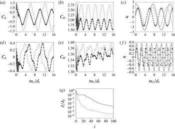
Figure 11. Results for DA experiments of type 3: temporal evolution of the lift coefficient (a,d), drag coefficient (b,e) and dimensionless rotational speed $\unicode[STIX]{x1D6FC}$ of the cylinder (c,f) for reference (○), first-guess (– – – –) and assimilated (——) runs; (g) cost function $J$ in (2.15) versus the iteration of the optimization process for runs 3A (——) and 3B (– – – –). (a–c) Refer to run 3A (lock-on), while (d–f) refer to run 3B (non-lock-on).

DA experiments of type 3 investigate the possibility of reconstructing flows past a rotationally oscillating cylinder from the observation of integrated quantities such as the aerodynamic coefficients $C_{L}$ and $C_{D}$ . As in § 4.1.1, the control vector in the DA procedures is formed by the initial flow field and the three parameters in (3.1). The temporal Fourier transform of the lift coefficient $C_{L}$ is reported in figure 5(e,b) for the lock-on and non-lock-on regimes, respectively. Similarly as for the wake flow, in the lock-on regime, the temporal evolution of the lift coefficient is entirely determined by the oscillations of the cylinder, while for the non-lock-on case the dominant frequency is almost identical to the natural one, even if the frequency of the oscillations of the cylinder seems to have more importance here than in the vortex shedding (see figure 5 a). If we now consider the results of the DA procedures in figure 11, it appears that, except at the very beginning of the assimilation window, the assimilated temporal evolution of the coefficients $C_{L}$ and $C_{D}$ almost perfectly matches the reference ones for both runs 3A and 3B. The spurious oscillations at the beginning of the assimilation window are due to the finite frequency of observation (Mons et al. Reference Mons, Chassaing, Gomez and Sagaut2016), and we can notice that the assimilated solution always passes through the reference values at observation times. However, for both runs, even in the case where both the reference and first-guess runs are in the lock-on region (run 3A), the optimization procedure fails to recover the rotational speed of the reference flow. Similarly to the results of § 4.1.3, the optimization procedure has modified the initial condition of the first-guess flow in order to match the observations of the reference flow, which compensates for the lack of reconstruction of the reference rotational speed. The good fit to the observations is confirmed in figure 11(g), and it appears from the comparison between figures 4(e) and 11(g) that, for the present case, the low dimension of the observations allows us to obtain a greater error reduction than in the experiments of type 1 with the same computational cost. The present results suggest that there is no unicity of the solution of the DA problem in the case where both the initial condition (encompassing upstream conditions) and the rotational speed of the cylinder (even parameterized) of the reference flow are unknown and the aerodynamic coefficients are observed. This may be due to the very low dimension of the observations compared to that of the control vector in this case.

5.1 Control on the rotational speed at all times

5.1.1 Experiments with four sensors (type 4)

Figure 12. Results for experiment 4A ( ${\mathcal{A}}=2$ and ${\mathcal{F}}=0.165$ for the first-guess flow, lock-on). Results of the observation optimization procedure: (a) initial (white dots) and optimized (black dots) positions of velocity sensors in the vorticity field of the first-guess flow at $tu_{r}/d_{r}=10$ ; (b) cost function $G$ in (2.11) versus the iteration of the optimization process. Results of DA procedures: (c) dimensionless rotational speed $\unicode[STIX]{x1D6FC}$ of the cylinder for reference (○), first-guess ( $\cdots \cdots$ ) and assimilated runs obtained with the initial (– – – –) and optimized (——) configurations of velocity sensors; (d) cost function $J$ in (2.15) versus the iteration of the optimization process with the initial (– – – –) and optimized (——) configurations of velocity sensors.

We first examine the results of the numerical experiments of type 4 where the control vector in the DA procedure is formed by the rotational speed of the cylinder at all times, and the initial condition of the reference flow is assumed to be known. Accordingly, the observation optimization procedure is used to increase the sensitivity of the observations, here four velocity sensors, with respect to changes in the rotational speed of the cylinder. Results for the configuration A ( ${\mathcal{A}}=2$ and ${\mathcal{F}}=0.165$ for the first-guess flow) of table 5 (run 4A) are reported in figure 12. The first step of this experiment, i.e. the observation optimization procedure, is illustrated in figure 12(a,b). The initial configuration of sensors, which is reported in white dots in figure 12(a), is chosen symmetric and close to the centreline of the wake. Figure 12(b) illustrates the evolution of the cost function $G$ defined in (2.11) during the corresponding optimization process, and its value is increased by a factor of almost five in three iterations. The corresponding optimized configuration of sensors is reported in black dots in figure 12(a). The sensors which were the closest to the cylinder have been placed further upstream by the optimization procedure, which allows us to increase the sensitivity of the sensors with respect to the rotational speed of the cylinder at the end of the assimilation window, as discussed below. On the whole, it seems that the four sensors have been brought closer to the shedded vortices. It is noticeable that the optimized configuration of sensors is asymmetric, contrary to the initial one. This may be explained by the finite size of the assimilation window, and it is expected that the optimized configuration tends to be symmetric for longer assimilation windows. This statement is confirmed in § 5.1.2.

Table 7. Number of iterations of the DA procedure $N_{DA}$ , reduction in the value of the cost function in (2.15)  $J/J_{0}$ , and reduction in the error on the reference rotational speed $\unicode[STIX]{x1D716}^{\unicode[STIX]{x1D714}_{c}}/\unicode[STIX]{x1D716}_{0}^{\unicode[STIX]{x1D714}_{c}}$ , as defined in (3.4), achieved by DA experiments performed with the first-guess configuration of sensors and with the configuration obtained by the observation optimization procedure in experiments of type 4–6. For the DA experiments using the optimized configurations of sensors, the number of iterations of the observation optimization procedure $N_{OO}$ and the increase in the cost function in (2.11)  $G/G_{0}$ are also reported, along with the total number of calls to the adjoint code $N_{tot}=N_{DA}+N_{OO}$ .

We now consider the second step of this experiment. Two different DA experiments are performed, using either the first-guess or optimized measurement network, in order to assess the efficiency of the observation optimization procedure, the results of which are illustrated in figure 12(c,d). The DA experiment using the optimized configuration of sensors achieves a better reconstruction of the reference solution than the one using the first-guess observation network, which is confirmed in table 7, where is reported the reduction in the error on the reference rotational speed achieved by the two DA procedures. However, in both cases, the optimization process does not recover the reference temporal evolution of the oscillations of the cylinder at the end of the assimilation window. This is due to the distance between the cylinder and the sensor networks, similarly as in § 4.1.3. For the first-guess configuration of sensors, the closest sensors to the cylinder are located at a distance of $2d_{r}$ from the latter. Accordingly, as in § 4.1.3, if we assume that the characteristic speed of transport of information from the cylinder to the observations is given by $u_{r}$ , the observations should be insensitive to changes in the rotational speed of the cylinder after $t=14d_{r}/u_{r}$ , and the DA procedure should not modify the first-guess solution after this time, which is confirmed by figure 12(c). Concerning the optimized sensor network, the closest sensor to the cylinder is located at a distance of $\simeq 1d_{r}$ , which implies that in this case the optimization process should not alter the first-guess rotational speed after $t=15d_{r}/u_{r}$ . The fact that sensors are placed further upstream in the optimized configuration therefore allows us a better reconstruction of the reference flow at the end of the assimilation window, as illustrated in figure 12(c). Furthermore, for the same final error reduction in the cost function $J$ in (2.15) ( $J/J_{0}=10^{-2}$ ), the DA procedure using the optimized configuration converges in fewer iterations than the one using the first-guess configuration. As indicated in table 7, even when taking into account the computational cost of the observation optimization procedure, the complete process of observation optimization followed by a DA procedure requires fewer calls to the adjoint code than directly performing a DA experiment with the initial configuration of sensors. Accordingly, the observation optimization procedure is efficient in terms of both computational cost and reconstruction of the reference flow in this case.

Figure 13. Results for experiment 4C ( ${\mathcal{A}}=2$ and ${\mathcal{F}}=0.375$ for the first-guess flow, lock-on). Results of the observation optimization procedure: (a) initial (white dots) and optimized (black dots) positions of velocity sensors in the vorticity field of the first-guess flow at $tu_{r}/d_{r}=10$ ; (b) cost function $G$ in (2.11) versus the iteration of the optimization process. Results of DA procedures: (c) dimensionless rotational speed $\unicode[STIX]{x1D6FC}$ of the cylinder for reference (○), first-guess ( $\cdots \cdots$ ) and assimilated runs obtained with the initial (– – – –) and optimized (——) configurations of velocity sensors; (d) cost function $J$ in (2.15) versus the iteration of the optimization process with the initial (– – – –) and optimized (——) configurations of velocity sensors.

Now, the observation optimization procedure is further tested with experiment 4C, where reference and first-guess flows different from those in run 4A are used ( ${\mathcal{A}}=2$ and ${\mathcal{F}}=0.375$ for the first-guess flow). The observation optimization procedure whose results are illustrated in figure 13(a,b) is initialized with the same first-guess configuration of sensors as for run 4A. In this case, the observation optimization procedure has increased by two orders of magnitude the value of the cost function $G$ in (2.11) in three iterations of the optimization process (figure 13 b). The corresponding optimized configuration of sensors is reported in figure 13(a). It could be expected that such an increase in the value of $G$ implies significant differences between the results of the DA procedures performed with the initial and optimized configurations of sensors, which is confirmed in figure 13(c,d). The DA procedure using the first-guess configuration has great difficulties in retrieving the reference solution, and the time evolution of the assimilated rotational speed of the cylinder is very spiky. In fact, the error on the reference rotational speed has increased during the optimization procedure, and the value of the cost function $J$ in (2.15) has decreased by less than an order of magnitude in 300 iterations, as indicated in table 7. In contrast, the DA procedure performed with the optimized configuration of sensors achieves a reduction in the value of the cost function $J$ by three orders of magnitude in the same number of iterations. Moreover, even if the assimilated rotational speed still does not perfectly match the reference one, the reduction in the error $\unicode[STIX]{x1D716}^{\unicode[STIX]{x1D714}_{c}}$ in (3.4) is significant. As for run 4A, the lack of reconstruction at the end of the assimilation window is due to the distance between the cylinder and the sensors. In the present case, the observation optimization procedure is thus particularly useful, since the optimized configuration of sensors allows us to correctly solve the DA problem, whereas the DA experiment performed with the first-guess configuration failed to retrieve the reference flow realization.

5.1.2 Sensitivity to the data assimilation set-up

Figure 14. Results for complementary observation optimization procedures performed with a similar set-up to that of experiment 4A: procedures (a,b) with a different initial configuration of sensors or (c,d) where the size of the assimilation window has been doubled. (a,c) The initial (white dots) and optimized (black dots) positions of the velocity sensors are reported in the vorticity field of the first-guess flow at $tu_{r}/d_{r}=10$ ; (b,d) cost function $G$ in (2.11) versus the iteration of the optimization procedure.

Two complementary observation optimization procedures are performed to investigate the influence of the choice of the first-guess configuration of sensors and that of the size of the assimilation window on the optimized configuration. The set-up of these computations is similar to that of experiment 4A, and the corresponding results are reported in figure 14. For the case illustrated in figure 14(a,b), a different first-guess configuration of sensors is employed, and the sensors are initially placed outside of the wake of the cylinder. Similarly to figure 12(a), the observation optimization procedure tends to place the sensors closer to the shedded vortices. However, the optimized configurations in figures 12(a) and 14(a) are not identical, while all the parameters of the corresponding experiments are the same. This suggests that the cost function $G$ has multiple local maxima and that the solution of (2.11) is not unique. In figure 14(c,d), the initial configuration of sensors is the same as in figure 12(a), but the size of the assimilation window has been doubled, and the simulations are performed until $t=T=32d_{r}/u_{r}$ instead of $16d_{r}/u_{r}$ . As anticipated, the optimized configuration of sensors appears less asymmetric in this case than in figure 12(a). More generally, more symmetric optimized sensor configurations are expected when the size of the assimilation window is large compared to the characteristic period of the oscillations. This statement is confirmed in § 5.2.1.

5.2 Control on the initial condition and the parameterized rotational speed of the cylinder

5.2.1 Experiments with four sensors (type 5)

Figure 15. Results for experiment 5D ( ${\mathcal{A}}=1$ and ${\mathcal{F}}=0.1$ for the first-guess flow, lock-on). Results of the observation optimization procedure: (a) initial (white dots) and optimized (black dots) positions of velocity sensors in the vorticity field of the first-guess flow at $tu_{r}/d_{r}=10$ ; (b) cost function $G$ in (2.11) versus the iteration of the optimization process. Results of DA procedures: (c) dimensionless rotational speed $\unicode[STIX]{x1D6FC}$ of the cylinder for reference (○), first-guess ( $\cdots \cdots$ ) and assimilated runs obtained with the initial configuration of velocity sensors (– – – –) and optimized configuration with merged sensors (——); (d) cost function $J$ in (2.15) versus the iteration of the optimization process with the initial configuration of sensors (– – –), optimized configuration (– ⋅ – ⋅ –) and optimized configuration with merged sensors (——).

For the experiments of type 5–6 (see table 6) the control vector in the DA procedure is formed by the initial flow field and the three parameters characterizing the rotational speed of the cylinder according to (3.1). In these experiments, the optimization observation procedure of table 2 is thus used to increase the sensitivity of velocity sensors with respect to both the initial flow field and the rotational speed of the cylinder. The experiments of type 5 are first examined. Four velocity sensors are used to observe the flow, and various reference and first-guess solutions are considered. Results for configuration D ( ${\mathcal{A}}=1$ and ${\mathcal{F}}=0.1$ for the first-guess flow) of table 5 (run 5D) are illustrated in figure 15. The initial configuration of sensors for the observation optimization procedure (see figure 15 a,b) seems to be a relatively good first guess since the cost function $G$ has been increased by a factor of two by the optimization process, which is relatively low compared with the experiments of type 4. It is noticeable that the observation optimization procedure has clustered the sensors of the optimized configuration in a single location. In order to assess the previous results, three DA experiments are performed: the first experiment uses the first-guess configuration of sensors, the second experiment directly uses the optimized configuration with four sensors, and the third experiment employs the optimized configuration where the four sensors are merged into one single sensor. Even with a merged single sensor, the DA experiments performed with the optimized configuration achieve a better reconstruction of the reference rotational speed of the cylinder than the DA experiment using the first-guess configuration (see figure 15 c and table 7). Besides, the DA experiments performed with the optimized configuration reach the same error reduction $J/J_{0}$ in slightly fewer iterations than with the initial configuration.

Figure 16. Results for experiment 5A ( ${\mathcal{A}}=2$ and ${\mathcal{F}}=0.165$ for the first-guess flow, lock-on). Results of the observation optimization procedure: (a) initial (white dots) and optimized (black dots) positions of velocity sensors in the vorticity field of the first-guess flow at $tu_{r}/d_{r}=10$ ; (b) cost function $G$ in (2.11) versus the iteration of the optimization process. Results of DA procedures: (c) dimensionless rotational speed $\unicode[STIX]{x1D6FC}$ of the cylinder for reference (○), first-guess ( $\cdots \cdots$ ) and assimilated runs obtained with the initial configuration of velocity sensors (– – – –) and optimized configuration with merged sensors (——); (d) cost function $J$ in (2.15) versus the iteration of the optimization process with the initial configuration of sensors (– – – – ), optimized configuration (– ⋅ – ⋅ –) and optimized configuration with merged sensors (——).

Results for experiment 5A are illustrated in figure 16. This experiment uses the same first-guess flow and first-guess configuration of sensors as experiment 4A, and it is interesting to note the differences between the obtained optimized configurations of sensors when the observation optimization procedure is used to increase the sensitivity of the sensors with respect to only the rotational speed of the cylinder (see figure 12 a,b) or with respect to both the initial flow field and the rotational speed of the cylinder (see figure 16 a,b). Compared to the former case, the observation optimization procedure has placed the velocity sensors further upstream in the latter case. This may be explained by the fact that the region of the initial flow in front of the cylinder form the upstream conditions for the wake flow during the considered time interval, as detailed in § 3.3. In addition, it may be worth keeping in mind that the considered flow configuration is convection-dominated. Upstream conditions may significantly affect the vortex shedding, as illustrated in § 4.1.3 and figure 8, where it appears that the DA procedure may fit the available observations of the velocity field by only adjusting the initial field, in particular for the non-lock-on case. Accordingly, as bringing the sensors closer to the cylinder increases the sensitivity of the observations with respect to its rotational speed at the end of the assimilation window, see §§ 4.1.3 and 5.1, performing measurements further upstream may improve their sensitivity with respect to the characteristics of the incoming flow at latter times. Two pairs of close sensors can be identified above and below the cylinder in the optimized configuration, and, similarly to experiment 5D, the optimized configuration is used in the DA experiments either directly or with two merged sensors. As indicated in table 7 and illustrated in figure 16(c,d), the DA experiments using the optimized configuration of sensors achieve almost the same reduction in the error on the reference rotational speed as with the first-guess configuration, but three times fewer iterations of the optimization process are required in the former case. As for experiment 5D, merging the close sensors does not significantly degrade the optimality of the observation network.

Figure 17. Results for experiment 5C ( ${\mathcal{A}}=2$ and ${\mathcal{F}}=0.375$ for the first-guess flow, lock-on). Results of the observation optimization procedure: (a) initial (white dots) and optimized (black dots) positions of velocity sensors in the vorticity field of the first-guess flow at $tu_{r}/d_{r}=10$ ; (b) cost function $G$ in (2.11) versus the iteration of the optimization process. Results of DA procedures: (c) dimensionless rotational speed $\unicode[STIX]{x1D6FC}$ of the cylinder for reference (○), first-guess ( $\cdots \cdots$ ) and assimilated runs obtained with the initial (– – – –) and optimized (——) configurations of velocity sensors; (d) cost function $J$ in (2.15) versus the iteration of the optimization process with the initial (– – – –) and optimized (——) configurations of velocity sensors.

The use of the configuration C of table 5 (run 5C) is examined in figure 17. Similarly to experiment 4C where the same first-guess flow is considered, the observation optimization procedure has increased the value of the cost function $G$ by two orders of magnitude. The optimized configuration of sensors of figure 17(a) appears more symmetric than in figure 13(a). As illustrated in figure 17(d), the DA procedure performed with the optimized configuration of sensors converges at a much faster rate towards the reference flow than the one using the first-guess observation network. Indeed, 29 and 163 iterations of the optimization process are required in the former and latter cases, respectively, to achieve the error reduction $J/J_{0}=10^{-2}$ . Besides, the error reduction on the reference rotational speed at the end of the optimization procedure is five times greater in the case where the optimized sensors are used than in the case where the first-guess observation network is employed. As summarized in table 7, the use of the observation optimization procedure is largely cost efficient in terms of both total number of calls to the adjoint code and reconstruction of the reference flow in this case.

Figure 18. Results for experiment 5B ( ${\mathcal{A}}=0.5$ and ${\mathcal{F}}=0.5$ for the first-guess flow, non-lock-on). Results of the observation optimization procedure: (a) initial (white dots) and optimized (black dots) positions of velocity sensors in the vorticity field of the first-guess flow at $tu_{r}/d_{r}=10$ ; (b) cost function $G$ in (2.11) versus the iteration of the optimization process. Results of DA procedures: (c) dimensionless rotational speed $\unicode[STIX]{x1D6FC}$ of the cylinder for reference (○), first-guess ( $\cdots \cdots$ ) and assimilated runs obtained with the initial (– – – –) and optimized (——) configurations of velocity sensors (the two latter curves overlap each other); (d) cost function $J$ in (2.15) versus the iteration of the optimization process with the initial (– – – –) and optimized (——) configurations of velocity sensors.

While the previous experiments in the present section were dedicated to the reconstruction of flows in the lock-on regime, we now investigate the possibility of employing the proposed observation optimization procedure in the non-lock-on one. To this end, we consider the configuration B ( ${\mathcal{A}}=0.5$ and ${\mathcal{F}}=0.5$ for the first-guess flow) of table 5 (run 5B) and the results of figure 18. It appeared from the results of § 4.1.1 that in this case the reference rotational speed of the cylinder cannot be satisfactorily recovered from observations of the velocity field in the cylinder wake due to the fact that the oscillations of the cylinder do not directly determine the vortex shedding, the latter being dominated by a frequency almost identical to the natural one. However, figure 5(c) indicates that, close enough to the cylinder, the frequency of its oscillations is predominant in the temporal evolution of the flow, even if the latter remains multi-frequency. Accordingly, instead of placing velocity sensors in the cylinder wake as in the previous experiments, measurements are initially performed in the vicinity of the cylinder for run 5B, as illustrated in figure 18(a). The sensor network obtained by the observation optimization procedure is also reported in figure 18(a), and it appears that the optimization process has maintained the symmetry of the measurement network. A symmetric optimized configuration of sensors is expected in the case where $Tf\gg 1$ , where $T$ is the size of the assimilation window and $f$ the frequency of the oscillations of the cylinder in (3.1), which is coherent with the present results. The most asymmetric sensor configuration is obtained with run 5D (see figure 15 a), which is associated to the lowest investigated frequencies; more symmetric configurations are obtained in runs 5A and 5C (see figures 16 a and 17 a, respectively), while run 5B corresponds to both the highest investigated frequencies and the most symmetric optimized sensor network. As illustrated in figure 18(c), the DA experiments relying on either the initial or optimized sensor configurations have both satisfactorily reconstructed the reference rotational speed of the cylinder and have achieved a similar reduction in the error on the reference flow. These results confirm the possibility of correctly reconstructing flows in the non-lock-on regime when measurements are performed in a region where the oscillations of the cylinder have a more important influence on the flow compared to locations, such as in the cylinder wake, where the flow is fully desynchronized with the oscillations of the cylinder. Furthermore, figure 18(d) indicates that the use of the optimized sensor network allows us to speed up the convergence of the DA process, and two time fewer iterations of the optimization procedure are required to reach the same error reduction $J/J_{0}$ as with the initial configuration of sensors.

5.2.2 Experiments with 20 sensors, sensor selection (type 6)

Figure 19. Results for experiment 6A ( ${\mathcal{A}}=2$ and ${\mathcal{F}}=0.165$ for the first-guess flow, lock-on). Results of the observation optimization procedure: (a) initial configuration of velocity sensors (white dots), (b) optimized velocity sensors (black dots), and (c) optimized configuration with only the most important sensors; (d) cost function $G$ in (2.11) versus the iteration of the optimization process. Results of DA procedures: (e) dimensionless rotational speed $\unicode[STIX]{x1D6FC}$ of the cylinder for reference (○), first-guess ( $\cdots \cdots$ ) and assimilated runs obtained with the initial configuration of velocity sensors (– – –) and optimized configuration with only the most important sensors (——); (f) cost function $J$ in (2.15) versus the iteration of the optimization process with the initial configuration of sensors (– – – –), optimized configuration (– ⋅ – ⋅ –) and optimized configuration with only the most important sensors (——).

Figure 20. Results for experiment 6C ( ${\mathcal{A}}=2$ and ${\mathcal{F}}=0.375$ for the first-guess flow, lock-on). Results of the observation optimization procedure: (a) initial configuration of velocity sensors (white dots), (b) optimized velocity sensors (black dots), and (c) optimized configuration with only the most important sensors; (d) cost function $G$ in (2.11) versus the iteration of the optimization process. Results of DA procedures: (e) dimensionless rotational speed $\unicode[STIX]{x1D6FC}$ of the cylinder for reference (○), first-guess ( $\cdots \cdots$ ) and assimilated runs obtained with the initial configuration of velocity sensors (– – – –) and optimized configuration with only the most important sensors (——) (the two latter curves overlap each other); (f) cost function $J$ in (2.15) versus the iteration of the optimization process with the initial configuration of sensors (– – –), optimized configuration (– ⋅ – ⋅ –) and optimized configuration with only the most important sensors (——).

Finally, we consider experiments of type 6, whose set-up is similar to that of the experiments of type 5, but now 20 velocity sensors are used to perform the observations of the flow. Generally speaking, when increasing the number of sensors to observe a given system, one could expect discrepancies in the sensitivity with respect to changes in the system between the different sensors. In this respect, it may be interesting to quantify the importance of each sensor and to identify the most sensitive ones. The sensor selection procedure described in § 2.6 is here used to select the most important sensors in the optimized observation networks. Results for experiment 6A are reported in figure 19. Starting from the first-guess configuration of sensors illustrated in figure 19(a), the configuration of figure 19(b) is obtained with the observation optimization procedure. The increase in the value of the cost function $G$ achieved by the optimization procedure is moderate (by a factor 1.2) compared with the previous experiments using four sensors. Performing the observations with 20 sensors actually provides much more information about the flow than with four sensors, and it is expected that the gain in sensitivity obtained with observation optimization strategies becomes less drastic as the number of sensors increases. The most important sensors of the optimized configuration in the sense of (2.20)–(2.21) are selected with $\unicode[STIX]{x1D6FF}=0.997$ in figure 19(c). With this value, only 11 sensors remain, and we can notice that the removed sensors coincide with the ones of the first-guess configuration that have not been moved by the optimization process and were located the furthest from the shedded vortices. Three DA experiments are performed to assess the results of the observation optimization procedure, each using a sensor configuration among the three ones illustrated in figure 19(a–c). The corresponding results are reported in figure 19(e,f). The DA experiment performed with only the most important sensors of the optimized configuration achieves a better reconstruction of the reference rotational speed of the cylinder than the DA experiment using the first-guess configuration, and in fewer iterations, as summarized in table 7. Only retaining the most sensitive sensors does not appear to have significantly degraded the optimality of the observation network.

We finally consider the results of experiment 6C, which are illustrated in figure 20. The configuration of sensors obtained with the observation optimization procedure is illustrated in figure 20(b), starting from the same first-guess configuration as in experiment 6A. Quite surprisingly, some of the sensors have been placed relatively far from the cylinder and upstream or outside of the wake flow. When considering these results, it may be worth keeping in mind that the observation optimization procedure is used here to increase the sensitivity of the sensors with respect to both the rotational speed of the cylinder and the initial flow field. As discussed in § 5.2.1, as placing sensors closer to the cylinder may increase their sensitivity with respect to changes in the rotational speed of the cylinder, performing measurements further from the vortex shedding or upstream from the cylinder may enhance the sensitivity of the observations with respect to the initial condition and upstream conditions. Equations (2.20)–(2.21) with $\unicode[STIX]{x1D6FF}=0.95$ are considered to select the most important sensors in the optimized configuration. The value of $\unicode[STIX]{x1D6FF}$ is adjusted in order to remove nearly half of the sensors, as in run 6A. The resulting configuration is illustrated in figure 20(c), where 10 sensors remain. Results for DA procedures performed with the three configurations of sensors of figure 20(a–c) are reported in figure 20(e,f) and table 7. The DA experiments performed with the first-guess configuration and the optimized configurations of sensors have achieved a similar reduction in the error on the reference rotational speed of the cylinder, which is satisfactorily identified in both cases. However, the DA experiment with only the most important sensors of the optimized configuration has reached this error reduction in almost seven times fewer iterations than the DA experiment performed with the first-guess configuration. Even with two times fewer sensors than the first-guess configuration of sensors, the optimized configuration proves to be superior for DA purposes.