


1. Introduction
A long-standing challenge in falling film flows has been to develop simple and accurate models that capture their nonlinear wavy dynamics. There have been continued efforts by researchers to optimise the chemical engineering processes that involve these flows and obtain models that are based on the fundamental closure assumption for the streamwise velocity distribution – see the reviews by Kalliadasis et al. (Reference Kalliadasis, Ruyer-Quil, Scheid and Velarde2012), Noble & Vila (Reference Noble and Vila2013), Ruyer-Quil et al. (Reference Ruyer-Quil, Kofman, Chasseur and Mergui2014), Richard, Ruyer-Quil & Vila (Reference Richard, Ruyer-Quil and Vila2016) and Richard et al. (Reference Richard, Gisclon, Ruyer-Quil and Vila2019) for recent attempts. To the best of our knowledge, the four-equation model derived by Ruyer-Quil & Manneville (Reference Ruyer-Quil and Manneville2000) using a weighted residual method (WRM) is the most accurate. This model precisely captures the characteristics of the solitary waves that dominate and organise the noise-driven dynamics of falling films. Although the four-equation WRM model is fully consistent at second order, its complicated expression hampers its use in the film flow community. This inspired the development and wide use of a simplified two-equation WRM model, in spite of its moderate overestimation of the velocity of solitary waves. This two-equation model is hereinafter referred to as the Ruyer-Quil and Manneville (RQM) model.
In fact, two-equation models, which can be viewed as extensions to viscous flows of the Saint-Venant formalism of shallow-water flows, offer the most promising framework. This motivated Richard et al. (Reference Richard, Gisclon, Ruyer-Quil and Vila2019) to consider all consistent two-equation models that can be derived by in-depth integration of the momentum balance (momentum integral method or MIM) or by integration of the energy balance (energy integral method or EIM). They showed that it is possible to derive consistent two-equation models up to first order for inertia terms and second-order for viscous diffusion which present optimal mathematical properties (conservation equations preserving mathematical entropy). Although some formulations of two-equation models could accurately predict the asymptotic speed of solitary waves, none of them turned out to be fully satisfactory. In particular, reconstruction of the velocity field from this approach poses difficulty, as the derivation of these models is based on the asymptotics of the velocity. In principle, predictions of the flow field under the waves are thus limited to only small-amplitude waves and low values of the Reynolds number, where the long-wave expansion is strictly valid.
Conversely, Ruyer-Quil & Manneville (Reference Ruyer-Quil and Manneville2002) have shown that any WRM converges to a unique expression of the WRM models if the number of test functions is sufficient. In fact, the expressions of these models are entirely determined by the ansatz for the velocity profile across the film or closure hypothesis (Ruyer-Quil et al. Reference Ruyer-Quil, Kofman, Chasseur and Mergui2014). This raises the question of the quest for an educated guess for the velocity, yielding the best two-equation model within the WRM. This approach has the advantage to provide unambiguous information on the velocity field under the waves.
Recently, Usha, Chattopadhyay & Tiwari (Reference Usha, Chattopadhyay and Tiwari2020) have proposed an ellipse profile for the velocity field and derived a new first-order model by employing the EIM. The choice of ellipse profile as weight function in that study was motivated by the success of the EIM with an ellipse profile in accurately and effectively predicting the squeeze film force in squeeze flow problems and in predicting the inertial effects on the performance of squeeze film dampers (Han & Rogers Reference Han and Rogers1996). This choice allows for a free parameter in the velocity profile, which is related to the eccentricity of the ellipse, and this helps in adjusting the profile. The results reveal that, as this free parameter is increased but remains finite, there is significant improvement in the predictions in the inertia-dominant regimes.
In this paper, we introduce an adjustable velocity profile based on the elliptic profile and investigate how the eccentricity of this profile influences the properties of the resulting WRM models. A variant of the ellipse profile (see § 2) is employed for the velocity distribution, yielding a two-equation model with an adjustable parameter, which is referred to as the ellipse velocity profile (EVP) model. The EVP model, though consistent at first order for inertia and at second order for viscous terms, does not present the expected structure of a shallow-water model, where convective terms are quadratic with respect to the velocity (or flow rate  $q$) and diffusion terms are linear with respect to
  $q$. A modified model (EVPM) having this structure is proposed instead. As a first step in assessing the performance of the derived models, the characteristics of single-hump solitary wave solutions are obtained and are compared with the characteristics of the direct numerical simulation (DNS) of the Navier–Stokes equations presented by Chakraborty et al. (Reference Chakraborty, Nguyen, Ruyer-Quil and Bontozoglou2014).
2. Mathematical modelling
We consider a liquid film flowing down a plane making an angle  $\beta$ with the horizontal. The fluid properties, i.e. kinematic viscosity
  $\nu =\mu /\rho$, density
  $\rho$ and surface tension
  $\sigma$, are constant. At the free surface, the gas is considered to be passive, with a constant pressure. We assume a slow evolution of the liquid film in space and time and introduce a film parameter
  $\varepsilon$ as a formal parameter, which is inserted along with each derivative
  $\partial _x$ and
  $\partial _t$ in space and time. This allows us to apply Prandtl's simplification of the cross-stream momentum balance, which gives
 \begin{gather} \varepsilon\delta (u_t + u u_x + v u_y) = b(h) + u_{yy} + \varepsilon^2 \eta (2u_{xx} + [ u_x|_{y=h} ]_x), \end{gather}
 \begin{gather}u_x + v_y = 0, \quad u|_{y=0}= v|_{y=0}, \end{gather}
 \begin{gather}u_y|_{y=h} = \varepsilon^2\eta (4 h_x u_x|_{y=h} - v_x|_{y=h}),\quad v|_{y=h} = h_t + u|_{y=h} h_x. \end{gather}
Here  $b(h) = 1 - \varepsilon \zeta h_x + \varepsilon ^3 h_{xxx}$ combines the streamwise gravity acceleration (body force) and a pressure gradient with a hydrostatic part and a contribution of surface tension.
System (2.1) is obtained after elimination of the pressure field and is consistent up to  $O(\varepsilon ^2)$ (Ruyer-Quil & Manneville Reference Ruyer-Quil and Manneville2000). We chose to write (2.1) using Shkadov's notation, for which the time
  $t$ and the streamwise coordinate
  $x$ have been compressed by a ratio
  $\kappa = (l_c/h_N)^{2/3}$, where
  $l_c=\sqrt {\sigma /(\rho g \sin (\beta ))}$ is a capillary length and
  $h_N$ is the thickness of the uniform film (Nusselt solution). The spatial coordinates
  $x$ and
  $y$ have been made dimensionless with the scales
  $\kappa h_N$ and
  $h_N$, respectively. The time scale is
  $\kappa h_N/u_N$, where
  $u_N=g \sin (\beta ) h_N^2/\nu$ is three times the averaged speed of the Nusselt solution, which corresponds to the speed of kinematic waves at the free surface in the very-long-wave limit. Similarly, the velocity components
  $u$ and
  $v$ have been made dimensionless with the scales
  $u_N$ and
  $u_N/\kappa$, respectively. This choice of scales enables us to limit significantly the number of coefficients in (2.1) differing from unity. In particular,
  $\kappa$ is adjusted so that the surface tension term bears a coefficient equal to one.
Three dimensionless groups characterise the flow: the reduced Reynolds number  $\delta = 3 Re/\kappa$, where
  $Re = u_N h_N/(3 \nu )$ is the Reynolds number based on the averaged velocity
  $u_N/3$; a reduced slope
  $\zeta = \cot (\beta )/\kappa$; and a parameter
  $\eta = 1/\kappa ^2$ that compares viscous diffusion and capillary damping of the waves. The reduced Reynolds number
  $\delta$ compares inertia and viscosity at a scale where surface tension is dominant. Ooshida (Reference Ooshida1999) showed that
  $\delta$ discriminates between two different regimes for which travelling waves present different tail lengths and properties, which he called the ‘drag–gravity’ and ‘drag–inertia’ regimes. Finally, we introduce the Kapitza number
  $Ka = \sigma /(\rho \nu ^{4/3} g^{1/3})$, which compares surface tension, viscosity and gravity. This parameter depends only on the fluid properties.
The Nusselt flat-film flow solution can be written as
 \begin{equation} u = h^2 \left(\frac{y}{h} - \frac{1}{2}\frac{y^2}{h^2} \right) \equiv h^2 g_0({\bar{y}}), \quad \text{where}\ \bar{y} =y/h. \end{equation}
The velocity is then parametrised with only one field, namely the film thickness  $h$, which is also the amplitude of the long-wave surface mode of instability. Yet, the velocity distribution of large-amplitude waves may significantly depart from the Nusselt solution. This is an effect of the inertia of the film. An easy way to account for this effect is to parametrise the velocity distribution with another field, usually the flow rate
  $q=\int _0^h u \,{{\rm d}y}$ or the averaged velocity
  $\bar {u} = q/h$.
Following Ruyer-Quil et al. (Reference Ruyer-Quil, Kofman, Chasseur and Mergui2014), we decompose the streamwise velocity into a main part and a correction,
 \begin{equation} u = u^{(0)}(h,q) + \varepsilon u^{(1)}(h,q) \equiv h^2 g_0({\bar{y}}) + \left(\frac{q}{h} - \frac{h^2}{3} \right) f_A(\bar{y}) + \varepsilon u^{(1)}(h,q), \end{equation}
where  $f_A$ refers to the ellipse-type velocity profile proposed by Usha et al. (Reference Usha, Chattopadhyay and Tiwari2020):
 \begin{align} f_A = K_p \left[\sqrt{A^2 - 4(\bar{y} -1)^2} - B \right], \quad\text{with}\ K_p = \frac{1}{\tfrac{1}{4}{A^2} \sin^{{-}1}({2}/{A}) - \tfrac{1}{2} B }, \quad B=\sqrt{A^2 - 4}. \end{align}
The ellipse velocity profile  $f_A$ and corrections
  $u^{(1)}$ fulfil the
  $O(\varepsilon )$ boundary conditions for the velocity and integral conditions:
 \begin{equation} \int_0^1 f_A(\bar{y})\, {\rm d}\bar{y} =1,\quad f_A(0)=0,\quad \frac{{\rm d}\, f_A}{{\rm d}{\bar y}}(1)=0, \quad \int_0^h u^{(1)}(h,q)\, {{\rm d}y}=0. \end{equation}
 Consequently, (2.3) verifies  $q=\int _0^h u\,{{\rm d} y}$ such that this decomposition is unique. Note that
  $u^{(0)}$ coincides with the Nusselt solution (2.2) for
  $q=h^3/3$, which corresponds to the in-depth integration of (2.2). The profile
  $f_A$ involves only one free parameter
  $A$, which can be varied in the range
  $]2, \infty [$. In the limit
  $A\to 2$,
  $f_A$ approaches a circular shape (see figure 1a). Note that, as
  $A$ increases, the eccentricity of the ellipse approaches values closer to
  $1$ (Usha et al. Reference Usha, Chattopadhyay and Tiwari2020), and
  $f_A$ tends to a parabola as
  $A\to \infty$. The profiles for higher values of
  $A\ (= 5, 10)$ are closer to each other and almost coalesce with the parabolic profile.


We retain the non-vanishing terms of highest order, namely first-order inertial terms and second-order viscous diffusion ones. Although second-order inertia terms can be retained, these terms may lead to non-physical behaviour, with the loss of solitary wave solutions, as  $\delta$ is raised (Ruyer-Quil et al. Reference Ruyer-Quil, Kofman, Chasseur and Mergui2014):
 \begin{gather} \varepsilon u^{(1)}_{yy} = \varepsilon\delta (u^{(0)}_t + u^{(0)}\,u^{(0)}_x + v^{(0)}\,u^{(0)}_y) - b(h) - u^{(0)}_{yy} \nonumber\\ \qquad\, - \,\varepsilon^2 \eta (2u^{(0)}_{xx} + [ u^{(0)}_x|_{y=h} ]_x ) + O(\varepsilon^2), \end{gather}
 \begin{gather}\varepsilon u^{(1)}|_{y=0} = 0, \quad \varepsilon u^{(1)}_y|_{y=h} = \varepsilon^2\eta (4 h_x u^{(0)}_x|_{y=h} - v^{(0)}_x|_{y=h} ) + O(\varepsilon^3). \end{gather}
The resulting momentum balance (2.6a) is next averaged with a parabolic weight  $w= g_0(\bar {y})$, the solution to
  $w_{yy} = \mathrm {const.}$, since then
 \begin{equation} \int_0^h g_0 u^{(1)}_{yy}\, {{\rm d} y} = \tfrac{1}{2} u^{(1)}_y|_{y=h} -\int_0^h u^{(1)}\,{{\rm d}y} = \varepsilon\eta(2h_x u^{(0)}_x|_{y=h} - \tfrac{1}{2} v^{(0)}_x|_{y=h}). \end{equation}
 As a result, the computation of the correction  $u^{(1)}$, the solution to (2.6), is unnecessary to achieve consistency at order
  $O(\varepsilon )$. Since
  $w$ is not proportional to
  $u^{(0)}$, the WRM differs here from the EIM – see Ruyer-Quil, Chakraborty & Dandapat (Reference Ruyer-Quil, Chakraborty and Dandapat2012) and Samanta, Goyeau & Ruyer-Quil (Reference Samanta, Goyeau and Ruyer-Quil2013) for other examples of the WRM approach where weight and test functions differ. The obtained averaged momentum balance thus reads
 \begin{gather} \delta q_t = \delta \left[\left(\frac{G}{S} \frac{q^2}{h^2} - \frac{G_1}{S} q h - \frac{G_2}{S} h^4\right)h_x - \left(\frac{F}{S} \frac{q}{h} + \frac{F_1}{S} h^2\right)q_x \right] + \frac{h}{3 S}\left[b(h)- \frac{3q}{h^3}\right] \nonumber\\ \quad + \,\eta \left[\left(\frac{J}{S} \frac{q}{h^2} - \frac{J_1}{S} h\right)h_x^2 - \frac{K}{S} \frac{q_x h_x}{h} - \left(\frac{L}{S} \frac{q}{h} + \frac{L_1}{S} h^2\right) h_{xx} + \frac{M}{S} q_{xx} \right], \end{gather}
where the ordering parameter  $\varepsilon$ has been dropped for simplicity. The coefficients
  $F$,
$F$,  $G$, etc. are functions of the parameter
  $A$, the expressions of which are given in Appendix A.
Compared to the RQM model derived by Ruyer-Quil & Manneville (Reference Ruyer-Quil and Manneville2000), (2.8) contains deviatory terms that are not present there, corresponding to the coefficients  $G_1$,
  $G_2$,
  $F_1$,
  $J_1$ and
  $L_1$. These terms arise due to the non-self-similar nature of
  $u_0(h,q)$ in the ansatz (2.3) as the parabolic profile
  $3g_0$ differs from the elliptic profile
  $f_A$. In the limit
  $A\to \infty$,
  $f_\infty =3g_0$ and these terms vanish. Owing to these deviatory terms, the averaged momentum balance (2.8) differs from the expected form of an averaged momentum balance, akin to a viscous shallow-water equation (Gerbeau & Perthame Reference Gerbeau and Perthame2001), where convective terms are quadratic with respect to the velocity, or equivalently the flow rate
  $q$, and viscous diffusion terms are linear with respect to
  $q$.
$q$.
However, (2.8) can easily be rewritten in a form where convective terms are quadratic and diffusive terms are linear with respect to  $q$ by playing with the zeroth-order equivalence
  $q = h^3/3 + O(\varepsilon )$ to rewrite the inertia and diffusion terms while retaining consistency at
  $O(\varepsilon )$ for the former and
  $O(\varepsilon ^2)$ for the latter. The result reads
 \begin{gather} \delta q_t = \delta \left[\left(\frac{G - 3 G_1 - 9 G_2}{S}\right)\frac{q^2}{h^2} h_x - \left(\frac{F + 3 F_1}{S}\right)\frac{q}{h} q_x \right] + \frac{h}{3 S}\left[b(h)- \frac{3q}{ h^3}\right]\nonumber\\ \qquad\, +\,\eta \left[\left(\frac{J - 3 J_1}{S}\right)\frac{q}{h^2} h_x^2 - \frac{K}{S} \frac{q_x h_x}{h} - \left(\frac{L + 3 L_1}{S} \right) \frac{q}{h} h_{xx} + \frac{M}{S} q_{xx}\right]. \end{gather}
 Completed by the (exact) mass balance  $h_t + q_x = 0$, (2.8) or (2.9) form two-equation low-dimensional models, referred to as EVP and EVPM models, respectively. These models are consistent up to
  $O(\varepsilon )$ for inertial terms and up to
  $O(\varepsilon ^2)$ for diffusive ones. As a consequence, the threshold of instability,
  $\delta _c = \tfrac {5}{2} \zeta$, is accurately captured by the two models. These two models lead to the same linear stability analysis of the Nusselt flat-film solution (same dispersion relation). Moreover, the locations of the marginal stability curves based on this dispersion relation (not shown) are nearly unaffected by the value of
  $A$ for a wide range of parameters. This shows that the linear stability of the Nusselt film based on the EVP, EVPM and RQM models are nearly equivalent. Since the RQM model has been shown to accurately capture the solutions to the Orr–Sommerfeld problem (Ruyer-Quil & Manneville Reference Ruyer-Quil and Manneville2002), we conclude that our new formulations reproduce satisfactorily the primary instability of the film for all values of
  $A>2$. The variations of the coefficients of the driving force (
 $b$), convective quadratic terms (
 $q^2 h_x/h$,
  $q q_x/h$) and linear diffusive terms (
 $q h_x^2/h^2$,
  $h_x q_x/h$,
  $q h_{xx}/h$,
  $q_{xx}$) with respect to
  $A$ are illustrated in table 1, which shows an excellent convergence to the RQM model as
  $A$ is raised.
Table 1. Coefficients of (2.8) (EVP) and (2.9) (EVPM) compared with the RQM model (equation (14) in Ruyer-Quil et al. Reference Ruyer-Quil, Kofman, Chasseur and Mergui2014).

3. Results and discussion
The results from the EVP and EVPM models are obtained for a film over a vertical wall ( $\beta = 90^\circ$) for typical values of the Kapitza number (water–glycerol solution,
  $Ka = 193$; plain water,
  $Ka= 3400$; and liquid nitrogen,
  $Ka = 10\,000$). We use the software Auto07p (Doedel et al. Reference Doedel, Champneys, Fairgrieve, Kuznetsov, Sandstede and Wang2007) to construct travelling-wave solutions, i.e. waves with a constant speed and shape, as solutions to a dynamical system in the three-dimensional phase space spanned by
  $h$,
$h$,  $h'$ and
  $h''$, where the primes refer to the derivatives with respect to the coordinate
  $\xi = x - c t$ in a frame moving at the phase speed
  $c$. Notice that integration of the mass balance gives
  $q= c h + q_0$, where
  $q_0$ is a constant, which explains that the dynamic system is a function of
  $h$ and its derivatives only. Solitary waves are computed in the limit of a large computational domain, through a homoclinic bifurcation. The procedure is detailed in Kalliadasis et al. (Reference Kalliadasis, Ruyer-Quil, Scheid and Velarde2012). The wave profile of a typical solitary wave, connecting the Nusselt film of thickness
  $h=1$ to itself, is illustrated in figure 1(b). The maximum amplitude (
 $h_{max}$) and phase speed (
 $c$) of the one-hump solitary wave are displayed in figure 2 as a function of the reduced Reynolds number (
 $\delta$) for different values of the parameter
  $A$. In the drag–gravity regime, at low values of
  $\delta$,
  $c -1$ and
  $h_{max} -1$ are
  $\propto \delta ^{3/2}$ (Ruyer-Quil & Kalliadasis Reference Ruyer-Quil and Kalliadasis2012). Instead, at large values of
  $\delta$, the phase speed
  $c$ reaches a plateau for which the amplitude
  $h_{max}$ continues to grow slowly, which corresponds to the drag–inertia regime.

Figure 2. Characteristics of solitary waves: (a,b) amplitude  $h_{max}$; (c,d) phase velocity
  $c$; (a,c) influence of varying
  $A$ for
  $\eta = 0.01$; and (b,d) comparison to DNS on varying
  $Ka$ for
  $A = A^\star =2.23219$; for all panels,
  $\theta = 90^\circ$. In panels (a,c) dashed lines are for (2.8) (EVP) and solid lines are for (2.9) (EVPM). In panels (b,d) solid lines are for (2.9) (EVPM), dotted lines are for RQM model, and dashed lines are for DNS (Chakraborty et al. Reference Chakraborty, Nguyen, Ruyer-Quil and Bontozoglou2014).
Figure 2(a,c) shows how the adjustable parameter  $A$ affects the speed and amplitude of the waves. For
  $\delta \lessapprox 1$, all curves fall on a master curve. This is expected, since, in the drag–gravity regime, inertia is weak, viscosity is high and the wave dynamics is slaved to its kinematics so that the long-wave expansion holds accurately. Therefore, all models consistent with the long-wave expansion give very close results in that regime. However, for
  $\delta \gtrapprox 1$, inertia is dominant and the influence of
  $A$ is significant. The asymptotic speed
  $\lim _{\delta \to \infty } c \equiv c_\infty$ increases with
  $A$ and reaches a maximum as the EVP and EVPM models converge to the RQM model (
 $c_\infty \approx 2.738$). The EVPM model systematically predicts larger wave amplitudes than the EVP model.
Ruyer-Quil & Manneville (Reference Ruyer-Quil and Manneville2005) have shown that the asymptotic speed  $c_\infty$ is obtained when the second fixed point location
  $h_{II} = -1/2 + \sqrt {3(c-1/4)}$, at which gravity and viscous drag compensate each other (i.e.
  $q=h^3/3$), corresponds to the critical level at which inertia terms cancel out, which gives
 \begin{equation} c^2 +\left(\frac{G - 3 G_1 - 9 G_2}{S}\right)\frac{h_{II}^4}{9} - c \left(\frac{F + 3 F_1}{S}\right)\frac{h_{II}^2}{3} = 0 \end{equation}
for both (2.8) and (2.9). Adjusting  $c_\infty$ to its prediction
  $2.560$ found by DNS gives
  $A = A^\star \approx 2.23219$. The DNS results obtained by Chakraborty et al. (Reference Chakraborty, Nguyen, Ruyer-Quil and Bontozoglou2014), along with the solutions to RQM model and to EVPM for
  $A = A^\star$, are presented for different Kapitza numbers in figure 2(b,d). Results from the EVP model, which somewhat underestimate the amplitude of solitary waves, are not shown. The choice of
  $A = A^\star$ for comparison is dictated by the requirement that the asymptotic speed
  $c_\infty$ of the models matches the predictions of DNS. Note that the dependence of the amplitude of the DNS results on the Kapitza number is an effect of the complex velocity distribution (departure from parabolic profile) under the capillary ripples. With two-equation models, such as EVP or EVPM models, there is no dependence of wave amplitude on the Kapitza number (no effect of capillarity on amplitude) and a monotonic behaviour of speed and amplitude with respect to the reduced Reynolds number
  $\delta$ is observed.
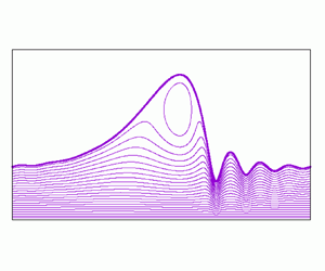
The performance of the EVPM model is further assessed by comparing its predictions to DNS for a large-amplitude travelling wave corresponding to an experiment performed by Dietze et al. (Reference Dietze, Al-Sibai and Kneer2009) in the drag–inertia regime ( $\delta =14.21$,
  $Ka = 509.5$). The DNS travelling-wave solution has been obtained by a projection method on Chebyshev polynomials and continuation method (see Cellier & Ruyer-Quil (Reference Cellier and Ruyer-Quil2020) for details). Figure 3(a) displays the wave profiles and streamlines in the moving frame computed from the modified model. The streamfunctions have been computed from the zeroth-order velocity distribution
  $u^{(0)}(h,q)$, as adding the correction
  $u^{(1)}$ reduces the agreement with DNS whenever the long-wave expansion does not strictly hold, as is the case for large-amplitude solitary waves (Ruyer-Quil et al. Reference Ruyer-Quil, Kofman, Chasseur and Mergui2014).

Figure 3. Streamlines in the laboratory and moving frames of a travelling-wave solution to (2.9) (EVPM) with  $A=A^\star$ corresponding to an experiment by Dietze, Al-Sibai & Kneer (Reference Dietze, Al-Sibai and Kneer2009): vertical wall, water–dimethyl sulfoxide (DMSO) mixture,
  $Re=15$,
  $f=16$ Hz,
  $\mu =3.13\times 10^{-3}$ Pa s,
  $\rho =1098.3~{\rm kg}~{\rm m}^{-3}$ and
  $\sigma =0.0484~{\rm N}~{\rm m}^{-1}$ (
 $\delta =14.21$,
  $\zeta =0$,
  $\eta =0.0876$ and
  $Ka = 509.5$). (a) Equation (2.9) (EVPM), moving frame; (b) DNS, moving frame; (c) equation (2.9) (EVPM), laboratory frame; and (d) DNS, laboratory frame.
The comparison with the DNS results is quite satisfactory, as evidenced by the predictions regarding the intensity and location of the recirculation zone in the main hump. The accumulation of capillary ripples at the foot of the solitary wave is well captured by the modified model (cf. figure 3c) and is in striking agreement with the corresponding DNS results (figure 3d). Streamlines in the laboratory frame (figure 3c,d) reveal the onset of back-flows, or separation eddies, at the locations of troughs in the capillary ripples preceding the main hump. Once again, the EVPM model captures remarkably well the flow pattern predicted by DNS, which shows that the EVP velocity profile  $u^{(0)}$ given by (2.3) is a satisfactory approximation of the true velocity profile.
4. Concluding remarks
Based on a combination of a parabolic and an ellipse profile introduced by Usha et al. (Reference Usha, Chattopadhyay and Tiwari2020), we have derived a new low-dimensional two-equation model for thin-film flows using the WRM. The model is first-order consistent for inertia terms and second-order consistent for diffusive terms, which guarantees that it captures the primary instability adequately. Equation (2.9) presents the usual structure for a shallow-water momentum balance, where convective terms are quadratic with respect to the flow rate  $q$ and diffusive terms are linear in
  $q$. The EVPM (2.9) successfully and satisfactorily captures the nonlinear wave properties of film flows down a vertical wall, in both the drag–gravity and drag–inertia regimes, such as asymptotic wave speed, maximum wave height, wave profiles, streamlines in the moving frame and the flow patterns in the laboratory frame. In particular, it is able to capture the onset of closed separation vortices which can form underneath the troughs of precursory capillary ripples (Dietze et al. Reference Dietze, Al-Sibai and Kneer2009).
This study is another step forward in the modelling of falling thin-film flows, thereby offering new perspectives for theoretical and applied investigations. This calls for further in-depth investigation of the EVPM model and similar formulations, taking full advantage of the adjustable ansatz for the velocity profile.
Acknowledgements
The authors thank S. Chakraborty, P.-K. Nguyen and V. Bontozoglou for providing them with the DNS results shown in figure 2.
Funding
C.R.-Q. acknowledges support from FRAISE project ANR-16-CE06-0011 of the French National Research Agency. S.M. thanks the Vellore Institute of Technology, Vellore, for providing the VIT SSEED Grant - RGEMS Fund (SG20220087) for carrying out this research work.
Declaration of interests
The authors report no conflict of interest.
Appendix A. Coefficients of EVP (2.8) and EVPM (2.9) models
 \begin{gather} S = \frac{16 B + 48 N -
3 A^2 N}{96 N},
\end{gather}
\begin{gather} S = \frac{16 B + 48 N -
3 A^2 N}{96 N},
\end{gather}
 \begin{gather}F = \frac{-16 (816 - 760
A^2 + 75 A^4) B + 30 A^2 (736 - 252 A^2 + 17 A^4) C + 45
A^6 B C^2}{720 B N^2},\\ F_1 =
\frac{1}{138240 N^2}[43008 + 405 A^8 C^2 + 128 A^2 ({-}3317
+ 816 B C)\nonumber\\ \quad\qquad\qquad\qquad -\, 180 A^6 ({-}9 + 9 B C + 76 C^2) +
240 A^4 (131 + 35 B C + 312 C^2)], \\ G = \frac{({-}576 + 520
A^2 - 30 A^4) B + 15 A^2 (64 - 20 A^2 + A^4) C}{60 B
N^2}, \end{gather}
\begin{gather}F = \frac{-16 (816 - 760
A^2 + 75 A^4) B + 30 A^2 (736 - 252 A^2 + 17 A^4) C + 45
A^6 B C^2}{720 B N^2},\\ F_1 =
\frac{1}{138240 N^2}[43008 + 405 A^8 C^2 + 128 A^2 ({-}3317
+ 816 B C)\nonumber\\ \quad\qquad\qquad\qquad -\, 180 A^6 ({-}9 + 9 B C + 76 C^2) +
240 A^4 (131 + 35 B C + 312 C^2)], \\ G = \frac{({-}576 + 520
A^2 - 30 A^4) B + 15 A^2 (64 - 20 A^2 + A^4) C}{60 B
N^2}, \end{gather}
 \begin{align}G_1 &= \frac{1}{11520 N^2}[9216 +
896 A^2 ({-}82 + 21 B C) + 15 A^4 (496\nonumber\\ &\quad + 36 A^2
+ 4 (4 - 9 A^2) B C +3 ({-}8 + A^2) ({-}32 + 3 A^2)
C^2)],\\ G_2 &={-}\frac{1}{46080 N^2} [6144 + 315
A^8 C^2 + 128 A^2 ({-}779 + 176 B C)\nonumber\\ &\quad - 60 A^6
({-}21 + 21 B C + 92 C^2) + 48 A^4 (65 + 145 B C + 488
C^2)],\\ J &= \frac{1}{24 B N^3}[{-}8 (56 + 13 A^2)
B^4 - 3 A^6 (16 + A^2) B C^3 + 128 A B^3 R\nonumber\\ &\quad + 4
A^2 B^2 C ((64 + 23 A^2) B - 32 A R) + 2 A^4 C^2 ({-}160 +
68 A^2 - 7 A^4 + 16 A B R)],\\ J_1 &={-}\frac{1}{36
B N^3}[4 A^2 B^2 (16 B + A ({-}64 + 64 A^2 - 19 A B)) C +
15 A^8 B C^3\nonumber\\ &\quad + 8 B^2 (32 - 76 A^2 + 17 A^4 - 32
A B V) -2 A^4 C^2 ({-}32 - 44 A^2 + 13 A^4 + 32 A B
V)],\\ K &= \frac{1}{12 (16 - 4 A^2 + A^4 C^2)}
[512 + 4 A (40 B + A ({-}52 + 5 A^2 - 8 A B))\nonumber\\ &\quad +
A^2 C ({-}64 B + 16 A (5 + A ({-}A + B)) + 3 A^4
C)],\\ L &= \frac{1}{24 N^3} [4 A^2 B (160 B + A
({-}176 + 16 A^2 - 7 A B)) C\nonumber\\ &\quad - 2 A^4 (80 B + A
({-}88 + A (8 A + B))) C^2 + 3 A^8 C^3 + 8 B^2 (5 B Q - 8 A
T)],\\ L_1 &= \frac{1}{144 N^3}[{-}640 A B^2 + 160
A^2 B^2 C + 32 A^7 C^2 - 15 A^8 C^3 + 128 A^3 B (B + 5
C)\nonumber\\ &\quad - 32 A^5 C (4 B + 5 C) + 2 A^6 C^2 (29 B + 36
C) - 4 A^4 B C (13 B + 64 C) - 8 B^3 Q], \end{align}
\begin{align}G_1 &= \frac{1}{11520 N^2}[9216 +
896 A^2 ({-}82 + 21 B C) + 15 A^4 (496\nonumber\\ &\quad + 36 A^2
+ 4 (4 - 9 A^2) B C +3 ({-}8 + A^2) ({-}32 + 3 A^2)
C^2)],\\ G_2 &={-}\frac{1}{46080 N^2} [6144 + 315
A^8 C^2 + 128 A^2 ({-}779 + 176 B C)\nonumber\\ &\quad - 60 A^6
({-}21 + 21 B C + 92 C^2) + 48 A^4 (65 + 145 B C + 488
C^2)],\\ J &= \frac{1}{24 B N^3}[{-}8 (56 + 13 A^2)
B^4 - 3 A^6 (16 + A^2) B C^3 + 128 A B^3 R\nonumber\\ &\quad + 4
A^2 B^2 C ((64 + 23 A^2) B - 32 A R) + 2 A^4 C^2 ({-}160 +
68 A^2 - 7 A^4 + 16 A B R)],\\ J_1 &={-}\frac{1}{36
B N^3}[4 A^2 B^2 (16 B + A ({-}64 + 64 A^2 - 19 A B)) C +
15 A^8 B C^3\nonumber\\ &\quad + 8 B^2 (32 - 76 A^2 + 17 A^4 - 32
A B V) -2 A^4 C^2 ({-}32 - 44 A^2 + 13 A^4 + 32 A B
V)],\\ K &= \frac{1}{12 (16 - 4 A^2 + A^4 C^2)}
[512 + 4 A (40 B + A ({-}52 + 5 A^2 - 8 A B))\nonumber\\ &\quad +
A^2 C ({-}64 B + 16 A (5 + A ({-}A + B)) + 3 A^4
C)],\\ L &= \frac{1}{24 N^3} [4 A^2 B (160 B + A
({-}176 + 16 A^2 - 7 A B)) C\nonumber\\ &\quad - 2 A^4 (80 B + A
({-}88 + A (8 A + B))) C^2 + 3 A^8 C^3 + 8 B^2 (5 B Q - 8 A
T)],\\ L_1 &= \frac{1}{144 N^3}[{-}640 A B^2 + 160
A^2 B^2 C + 32 A^7 C^2 - 15 A^8 C^3 + 128 A^3 B (B + 5
C)\nonumber\\ &\quad - 32 A^5 C (4 B + 5 C) + 2 A^6 C^2 (29 B + 36
C) - 4 A^4 B C (13 B + 64 C) - 8 B^3 Q], \end{align}
 \begin{gather}M = \frac{-48 B + 72 N +
A (64 - 3 A N)}{48 N},
\end{gather}
\begin{gather}M = \frac{-48 B + 72 N +
A (64 - 3 A N)}{48 N},
\end{gather}
where  $B = \sqrt {A^2 - 4}$,
  $C = \arctan ({2}/{B})$,
  $N = (A^2C - 2B)$,
  $R = A^2 + 5$,
  $V = A^2 -1$,
  $T = A^2 - 11$ and
  $Q = A^2 - 16$.


