


1. INTRODUCTION
This paper provides for the first time a closed-form solution of the health capital model of health demand. The model is also known as the Grossman model, named after the seminal paper of Grossman (Reference Grossman1972), which developed its main ingredients. In its long history the Grossman model has been criticized for various shortcomings and counterfactual predictions. Several of these (alleged) shortcomings have been addressed by further developments of the original model. The core mechanics of the Grossman model remained, until recently, basically unchallenged by the development of an alternative theory. Empirically, the Grossman model is the inspiration if not the foundation of many reduced-form and structural models of health demand.
The core mechanics of the Grossman model arise from the assumption that individuals accumulate health capital H in a similar fashion as they accumulate human capital in form of education. In any period or, in continuous time, in any instant of time, health capital depreciates and is potentially augmented by health investment. The health capital stock of an individual of age t thus evolves, in continuous time, according to
 $\dot{H}(t)= f(I(t))-\delta (t) H(t)$
, in which I is investment, f is a positive function, and δ is the depreciation rate. The key assumption is that the loss of health capital through depreciation is an increasing function of its stock. This means that of two individuals of the same age t, the one in better health, i.e. the one with the greater health stock H(t) loses more health capital in the next instant, since health depreciation δ(t)H(t) is increasing in H(t). Notice that this basic assumption is imposed independently from whether δ is considered to be constant or age-dependent.Footnote
1
$\dot{H}(t)= f(I(t))-\delta (t) H(t)$
, in which I is investment, f is a positive function, and δ is the depreciation rate. The key assumption is that the loss of health capital through depreciation is an increasing function of its stock. This means that of two individuals of the same age t, the one in better health, i.e. the one with the greater health stock H(t) loses more health capital in the next instant, since health depreciation δ(t)H(t) is increasing in H(t). Notice that this basic assumption is imposed independently from whether δ is considered to be constant or age-dependent.Footnote
1
Evidence from gerontology supports the reverse of the Grossman assumption. The accumulation of health deficits is found to be a positive function of the health deficits that are already present in an individual. Of two individuals of the same age the unhealthier one is predicted to lose more health (accumulate more health deficits) in the next instant. This law of health deficit accumulation has a micro-foundation in reliability theory and it is a very strong predictor of mortality (Mitnitski et al., Reference Mitnitski, Mogilner, MacKnight and Rockwood2002a, Reference Mitnitski, Mogilner, MacKnight and Rockwood2002b, Reference Mitnitski, Song, Skoog, Broe, Cox, Grunfeld and Rockwood2005, Reference Mitnitski, Bao and Rockwood2006).
Advocates of the health-capital model, however, could defend the approach based on Friedman’s (Reference Friedman1953) methodology of economic modeling, stating that a theory’s assumptions should not matter as long as its predictive quality is good. Generating testable predictions from the Grossman model, however, is a tough task. In order to appreciate this fact, notice that even the simplest version of the Grossman model generates two differential equations (or in discrete time two difference equations): one equation of motion for the health capital stock and one equation of motion generated from the first-order conditions for optimal health investment. The latter could be expressed as equation of motion for the shadow price of health, or health investment, or consumption. The solution is thus expressed as a trajectory in a two-dimensional phase space. The problem is that there are infinitely many trajectories fulfilling the first-order conditions, usually pointing in all possible directions in the phase space. In other words, based solely on the first-order conditions and the equation of motion for the state variable (i.e. health capital), the solution is indeterminate. The unique optimal solution of the Grossman model is identified by the transversality condition. This unique optimal solution allows to derive testable predictions of the model.
It is perhaps fair to say that most of the problems that the literature had with solving the Grossman model originated from an inappropriate use of the first-order conditions. Grossman (Reference Grossman1972) and some followers (e.g. Jacobson, 2000) just ignored the transversality condition, others had problems of applying it appropriately because they stated the health demand problem in discrete time (Ried, Reference Ried1998). Many empirical applications derived reduced-form or structural equations for health care demand from solving simplified versions of the first-order conditions and the equation of motion (Muurinen, Reference Muurinen1982; Wagstaff, Reference Wagstaff1986; Grossman, Reference Grossman, Culyer and Newhouse2000). But since there are infinitely many trajectories fulfilling the first-order conditions, any structural form obtained by ignoring the transversality condition is a result from (unwarranted) simplifications.Footnote 2
Some other studies suggested to reformulate the original Grossman model in order to reduce the difficulties involved with identification. The original Grossman model assumes that death is a free terminal condition. Death occurs when a minimum state of health is reached and health investment and the state of health influence the decline of health and thus the age at death T. For this problem, identification requires to solve the associated Hamiltonian function at the yet to be determined time of death. This difficult task is circumvented by assuming alternatively that individuals face a predetermined time of death, which occurs irrespective of their health, and then optimally chose the state of health H(T) that they want to experience when they die (e.g. Eisenring, Reference Eisenring1999; Kuhn et al., Reference Kuhn, Wrzaczek, Prskawetz and Feichtinger2012; van Kippersluis and Galama, Reference van Kippersluis and Galama2014). Clearly, an approach based on a predetermined time of death cannot lead to an informative reasoning about human aging and longevity. A rigorous analysis and critique of the effects of the different treatments of the transversality condition is provided by Forster (Reference Forster2001). Yet, even studies investigating the original Grossman model and stating one potentially appropriate transversality condition tend to ignore the full solution space because they assume at the outset that life ends at a finite T (Ehrlich and Chuma, Reference Ehrlich and Chuma1990; Forster, Reference Forster2001). As will be discussed below, the Grossman model usually allows for eternal life. This requires a different transversality condition to hold, which is usually fulfilled by the Grossman model.Footnote 3
So far, comparative statics of the Grossman model have been derived by phase diagram analysis or numerical methods. Clearly it is not possible to use these methods in order to derive (structural) equations for an estimation of the model. This paper proposes a different approach. It obtains a closed-form solution by imposing certain (iso-elastic) functional forms and a particular parametrization of the model. This provides non-simplified structural equations for empirical testing and allows to prove analytically not only the comparative statics but also the comparative dynamics of the model. Because the closed-form solution allows for an explicit verification of the transversality condition, it provides a theoretical identification of the optimal health-for-age trajectory and its determinants.
The closed-form solution is obtained for a particular value of the curvature parameter of the utility function σ, where 1/σ is known as the elasticity of intertemporal substitution. Given a plausible parametrization of the model, σ is between 1.5 and 2.5, depending on how much health matters for utility and for productivity. A value of σ in this range is supported by many empirical studies. A recent meta-analysis of 2,735 published estimates of the intertemporal elasticity of substitution found the world average of σ at 2.0 (Havranek et al., Reference Havranek, Horvath, Irsova and Rusnak2013).
Nevertheless, the question may arise how general the obtained results are. In order to address this problem, I show in the associated discussion paper (Strulik, Reference Strulik2014) that the steady state for health capital is generally independent of σ. This means that for any value of σ individual health behavior becomes more and more similar to the closed form solution as individuals age and their health approaches the steady state. The closed-form value of σ provides a threshold value that identifies whether health care investment increases or declines as individuals age and their health capital deteriorates. Health care expenditure increases if and only if the “true” σ lies below the threshold value. Moreover, extensive discussion of the general features of the health capital model confirm that, aside from the slope of the health expenditure trajectory, nothing is “special” about the threshold σ and the closed-form solution (Dalgaard and Strulik, Reference Dalgaard and Strulik2015).
The paper also provides an identification of the cause of the potentially troubling implication of eternal life. It is the core mechanism assuming that health depreciation δ(t)H(t) is large when the state of health H(t) is good and small when the state of health is bad. This creates an equilibrating force that allows individuals to use health investments in order to converge towards a fixed point of constant health.
The only possibility to choke off convergence to immortality is to assume that individuals die at a level of the health capital stock that is higher than the health level needed to live forever. While this ad hoc assumption seems to “solve” the troublesome prediction of global convergence towards immortality, it leaves a lingering feeling of logical inconsistency. An analogous assumption in economics would be that firms go bankrupt at an equity level that is higher than the equity level needed for their perpetual viability. Moreover, the assumption does not eliminate the feature of eternal life since there exists always (i.e. at for any initial state of health and for any medical technology) a level of income high enough such that immortality is a stable steady state irrespective of the specification of the minimum health level needed for survival.
In the conclusion, I briefly discuss an alternative way out of this dilemma. It consists of the replacement of the core mechanism of the Grossman model by a physiologically founded mechanism of health deficit accumulation.
2. THE MODEL
In order to derive a closed-form solution we need to assume that the utility function and the production function are iso-elastic. Let the instantaneous utility from goods consumption C and health capital H be given by
 \begin{equation}
U(C,H) = { \left(C^{\beta } H^{1-\beta } \right)^{1-\sigma }-1 \over 1- \sigma } ,
\end{equation}
\begin{equation}
U(C,H) = { \left(C^{\beta } H^{1-\beta } \right)^{1-\sigma }-1 \over 1- \sigma } ,
\end{equation}
with σ > 0 and
 $\sigma \not= 1$
. The parameter β reflects the relative weight of goods consumption in utility. We assume that goods consumption provides always utility and that health may or may not enter the utility function, 0 < β ⩽ 1. The parameter σ reflects the inverse of the elasticity of intertemporal substitution. We assume that consumption is scaled appropriately in order to avoid negative utility, which would lead to the degenerate outcome that life-time utility is decreasing in the length of life such that individuals would prefer immediate death.Footnote
4
Furthermore, U(C, H) displays decreasing marginal utility, the usual assumption for a meaningful maximization problem to exist.Footnote
5
$\sigma \not= 1$
. The parameter β reflects the relative weight of goods consumption in utility. We assume that goods consumption provides always utility and that health may or may not enter the utility function, 0 < β ⩽ 1. The parameter σ reflects the inverse of the elasticity of intertemporal substitution. We assume that consumption is scaled appropriately in order to avoid negative utility, which would lead to the degenerate outcome that life-time utility is decreasing in the length of life such that individuals would prefer immediate death.Footnote
4
Furthermore, U(C, H) displays decreasing marginal utility, the usual assumption for a meaningful maximization problem to exist.Footnote
5
Additionally, health expenditure may exert a positive effect on productivity. In Grossman’s original version productivity is a function of an individual’s production of healthy time, which is a function of health capital. For simplicity we consider here a “reduced form” approach according to which productivity, and thus income Y, is a strictly concave function of an individual’s health status
 \begin{equation}
Y=\theta H^\alpha.
\end{equation}
\begin{equation}
Y=\theta H^\alpha.
\end{equation}
The parameter α controls the return to health in terms of productivity, which is assumed to be non-negative and strictly smaller than unity, 0 ⩽ α < 1. We could also introduce an upper bound above which health does not improve productivity. These modifications would not change the mechanics of the model because the first-order conditions are structurally identical in both cases.Footnote 6
The model thus includes two special cases, which are frequently discussed in isolation in the literature (see e.g. Grossman, Reference Grossman, Culyer and Newhouse2000): the pure investment model for α > 0 and β = 1 and the pure consumption model for α = 0 and β < 1. In the latter case the individual receives a constant income stream θ.
Income is spent on goods consumption C and health investment (health care) I:
 \begin{equation}
Y=C+I.
\end{equation}
\begin{equation}
Y=C+I.
\end{equation}
A limitation of the simple model is that there is no asset accumulation and thus no consumption smoothing. Considering asset accumulation would clearly add more realism but the involved introduction of a second state variable – aside from health capital – would destroy the possibility of a closed-form solution.
The central assumption of the Grossman model is that individuals accumulate health capital more or less in the same fashion as human capital in the form of education is accumulated in many economic models of human capital accumulation. Specifically H evolves according to
 \begin{equation}
\dot{H} = A I - \delta H,
\end{equation}
\begin{equation}
\dot{H} = A I - \delta H,
\end{equation}
in which δ is the rate of depreciation of health capital. The parameter A > 0 captures the state of medical technology. As most of the literature we focus on linear returns to health investment. Allowing for decreasing returns would add more realism to the model but would undo the possibility of a closed-form solution and it would not change the qualitative features of the model. Specifically, as demonstrated below, a linear function does not lead to a bang-bang solution, a feature of which the original Grossman model has been criticized for.Footnote 7 The optimal solution is smooth and interior for the linear case as well. The original Grossman model additionally assumes that the production of health needs also a time input beyond health expenditure. This adds more realism but is unessential for the model’s basic mechanics.
Individuals are endowed with an initial stock of health capital H(0) = H
0 and survival requires that the health stock exceeds
 $H_{\text{min}} \ge 0$
. In other words, individuals die at age T when health deteriorates to the level
$H_{\text{min}} \ge 0$
. In other words, individuals die at age T when health deteriorates to the level
 $H(T)= H_{\text{min}}$
. In order to develop the solution, we begin with assuming a constant health depreciation rate δ. Aging, defined as the deleterious loss of bodily function, is captured by the model as loss of health capital. Since the loss of health capital,
$H(T)= H_{\text{min}}$
. In order to develop the solution, we begin with assuming a constant health depreciation rate δ. Aging, defined as the deleterious loss of bodily function, is captured by the model as loss of health capital. Since the loss of health capital,
 $\dot{H}(t)=-\delta H(t)$
, is high when H(t) is large and H(t) is large when individuals are relatively young (at low t), the implication is that young individual are aging fast. This behavior is a distinctive feature of the Grossman model irrespective of whether health depreciation is constant or increasing with age.
$\dot{H}(t)=-\delta H(t)$
, is high when H(t) is large and H(t) is large when individuals are relatively young (at low t), the implication is that young individual are aging fast. This behavior is a distinctive feature of the Grossman model irrespective of whether health depreciation is constant or increasing with age.
Individuals maximize life-time utility
 \begin{equation}
V = \int _0^T U(C,H) {\rm e}^{-\rho t } {\rm d}t,
\end{equation}
\begin{equation}
V = \int _0^T U(C,H) {\rm e}^{-\rho t } {\rm d}t,
\end{equation}
in which t is age, ρ is the discount rate of future consumption, and T is the yet to be determined age of death. In contrast to the available literature, we do not impose a finite T. In principle, T = ∞. Of course, we expect from a plausible model of human aging that it is capable of generating a finite life, for example because the state of medical technological knowledge is not (yet) sufficiently advanced to life forever. The model’s implication for eternal life are discussed in Section 5.
Individuals are assumed to chose optimal health expenditure over the life course by maximizing (5) subject to (1)–(4) given initial health H
0 and the boundary condition
 $H \ge H_{\text{min}}$
. Using (3) we can eliminate either C or I. It turns out, however, that it is more convenient to formulate the problem in the health-consumption-space. Eliminating I, the associated current value Hamiltonian is given by
$H \ge H_{\text{min}}$
. Using (3) we can eliminate either C or I. It turns out, however, that it is more convenient to formulate the problem in the health-consumption-space. Eliminating I, the associated current value Hamiltonian is given by
 \begin{equation}
J = { \left(C^{\beta } H^{1-\beta } \right)^{1-\sigma }-1 \over 1- \sigma } + \lambda \left[A \left(\theta H^\alpha -C \right) - \delta H \right],
\end{equation}
\begin{equation}
J = { \left(C^{\beta } H^{1-\beta } \right)^{1-\sigma }-1 \over 1- \sigma } + \lambda \left[A \left(\theta H^\alpha -C \right) - \delta H \right],
\end{equation}
in which λ denotes the costate variable, i.e. the shadow price of health. The associated first-order condition and costate equation are
 \begin{equation}
{\partial J\over \partial C } = { \beta \left(C^{\beta } H^{1-\beta } \right)^{1-\sigma } \over C } - \lambda A =0
\end{equation}
\begin{equation}
{\partial J\over \partial C } = { \beta \left(C^{\beta } H^{1-\beta } \right)^{1-\sigma } \over C } - \lambda A =0
\end{equation}
 \begin{equation}
{\partial J\over \partial H } = { (1-\beta ) \left(C^{\beta } H^{1-\beta } \right)^{1-\sigma } \over H } + \lambda \left[A\theta \alpha H^{\alpha -1} -\delta \right]= \lambda \rho - \dot{\lambda }.
\end{equation}
\begin{equation}
{\partial J\over \partial H } = { (1-\beta ) \left(C^{\beta } H^{1-\beta } \right)^{1-\sigma } \over H } + \lambda \left[A\theta \alpha H^{\alpha -1} -\delta \right]= \lambda \rho - \dot{\lambda }.
\end{equation}
The optimal solution moreover fulfills the transversality condition (see e.g. Acemoglu (Reference Acemoglu2009, Theorem 7.1):
 \begin{equation}
J(C(T),H(T),\lambda (T)) = 0 \mbox{ for finite } T
\end{equation}
\begin{equation}
J(C(T),H(T),\lambda (T)) = 0 \mbox{ for finite } T
\end{equation}
 \begin{equation}
\lim _{T\rightarrow \infty } J(C(T),H(T),\lambda (T)) {\rm e}^{-\rho T} = 0 \mbox{ otherwise.}
\end{equation}
\begin{equation}
\lim _{T\rightarrow \infty } J(C(T),H(T),\lambda (T)) {\rm e}^{-\rho T} = 0 \mbox{ otherwise.}
\end{equation}
If a fixed point H* exists such that lim T → ∞ H(T) = H*, condition (9b) simplifies to
 \begin{equation}
\lim _{T \rightarrow \infty } \lambda (T) H(T) {\rm e}^{-\rho T} = 0.
\end{equation}
\begin{equation}
\lim _{T \rightarrow \infty } \lambda (T) H(T) {\rm e}^{-\rho T} = 0.
\end{equation}
As discussed in the Introduction, many studies neglect (9b) and (9c). However, the reasoning that the economic and technical constraints of the Grossman model already exclude an infinite life is not well-founded, as shown in Section 5.
3. THE SOLUTION
Equations (7) and (8) can be condensed in one equation of motion for optimal consumption (10) and using (2) and (3) the equation of motion for health is given by (11).
 \begin{eqnarray}
{\dot{C} \over C} & =& {1\over 1-\beta (1-\sigma )}\nonumber\\
&&\times \left\lbrace {(1-\beta )A \over \beta } {C \over H} + A\theta \alpha H^{\alpha -1} -(\delta +\rho ) + (1-\beta ) (1-\sigma ) {\dot{H} \over H}\right\rbrace
\end{eqnarray}
\begin{eqnarray}
{\dot{C} \over C} & =& {1\over 1-\beta (1-\sigma )}\nonumber\\
&&\times \left\lbrace {(1-\beta )A \over \beta } {C \over H} + A\theta \alpha H^{\alpha -1} -(\delta +\rho ) + (1-\beta ) (1-\sigma ) {\dot{H} \over H}\right\rbrace
\end{eqnarray}
 \begin{equation}
{\dot{H}} = A (\theta H^{\alpha }-C) - \delta H.
\end{equation}
\begin{equation}
{\dot{H}} = A (\theta H^{\alpha }-C) - \delta H.
\end{equation}
The system (10) and (11) and the transversality (9) condition determine the optimal solution.
In order to derive the closed-form solution consider the expenditure share of consumption x ≡ C/Y. It evolves according to
 $(\dot{x}/x) = (\dot{C}/C)-(\dot{Y}/Y)= (\dot{C}/C)-\alpha (\dot{H}/H)$
. Using (10) and (11) and noting that Y/H = θH
α − 1 this can be written as
$(\dot{x}/x) = (\dot{C}/C)-(\dot{Y}/Y)= (\dot{C}/C)-\alpha (\dot{H}/H)$
. Using (10) and (11) and noting that Y/H = θH
α − 1 this can be written as
 \begin{eqnarray}
{\dot{x} \over x} &=& {1\over 1-\beta (1-\sigma )} \left\lbrace {(1-\beta )A \over \beta } x \theta H^{\alpha -1} + A\theta \alpha H^{\alpha -1} -(\delta +\rho ) \right\rbrace \nonumber \\
&&+\,\left[{(1+\beta )(1-\sigma ) \over 1-\beta (1-\sigma )} -\alpha \right] \left[A \theta H^{\alpha -1} - A x \theta H^{\alpha -1}- \delta \right].
\end{eqnarray}
\begin{eqnarray}
{\dot{x} \over x} &=& {1\over 1-\beta (1-\sigma )} \left\lbrace {(1-\beta )A \over \beta } x \theta H^{\alpha -1} + A\theta \alpha H^{\alpha -1} -(\delta +\rho ) \right\rbrace \nonumber \\
&&+\,\left[{(1+\beta )(1-\sigma ) \over 1-\beta (1-\sigma )} -\alpha \right] \left[A \theta H^{\alpha -1} - A x \theta H^{\alpha -1}- \delta \right].
\end{eqnarray}
The expression looks cumbersome but for a special constellation of parameters it reduces to a neat solution. To see this solve (12) for
 $\dot{x}/x=0$
, that is
$\dot{x}/x=0$
, that is
 \begin{eqnarray}
0&=& \left[(1-\beta )/\beta - (1-\sigma )(1-\beta +\alpha \beta ) +\alpha \right] x + (1-\sigma )(1-\beta +\alpha \beta ) \nonumber \\
&& -\,\left\lbrace \delta +\rho +\delta \left[(1-\sigma )(1-\beta -\alpha \beta ) \right] -\alpha \right\rbrace {H^{1-\alpha } \over \theta A}.
\end{eqnarray}
\begin{eqnarray}
0&=& \left[(1-\beta )/\beta - (1-\sigma )(1-\beta +\alpha \beta ) +\alpha \right] x + (1-\sigma )(1-\beta +\alpha \beta ) \nonumber \\
&& -\,\left\lbrace \delta +\rho +\delta \left[(1-\sigma )(1-\beta -\alpha \beta ) \right] -\alpha \right\rbrace {H^{1-\alpha } \over \theta A}.
\end{eqnarray}
Now consider the case where
 \begin{equation}
\sigma = \tilde{\sigma }\equiv {\rho + \delta \left[2-\alpha -\beta +\alpha \beta \right]\over \left[1-(1-\alpha ) \beta \right] \delta }.
\end{equation}
\begin{equation}
\sigma = \tilde{\sigma }\equiv {\rho + \delta \left[2-\alpha -\beta +\alpha \beta \right]\over \left[1-(1-\alpha ) \beta \right] \delta }.
\end{equation}
In this case the last term in (13) disappears and we get a simple solution for the expenditure share:
 \begin{equation}
x= {\beta \left[\rho +\delta (1-\alpha ) \right] \over \delta +\beta \rho }.
\end{equation}
\begin{equation}
x= {\beta \left[\rho +\delta (1-\alpha ) \right] \over \delta +\beta \rho }.
\end{equation}
In other words, given (14), individuals prefer a constant consumption share and thus a constant share of health care expenditure throughout their life. Notice from (14) that
 $\tilde{\sigma }>1$
. As mentioned in the Introduction, many empirical studies suggest a value of σ around 2. In the present case we have, for example,
$\tilde{\sigma }>1$
. As mentioned in the Introduction, many empirical studies suggest a value of σ around 2. In the present case we have, for example,
 $\tilde{\sigma }=2.37$
for α = 1/3, β = 1/2, ρ = 0.02 and δ = 0.08. For α = 2/3 and β = 1, we obtain
$\tilde{\sigma }=2.37$
for α = 1/3, β = 1/2, ρ = 0.02 and δ = 0.08. For α = 2/3 and β = 1, we obtain
 $\tilde{\sigma }=1.87$
. This means that the explicit solution does not require an implausible assumption about the value of σ. For later purpose notice that
$\tilde{\sigma }=1.87$
. This means that the explicit solution does not require an implausible assumption about the value of σ. For later purpose notice that
 $\tilde{\sigma }$
depends negatively on the rate of health depreciation δ and that it converges towards a positive lower bound for δ → ∞. For example σ converges to 1.5 for α = 2/3 and β = 1 (a pure investment model) and it converges to 2.25 for α = 0 and β = 0.2 (a pure consumption model). Likewise, optimal consumption expenditure depends negatively on δ. As shown in (15), x converges towards α(1 − β) for δ → ∞. In other words, the optimal solution remains interior when the rate of health depreciation increases.
$\tilde{\sigma }$
depends negatively on the rate of health depreciation δ and that it converges towards a positive lower bound for δ → ∞. For example σ converges to 1.5 for α = 2/3 and β = 1 (a pure investment model) and it converges to 2.25 for α = 0 and β = 0.2 (a pure consumption model). Likewise, optimal consumption expenditure depends negatively on δ. As shown in (15), x converges towards α(1 − β) for δ → ∞. In other words, the optimal solution remains interior when the rate of health depreciation increases.
Proposition 1 (Comparative Statics) The consumption share x rises (the health expenditure share declines) when the time preference ρ rises, the health depreciation rate δ declines, the income elasticity of health α, declines, and the weight of consumption in utility β rises.
These results are verified by taking the derivatives of (15) with respect to α, β, δ, and ρ. They are immediately intuitive.
Inserting x from (15) into (11), the equation of motion for health can be written as
 \begin{equation}
{\dot{H} \over H} = (1-x) \theta AH^{\alpha -1} - \delta ,
\end{equation}
\begin{equation}
{\dot{H} \over H} = (1-x) \theta AH^{\alpha -1} - \delta ,
\end{equation}
in which (1 − x) is the constant health expenditure share. Equation (16) is a Bernoulli differential equation, a rare case of a nonlinear differential equation for which there exists an exact solution. In order to obtain it, set z = H
1 − α. We thus have
 $\dot{z}/z=(1-\alpha ) \dot{H}/H$
, that is
$\dot{z}/z=(1-\alpha ) \dot{H}/H$
, that is
 \begin{equation}
\dot{z} = (1-\alpha ) (1-x) \theta A - (1-\alpha ) \delta z.
\end{equation}
\begin{equation}
\dot{z} = (1-\alpha ) (1-x) \theta A - (1-\alpha ) \delta z.
\end{equation}
Equation (17) is a linear differential equation, which can be solved straightforwardly. Using the initial condition z(0) = z 0 = H 1 − α 0 and resubstituting x from (15) we obtain
 \begin{eqnarray}
z(t) &=& a+ \left(H_0^{1-\alpha }-a \right) e^{-bt} \nonumber \\
a&\equiv& {\left[1-(1-\alpha )\beta \right] \theta A \over \delta +\rho \beta }, \qquad b\equiv (1-\alpha )\delta , \qquad H(t) \equiv z(t)^{1\over 1-\alpha },
\end{eqnarray}
\begin{eqnarray}
z(t) &=& a+ \left(H_0^{1-\alpha }-a \right) e^{-bt} \nonumber \\
a&\equiv& {\left[1-(1-\alpha )\beta \right] \theta A \over \delta +\rho \beta }, \qquad b\equiv (1-\alpha )\delta , \qquad H(t) \equiv z(t)^{1\over 1-\alpha },
\end{eqnarray}
in which the last expression results from a retransformation of variables. This concludes the solution of the Grossman model.
4. COMPARATIVE DYNAMICS
Proposition 2 (Health and Health Care) Initially healthier people are healthier at any given age t. Unless health has no effect on productivity, healthier people spend more on health care, implying that initially healthier people spend more on health care throughout life.
For the proof notice from (18) that H(t) is a positive function of H 0. From (2) we see that healthier people are wealthier unless α = 0. Since the health care share 1 − x is constant, wealthier people spend more on health. Intuitively, comparing two individuals of the same age t, both spend a fraction 1 − x of their income on health care. Because the healthier individual – i.e. the individual with larger H(t) – earns more income, health investment, I(t) = (1 − x)Y(t) = (1 − x)θH(t)α is higher. This result has already been derived in other approaches to the Grossman model and its counterfactual implications have been noted in the literature (see e.g. Wagstaff, Reference Wagstaff1986; Case and Deaton, Reference Case, Deaton and Wise2005).
Proposition 3 (Steady State) As people age, their health capital converges towards the steady state
 \begin{equation}
H^*= \left\lbrace {\left[1-(1-\alpha )\beta \right] \theta A \over \delta +\rho \beta } \right\rbrace ^{1 \over 1-\alpha }.
\end{equation}
\begin{equation}
H^*= \left\lbrace {\left[1-(1-\alpha )\beta \right] \theta A \over \delta +\rho \beta } \right\rbrace ^{1 \over 1-\alpha }.
\end{equation}
For the proof notice from (18) that z(t) = a for t → ∞ and that H(t) = z(t)1/(1 − α). Since health is constant at the steady state, consumption is constant and thus the shadow price of health λ is constant as well, see (7). For convergence towards the steady state, transversality condition (9c) is the relevant one. Since H → H* and λ → λ*, it simplifies to lim T → ∞ e − ρT = 0, which is true. Thus, if the steady state is feasible, it is also optimal to converge to it.
Proposition 4 (Aging) The steady state is globally stable. As individuals get older their health capital stock is declining if their initial health is larger than H* and rising if their initial health is lower than H*.
For the proof notice from (18) that ∂z/∂t < 0 for H 1 − α 0 > a that is for H 0 > H* and that ∂z/∂t ⩾ 0 vice versa, implying global stability of the steady state. In the following, we realistically assume that humans age, i.e. that health capital declines with age, such that H 0 > H*. The human life is then characterized by a monotonous decline of health capital and convergence towards H*. Section 5 discusses the condition under which H* is indeed asymptotically approached, i.e. the condition for immortality.
Proposition 5 (Income and Medical Technology) Health improves at any age with rising productivity θ and better medical technology A.
Proposition 6 (Indulgence and Time Preference) A larger weight of consumption in utility β and a higher time preference rate ρ lead to lower health at any age.
Proposition 7 (Health Returns in Productivity) A larger return of health in productivity leads to better health at any age.
The proof for Propositions 5–7 inspects in (18) the derivatives of a with respect to k, k ∈ {θ, A, β, ρ, α} and notices that ∂z(t)/∂a > 0. Let b, the speed at which health capital adjusts towards its steady state, be called the rate of aging.
Proposition 8 (Rate of Aging) The rate of aging is independent from productivity, medical technology, time preference, and the weight of health in utility. It declines with increasing rate of depreciation δ.
The proof notices from (18) that b is independent of θ, A, ρ, and β and that it depends negatively on δ.
5. ETERNAL LIFE
The results from Proposition 5–8 are intuitive and empirically plausible. However, the Grossman model has also a dark side. It originates from the counterfactual assumption that the loss of health at any age declines in the state of health, i.e. that health depreciation − δH(t) is low for individuals with small capital stock H(t). This feature creates an equilibrating force such that any time path converges towards the steady state of constant health H*. At the steady state the loss of health is small enough such that it can be compensated by health investments. Recall that H 0 > H* is necessary in order to produce the results that health is declining with age, i.e. that individuals are aging in the sense that they get unhealthier with age. Eternal life then follows from a plausible size ordering of health capital stocks.
Assumption 1 The health capital stock at death Hmin is smaller than the health capital stock that would guarantee eternal life H*, Hmin < H*.
Proposition 9 (Eternal Life) Given Assumption 1, eternal life is the optimal solution and it is approached from everywhere, i.e. for any initial state of health, H 0 > Hmin , and irrespective of the weight of health in utility and the power of medical technology.
The proof starts with the observation that the health capital stock is constant at the steady state H*. Since health does not deteriorate, individuals live forever. As shown in conjunction with Proposition 1, the steady state fulfills the transversality condition. By Assumption 1 individuals do not die at a state of health that is better than the one needed for eternal life. But individuals could want to let their health erode below H*. In the Appendix A, I show that it is not optimal to let health erode thus far. The only remaining optimal solution is to live forever.
The striking finding of Proposition 9 is not so much that eternal life is a possibility. It is rather that immortality is inescapable. It is approached independently from the initial state of health and the power of medical technology A. Individuals simply refuse to die. A reasonable model of aging would allow for death at least at some low levels of initial health and at some low states of medical technology A.
Grossman (Reference Grossman1972) and a number of followers have suggested to let health depreciation increase with age. An undesirable side-effect of age-dependent health depreciation is that the comparative dynamics can no longer be assessed qualitatively. Qualitative phase diagram analysis is basically impossible in three dimensional space and Oniki’s (Reference Oniki1973) method of comparative dynamics can no longer be applied. Consequently, the available discussion of the comparative dynamics of the Grossman model has focussed on models with constant δ (Eisenring, Reference Eisenring1999; Meier, Reference Meier2000; Forster, Reference Forster2001).Footnote 8
More importantly the introduction of age-dependent health depreciation only seemingly solves the problem of inescapable eternal life. In order to see this conveniently, it is helpful to imagine the increase of δ in discrete steps (say, a yearly deterioration of the depreciation rate). This means that as the individual ages the fixed point H* declines. As long as health depreciation is finite, however, the fixed point continues to exist. Only an infinite depreciation rate would “solve” the problem, as shown by Ehrlich and Chuma (Reference Ehrlich and Chuma1990). It appears, however, debatable whether the assumption of infinite health depreciation can lead to a meaningful understanding of human aging and longevity.Footnote 9
Assumption 1 may be contested by some advocates of the Grossman model. These scholars may then invoke death by assuming the opposite, i.e.
 $H^* < H_{\text{min}}$
. Ignoring Assumption 1, however, only seemingly solves the problem of immortality because the steady state H* is parameter-dependent. This means that for any parameter constellation that guarantees
$H^* < H_{\text{min}}$
. Ignoring Assumption 1, however, only seemingly solves the problem of immortality because the steady state H* is parameter-dependent. This means that for any parameter constellation that guarantees
 $H^* < H_{\text{min}}$
, a modification of parameters can be found for which
$H^* < H_{\text{min}}$
, a modification of parameters can be found for which
 $H^*> H_{\text{min}}$
. Consider, for example, income. Suppose that
$H^*> H_{\text{min}}$
. Consider, for example, income. Suppose that
 $H^* <H_{\text{min}}$
for some income level θ1. Then one can always find an income level θ2 > θ1 such that
$H^* <H_{\text{min}}$
for some income level θ1. Then one can always find an income level θ2 > θ1 such that
 $H^* > H_{\text{min}}$
. In other words, for any set of preferences, any
$H^* > H_{\text{min}}$
. In other words, for any set of preferences, any
 $H_{\text{min}}$
, and any level of medical technology there exists an income level that guarantees eternal life.
$H_{\text{min}}$
, and any level of medical technology there exists an income level that guarantees eternal life.
This argument can be best illustrated by the extreme case of perpetual youth, in which eternal life is completely independent from the choice of
 $H_{\text{min}}$
.
$H_{\text{min}}$
.
Proposition 10 (Eternal Life and Perpetual Youth) Irrespective of Assumption 1 there exists for any level of medical technology an income level θ that guarantees eternal life and perpetual youth. It is given by
 \begin{equation}
\theta =\tilde{\theta }\equiv {(\delta + \rho \beta ) H_0^{1-\alpha } \over [1-(1-\alpha )\beta ]A}.
\end{equation}
\begin{equation}
\theta =\tilde{\theta }\equiv {(\delta + \rho \beta ) H_0^{1-\alpha } \over [1-(1-\alpha )\beta ]A}.
\end{equation}
For the proof notice that a = H
1 − α
0 for
 $\tilde{\theta }$
such that H(t) = H* = H
0 for all t. This result means that the model requires to consider eternal life conceivable at the current state of medical technology for sufficiently high income. The reality, however, seems to be better described by the notion that no level of income can buy immortality at the current state of medical technology. More troublesome than the mere existence of a state of perpetual youth is its stability. Stability means that negative health shocks would be repaired by health investments such that the individual returns to its initial state of health. The feature of stability, again, follows from the central assumption that individuals with a low level of health capital experience little loss from health deprecation at any given age (for any given rate of depreciation).
$\tilde{\theta }$
such that H(t) = H* = H
0 for all t. This result means that the model requires to consider eternal life conceivable at the current state of medical technology for sufficiently high income. The reality, however, seems to be better described by the notion that no level of income can buy immortality at the current state of medical technology. More troublesome than the mere existence of a state of perpetual youth is its stability. Stability means that negative health shocks would be repaired by health investments such that the individual returns to its initial state of health. The feature of stability, again, follows from the central assumption that individuals with a low level of health capital experience little loss from health deprecation at any given age (for any given rate of depreciation).
6. CONCLUSION
This paper has provided an analytical closed-form solution of the Grossman model. The results turned out to be useful to reconsider earlier conclusions from the Grossman model, particularly with respect to their application of the transversality condition. One key result is that the Grossman model generally predicts immortality. It exhibits a unique saddlepath-stable fixed point at which health does not deteriorate. Global convergence towards immortality is a troubling prediction. It questions the suitability of the model to address real problems of aging, longevity, and the demand for health. Since a closed-form solution exists only for a special parametrization the question naturally occurs how general these results are. In the discussion paper version of this study (Strulik, Reference Strulik2014), I show by means of phase diagram analysis that the qualitative features regarding the steady state of immortality are not a knife-edge case. They are universal.
An ad hoc solution within the “Grossman paradigm” seems to be to require that individuals die at a level of health capital higher than the one needed for eternal life. However, even then one could still find for any level of medical technology an income level that guarantees immortality such that the initial endowment with health capital is a stable steady state. An alternative solution would be to abandon the Grossman paradigm and search for an alternative core mechanism of human aging that does not imply these counterfactual predictions. Such a mechanism has been proposed by the Dalgaard and Strulik (Reference Strulik2014) model of health deficit accumulation. It turns the Grossman mechanism upside down by assuming that unhealthy persons, ceteris paribus, develop more health deficits in the next period. This assumption has a micro-foundation in modern gerontology up to the precise estimation of its underlying parameters. With the present paper at hand it is easy to see how it reverts the equilibrating forces of the Grossman model. Since health depreciation is now greater for unhealthy individuals, the arrows of motion point away from the situation of constant health deficits. A fixed point, if it exists at all, would be globally unstable and could not be reached through health investments. Individuals are predicted to age by developing health deficits at an increasing speed and then to die in finite time when an upper boundary of viable health deficits has been reached.
A APPENDIX
A.1 Part 2 of Proposition 9
It remains to show that dying at a state of health below H* is not optimal. When life is finite, the transversality condition (9a) applies. Inserting λ from (7) into (6) we obtain
 \begin{equation}
J = { \left(C^{\beta } H^{1-\beta } \right)^{1-\sigma } \over 1- \sigma }+ {1 \over \sigma -1} + {\beta \left(C^\beta H^{1-\beta } \right)^{1-\sigma } \over A C} \left[A \left(\theta H^\alpha -C \right) - \delta H \right].
\end{equation}
\begin{equation}
J = { \left(C^{\beta } H^{1-\beta } \right)^{1-\sigma } \over 1- \sigma }+ {1 \over \sigma -1} + {\beta \left(C^\beta H^{1-\beta } \right)^{1-\sigma } \over A C} \left[A \left(\theta H^\alpha -C \right) - \delta H \right].
\end{equation}
In the following, I show that J(T) is positive for any H(T) < H*. Since σ > 1 it is sufficient to show that
 \begin{equation}
\tilde{J} = \beta C^{\beta (1-\sigma )-1}H^{(1-\beta )(1-\sigma )} \left({C\over \beta (1-\sigma )} + \theta H^\alpha - C- {\delta \over A} H \right) ,
\end{equation}
\begin{equation}
\tilde{J} = \beta C^{\beta (1-\sigma )-1}H^{(1-\beta )(1-\sigma )} \left({C\over \beta (1-\sigma )} + \theta H^\alpha - C- {\delta \over A} H \right) ,
\end{equation}
is positive. Since the first term is positive for positive health and positive consumption, it sufficient to show that the second term is positive, i.e. that
 \begin{equation}
\bar{J}= {1-\beta (\sigma -1 ) \over \beta (\sigma -1)} C + \beta \left[\theta H^\alpha - {\delta \over A}H \right] ,
\end{equation}
\begin{equation}
\bar{J}= {1-\beta (\sigma -1 ) \over \beta (\sigma -1)} C + \beta \left[\theta H^\alpha - {\delta \over A}H \right] ,
\end{equation}
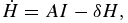
is positive. Notice that the first term is positive since σ > 1. A sufficient, not necessary condition for the Hamiltonian to be positive is thus that f(H) = θH α − (δ/A)H is positive at the time of death. The function f comes out of the origin, is concave and has another root at HR , as depicted in Figure A.1. The root is found at HR = (θA/δ)1/(1 − α). Since δ + ρβ > δ − δ(1 − α)β, we have
 \begin{equation}
\left({\theta A \over \delta } \right)^{1\over 1-\alpha } > \left({[1-(1-\alpha )\beta ]\theta A \over \delta +\rho \beta } \right)^{1\over 1-\alpha } { \ \Rightarrow \ }H_R > H^*.
\end{equation}
\begin{equation}
\left({\theta A \over \delta } \right)^{1\over 1-\alpha } > \left({[1-(1-\alpha )\beta ]\theta A \over \delta +\rho \beta } \right)^{1\over 1-\alpha } { \ \Rightarrow \ }H_R > H^*.
\end{equation}
This implies f(H*) > 0 and thus f(H(T)) > 0 for any H(T) < H*. A positive Hamiltonian at death means that the transversality condition is violated. It is not optimal to die.
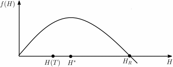
Figure A.1. The Curve f(H).


